Quantum phase transition with dissipative frustration

Abstract

We study the quantum phase transition of the one-dimensional phase model in the presence of dissipative frustration, provided by an interaction of the system with the environment through two non-commuting operators. Such a model can be realized in Josephson junction chains with shunt resistances and resistances between the chain and the ground. Using a self-consistent harmonic approximation, we determine the phase diagram at zero temperature which exhibits a quantum phase transition between an ordered phase, corresponding to the superconducting state, and a disordered phase, corresponding to the insulating state with localized superconducting charge. Interestingly, we find that the critical line separating the two phases has a non monotonic behavior as a function of the dissipative coupling strength. This result is a consequence of the frustration between (i) one dissipative coupling that quenches the quantum phase fluctuations favoring the ordered phase and (ii) one that quenches the quantum momentum (charge) fluctuations leading to a vanishing phase coherence. Moreover, within the self-consistent harmonic approximation, we analyze the dissipation induced crossover between a first and second order phase transition, showing that quantum frustration increases the range in which the phase transition is second order. The non monotonic behavior is reflected also in the purity of the system that quantifies the degree of correlation between the system and the environment, and in the logarithmic negativity as entanglement measure that encodes the internal quantum correlations in the chain.

I Introduction

Owing to the recent experimental progress, the investigation of the properties of artificial quantum many-body systems, or of synthetic quantum matter, has received great interest Buluta and Nori (2009); Cirac and Zoller (2012); Georgescu et al. (2014). Ultra-cold atoms in optical lattices Greiner et al. (2002); Bloch et al. (2012), trapped ions Barreiro et al. (2011); Blatt and Roos (2012) , exciton-polariton systems in semiconductor materials Kim and Yamamoto (2017), arrays of coupled QED cavities Leib and Hartmann (2010); Hartmann (2016), and superconducting circuits made by qubits and cavities Salathé et al. (2015); Barends et al. (2015) are the most remarkable experimental platforms. On one side, they are considered as quantum simulators to investigate the many-body problem in and out of thermal equilibrium. On the other side, they exhibit features that distinguish them from other strongly correlated systems in condensed matter. In these systems, the individual interacting units have to be considered as open or dissipative quantum systems as they are indeed macroscopic objects and can have relevant interactions with the environment. Typical examples are superconducting qubits in which energy relaxation and dephasing are unavoidable Makhlin et al. (2001); Zagoskin (2011); Li et al. (2014). Generally, quantum dissipative systems or systems with quantum reservoir engineering display a variety of interesting phenomena Biella et al. (2015); Zippilli et al. (2015); Hacohen-Gourgy et al. (2015); Labouvie et al. (2016); Wolff et al. (2016); Fitzpatrick et al. (2017); Fernández-Lorenzo and Porras (2017); Banchi et al. (2017); Raghunandan et al. (2018); Foss-Feig et al. (2017).

This intense research activity revived the study of dissipative phase transitions, originally initiated with Josephson junction arrays Fazio and van der Zant (2001). One-dimensional (1D) Josephson junction chains are an experimental realization of the 1D quantum phase model Wood and Stroud (1982); Bradley and Doniach (1984); Jacobs et al. (1984); Devillard (2011). They are formed by superconducting islands with a Josephson tunneling coupling between neighboring islands. Here, the quantum phase transition corresponds to a superconductor-insulator transition and occurs due to the competition of the Josephson coupling, which favors global phase coherence, and the electrostatic energy, which inhibits Cooper pair tunneling and favors the charge localization. The transition is activated by varying the ratio between the two energy scales, the Josephson (potential) energy $E_{J}$ and the characteristic charging (kinetic) energy $E_{C}$. This model - also known as rotor model - represents a paradigmatic statistical model to illustrate quantum phase transitions Sachdev (2007) and the mapping from a 1D quantum system to a 1D+1 classical one Sondhi et al. (1997). By mapping it into the XY model, theory predicts the phase transition in the 1D chain to be of Berezinsky-Kosterlitz-Thouless (BKT) type Bradley and Doniach (1984), with the superconducting phase having quasi ordering. In the BKT scenario, the fluctuations of the local phases diverge in the thermodynamical limit, while the fluctuations of the phase differences between neighbors are finite. In the rest of the paper we simply refer to the superconducting phase as ordered phase. Experiments on the scaling behavior of the resistance as a function of the temperature in finite size chains reported the predicted superconductor-insulator transition Chow et al. (1998); Kuo and Chen (2001). The quantum phase model also corresponds to the limit case of large average number of bosons per site in the lattice Bose-Hubbard model Fazio and van der Zant (2001); Fisher et al. (1989); Bruder et al. (1993). Applying a gate voltage (i.e., a chemical potential) to the chain, this system has a very rich phase diagram Fisher et al. (1989); Roddick and Stroud (1993); Bruder et al. (1993); van Otterlo et al. (1995); Freericks and Monien (1996); Odintsov (1996); Glazman and Larkin (1997); Sarkar (2007). In the limit of strong local Coulomb repulsion and when the gate voltage is set to a degeneracy point of two charges states of each island, the model maps onto the Heisenberg XXZ model Fazio and van der Zant (2001); Bruder et al. (1993). The disorder also leads to interesting effects in the phase diagram Bard et al. (2017), with glass phases that have been recently observed Cedergren et al. (2017). Similar complex phase diagrams have also been studied in superconducting Josephson circuits suitably wired up to implement the Frenkel-Kontorova model Yoshino et al. (2010), or in a chain formed by superinductors and small Josephson junctions Meier et al. (2015).

Dissipation breaks the equivalence between the classical and the quantum case as the dissipation strongly affects the equilibrium phase diagram in the quantum regime, whereas thermodynamics and dynamics are separated in classical systems. In terms of the mapping to the 1D+1 classical model, the effect of dissipation is to change the isotropic XY model to an anisotropic one leading to a dimensional crossover Panyukov and Zaikin (1987); Korshunov (1989); Bobbert et al. (1990, 1992). Being the local superconducting phase $\hat{\varphi}$ and the electrical charge on the islands $\hat{Q}$ canonically conjugated operators $[\hat{\varphi},\hat{Q}]=2ei$, the transition is affected by the interplay of these degrees of freedom. The phases of the superconducting condensate on the islands can be regarded as rotors where the Josephson coupling represents a ferromagnetic interaction, whereas the charging (kinetic) energy determines the strength of the quantum fluctuations. An increase of the ratio $E_{C}/E_{J}$ leads to the transition from an ordered, classical state to a quantum, disordered state of the phases.

Dissipative quantum phase transitions have been intensively studied in the 1D quantum phase model Chakravarty et al. (1986); Fisher (1987); Panyukov and Zaikin (1987); Chakravarty et al. (1988); Korshunov (1989); Zwerger (1989); Bobbert et al. (1990, 1992); Wagenblast et al. (1997); Refael et al. (2007) with the main result that dissipation suppresses quantum phase fluctuations thus favoring states with spontaneously broken symmetry and ordering of the phases. Experiments on linear Josephson junction chains with a tunable ratio of $E_{J}/E_{C}$ and different shunted resistance confirmed the predicted dissipative phase diagram Miyazaki et al. (2002).

 

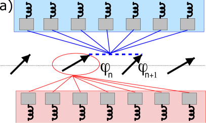
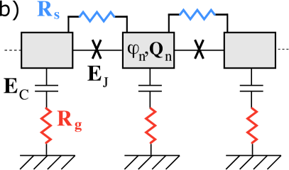
Figure 1: (a) Model for dissipative frustration in the 1D quantum phase model. The phase difference $\Delta\varphi_{n}$ for each link $n$ is coupled linearly to a bath (blue box) and the conjugated momentum of the phase is linearly coupled to a second, independent bath (red box). The external baths are represented as sets of independent harmonic oscillators. (b) 1D chain of superconducting islands with Josephson coupling of energy $E_{J}$ and charging energy $E_{C}$. The shunt resistance $R_{s}$ corresponds to a dissipative coupling for the difference of the superconducting phases $\varphi_{n}$, whereas the resistance to ground $R_{g}$ yields dissipative coupling in the charge $Q_{n}$.

A counter-example was given by a recent work in which the one-dimensional chain of Josephson junctions was assumed to be capacitively coupled to a proximate two-dimensional diffusive metal with a stabilization of the insulating ground state given by increasing the dissipation strength Lobos and Giamarchi (2011). From these results, one concludes that dissipation suppresses generally certain types of fluctuations associated to one degree of freedom, favoring one or other phases.

Remarkably, an open quantum system coupled to two independent environments via two canonically conjugate operators can yield interesting effects. This theoretical issues of “dissipative frustration” was analyzed for single open quantum system as a harmonic oscillator Kohler and Sols (2005, 2006); Cuccoli et al. (2010); Kohler and Sols (2013); Rastelli (2016), a single spin Castro Neto et al. (2003); Novais et al. (2005); Kohler et al. (2013); Bruognolo et al. (2014); Zhou et al. (2015), a Y shaped Josephson network Giuliano and Sodano (2008), as well as a lattice of interacting spins Lang and Büchler (2015). In other words, two environments couple to non commuting observables of a central system and are continuously monitoring the system leading to different and orthogonal conditioned states in presence of a single bath.

Figure 2: Sketch of the phase diagram of the 1D phase model with dissipative frustration. The critical line between the ordered phase and the disordered phase displays a non monotonic behavior.

In this work we study the effect of dissipative frustration on the quantum phase transition for the one-dimensional phase model. The dissipative coupling through the conjugate operators is realized by assuming that each local phase difference is coupled to a local bath (or conventional phase dissipation) and each local momentum coupled to another local bath (unconventional or charge dissipation), see Fig. 1(a). These two kinds of dissipative interaction compete since, when they are considered separately, they suppress different quantum fluctuations, viz. phase or charge, whose product is bound by the uncertainty principle.
We show that this model can be realized by a chain of Josephson junctions with equal shunted resistance $R_{s}$ between neighboring islands - to encode the phase dissipation - and resistances $R_{g}$ between each superconducting island and the ground - to encode the charge dissipation - as shown in Fig. 1(b).
We use a variational approach, the self-consistent harmonic approximation (SCHA) Chakravarty et al. (1986, 1988); Kugler (1969); Gillis and Koehler (1972); Moleko and Glyde (1983); Kampf and Schön (1987); Samathiyakanit and Glyde (1973); Rastelli and Ciuchi (2005); Rastelli and Cappelluti (2011), to treat the non-linear Josephson coupling between the phases. The SCHA allows to take into account the anharmonic effects for large quantum phase fluctuations eventually leading to the transition. Within the SCHA, we construct a phase diagram for the ordered-disordered phase transition (superconductor-insulator) in terms of the dissipative coupling and the ratio between the two energy scales $E_{J}/E_{C}$ that measures, qualitatively speaking, the amount of the intrinsic quantum phase fluctuations in the ordered phase of the isolated chain. For a given ratio between the two dissipative coupling strengths, our main result is that the critical line has a non monotic behavior for increasing total dissipation of the system, see Fig. 2. On the basis of the SCHA, we discuss the order of the phase transition and the crossover from a first order to second order phase transition.
A non-monotonic dependence of the critical value was previously reported in a dissipative 2D Josephson array in different geometries due to non-local dissipation in Ref. Polak and Kopeć (2007) or due to an applied magnetic field in Ref. Polak and Kopeć (2005). However, the critical line as a function of the dissipative strength was monotonic in agreement with the expected behavior in presence of phase dissipation.
Since the dissipative phase transition is triggered by quantum fluctuations at zero temperature, which are strongly affected by the interaction of the system with the environments, we study the purity of the system that quantifies the correlation between the system and the environment. The purity shows a non monotonicity close to the critical point at the phase transition, pointing out that the correlation with the environment plays an important role. We also calculate the logarithmic negativity as entanglement measure that encodes the internal quantum (non classical) correlations in the system and show that this quantity can also have a non monotonic behavior approaching the phase transition. From these results, we can conclude that the dissipative phase transition has a spurious nature in which internal (quantum) correlations as well as extrinsic (statistical) correlations have similar weight.

This paper is structured as follows. In Sec. II we introduce the quantum phase model with dissipative frustration in terms of the path integral formalism Feynman et al. (2010); Kleinert (2009); Weiss (2012), namely we introduce the effective action in the imaginary time representation. We also present the self-consistent harmonic approximation (SCHA) and the results of the phase difference fluctuations between neighboring phases, a quantity that plays a central role in the SCHA. In Sec. III we discuss the results for the phase diagram in presence of dissipative frustration whose main effect is sketched in the Fig. 2. In Sec. IV, we classify the order of the phase transition within the SCHA by analyzing the behavior of the variational expansion for the free energy that represents an upper bound estimation of the exact free energy. In Sec. V, we present the results for the purity and the logarithmic negativity. Finally, in Sec. VI we summarize our work and draw our conclusions. Appendixes A and B contain the derivation of the path integral action related to the unconventional (charge) dissipation. In Appendix C we recall the method to calculate the logarithmic negativity using the correlation matrix. In Appendix D we report further results for the entanglement measure that confirm the behavior discussed in the main text for different configurations of the two subsystems in which the chain is bipartite.

II Model and Approximations

In this section we introduce the dissipative phase model and the corresponding effective action. We then present the SCHA and report the main steps of our calculations in obtaining the analytic expressions of the quantum phase fluctuations.

II.1 Hamiltonian

We consider a 1D chain of $N$ rotors of radius $R$ whose dynamics is described by the local phase operators $\hat{x}_{n}=R\hat{\varphi}_{n}$ and momenta $\hat{p}_{n}=(\hbar/iR)\partial/\partial\hat{\varphi}_{n}$, with the commutation relation $[\hat{x}_{n},\hat{p}_{m}]=i\hbar\delta_{nm}$. The phases interact via a nearest-neighbor pairwise potential $U(\Delta\hat{\varphi}_{n})=-V\cos(\Delta\hat{\varphi}_{n})$, where $\Delta\hat{\varphi}_{n}=\hat{\varphi}_{n+1}-\hat{\varphi}_{n}$. We assume periodic boundary conditions $\hat{\varphi}_{N}\equiv\hat{\varphi}_{0}$. The Hamiltonian of the considered system reads

$$\hat{H}_{S}=\sum_{n=0}^{N-1}\left[-\frac{K}{2}\left(\partial^{2}/\partial\hat{\varphi}^{2}\right)-V\cos(\Delta\hat{\varphi}_{n})\right]\,,$$ (1)

where $K=\hbar^{2}/(mR^{2})$ is the energy scale associated to the kinetic energy of the rotors.

This is the same Hamiltonian as for a chain of superconducting islands with a Josephson coupling $E_{J}$ between nearest neighbors and a capacitance to the ground $C_{0}$ with charging energy $E_{C}=4e^{2}/C_{0}$. In the representation of the charge operator $\hat{N}_{n}=\sum_{N_{n}}N_{n}\left|N_{n}\right>\left<N_{n}\right|$ with $\left|N_{n}\right>$ the number states and $N_{n}$ corresponding to the Cooper pair number in each superconducting island, the system Hamiltonian takes the form

$$\hat{H}_{S}=\frac{E_{C}}{2}\sum_{n=0}^{N-1}{\left(\hat{N}_{n}-N_{0}^{\phantom{g}}\right)}^{2}-E_{J}\left(\hat{T}_{n,n+1}^{\phantom{g}}+\hat{T}_{n,n+1}^{\dagger}\right)\,,$$ (2)

with the quantum tunneling operator describing the coherent hopping of Cooper pairs given by Zagoskin (2011); Tinkham (1996)

$$\hat{T}_{a,b}=\left|N_{a},N_{b}+1\right>\left<N_{a}+1,N_{b}\right|\,.$$ (3)

Introducing the phase operator $\hat{\varphi}_{n}$ conjugate to $\hat{N}_{n}$, we have the Hamiltonian Zagoskin (2011); Tinkham (1996)

$$\hat{H}_{S}=\sum_{n=0}^{N-1}\left[-\frac{E_{C}}{2}\left(\partial^{2}/\partial\hat{\varphi}^{2}\right)-E_{J}\cos(\Delta\hat{\varphi}_{n})\right]\,.$$ (4)

The Hamiltonian (4) is based on the assumption that the quasiparticle excitations (above the gap) can be neglected, see Ref. Fazio and van der Zant (2001). At zero temperature, the behavior of the quantum phase model is fully described by the dimensionless ratio $g=\sqrt{V/K}=\sqrt{E_{J}/E_{C}}$. In the limit of small phase difference fluctuations for $E_{J}\gg E_{C}$ ($g\gg 1$), one can expand the potential in Eq. (4) to harmonic order and obtains that the average quantum phase difference fluctuations are controlled by the inverse of this ratio, viz. ${\left<\Delta\hat{\varphi}^{2}\right>}_{har}=\sqrt{2}/g$.

II.2 Effective action and dissipation

Dissipation arises when we consider the interaction of the chain with the environment. Then, to discuss the equilibrium properties of an open quantum system, the imaginary time path integral formalism allows to integrate out the degrees of freedom associated to the environment and focus only on the partition function associated to the degrees of freedom of the system, viz. the phases. In our case, the effective partition function $\mathcal{Z}_{\rm eff}$ describing the phase model reads

$$\mathcal{Z}_{\rm eff}=\prod_{n=0}^{N-1}\oint_{c}\mathcal{D}[\varphi_{n}(\tau)]\,\,e^{-\mathcal{S}[\{\varphi_{n}(\tau)\}]/\hbar}\,\,,$$ (5)

where the symbol $\oint_{c}$ refers to the path integral over imaginary time for the interval $0<\tau<\beta$ , with $\beta=\hbar/(k_{B}T)$ and to periodic boundary conditions for the phase variable $\varphi$, i.e. $\varphi(0)=\varphi(\beta)$ foo Apenko (1989). The effective Euclidean action for the system is given by

$$\mathcal{S}=\mathcal{S}_{diss}-\int_{0}^{\beta}\!\!\!\!\!d\tau E_{J}\cos\left(\Delta\varphi_{n}(\tau)\right)\,$$ (6)

where the quadratic action is

$$\mathcal{S}_{diss}= -\sum_{n=0}^{N-1}\frac{1}{2}\int_{0}^{\beta}\!\!\!\!\int_{0}^{\beta}\!\!d\tau d\tau^{\prime}\,F(\!\tau\!-\!\tau^{\prime})\,{\left|\Delta\varphi_{n}(\tau)-\Delta\varphi_{n}(\tau^{\prime})\right|}^{2}$$

$$+\sum_{n=0}^{N-1}\frac{1}{2}\int_{0}^{\beta}\!\!\!\!\int_{0}^{\beta}\!\!d\tau d\tau^{\prime}\,\widetilde{F}(\!\tau\!-\!\tau^{\prime})\,\dot{\varphi}_{n}(\tau)\,\dot{\varphi}_{n}(\tau^{\prime})\,,$$ (7)

with $\dot{\varphi}=d\varphi/d\tau$. Note that the action (II.2) is locally invariant under a variation of $2\pi$ of the phase.

The first term of Eq. (II.2) corresponds to the conventional or phase dissipation associated to the shunt ohmic resistance between two superconducting islands Fazio and van der Zant (2001); Chakravarty et al. (1986, 1988); Zwerger (1989); Bobbert et al. (1990, 1992). Using the Fourier transform in the imaginary time for the $\beta-$periodic function $x(\tau)=\sum_{\ell}x_{\ell}e^{i\omega_{\ell}\tau}$ with the Matsubara frequencies $\omega_{\ell}=(2\pi/\beta)\ell$ and $\ell$ integer, the component of the ohmic kernel $F(\tau)$ is Chakravarty et al. (1986, 1988); Bobbert et al. (1990, 1992); Fazio and van der Zant (2001); Weiss (2012):

$$F_{\ell}=\frac{\hbar}{4\pi\beta}\left(\frac{R_{q}}{R_{s}}\right)\left|\omega_{\ell}\right|f_{c}(\omega_{\ell})\,,$$ (8)

with $F_{\ell=0}=0$ and the Drude cutoff function at large frequency $\omega_{c}$ of the form $f_{c}(\omega)=0$ for $\omega/\omega_{c}\rightarrow\infty$. The parameter that quantifies the dissipative coupling strength is associated to the ratio between the quantum resistance $R_{q}=h/(4e^{2})$ and the shunt resistance $R_{s}$

$$\alpha=R_{q}/R_{s}=\gamma(h/E_{C})\quad\mbox{with}\,\,\,\gamma=1/(R_{s}C_{0})\,,$$ (9)

whereas the rate $\gamma$ corresponds to the friction coefficient. In the limit $R_{s}/R_{q}\rightarrow\infty$, the current flowing through the shunt resistances vanishes and the 1DJJ chain is not affected by the conventional dissipation.

The second term of Eq. (II.2) includes the kinetic energy and the unconventional or charge dissipation, with the Matsubara components given by the expression

$$\widetilde{F}_{\ell}=\frac{\hbar^{2}}{\beta E_{C}}\left(1-\frac{R_{g}C_{0}\left|\omega_{\ell}\right|f_{c}(\omega_{\ell})}{1+R_{g}C_{0}\left|\omega_{\ell}\right|f_{c}(\omega_{\ell})}\right)\,,$$ (10)

whose explicit derivation is provided in the Appendices A and B. Here we simply observe that this expression can be derived by duality between the two conjugate quadratures of a harmonic oscillator coupled separately to two baths Kohler and Sols (2006); Rastelli (2016). In other words, it is possible to show that unconventional dissipation as given by Eq. (10) yields a quenching of the momentum quantum fluctuations which is exactly equivalent to the quenching of the phase quantum fluctuation for an oscillator affected by ohmic damping given by Eq. (8). In the quantum phase model, the parameter that quantifies the strength of the charge dissipative coupling is related to the characteristic time scale of the impedance due to the resistance to the ground $R_{g}$ in series with the capacitance $C_{0}$, see Fig. 1 (b). In contrast to the phase dissipation, the dissipative coupling vanishes in the limit $R_{g}\rightarrow 0$. It is useful to introduce the parameter

$$\widetilde{\alpha}=R_{g}/R_{q}=\tau_{g}(E_{C}/h)\quad\mbox{with}\,\,\,\tau_{g}=R_{g}C_{0}\,$$ (11)

playing the role of the dimensionless coupling constant of the unconventional dissipation.
To be specific, we assume as a cutoff frequency $f_{c}(\omega_{\ell})=1/\left(1+\left|\omega_{\ell}\right|/\omega_{c}\right)$ in the following. For $R_{g}=0$, the model of the action (6) corresponds to the dissipative quantum rotor model discussed extensively in the literature Fazio and van der Zant (2001); Panyukov and Zaikin (1987); Korshunov (1989); Bobbert et al. (1990, 1992); Chakravarty et al. (1986); Fisher (1987); Chakravarty et al. (1988); Zwerger (1989); Wagenblast et al. (1997); Refael et al. (2007). Note that we focus on the case of homogeneous dissipation assuming the two kernel functions $F(\!\tau\!)$ and $\widetilde{F}(\!\tau\!)$ to be independent of the position on the lattice (index $n$).

II.3 The self-consistent harmonic approximation SCHA

In the limit in which the average phase difference fluctuations are small $\sqrt{\left<\Delta\varphi^{2}\right>}\ll\pi$, we can use the harmonic approximation and expand the potential to obtain

$$\mathcal{S}_{\rm harm.}=\mathcal{S}_{diss}+\sum_{n=0}^{N-1}\int_{0}^{\beta}\!\!\!\!d\tau\,E_{J}\left[-1+\frac{1}{2}\Delta\varphi_{n}^{2}(\tau)\right]\,.$$ (12)

If the fluctuations are strongly localized, paths of large fluctuations $\varphi(\tau)\sim\pi$ are extremely unlikely to occur.

Beyond the harmonic approximation valid at $\sqrt{\left<\Delta\varphi^{2}\right>}\ll\pi$, the model of Eq. (6) can not be solved exactly in general due to the presence of the interaction potential and we have to resort to an approximated scheme. For larger values of the phase fluctuations, further anharmonic terms of the pairwise potential, have to be taken into account. To treat this regime, we employ the self-consistent harmonic approximation (SCHA) Chakravarty et al. (1986, 1988); Kugler (1969); Gillis and Koehler (1972); Moleko and Glyde (1983); Kampf and Schön (1987); Samathiyakanit and Glyde (1973); Rastelli and Ciuchi (2005); Rastelli and Cappelluti (2011). Within this approach, a quadratic trial action $\mathcal{S}_{tr}$ is introduced as

$$\mathcal{S}_{tr}=\mathcal{S}_{diss}-\beta NE_{J}+\sum_{n=0}^{N-1}\int_{0}^{\beta}\!\!\!\!\!d\tau\,\frac{1}{2}V_{tr}\,\Delta\varphi_{n}^{2}(\tau)\,$$ (13)

which is formally equivalent to the harmonic expansion of Eq. (12). However, one assumes $V_{tr}$ as a free variational parameter, different from the bare energy constant of the potential $V_{tr}\neq E_{J}$. Similarly to the harmonic expansion, the partition function associated to the action (13) can be computed by $\mathcal{Z}_{tr}=\prod_{n=0}^{N-1}\oint\mathcal{D}[\varphi_{n}(\tau)]\,\,\exp({-\mathcal{S}_{tr}/\hbar})$, together with the Helmoltz free energy $\mathcal{F}_{tr}=-(\hbar/\beta)\ln[\mathcal{Z}_{tr}]$. Using the Bogoliubov inequality, an upper bound for the exact free energy $\mathcal{F}_{\rm eff}=-(\hbar/\beta)\ln[\mathcal{Z}_{\rm eff}]$

$$\mathcal{F}_{\rm eff}\,\leq\mathcal{F}_{v},\;\;\;\;\;\;\; \mathcal{F}_{v}=\mathcal{F}_{tr}+(\hbar/\beta){\langle\mathcal{S}-\mathcal{S}_{tr}\rangle}_{tr}\,,$$ (14)

where the average ${\langle\mathcal{S}-\mathcal{S}_{tr}\rangle}_{tr}$ is performed on the variational action $\mathcal{S}_{tr}$. The minimum of the r.h.s of Eq. (14) is determined by taking the derivative respect to the variational parameter $V_{tr}$ and setting it to zero. This leads to the following self-consistent equation for the variational parameter

$$V_{sc}=E_{J}\,e^{-\frac{1}{2}{\langle\Delta\varphi^{2}\rangle}_{sc}}\,,$$ (15)

containing the fluctuations of the phase difference ${\langle\Delta\varphi^{2}\rangle}_{sc}$ calculated on the variational action (13) for $V_{tr}\rightarrow V_{sc}$, i.e. the self-consistent parameter, representing the effective spin-wave stiffness constant Chakravarty et al. (1986). This way, the SCHA captures the anharmonic behavior of the phase fluctuations by an effective harmonic potential $V_{sc}$ which approximates the actual anharmonic fluctuations.

This one-component theory of the phase transition provides a (qualitative) phase diagram in the following way: By varying one of the parameters $g$, $\alpha$ or $\tilde{\alpha}$, one can determine the critical value above which there is no solution of Eq. (15). This solution corresponds to a spinodal point which, in the SCHA, is associated to the transition between the ordered phase, characterized by (an)harmonic fluctuations of the phases, and the disordered phase without any long-range correlations. An alternative criterion to derive the critical line consists in comparing the upper bound of the exact free energy evaluated at the self-consistent solution $\mathcal{F}_{\rm eff}(V_{tr}=V_{sc})$ with the value for vanishing stiffness constant $\mathcal{F}_{\rm eff}(V_{tr}=0)$: then the critical point corresponding to the situation in which $\mathcal{F}_{\rm eff}(V_{sc})\geq\mathcal{F}_{\rm eff}(0)$, identifies the transition to the disordered phase. The latter criterion allows to distinguish between a first and second order phase transition.

In the following , we discuss both criteria to obtain the phase diagram for the 1D dissipative system of phases with conventional (or phase) dissipation and unconventional (or charge) dissipation.

II.4 Calculation of the quantum phase fluctuations

In this subsection we discuss the analytic expression for the quantum phase difference fluctuations, in the limit of zero temperature $\beta\rightarrow\infty$ $(T\rightarrow 0)$, calculated on the quadratic trial action (13). The Gaussian trial action can be decomposed in terms of non interacting quadratic modes which are defined by the relation $\varphi_{n}=(1/\sqrt{N})\sum_{k=0}^{N-1}e^{-i2\pi kn/N}\varphi_{k}$ . Then the average phase fluctuations are expressed as

$${\langle\Delta\varphi^{2}\rangle}_{sc} =\frac{4}{N}\sum_{k=1}^{N-1}\sin^{2}\left(\frac{\pi k}{N}\right){\langle{\left|\varphi_{k}\right|}^{2}\rangle}_{\!sc}\,$$ (16)

in which each term corresponds to the fluctuations of a harmonic mode. To calculate ${\langle{\left|\varphi_{k}\right|}^{2}\rangle}_{\!sc}$, we express $\{\varphi_{n}\}$ as functions of $\{\varphi_{k}\}$ in the Gaussian action (13), and obtain the Lagrangian of $N$ independent harmonic oscillators, each of them affected by conventional and unconventional dissipation.

By proceeding in a similar way as in Ref. Chakravarty et al. (1988), we arrive at the expression:

$${\langle{\left|\varphi_{k}\right|}^{2}\rangle}_{\!sc}\!\!=\!\!\sum_{l=-\infty}^{+\infty}\frac{E_{C}/(\hbar\beta)}{\left(\omega_{k}^{(sc)}\right)^{2}+\frac{4\sin^{2}\left(\frac{\pi k}{N}\right)|\omega_{l}|\alpha E_{C}/h}{1+\frac{|\omega_{l}|}{\omega_{c}}}+\frac{\omega_{l}^{2}}{1+\frac{\tau_{g}|\omega_{l}|}{\left(1+\frac{|\omega_{l}|}{\omega_{c}}\right)}}}\,,$$ (17)

where the eigenfrequencies

$$\omega_{k}^{(sc)} =2\,\frac{\sqrt{E_{C}V_{sc}}}{\hbar}\,\sin\left(\pi k/2N\right)\,.$$ (18)

corresponding to the frequency of the normal modes of the Josephson chain. Since, we are interested in the quantum regime, we take the zero temperature limit $\beta\rightarrow\infty$, and the sum over Matsubara frequencies transforms into an integral that can be calculated analytically. Thus we obtain the expression

$${\langle{\left|\varphi_{k}\right|}^{2}\rangle}_{\!sc}=\frac{\phi_{a}+\phi_{b}}{\pi g^{2}}+2\widetilde{\alpha}\frac{\ln\left[\omega_{c}/\omega_{k}^{(sc)}\right]}{1+\sigma^{2}_{k}}$$ (19)

where we introduced $\sigma_{k}^{2}=4\sin^{2}(\pi k/N)\alpha\tilde{\alpha}$, the two phases

$$\phi_{a} = \frac{2\pi g^{2}\tilde{\alpha}}{1+\sigma_{k}^{2}}\left[\ln(1+\sigma_{k}^{2})+\sigma_{k}\arctan(\sigma_{k})\right]$$ (20)

$$\phi_{b} = \frac{1}{1+\sigma_{k}^{2}}\left(\!\!\frac{E_{J}}{\mbox{}\,\,\hbar\omega_{k}^{(sc)}}+2\pi g^{2}\tilde{\alpha}\,\Gamma_{-}^{(sc)}\!\!\right)\mathcal{\mathbb{F}}\!\!\left[\Gamma_{-}^{(sc)}\!\!,\Gamma_{+}^{(sc)}\right]\,.$$ (21)

and the function

$$\mathcal{\mathbb{F}}[x,y]=\begin{cases}\frac{1}{\sqrt{1-x^{2}}}\text{arctan}\left(\frac{\sqrt{1-x^{2}}}{y}\right)&,\text{for}\,x<1\\ \frac{1}{\sqrt{x^{2}-1}}\text{arctanh}\left(\frac{\sqrt{x^{2}-1}}{y}\right)&,\text{for}\,x>1\end{cases}\,$$ (22)

with the parameter $\Gamma_{\pm}^{(sc)}=\sin^{2}\left(\pi k/N\right)\alpha E_{C}/(\pi\hbar\omega_{k}^{(sc)})\pm\pi(\hbar\omega_{k}^{(sc)}/E_{J})g^{2}\tilde{\alpha}$. We recover the previous result Rastelli (2016) for $V_{sc}=E_{J}$. The analytical expression (19) for each harmonic mode was obtained in presence of a high frequency cutoff $\omega_{c}\gg\omega_{k}^{(sc)},\gamma,1/\tau_{g}$. Note the logarithmic dependence on $\omega_{c}$ in Eq. (19), characteristic for the ohmic dissipation with a Drude cutoff Weiss (2012).

Once the fluctuations ${\langle\Delta\varphi^{2}\rangle}_{sc}$ are expressed in terms of both coupling constants $\alpha$, $\widetilde{\alpha}$ and $g$, we use Eqs. (16) and (19) to solve the self-consistent equation (15) numerically. As explained above, within the SCHA framework the existence of a solution of (15) corresponds to the ordered state of the rotors, whereas one associates its disappearance to a phase transition of the system towards a disordered state. The SCHA approach can only be justified, a priori, for fluctuations $\sqrt{\langle\Delta\varphi^{2}\rangle_{sc}}\lesssim\pi$. Nonetheless, we use this approximation to gain a first qualitative understanding of the influence of the conjugate baths on the quantum phase transition.

II.5 Absence of dissipation ($\alpha=\tilde{\alpha}=0$)

As discussed in the introduction, in absence of dissipation, decreasing $g$ below a critical value leads to a phase transition. Before presenting the numerical results including dissipation, we illustrate the prediction of the SCHA equation for this case. For $\alpha=\tilde{\alpha}=0$ and in the limit $N\gg 1$, the self-consistent Eq. (15) simplifies to

$$V_{sc}/E_{J}=e^{-\frac{1}{\pi g}\sqrt{E_{J}/V_{sc}}}\,.$$ (23)

We denote the maximum value corresponding to the critical solution of Eq. (23) by $g_{s}^{(0)}$. In correspondence of this point, the l.h.s. and r.h.s. of (23) have the same derivative with respect to the variable $x=V_{sc}/E_{J}$. Using the latter condition together with Eq. (23), we find $\sqrt{V_{sc}/E_{J}}=1/(2\pi g_{s}^{(0)})$ that yields $V_{sc}/E_{J}=1/e^{2}$ and corresponds to a critical value $g_{s}^{(0)}=e/(2\pi)\approx 0.43$ .

III Results: solution of the self-consistent equation

We here present the results for the solutions of the self-consistent equation (15). We consider a high frequency cutoff $\hbar\omega_{c}=100E_{C}$ corresponding to the regime $\omega_{c}\gg\omega_{k},\gamma,1/\tau_{g}$, and $N=150$ for which the phase difference fluctuations are converged and close to the thermodynamical limit, i.e. further doubling of $N$ affects the results by less than $0.07$ percent. In this section, we set the notation $\delta\varphi_{sc}=\sqrt{\langle\Delta\hat{\varphi}_{n}^{2}\rangle_{sc}}$ for the quantum phase difference fluctuations calculated with the self consistent parameter $V_{sc}$.

We first discuss the conventional dissipation $\alpha>0$ and $\widetilde{\alpha}=0$ for which we recover previous results obtained with the SCHA Chakravarty et al. (1986, 1988). In Fig. 3(a) we show $\delta\varphi$ for different values of $\alpha$, by varying the system parameter $g$. For reference, we also plot the dissipationless case $\alpha=0$ (black solid line). The endpoint of each line corresponds to the critical value $g_{s}(\alpha)$, where the SCHA solution vanishes.

For a fixed value of $g$, the phase fluctuations decrease with increasing damping. As a consequence, the critical value $g_{s}$, determined by the critical solution of the self-consistent equation, decreases. The corresponding phase diagram is shown in Fig. 3(c), reporting the critical values $g_{s}$. From this result, one can conclude that the dissipation stabilizes the ordered phase of the system. Indeed, a more refined treatment beyond the SCHA yields the same qualitative behavior of the critical line, namely the negative slope of $\alpha$ vs $g_{s}$ with a shift towards smaller critical values Bobbert et al. (1990); Panyukov and Zaikin (1987); Korshunov (1989).

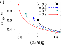
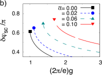
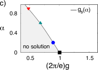
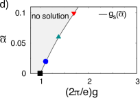
Figure 3: $\delta\varphi_{sc}$ as a function of the parameter $g$, for different values of the conventional damping $\alpha$ in (a), and of the unconventional damping $\widetilde{\alpha}$ in (b). The endpoints determine the critical values of $g_{s}(\alpha)$ and $g_{s}(\widetilde{\alpha})$ below which there is no solution of the self-consistent equation. In (c) and (d) the sets of the critical points $g_{s}(\alpha)$ and $g_{s}(\widetilde{\alpha})$ are shown for the different damping coefficients. The gray area denotes where the self-consistent equation has no solution.

We now consider the opposite limit of purely unconventional dissipation affecting the system, i.e. $\widetilde{\alpha}>0$ and $\alpha=0$. The behavior of the fluctuations as a function of $g$ and for different values of $\widetilde{\alpha}$ is shown in Fig. 3(b). Again, the black solid line corresponds to the dissipationless case $\widetilde{\alpha}=0$. Compared to the previous results, the system displays now an opposite behavior: for a fixed value of $g$, the phase fluctuations increase with increasing damping. This can be explained by the Heisenberg uncertainty relation: the unconventional dissipation quenches the zero-point fluctuations of the momentum (charge) $\delta p$ leading to an increase of the phase and phase-difference fluctuations $\delta\varphi\sim\hbar/\delta p$. As shown in Fig. 3(d), the unconventional dissipation leads to an increasing critical value $g_{s}(\widetilde{\alpha})$. A qualitatively similar result was obtained for the phase diagram of the superconductor/insulator transition occurring in a chain of Josephson junctions that was capacitively coupled to a metallic conducting film in the diffusive regime Lobos and Giamarchi (2011).

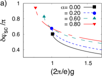
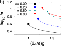
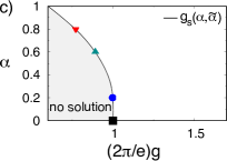
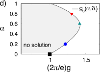
Figure 4: $\delta\varphi_{sc}$ as a function of the parameter $g$, for different values of the conventional damping $\alpha$ at a given ratio of $\widetilde{\alpha}/\alpha=0.1$ in (a), and $\widetilde{\alpha}/\alpha=0.3$ in (b). The endpoints determine the critical value of $g_{s}(\alpha,\widetilde{\alpha})$, below which there is no solution of the self-consistent equation. These are reported in (c) for $\widetilde{\alpha}/\alpha=0.1$, and in (d) for $\widetilde{\alpha}/\alpha=0.3$. The gray area denotes where the self-consistent equation has no solution.

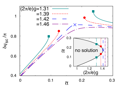
Figure 5: $\delta\varphi_{sc}$ as a function of the parameter $\widetilde{\alpha}$ (with the ratio $\widetilde{\alpha}/\alpha=0.3$), for different values of $g$. The end points determine the critical value(s), above which there is no solution of the self-consistent equation (see shaded area in the inset displaying the phase diagram in $\widetilde{\alpha}$ and $g$).

We now analyze the general case when both types of dissipation are present: $\alpha>0$ and $\widetilde{\alpha}>0$.

Since conventional (or phase) dissipation quenches the phase fluctuations whereas unconventional (or momentum) dissipation yields a quenching of the momentum fluctuations, we expect a competition of the two types of dissipative interactions as they affect two canonically conjugate operators. In Figs. 4(a) and (c) we show the results for a given ratio $\widetilde{\alpha}/\alpha=0.1$, for which we obtain a qualitatively similar behavior to the case of $\widetilde{\alpha}=0$. A different behavior occurs in the regime when momentum dissipation has a stronger influence. As an example of this regime, we show in Figs. 4(b) and 4(d) the results for the ratio $\widetilde{\alpha}/\alpha=0.3$. In this case, the trend appears to be inverted: increasing the overall dissipative coupling strength, the values $g_{s}(\alpha,\widetilde{\alpha})$ exhibit a non monotonic behavior. Starting from a small value of the dissipation ($\alpha=0.2$ or $\widetilde{\alpha}=0.06$), the critical value increases, as in the case of purely unconventional dissipation. However, for larger values of dissipation ($\alpha>0.6$ or $\widetilde{\alpha}>0.18$) $g_{s}(\alpha,\widetilde{\alpha})$ decreases, as in the case of a purely conventional dissipation.

In order to gain a better understanding of this regime, we also report the phase fluctuations as a function on the damping coefficient at a fixed ratio $\widetilde{\alpha}/\alpha$, and for different values of $g$ (see Fig. 5). For large values $(2\pi/e)g\geq 1.42$, we always obtain a solution for the self-consistent equation for all values of the damping coefficient. As long as $(2\pi/e)g\leq 1.42$, there is a solution for both small and large values of the dissipative strength interaction, whereas there is a region of no solution at intermediate values. This result stems from the behavior of the quantum fluctuations for the position or momentum of a harmonic oscillator with two non commuting dissipative interactions. In this case, the fluctuations show a non monotonic behavior as a function of the dissipative coupling strength Rastelli (2016). For instance, at $(2\pi/e)g=1.42$ , in Fig. 5, it is possible to observe a weak non monotonic behavior. However, in contrast to a pure harmonic oscillator for which strong fluctuations are always allowed at any scale, the solution for the self-consistent equation vanishes at large phase fluctuations and this produces a cut of the lines for values $(2\pi/e)g<1.42$, shown in Fig. 5.

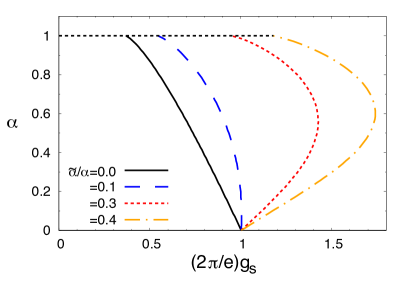
Figure 6: Critical line $g_{s}(\alpha,\widetilde{\alpha})$ with dissipative frustration. Right to the transition line is the ordered phase, on the left the rotors are randomly orientated (see Fig. 2). By increasing the ratio $\widetilde{\alpha}/\alpha$ the non monotonic behavior is more pronounced.

Finally, we analyze the evolution of the phase diagram between the two regimes of Fig. 4(c) and (d), and plot the critical line $g_{s}(\alpha,\widetilde{\alpha})$ and for different ratios $\widetilde{\alpha}/\alpha$ in Fig. 6. The region to the right of the transition line presents a solution of the self-consistent equation and is associated to the phase with phase ordering, whereas in the region to the left there is no self consistent solution. Further, as previously reported (see Ref. Chakravarty et al. (1988) for example), above the critical damping $\alpha_{C}=1$ the system is always in the ordered phase.

As discussed above, at small dissipative coupling strengths we observe an evolution from the regime of negative to positive slope of the critical line. Moreover, the critical line exhibits a change in the global behavior. In the regime $\widetilde{\alpha}/\alpha<\xi$, with the critical threshold $\xi\approx 0.1$, the critical value $g_{s}$ decreases with the dissipative coupling. In the opposite regime $\widetilde{\alpha}/\alpha>\xi$, the critical value $g_{s}$ first increases with the dissipative coupling and then decreases again at larger damping. Such non monotonic behavior is more pronounced for larger values of the ratio $\widetilde{\alpha}/\alpha$. The phase diagram reported in Fig. 6 implies the interesting possibility that, for a given ratio of the parameter $g$, the system exhibits two phase transitions by increasing the dissipation: the first one from the ordered phase to the disordered phase and then, by further increasing the damping, one drives the system back to the ordered phase, see Fig. 5.

IV ORDER of the PHASE TRANSITION

In this section we consider the phase diagram of the system by using a criterion of Eq. (14) based on the upper bound $\mathcal{F}_{v}(V_{tr}=V_{sc})$ of the free energy $\mathcal{F}_{\rm eff}$, where $V_{sc}$ is the self-consistent solution of Eq. (23). When $\mathcal{F}_{v}(V_{sc})\geq\mathcal{F}_{v}(0)$, the real local minimum in the SCHA corresponds to the solution $V_{tr}=0$ which represents the real upper bound estimation of the exact free energy. Within the SCHA, this point corresponds to the phase transition in which the spin-wave stiffness vanishes and the system is in the disordered state.

An example of the behavior of $\mathcal{F}_{v}(V_{tr})$ is reported in Fig. 7, showing the free energy for different values $\alpha$ with frustrated dissipation. In this figure, the circle corresponds to the spinodal point of the self-consistent equation, while the black dots to the condition $\mathcal{F}_{v}(V_{sc})=\mathcal{F}_{v}(0)$. The latter condition occurs at a value of $g_{c}$ which is generally larger than the $g_{s}$ found by the self-consistent Eq. (23). Hence, the phase transition shifts to larger values of $g$. This jump, from a finite value of $V_{sc}$ to zero, corresponds to a first order phase transition.

However, by increasing the coupling strength $\alpha$ we see that the difference between the spinodal point and the global minimum disappears. In particular, for values $\alpha>1$ the system is always in the ordered state and the point at $V_{tr}=0$ is a maximum for all values of $g>0$. At the point $\alpha_{C}=1$ the transition turns to be of second order.

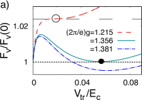
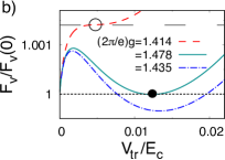
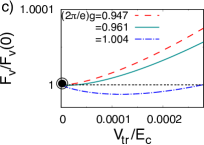
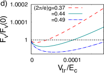
Figure 7: Upper bound $\mathcal{F}_{v}(V_{tr})$ for free energy in Eq. (14) as a function of $V_{tr}$ in presence of dissipative frustration, for the ratio $\widetilde{\alpha}/\alpha=0.3$ and a) $\alpha=0.2$, b) $\alpha=0.6$, c) $\alpha=1.0$ and d) $\alpha=1.5$. The empty circles correspond to the spinodal point, i.e. the disappearance of the finite solution $V_{sc}$ in the self consistent equation (23). The solid dots correspond to the phase transition according to the criterion $\mathcal{F}_{v}(V_{sc})=\mathcal{F}_{v}(0)$.

To summarize we can identify three regimes. In the low damping regime we have a first order phase transition, see Fig. 7(a,b). Increasing the damping the jump in the parameter gets smaller and we call the transition ”weakly” first order, Fig. 7(c). Further increasing the damping, $V_{sc}$ tends continuously to zero and we have a second order phase transition, Fig. 7(d). We illustrate those three regimes by plotting the phase diagrams originating from the self-consistent equation discussed in the previous section with the one obtained from the free energy minimum. Fig. 8 shows the phase diagrams of the two different criteria (dashed black line for the spinodal points, blue solid line for the free energy approach).

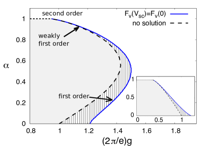
Figure 8: Quantum phase diagram with dissipative frustration for the ratio $\widetilde{\alpha}/\alpha=0.3$. The solid line and the dashed line correspond, respectively, to the phase transition according to the criterion $\mathcal{F}_{v}(V_{sc})=\mathcal{F}_{v}(0)$ and the vanishing of the solution in the self consistent equation. The inset shows the case with conventional dissipation ($\widetilde{\alpha}=0$).

V Purity and Entanglement

A natural question is whether the two ordered phases at weak and strong dissipative coupling can be characterized by another intrinsic property beyond the (classical) ordering of the phases. We discuss this issue in the next section by studying the purity and the logarithmic negativity.

In the SCHA, the system is described by an effective density matrix $\hat{\rho}_{sc}$ which is formally Gaussian. Using the representation with the amplitudes of the harmonic modes, the elements of $\hat{\rho}_{sc}$ read

$$\langle\{\varphi_{k}\}|\hat{\rho}_{sc}|\{\varphi_{k}^{\prime}\}\rangle=\prod_{\nu=\text{Re},\text{Im}}\prod_{k=1}^{N-1}\frac{1}{\sqrt{\pi\langle{\left|\varphi_{k}\right|}^{2}\rangle_{sc}}}e^{-\frac{\mathcal{S}_{k,\nu}}{\hbar}},$$ (24)

with $\{\varphi_{k}\}=\{\varphi_{k=1},\varphi_{k=2},..\}$ and $\varphi_{k}=\left(\varphi_{k,\text{Re}}+i\varphi_{k,\text{Im}}\right)$. The exponent reads

$$\frac{\mathcal{S}_{k,\nu}}{\hbar}=\frac{\left(\varphi_{k,\nu}+\varphi_{k,\nu}^{\prime}\right)^{2}}{4\langle{\left|\varphi_{k}\right|}^{2}\rangle_{sc}}+\frac{\left(\varphi_{k,\nu}-\varphi_{k,\nu}^{\prime}\right)^{2}}{4}\langle{\left|\dot{\varphi}_{k}\right|}^{2}\rangle_{sc},$$ (25)

where we used $\langle\varphi^{2}_{k,\text{Re}}\rangle=\langle\varphi^{2}_{k,\text{Im}}\rangle$.
However, even if $\hat{\rho}_{sc}$ is a Gaussian functional of the fluctuations, we calculate the quantities in this section by solving the self-consistent equation, which takes the anharmonicity of the cosine potential into account.

V.1 Purity

As a measure of the correlations between the system and the environment, we calculate the purity of the system which is defined as

$$\mathcal{P}=\mbox{Tr}\left[\hat{\rho}_{sc}^{2}\right],$$ (26)

where $\hat{\rho}_{sc}$ is the reduced density matrix describing our system, the one dimensional superconducting chain. For pure quantum states, one has $\mathcal{P}=1$ (isolated system) whereas $\mathcal{P}<1$ for statistical mixture of states Nielsen and Chuang (2010).

Due to the fact that our system is described by an effective ensemble of independent harmonic modes, the purity is simply related to the inverse product of the phase difference $\langle{\left|\varphi_{k}\right|}^{2}\rangle$ and momentum (charge) fluctuations $\langle\left|\dot{\varphi}_{k}\right|^{2}\rangle$ (we drop the subscript ${sc}$ for the fluctuations from now on). For the isolated system, without dissipation ($\alpha=\tilde{\alpha}=0$), increasing the parameter $g$, the phase fluctuations decrease while the charge fluctuations increase. Anyway, the product of the two fluctuations is invariant and the purity remains $\mathcal{P}=1$, viz. the system is in a pure quantum state. Hence, we express the purity of the general case as

$$\mathcal{P}=\prod_{k}\mathcal{P}_{k}=\prod_{k}\ \sqrt{\frac{{\langle{\left|\varphi_{k}\right|}^{2}\rangle}_{0}{\langle{\left|\dot{\varphi}_{k}\right|}^{2}\rangle}_{0}}{\langle{\left|\varphi_{k}\right|}^{2}\rangle\langle{\left|\dot{\varphi}_{k}\right|}^{2}\rangle}}\,,$$ (27)

where $\langle{\left|\varphi_{k}\right|}^{2}\rangle_{0}$ and $\langle{\left|\dot{\varphi}_{k}\right|}^{2}\rangle_{0}$ denote the fluctuations without dissipation and the expression for the velocity fluctuations is given by

$$\langle{\left|\dot{\varphi}_{k}\right|}^{2}\rangle=g^{2}\frac{(\phi_{c}+\phi_{d})}{\pi}+\frac{\alpha\sin\left(\frac{\pi k}{N}\right)}{\pi^{2}}\frac{\ln\left[\omega_{c}/\omega_{k}^{(sc)}\right]}{1+\sigma^{2}_{k}}\,,$$ (28)

with

$$\phi_{c} = \frac{\alpha}{\pi g^{2}}\frac{\sin\left(\frac{\pi k}{N}\right)}{1+\sigma_{k}^{2}}\left[\ln(1+\sigma_{k}^{2})+\sigma_{k}\arctan(\sigma_{k})\right]$$ (29)

$$\phi_{d} = \frac{1}{1+\sigma_{k}^{2}}\left(\!\!\frac{\mbox{}\,\,\hbar\omega_{k}^{(sc)}}{E_{J}}-\frac{\alpha\sin\left(\frac{\pi k}{N}\right)}{\pi g^{2}}\,\Gamma_{-}^{(sc)}\!\!\right)\mathcal{\mathbb{F}}\!\!\left[\Gamma_{-}^{(sc)}\!\!,\Gamma_{+}^{(sc)}\right],$$

where $\sigma_{k},\;\mathcal{\mathbb{F}}$ and $\Gamma_{\pm}^{(sc)}$ have been introduced in Sec. II. Inserting the expressions (19), (28) in (27), we calculate the purity and discuss the influences of the baths.

The interaction with the external environment always leads to a mixing of the quantum states with a purity lower than one. This occurs for each single harmonic mode $\mathcal{P}_{k}<1$. Then, the purity of the whole system is given by the product of all $\{\mathcal{P}_{k}\}$ corresponding to a small number in the limit of large $N\gg 1$. Therefore, it is more convenient to analyze the behavior of the geometric mean of the purity defined as $\mathcal{P}^{1/N}$.

Fig. 9(a) shows the mean purity as a function of $g$ for different values of $\alpha$ in the case of conventional dissipation $(\widetilde{\alpha}=0)$ whereas Fig. 9(b) reports the mean purity in the case of pure unconventional dissipation $(\alpha=0)$. The black solid dots in Fig. 9 correspond to the critical value $\mathcal{F}_{v}(V_{sc})=\mathcal{F}_{v}(0)$ and the end points (open circles) correspond to the vanishing of the solution in the self-consistent equation. In both cases, as expected, the purity of the system decreases by increasing the dissipative coupling with the bath, with conventional dissipation $\alpha$ or the unconventional $\widetilde{\alpha}$. However, the purity shows the opposite behavior by varying $g$, in particular close to the critical point: it decreases for the conventional dissipation and increases for the unconventional one.

The mean purity in the case of frustrated dissipation ($\alpha>0$ and $\widetilde{\alpha}>0$) is shown in Fig. 9(c). Remarkably, for $\alpha=0.1$ and $\alpha=0.2$, the mean purity has a non-monotonic behavior as a function of $g$. This non-monotonicity is a characteristic feature of the dissipative frustration acting on the system since it combines the two opposite trends on the purity in the presence of a single type of dissipative interaction (phase or charge) affecting the system, see Fig. 9(a) and (b).

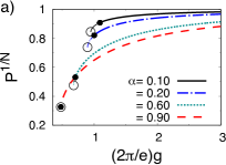
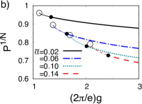
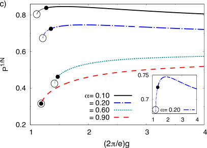
Figure 9: Geometric mean purity $\mathcal{P}^{1/N}$, for $N=150$ , as a function of $g$. The solid dot corresponds to the phase transition $\mathcal{F}_{v}(V_{sc})=\mathcal{F}_{v}(0)$ while the open circles mark the disappearance of the self-consistent solution. a) Conventional dissipation for different values of $\alpha$. b) Unconventional dissipation for different values of $\widetilde{\alpha}$. c) Frustrated case for the ratio $\widetilde{\alpha}/\alpha=0.3$. The inset is a zoom for the case $\alpha=0.2.$

V.2 Entanglement

In this section we analyze an entanglement measure to describe the non-classical correlations present in the quantum phase model with dissipative frustration. Specifically, we discuss the behavior of the logarithmic negativity $E_{\mathcal{N}}$, a suitable entanglement measure to characterize Gaussian states Adesso and Illuminati (2007); Vidal and Werner (2002).
Before we discuss the logarithmic negativity and the results for our system, a remark is needed. To compute $E_{\mathcal{N}}$ we use a Gaussian density matrix $\hat{\rho}_{sc}$, see Eqs. (24) and (25). The results we obtain in this way naturally can be different from the exact measure of the quantum phase model with the cosine interaction having non-Gaussian correlations. Since $E_{\mathcal{N}}$ fails to be superadditive, the results obtained with the Gaussian state do not represent a lower bound and can overestimate the amount of entanglement Wolf et al. (2006). However, $E_{\mathcal{N}}$ is a simple and straightforward quantity to compute and it can provide a first, rough estimate of the possible behavior of the entanglement in our problem.
The logarithmic negativity is based on the Peres-Horodecki criterion (or Positive Partial Transpose, PPT) Peres (1996); Horodecki et al. (1996) which states that if the global density matrix $\hat{\rho}$ for two combined subsystems $A$ and $B$ is separable (= no entanglement but only classical correlations), then the partial transpose density matrix respect to one of the two subsystems, for instance $\hat{\rho}^{T_{A}}$, has still positive eigenvalues. Hence, the amount of negativeness of the eigenvalues of $\hat{\rho}^{T_{A}}$ can be considered as a measure of the non-separability between $A$ and $B$, viz. entangled states are present. Following this criterion, one defines the logarithmic negativity in our case as

$$E_{\mathcal{N}}\left[\hat{\rho}\right]=\log_{2}\left(||\hat{\rho}^{T_{A}}||_{1}\right)=\log_{2}(1-2\sum_{\lambda_{k}<0}\lambda_{k}[\hat{\rho}^{T_{A}}])\,,$$ (31)

where $\lambda_{k}[\hat{\rho}^{T_{A}}]$ are the eigenvalues of $\hat{\rho}^{T_{A}}$ and $||M||_{1}$ denotes the trace norm of a matrix $M$, $||M||_{1}=\text{tr}(\sqrt{M^{\dagger}M})$ and corresponds to the sum of the absolute values of its eigenvalues . The PPT criterion is a sufficient condition, implying that even for $E_{\mathcal{N}}=0$, the two subsystems can still have some entanglement Patanè et al. (2007).

We calculate the logarithmic negativity $E_{\mathcal{N}}[\hat{\rho}_{sc}]$ for our system using the correlation covariance matrix Simon (2000); Vidal and Werner (2002); Adesso and Illuminati (2007). A more detailed discussion of the formalism is given in Appendix C, illustrating the case of two coupled oscillators.

We introduce the canonical conjugated variables $\hat{q}_{n}=\hat{Q}_{n}/(2e)$, i.e. the scaled charge operators on each superconducting island forming the chain, with the commutation relation $[\hat{\varphi}_{n},\hat{q}_{m}]=i\delta_{nm}$. We also define the vector

$$\hat{R}=\left(\hat{R}_{1},\hat{R}_{2},\dots,\hat{R}_{N}\right)^{T}\,,$$ (32)

with $\hat{R}_{n}=(\hat{\varphi}_{n},\hat{q}_{n})$. The full symmetric covariance matrix $\hat{\sigma}[\hat{\rho}_{sc}]$ of size $(N\times N)$ is formed by the block elements $(2\times 2)$ that read

$$\hat{\sigma}_{nm}[\hat{\rho}_{sc}]=\langle\hat{R}_{l}\hat{R}_{m}+\hat{R}_{m}\hat{R}_{l}\rangle/2\,.$$ (33)

The correlation functions are given by

$$\langle\varphi_{n}^{2}\rangle =\langle\varphi^{2}\rangle=\frac{1}{N}\sum_{k=1}^{N-1}\langle{\left|\varphi_{k}\right|}^{2}\rangle$$ (34)

$$\langle\varphi_{l}\varphi_{m}\rangle =\frac{1}{N}\sum_{k=1}^{N-1}\cos\left(\frac{2\pi}{N}k(m-l)\right)\langle{\left|\varphi_{k}\right|}^{2}\rangle,$$ (35)

and similar expressions for $\langle q_{n}^{2}\rangle=\langle q^{2}\rangle\propto\langle\dot{\varphi}^{2}\rangle$ and $\langle q_{n}q_{m}\rangle\propto\langle\dot{\varphi}_{n}\dot{\varphi}_{m}\rangle$, whereas we have $\langle\hat{\varphi}_{n}\,\hat{q}_{m}\rangle=0$.

After having partitioned the superconducting Josephson chain in two subsystems formed by the local variables $n_{A}=1,\dots,N_{A}$ and $n_{B}=1,\dots,N_{B}$, it is possible to show that the covariance matrix $\hat{\sigma}[\hat{\rho}_{sc}^{T_{A}}]$ associated to $\hat{\rho}^{T_{A}}_{sc}$ is easily obtained by time reversal symmetry operations Simon (2000), viz. by inverting all momenta of subsystem $A$, namely

$$\hat{\sigma}[\hat{\rho}_{sc}]\rightarrow\hat{\sigma}[\hat{\rho}_{sc}^{T_{A}}]\quad\mbox{with}\quad\langle q_{n_{A}}q_{m_{B}}\rangle\rightarrow-\langle q_{n_{A}}q_{m_{B}}\rangle\,,$$ (36)

and leaving unmodified the products in each subsystem $\langle q_{n_{A}}q_{m_{A}}\rangle$ and $\langle q_{n_{B}}q_{m_{B}}\rangle$. Finally, the connection between the logarithmic negativity and the covariance matrix of the partial transpose matrix $\hat{\sigma}[\hat{\rho}_{sc}^{T_{A}}]$ is given by the formula Serafini (2006)

$$E_{\mathcal{N}}[\hat{\rho}_{sc}]=-\sum_{k}\log_{2}\left(\min[1,(2c_{k})]\right)\,,$$ (37)

where the quantities $\{c_{1},c_{2},...,c_{N}\}$ are the symplectic eigenvalues (spectrum) associated to the covariance matrix $\hat{\sigma}[\hat{\rho}_{sc}^{T_{A}}]$. The symplectic spectrum is computed by finding the real eigenvalues of the real symmetric matrix $\hat{S}=-i\mathcal{O}\hat{\sigma}[\hat{\rho}_{sc}^{T_{A}}]$, namely the product of the covariance matrix with the symplectic block diagonal matrix

$$\mathcal{O}=\bigoplus_{n=1}^{N}\left(\begin{array}[]{cc}0&1\\ -1&0\end{array}\right)\,.$$ (38)

In the diagonal form, the matrix $\hat{S}$ reads $\text{diag}\{\pm c_{1},\pm c_{2},...,\pm c_{N}\}$ Serafini (2006) (see Appendix C for more details).

The symplectic eigenvalues $\{c_{k}\}$ are continuous functions of the correlation functions of the system.

We find that the symplectic spectrum and hence the logarithmic negativity does not vary with $g$ without coupling with the environment. This results can be understood by scaling analysis of the symplectic spectrum as a function of the normal modes. In other words, for Gaussian states, the degree of quantum correlations between coupled harmonic oscillators (viz. the local phases) does not depend on the amount of the phase-difference quantum fluctuations $\sim{\langle\Delta\hat{\varphi}^{2}\rangle}_{0}\sim 1/\sqrt{g}$. By contrast, when the chain is coupled to the environment, we find that a such dissipation interaction always yields a decreasing of the entanglement with respect to the value of the isolated system.

Generally, the logarithmic negativity depends on the specific configuration for the partition of the system in two subsystems $A$ and $B$ since the correlation functions between different sites are long-ranged, see Eq. (35). Here, as example of results, in Fig. 10, we present the case for the logarithmic negativity by dividing the periodic lattice (ring) formed by $N=9$ sites partitioned in two compact subsystems of size $N_{A}=4$ and $N_{B}=5$. Our qualitative results and conclusions do not depend on this specific choice and further configurations are discussed in Appendix D.

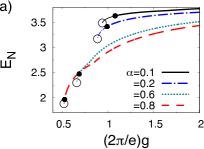
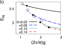
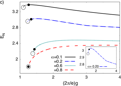
Figure 10: Logarithmic negativity for $N=9$ sites and subsystem sizes $N_{A}=4,N_{B}=5$ as a function of $g$. The solid dot corresponds to $\mathcal{F}_{v}(V_{sc})=\mathcal{F}_{v}(0)$ while the open circles mark the disappearance of the self-consistent solution Eq. (23). a) Conventional dissipation for different coupling of $\alpha$. b) Unconventional dissipation for different couplings $\widetilde{\alpha}$. c) Frustrated dissipation with the ratio $\widetilde{\alpha}/\alpha=0.3$. The inset is a zoom for the case $\alpha=0.2.$

Fig. 10(a) and (b) show the logarithmic negativity as a function of $g$ when only one type of dissipative interaction is affecting the system, $\widetilde{\alpha}=0$ or $\alpha=0$ respectively. The global behavior is very similar to the results obtained for the purity. However, the logarithmic negativity shows a non-continuous behavior of the derivative, with kinks appearing for lower values of $g$. This can be explained by considering the formal definition of $E_{\mathcal{N}}$: decreasing $g$, the kinks correspond to the point where a symplectic eigenvalue becomes less than the fixed threshold $(c_{k}<1/2)$, yielding an additional term in the sum of Eq. (37).

Finally, we report the most interesting case of dissipative frustration with $\widetilde{\alpha}/\alpha=0.3$ in Fig. 10(c). As for the purity, for a given ratio $\widetilde{\alpha}/\alpha<1$, the logarithmic negativity can display a non-monotonic behavior for not too large values of the dissipative interaction.

VI Summary

To summarize, we studied a 1D quantum phase model with dissipative frustration defined as a system coupled to the environment through two non-commuting observables, namely the phase and its conjugated operator, Fig. 1(a). We showed that this system can be readily implemented using one dimensional Josephson junction chains formed by superconducting islands connected by Josephson coupling. In these systems, the local phases and charges are the canonically conjugated variables. The conventional (phase) dissipation arises from the shunt resistances in parallel between two neighboring islands whereas the unconventional (charge) is related to the resistance connecting the local capacitance to the ground, Fig. 1(b). When the two dissipative interactions affect separately the system, they yield quenching of, respectively, the quantum phase fluctuations or quantum charge fluctuations. When both two dissipative interaction are present, frustration emerges due to the uncertainty relation that sets a lower bound to the product of the two fluctuations.

Quantum fluctuations play a crucial role in the quantum phase transition occurring the 1D quantum phase model. This corresponds to the superconductor vs insulator phase transition in the Josephson chain, associated to the presence of phase ordering or not. Using the Self Consistent Harmonic Approximation (SCHA), we derive the qualitative phase diagram of the system under the influence of the dissipation. The dissipative frustration operating in the system leads to a non-monotonic behavior of the quantum fluctuations Kohler and Sols (2006); Rastelli (2016) which translates into the non-monotonic behavior of the critical line in the phase diagram at fixed ratio of the two dissipative coupling strengths.

The dissipative frustration has a genuine quantum origin since it is related to the non-commutativity of quantum operators. Hence, we analyzed the effects of the dissipative frustration in the average quantities characterizing the state of the system. In particular, we discussed two quantum thermodynamical quantities, the purity and the entanglement measure of the logarithmic negativity, which have no analog in classical systems. We found that, within the SCHA approach, both quantities show a non-monotonic behavior approaching the critical point associated to the dissipative phase transition.

In conclusion, our results for a specific system demonstrate that dissipative frustration can lead to interesting effects and novel features in the physics of open quantum many body systems.

VII Acknowledgements

The authors thank Luigi Amico, Denis Basko, Daniel Braun, Rosario Fazio and Nils Schopohl for useful discussions. Sabine Andergassen acknowledges the Wolfgang Pauli Institute for the kind hospitality. We acknowledge financial support from the Deutsche Forschungsgemeinschaft (DFG) through ZUK 63, SFB 767 and the Zukunftskolleg, and by the MWK-RiSC program.

Appendix A Unconventional or charge dissipation in the equations of motions

In this appendix we discuss the dissipation obtained by coupling a superconducting island to the ground via an impedance formed by the series of capacitances. We directly include capacitances in the equation whereas the resistive elements are taken into account by a standard Caldeira-Leggett approach, i.e. introducing a discrete line formed by capacitances $C_{g}$ and inductances $L_{g}$, as shown in Fig. 11. This line is formed by $M$ elements. We will consider the limit $M\rightarrow\infty$ to recover the full dissipative ohmic behavior. To simplify the notation, we set the local superconducting phase in the island of the Josephson junction chain $\varphi_{n}\rightarrow\varphi$.

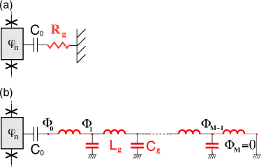
Figure 11: (a) One superconducting island of the Josephson junction chain with local phase $\varphi$ connected to the ground through the series formed by the capacitance $C_{0}$ and the resistance $R_{g}$. (b) Equivalent circuit simulating the dissipation by using the Caldeira-Leggett model, with a transmission line formed by discrete elements, that contains the inductance $L_{g}$ and the capacitance $C_{g}$, with the characteristic impedance $R_{g}=\sqrt{L_{g}/C_{g}}$.

Referring to Fig. 11(b), we discuss the circuit using the equations of motion for a lumped number of circuit elements Devoret (2002). We use the phase nodes variables $\phi_{m}$, with $m=0,\dots,M$, with the boundary condition $\phi_{M}=0$. We start by the Kirchoff’s equation for the energy conservation at each node $m=1,\dots,M-1$ of the circuit Fig. 11(b),

$$C_{g}\frac{d^{2}\phi_{m}}{dt^{2}}=-\frac{1}{L_{g}}\left(2\phi_{m}-\phi_{m-1}-\phi_{m+1}\right)\,.$$ (39)

Introducing the vector $\vec{\phi}^{\prime}=(\phi_{1},\phi_{2},\dots,\phi_{m},\dots,\phi_{M-1})$ and the frequency $\omega_{g}^{2}=1/(L_{g}C_{g})$, the previous equation can be cast in the matrix form

$$\frac{d^{2}\vec{\phi}^{\prime}}{dt^{2}}\!\!=\!-\omega_{g}^{2}\left(\begin{array}[]{ccccc}2&-1&0&\dots&\dots\\ -1&2&-1&0&\dots\\ 0&-1&2&-1&\dots\\ \dots&\dots&\dots&\dots&-1\\ \dots&\dots&0&-1&2\end{array}\right)\vec{\phi}^{\prime}+\omega_{g}^{2}\left[\begin{array}[]{c}\phi_{0}\\ 0\\ \dots\\ 0\end{array}\right]\,.$$ (40)

The eigenvectors, $e_{k}(m)=\sqrt{2/M}\sin\left[\pi km/M\right]$ of the matrix $\bar{\bar{M}}$, with $m=1,\dots,M-1$, span the matrix $\bar{\bar{M}}=\bar{\bar{U}}\bar{\bar{D}}{\bar{\bar{U}}}^{-1}$, where $\bar{\bar{D}}$ is the diagonal form and $\bar{\bar{U}}$ ($\bar{\bar{U}}^{-1}$) contains the (normalized) eigenvectors. This corresponds to the unitary transformation $\phi_{m}=\sum_{k=1}^{M-1}e_{k}(m)\Phi_{k}$ for $m=1,\dots,M-1$. Eq. (40) reads then in terms of the normal modes $\Phi_{k}$

$$\frac{d^{2}\Phi_{k}}{dt^{2}}=-\Omega_{k}^{2}\Phi_{k}+\omega_{g}^{2}\sum_{k=1}^{M-1}\epsilon_{k}\phi_{0}\,,$$ (41)

with the spectrum $\Omega_{k}=2\omega_{g}\sin\left[\pi k/(2M)\right]$ and $\epsilon_{k}=e_{k}(1)=\sqrt{2/M}\sin\left[\pi k/M\right]$. The solution of Eq. (41) is given by

$$\Phi_{k}(t) = \Phi_{k}^{(0)}(t)+\frac{\omega_{g}^{2}}{\Omega_{k}}\epsilon_{k}\int^{t}_{t_{0}}\!\!\!dt^{\prime}\sin\left[\Omega_{k}(t-t^{\prime})\right]\phi_{0}(t^{\prime})$$ (42)

$$= \Phi_{k}^{(0)}(t)+\frac{\omega_{g}^{2}}{\Omega_{k}^{2}}\epsilon_{k}\left[\phi_{0}(t)-\cos\left[\Omega_{k}(t-t_{0})\right]\phi_{0}(t_{0})\right]$$

$$- \frac{\omega_{g}^{2}}{\Omega_{k}^{2}}\epsilon_{k}\int^{t}_{t_{0}}\!\!\!dt^{\prime}\cos\left[\Omega_{k}(t-t^{\prime})\right]\frac{d\phi_{0}(t^{\prime})}{dt^{\prime}}\,,$$

with $\Phi_{k}^{(0)}(t)$ being the solution of the associated homogeneous Eq. (41). Then, we write the dynamics equation for the node $m=0$

$$C_{0}\frac{d^{2}\left(\phi_{0}-\varphi\right)}{dt^{2}} = -\frac{1}{L_{g}}\left(\phi_{0}-\phi_{1}\right)$$ (43)

$$= -\frac{\phi_{0}}{L_{g}}+\frac{1}{L_{g}}\sum_{k=1}^{M-1}\epsilon_{k}\Phi_{k}(t)\,.$$

Inserting the solution (42) for $\Phi_{k}(t)$ into Eq. (43), after some algebra, we obtain

$$C_{0}\frac{d^{2}\left(\phi_{0}-\varphi\right)}{dt^{2}}=-\frac{\phi_{0}}{ML_{g}}+\delta I_{0}(t)-\int^{+\infty}_{-\infty}\!\!\!\!\!\!\!dt^{\prime}Y(t-t^{\prime})\frac{d\phi_{0}(t^{\prime})}{dt^{\prime}}\,,$$ (44)

where we set the initial time $t_{0}\rightarrow-\infty$ and $\delta I_{0}(t)$ is a time function depending on the initial conditions. This function corresponds to the noise and we can ignore it for the rest of the discussion. The relevant quantity appearing in Eq. (44) is the response function given by

$$Y(t)=\theta(t)\frac{2}{ML_{g}}\sum_{k=1}^{M-1}\left(1-\frac{\Omega_{k}^{2}}{4\omega_{g}^{2}}\right)\cos\left[\Omega_{k}t\right]\,.$$ (45)

Finally, we take the thermodynamic limit for the number of the elements in the line $M\rightarrow\infty$ such that the real part of the Fourier transform of the response function $Y(t)$, associated to the dissipation, becomes finite and reads

$$\lim_{M\rightarrow\infty}\mbox{Re}\left[Y(\omega)\right]=(1/R_{g})f_{c}(\omega)\,,$$ (46)

with the high frequency cutoff $\sim\omega_{g}$ that we neglect hereafter to simplify the notation. Omitting the noise and using the Markovian approximation (viz. the decay rate $\sim 1/\omega_{g}$ of the function $Y(t)$ much larger than the time scale of the evolution of the phases), we have

$$\frac{d^{2}\phi_{0}}{dt^{2}}=-\frac{1}{\tau_{g}}\frac{d\phi_{0}(t)}{dt}+\frac{d^{2}\varphi}{dt^{2}}\,,$$ (47)

with $\tau_{g}=C_{0}R_{g}$. We then consider the particular solution $\phi_{0}(t)=\int_{-\infty}^{t}\!\!\!dt^{\prime}\exp\left[-(t-t^{\prime})/\tau_{g}\right]d\varphi(t^{\prime})/dt^{\prime}$ with the property

$$\frac{d\phi_{0}(t)}{dt}=\frac{d\varphi(t)}{dt}-\frac{1}{\tau_{g}}\int_{-\infty}^{t}\!\!\!\!\!\!dt^{\prime}\exp\left[-(t-t^{\prime})/\tau_{g}\right]\frac{d\varphi(t^{\prime})}{dt^{\prime}}\,.$$ (48)

In this way we can show that

$$\frac{d^{2}\left(\phi_{0}-\varphi\right)}{dt^{2}}=-\frac{1}{\tau_{g}}\frac{d\varphi(t)}{dt}+\frac{1}{\tau_{g}^{2}}\int_{-\infty}^{t}\!\!\!\!\!\!\!dt^{\prime}e^{-\frac{t-t^{\prime}}{\tau_{g}}}\frac{d\varphi(t^{\prime})}{dt^{\prime}}\,.$$ (49)

In the final step, we recover the index for each element $\varphi\rightarrow\varphi_{n}$ and write the equation for the phase $\varphi_{n}$ (in the Markovian limit) of the 1DJJ shown Fig. 1 as

$$\frac{d^{2}\left(\varphi_{n}-\phi_{0}\right)}{dt^{2}}=-\omega_{0}^{2}\left(2\varphi_{n}-\varphi_{n-1}-\varphi_{n+1}\right)-\gamma\frac{d\varphi_{n}}{dt}\,,$$ (50)

with $\omega_{0}=\sqrt{E_{C}E_{J}}/\hbar$ and $\gamma=1/(R_{s}C_{0})$. Using the main result Eq. (49), the Fourier transform of Eq. (50) reads

$$-\frac{\omega^{2}\varphi_{n}(\omega)}{1+i\tau_{g}\omega}=-\omega_{0}^{2}\left[2\varphi_{n}-\varphi_{n-1}-\varphi_{n+1}\right]_{\omega}-i\gamma\omega\varphi_{n}(\omega)$$ (51)

in which we are interested only to the l.h.s. describing the effect of the unconventional (charge) dissipation in frequency space. Thus, we conclude that the unconventional dissipation corresponds to a damped (imaginary) mass in the equation of motion of the local phases $\varphi_{n}$.

We finally observe that, using the Wick’s rotation from real frequency $\omega$ to Matsubara frequency $-i\omega_{\ell}$ and restoring the capacitance (mass) in the l.h.s. of Eq. (51), we get

$$\frac{C_{0}\omega^{2}_{\ell}}{1+\tau_{g}\omega_{\ell}}\sim\widetilde{F}_{\ell}\,\,\omega_{\ell}^{2}\,,$$ (52)

where the propagator $\widetilde{F}_{\ell}$ is given by Eq. (10) with the cutoff function $f_{c}=1$ and $\omega_{\ell}>0$. A rigorous derivation will be given in the following Appendix B.

Appendix B Unconventional or charge dissipation with the path integral in the imaginary time

In this appendix we derive the unconventional or charge dissipation introduced in the main text, in the path integral formalism in imaginary time

As first step, we recall the Lagrangian in the imaginary time of the Josephson junction chains with each junction shunted by the resistance $R_{s}$,

$$\mathcal{S}_{JJ} = \sum_{n=0}^{N-1}\frac{1}{2}\int_{0}^{\beta}\!\!\!\!\int_{0}^{\beta}\!\!d\tau d\tau^{\prime}\,F(\!\tau\!-\!\tau^{\prime})\,{\left|\Delta\varphi_{n}(\tau)-\Delta\varphi_{n}(\tau^{\prime})\right|}^{2}$$ (53)

$$- \sum_{n=0}^{N-1}E_{J}\cos\left(\Delta\varphi_{n}(\tau)\right)\,,$$

where $E_{J}$ is the Josephson energy and the function $F(\tau)$ encoding the ohmic dissipation of $R_{s}$ refers to Eq. (8) discussed in the main text. Then we assume that each local superconducting island $n$ is coupled to an external bath (external impedance) leading to the general form of the Lagrangian

$$\mathcal{S}=\mathcal{S}_{JJ}+\int^{\beta}_{0}\!\!\!\!d\tau\sum_{n=0}^{N-1}\mathcal{L}_{0}^{(n)}\,.$$ (54)

The external impedance is formed by the capacitance $C_{0}$ and a resistance $R_{g}$, as depicted in Fig. 11(a). The dissipative element $R_{g}$ is described by the Caldeira-Leggett model, viz. as an ensemble of $M$ discrete elements forming a transmission line, as depicted in the Fig. 11(b). In the thermodynamic limit $M\rightarrow\infty$, such a line is equivalent to the resistance $R_{g}$, as we show in the following.

To construct the Lagrangian we have to consider the electrostatic energy associated to each link containing a capacitance and the associated inductive energy Devoret (2002). The result is

$$\frac{\mathcal{L}_{0}^{(n)}}{\mu_{0}} = \frac{C_{0}}{2}{\left(\dot{\varphi}_{n}-\dot{\phi}_{0}^{(n)}\right)}^{2}+\frac{{\left(\phi_{0}^{(n)}-\phi_{1}^{(n)}\right)}^{2}}{2L_{g}}$$ (55)

$$+ \!\!\sum_{m=1}^{M-1}\!\!\left[\frac{C_{g}}{2}{\left(\dot{\phi}_{m}^{(n)}\right)}^{2}\!\!\!+\!\frac{{\left(\phi_{m+1}^{(n)}-\phi_{m}^{(n)}\right)}^{2}}{2L_{g}}\!\right],$$

with $\mu_{0}=\Phi_{0}^{2}/(4\pi^{2})$ and $\Phi_{0}=h/(2e)$ the flux quantum. Then we express the partition function of the whole system in the imaginary time path integral formalism Weiss (2012)

$$Z = \!\!\prod_{n,m}\!\oint\!D[\varphi_{n}(\tau)]e^{-\frac{\mathcal{S}_{JJ}}{\hbar}}\!\!\oint\!D[\phi_{m}^{(n)}(\tau)]e^{-\frac{1}{\hbar}\sum_{n=0}^{N-1}\int\limits_{0}^{\beta}d\tau\mathcal{L}_{0}^{(n)}}$$ (56)

$$\equiv \prod_{n}\oint D[\varphi_{n}(\tau)]e^{-\frac{\mathcal{S}_{JJ}}{\hbar}}\,\,\,\mbox{F}_{ch}[\varphi]\,.$$

Hereafter, we focus only on one superconducting island $n$ described by the phase $\varphi_{n}$, and to simplify the notation we drop the index $n$. Hence, we consider the Lagrangian $\mathcal{L}_{0}$ (without index n) in Eq. (55). Now can diagonalize the part containing the transmission line for the phases $m=1,\dots,M-1$ via the unitary transformation introduced in the previous Appendix A. Then the ensemble of the harmonic modes $\Phi_{k}$ represents the effective bath affecting the phase $\phi_{0}$ and that eventually becomes equivalent to a dissipative resistance. Only the phase $\phi_{0}$ is directly coupled capacitively to the superconducting phase $\varphi$ of the local island forming the 1DJJ. Thus we obtain

$$\mbox{F}_{ch}[\varphi] = \oint D[\phi_{0}(\tau)]e^{-\frac{1}{\hbar}\int\limits_{0}^{\beta}d\tau\left[\frac{\mu_{0}C_{0}}{2}{\left(\dot{\varphi}-\dot{\phi}_{0}\right)}^{2}\right]}$$ (57)

$$\prod_{k=1}^{M-1}\oint D[\Phi_{k}(\tau)]e^{-\frac{1}{\hbar}\int\limits_{0}^{\beta}d\tau\mathcal{L}_{g}}\,,$$

where $\mathcal{L}_{g}$ is given by

$$\frac{\mathcal{L}_{g}}{\mu_{0}}=\frac{\phi_{0}^{2}}{2L_{g}}-\frac{\phi_{0}}{L_{g}}\sum_{k}\epsilon_{k}\Phi_{k}+\frac{C_{g}}{2}\sum_{k=1}^{M-1}\left[\dot{\Phi}_{k}^{2}+\frac{\Omega_{k}^{2}}{2}\Phi_{k}^{2}\right]$$ (58)

and the spectrum $\Omega_{k}^{2}$ and $\epsilon_{k}$ are defined above. In order to derive the final effective functional for the phase $\varphi$, we have first to integrate out the harmonic modes $\Phi_{k}$ and then the phase variable $\phi_{0}$ directly coupled to the superconducting phase $\varphi$ via the capacitance $C_{0}$. Using the Matsubara Fourier transformation $\Phi_{k}(\tau)=\sum_{k}\Phi_{\ell}^{(k)}\exp(i\omega_{\ell}\tau)$ and $\phi_{0}(\tau)=\sum_{k}\phi_{\ell}^{(0)}\exp(i\omega_{\ell}\tau)$, with $\omega_{\ell}=2\pi\ell/\beta$ ($\ell$ integer), we express the action $\mathcal{L}_{g}$ as

$$\frac{1}{\hbar}\int_{0}^{\beta}\!\!\!\!d\tau\mathcal{L}_{g}=\frac{\beta\mu_{0}}{\hbar L_{g}}\sum_{\ell=0}^{\infty}\left(1-\frac{\delta_{\ell,0}}{2}\right){\left|\phi_{\ell}^{(0)}\right|}^{2}$$ (59)

$$- \frac{\beta\mu_{0}}{\hbar L_{g}}\sum_{k}^{M-1}\epsilon_{k}\left[\phi_{0}^{(0)}\Phi_{0}^{(k)}+\sum_{\ell=0}^{\infty}\left(\phi_{\ell}^{(0)}\Phi_{\ell}^{(k)*}+\phi_{\ell}^{(0)*}\Phi_{\ell}^{(k)}\right)\right]$$

$$+ \frac{\beta C_{g}\mu_{0}}{\hbar}\sum_{k=1}^{M-1}\sum_{\ell=0}^{\infty}\left[\omega_{\ell}^{2}+\Omega_{k}^{2}\left(1-\frac{\delta_{\ell,0}}{2}\right)\right]{\left|\Phi_{\ell}^{(k)}\right|}^{2}$$

to be inserted in the path integral Eq. (57) with the metric Kleinert (2009); Weiss (2012)

$$\!\oint\!\!D[\Phi_{k}(\tau)]\!\rightarrow\!\!\int\!\!\frac{d\Phi_{0}^{(k)}}{\sqrt{2\pi\hbar\beta/(\mu_{0}C_{g})}}\prod_{\ell=1}^{\infty}\!\int\!\!\!\ \frac{d\Phi_{\ell}^{(k),Re}d\Phi_{\ell}^{(k),Im}}{\pi\hbar/(\beta\mu_{0}C_{g}\omega_{\ell}^{2})},$$ (60)

with $\Phi_{\ell}^{(k),Re}$ and $\Phi_{\ell}^{(k),Im}$ the real and imaginary part of $\Phi_{\ell}^{(k)}$ $(\ell\neq 0)$, respectively. After performing the Gaussian integral, we derive the effective action for the phase $\Phi_{M}$

$$\mbox{F}(\phi) = \oint D[\phi_{0}(\tau)]e^{-\frac{1}{\hbar}\int\limits_{0}^{\beta}d\tau\left[\frac{\mu_{0}C_{0}}{2}{\left(\dot{\varphi}-\dot{\phi}_{0}\right)}^{2}\right]}$$ (61)

$$\left[\prod_{k=1}^{M-1}Z_{h}(\Omega_{k})\right]e^{-\frac{1}{\hbar}\Delta S_{eff}[\phi_{0}]},$$

where $Z_{h}(\Omega)$ is the partition function of a harmonic oscillator of frequency $\Omega$ that we omit hereafter, and $\Delta S_{eff}[\phi_{0}]$ the effective action for the phase $\phi_{0}$ which reads in Matsubara space

$$\Delta S_{eff}[\phi_{0}]\!=\!\beta\mu_{0}\!\sum_{\ell=0}^{\infty}\left[\frac{1}{L_{g}M}\!\left(\!1\!-\!\frac{\delta_{\ell,0}}{2}\!\right)\!+\omega_{\ell}\mbox{Y}_{\ell}\right]{\left|\phi_{\ell}^{(0)}\right|}^{2}\,.$$ (62)

In Eq. (62), the first term represents an effective inductance for the phase $\phi_{0}$ that vanishes in the limit $M\rightarrow\infty$, whereas the relevant term is the second one with the function

$$\mbox{Y}_{\ell}=\frac{2\omega_{\ell}}{ML_{g}}\sum_{k=1}^{M-1}\left(1-\frac{\Omega_{k}^{2}}{4\omega_{g}^{2}}\right)\frac{1}{\omega_{\ell}^{2}+\Omega_{k}^{2}}.\\$$ (63)

Note the similarity of $\mbox{Y}_{\ell}$ in Eq. (63) with Eq. (45) for the response function (admittance) of the transmission line. With some algebra, setting $R_{g}=\sqrt{L_{g}/C_{g}}$, we cast $\mbox{Y}_{\ell}$ in the following form

$$\mbox{Y}_{\ell} = \left(1/R_{g}\right)\frac{2}{\pi}{\left[x_{\ell}\,\frac{\pi}{2M}\sum_{k=1}^{M-1}\frac{1-\sin^{2}\left(\frac{\pi k}{2M}\right)}{x^{2}_{\ell}+\sin^{2}\left(\frac{\pi k}{2M}\right)}\right]}_{x_{\ell}=\frac{\omega_{\ell}}{2\omega_{g}}}$$

_(M→∞) $$= \left(1/R_{g}\right)\frac{2}{\pi}{\left[x_{\ell}\int_{0}^{\frac{\pi}{2}}\!\!\!d\theta\frac{1-\sin^{2}(\theta)}{x^{2}_{\ell}+\sin^{2}(\theta)}\right]}_{x_{\ell}=\frac{\omega_{\ell}}{2\omega_{g}}}$$ (64)

$$= \left(1/R_{g}\right)f_{c}\left(\omega_{\ell}\right),$$

where in the second line we have taken the limit $M\rightarrow\infty$ replacing the sum with the continuous integral. $x_{\ell}=\omega_{\ell}/(2\omega_{g})$ corresponds to the cutoff function with high frequency $\omega_{c}=2\omega_{g}$. For the specific choice of the circuit discussed here leading to Eq. (64), we get $f_{c}(\omega_{\ell})=\sqrt{1+x^{2}_{\ell}}-x_{\ell}$. However, details of the specific form of the cutoff functions are irrelevant for the results analyzed in the main text. In the limit in which $\omega_{c}$ represents the high frequency involved in the problem, we expect only logarithmic corrections to the average phase difference fluctuations, see Eq. (19).

Summarizing we have shown that

$$\Delta S_{eff}[\phi_{0}]=\beta\frac{\hbar}{2\pi}\frac{R_{q}}{R_{g}}\sum_{\ell=1}^{\infty}\omega_{\ell}f_{c}(\omega_{\ell}){\left|\phi_{\ell}^{(0)}\right|}^{2}\,,$$ (65)

where $\mu_{0}=\Phi_{0}/(2\pi)=R_{q}\hbar/(2\pi)$. Indeed, this is exactly the same form as for the dissipative function describing a shunt resistance for the Josephson junction phase difference, see Eq. (8) for which we have given, en passant, a demonstration.

In the last part, we have to perform the integral in Eq. (61) with the action Eq. (65), with the use of the metric

$$\!\oint\!\!D[\phi_{0}(\tau)]\!\rightarrow\!\!\int\!\!\frac{d\phi_{0}^{(0)}}{\sqrt{2\pi\hbar\beta/(\mu_{0}C_{0})}}\prod_{\ell=1}^{\infty}\!\int\!\!\!\ \frac{d\phi_{\ell}^{(0),Re}d\phi_{\ell}^{(0),Im}}{\pi\hbar/(\beta\mu_{0}C_{0}\omega^{2}_{\ell})}.$$ (66)

The Gaussian integral is then carried out using the Matsubara frequency representation, which yields

$$\mbox{F}(\phi) \sim\exp\left[\frac{\hbar\beta}{E_{C}}\sum_{\ell=1}^{\infty}\frac{\hbar}{2\pi}\left(\frac{\omega_{\ell}^{2}}{1+\omega_{\ell}\tau_{g}f_{c}(\omega_{\ell})}\right){\left|\varphi_{\ell}\right|}^{2}\right]\,.$$ (67)

The latter expression corresponds to the part containing the unconventional or charge damping kernel $\tilde{F}(\tau-\tau^{\prime})$ in the total action of the system for each local phase $\varphi_{n}$ in Eq. (II.2), with the propagator given by $\tilde{F}_{\ell}$ in Eq. (10).

Appendix C Covariance matrix and logarithmic negativity

To illustrate the method used in Sec. V to compute the logarithmic negativity from the covariance matrix, we discuss in this appendix the simple example of two coupled oscillators. In particular, we calculate the symplectic eigenvalues and show how it is related to the Heisenberg uncertainty principle. We refer to the works Refs. Adesso and Illuminati (2007); Vidal and Werner (2002); Simon (2000); Serafini (2006) for extended discussions.

We consider two harmonic oscillators described by the two position and momentum operators which define the vector

$$\hat{R}=(\hat{R}_{0},\hat{R}_{1})=(\hat{x}_{0},\hat{p}_{0},\hat{x}_{1},\hat{p}_{1})^{T}\,,$$ (68)

with the Hamiltonian

$$\hat{H}=\frac{1}{2m}(\hat{p}_{0}^{2}+\hat{p}_{1}^{2})+\frac{k_{0}}{2}(\hat{x}_{0}^{2}+\hat{x}_{1}^{2})+\frac{k}{2}(\hat{x}_{0}-\hat{x}_{1})^{2}.$$ (69)

The corresponding commutator relation reads

$$[\hat{R}_{i},\hat{R}_{j}]=i\hbar\delta_{ij}\left(\begin{array}[]{cc}0&1\\ -1&0\end{array}\right).$$ (70)

The $(4\times 4)$ matrix

$$\mathcal{O}=\bigoplus_{n=0}^{1}\left(\begin{array}[]{cc}0&1\\ -1&0\end{array}\right)\,$$ (71)

is the symplectic matrix, which is invariant under symplectic transformations $S^{T}\mathcal{O}S=\mathcal{O}$, with $S\in\text{Sp}(4,\mathbb{R})$ denoting the symplectic group. The covariance matrix reads

$$\sigma=\left(\begin{array}[]{cccc}\langle\hat{x}_{0}^{2}\rangle&0&\langle\hat{x}_{0}\hat{x}_{1}\rangle&0\\ 0&\langle\hat{p}_{0}^{2}\rangle&0&\langle\hat{p}_{0}\hat{p}_{1}\rangle\\ \langle\hat{x}_{0}\hat{x}_{1}\rangle&0&\langle\hat{x}_{1}^{2}\rangle&0\\ 0&\langle\hat{p}_{0}\hat{p}_{1}\rangle&0&\langle\hat{p}_{1}^{2}\rangle\end{array}\right).$$ (72)

The Heisenberg uncertainty principle is equivalent to the condition that the eigenvalues of the matrix given by the sum of $\sigma$ and $(i\hbar/2)\mathcal{O}$ are always positive or zero, namely

$$\left[\sigma+i\frac{\hbar}{2}\mathcal{O}\right]\geq 0\,.$$ (73)

In other words, the l.h.s. of Eq. (73) has to be positive semi-definite such that the matrix $\sigma$ has a physical meaning. As the covariance matrix is positive and symmetric, according to the Williamson’s theorem, it is always possible to cast it in a diagonal form using a symplectic transformation

$$S^{T}\sigma S=\mathcal{B},\;\;\;\;\text{with}\;\;\;S\in\text{Sp}(4,\mathbb{R})\,,$$ (74)

where

$$\mathcal{B}=\left(\begin{array}[]{cccc}b_{0}&0&0&0\\ 0&b_{0}&0&0\\ 0&0&b_{1}&0\\ 0&0&0&b_{1}\end{array}\right)\,.$$ (75)

The quantities {$b_{0},b_{1}$} are called symplectic eigenvalues and build the symplectic spectrum of the covariance matrix. Hence via the symplectic transformation of the l.h.s of Eq. (73) we get

$$S^{T}(\sigma+i\frac{\hbar}{2}\mathcal{O})S \geq 0$$ (76)

$$\Leftrightarrow\;\;\;\;\;\mathcal{B}+i\frac{\hbar}{2}\mathcal{O} \geq 0.$$ (77)

Because of the positive semi definiteness all eigenvalues $\lambda_{k}$ with $k=1,\dots,4$ of the l.h.s. have to satisfy $\lambda_{k}\geq 0$. This leads to $b_{0}\geq\hbar/2$ and $b_{1}\geq\hbar/2$. For instance, for a single harmonic oscillator, one can obtain $b_{0}^{2}=\langle\hat{x}_{0}^{2}\rangle\langle\hat{p}_{0}^{2}\rangle$.

We now find the symplectic eigenvalues associated to the correlation matrix $\sigma$ by computing the orthogonal eigenvalues of the matrix ($-i\mathcal{O}\sigma$) with $\{\pm b_{1},\pm b_{2}\}$ Serafini (2006). After some algebra, one obtains

$$b_{0} =\sqrt{(\langle\hat{x}^{2}\rangle+\langle\hat{x}_{0}\hat{x}_{1}\rangle)(\langle\hat{p}^{2}\rangle+\langle\hat{p}_{0}\hat{p}_{1}\rangle)}$$ (78)

$$b_{1} =\sqrt{(\langle\hat{x}^{2}\rangle-\langle\hat{x}_{0}\hat{x}_{1}\rangle)(\langle\hat{p}^{2}\rangle-\langle\hat{p}_{0}\hat{p}_{1}\rangle)}.$$ (79)

With the center of mass position $\hat{X}$ and momentum $\hat{P}$ as well as the corresponding relative coordinates $\hat{r}$ and $\hat{p}$ we perform the canonical transformation

$$\hat{x}_{0} =\hat{X}+(1/2)\hat{r} \hat{x}_{1}=\hat{X}-(1/2)\hat{r}$$ (80)

$$\hat{p}_{0} =(1/2)\hat{P}+\hat{p} \hat{p}_{1}=(1/2)\hat{P}-\hat{p}.$$ (81)

With this we can rewrite the terms for the position

$$\langle\hat{x}^{2}\rangle+\langle\hat{x}_{0}\hat{x}_{1}\rangle =2\langle\hat{X}^{2}\rangle$$ (82)

$$\langle\hat{x}^{2}\rangle-\langle\hat{x}_{0}\hat{x}_{1}\rangle =\frac{1}{2}\langle\hat{r}^{2}\rangle$$ (83)

and for the momentum

$$\langle\hat{p}^{2}\rangle+\langle\hat{p}_{0}\hat{p}_{1}\rangle =2\langle\hat{P}^{2}\rangle$$ (84)

$$\langle\hat{p}^{2}\rangle-\langle\hat{p}_{0}\hat{p}_{1}\rangle =\frac{1}{2}\langle\hat{p}^{2}\rangle.$$ (85)

and we obtain that the inequality for the symplectic eigenvalues corresponds to the Heisenberg’s uncertainty principle

$$b_{0} =\sqrt{\langle\hat{X}^{2}\rangle\langle\hat{P}^{2}\rangle}\geq\frac{\hbar}{2}$$ (86)

$$b_{1} =\sqrt{\langle\hat{r}^{2}\rangle\langle\hat{p}^{2}\rangle}\geq\frac{\hbar}{2}.$$ (87)

In the ground state of the system we know that $\langle\hat{X}^{2}\rangle=\hbar/(4m\omega_{0})$ and $\langle\hat{P}^{2}\rangle=\hbar 2m\omega_{0}/2$ yielding $b_{0}=\hbar/2$. The relative coordinates are described by the same relations but oscillate with the frequency $\omega_{r}$ which also leads to $b_{1}=\hbar/2$.
In order to calculate the logarithmic negativity, one has to repeat the same procedure for the covariance matrix $\sigma[\hat{\rho}^{T_{A}}]$ associated to the partially transposed system $\rho^{T_{A}}$. Since the partial transpose operation corresponds to $\langle\hat{p}_{0}\hat{p}_{1}\rangle\rightarrow-\langle\hat{p}_{0}\hat{p}_{1}\rangle$, we obtain directly

$$\tilde{b}_{0} =\sqrt{(\langle\hat{x}^{2}\rangle+\langle\hat{x}_{0}\hat{x}_{1}\rangle)(\langle\hat{p}^{2}\rangle-\langle\hat{p}_{0}\hat{p}_{1}\rangle)}$$ (88)

$$\tilde{b}_{1} =\sqrt{(\langle\hat{x}^{2}\rangle-\langle\hat{x}_{0}\hat{x}_{1}\rangle)(\langle\hat{p}^{2}\rangle+\langle\hat{p}_{0}\hat{p}_{1}\rangle)}.$$ (89)

and with the Eqs. (82)-(85)

$$\tilde{b}_{0} =2\sqrt{\langle\hat{X}^{2}\rangle\langle\hat{p}^{2}\rangle}$$ (90)

$$\tilde{b}_{1} =\frac{1}{2}\sqrt{\langle\hat{r}^{2}\rangle\langle\hat{P}^{2}\rangle}.$$ (91)

Note that the symplectic eigenvalues $\tilde{b}_{0},\tilde{b}_{1}$ of $\sigma[\hat{\rho}^{T_{A}}]$ contain products of variables which are not conjugate. The explicit expression reads

$$(2/\hbar)\tilde{b}_{0} =\sqrt{\frac{\omega_{r}}{\omega_{0}}}=\left(1+\frac{2k}{k_{0}}\right)^{\frac{1}{4}}>1$$ (92)

$$(2/\hbar)\tilde{b}_{1} =\sqrt{\frac{\omega_{0}}{\omega_{r}}}=\frac{1}{\left(1+\frac{2k}{k_{0}}\right)^{\frac{1}{4}}}<1.$$ (93)

Recalling that the logarithmic negativity is defined by $E_{\mathcal{N}}[\hat{\rho}]=-\sum_{k=0}^{1}\log_{2}\left(\min[1,(2/\hbar)\tilde{b}_{k})]\right)$, the symplectic eigenvalue $\tilde{b}_{1}<1$ will contribute to the logarithmic negativity from which one concludes that the two oscillators are entangled.

Appendix D Logarithmic negativity for different partitions

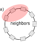
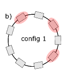
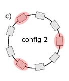
Figure 12: Example of the ways to split the whole chain formed by $N$ sites in a bipartite system formed by a subsystem $A$ and $B$ with $N_{A}$ and $N_{B}$ sites, respectively. The red region denotes the subsystem $A$. The case in a) corresponds to the partition discussed in the main text whereas the case b) and c) show configurations discussed only in this appendix.

In this appendix we report the logarithmic negativity $E_{\mathcal{N}}$ of the system for different configurations. We focus on the size $N=9$ with frustrated dissipation. Here we only deal with the coupling $\alpha=0.2$ and the ratio $\widetilde{\alpha}/\alpha=0.3$.

The logarithmic negativity $E_{\mathcal{N}}$ is an entanglement measure defined for bipartite systems. To quantify the entanglement in our single chain, we have to divide it in two parts and consider the whole chain as formed by two subsystems $A$ and $B$. A priori, there are many possible choices for a such division. Few examples of different configurations are reported in Fig. 12. In the first partition Fig. 12(a), discussed in the main text, the two subsystem are formed by neighboring islands. In the other two examples, Figs. 12(b) and 12(c), the internal sites forming the subsystem $A$ are equally spaced by one or two sites of the subsystem $B$, respectively.

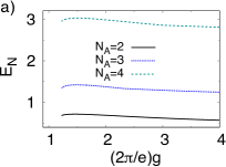
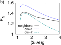
Figure 13: Logarithmic negativity for a system with $N=9$ as a function of $g$. a) The partition is fixed and corresponds to Fig. 12(a) whereas the subsystem has different size $N_{A}=2,3,4$. b) The size of they subsystem is fixed $N_{A}=3$ whereas the different configurations are reported as discussed in Fig. 12.

At a fixed configuration, corresponding to the one of Fig. 12(a), we show the result for various partition sizes ($N_{A},N-N_{A}$) with $N_{A}=2,3,4$ in Fig. 13(a). The logarithmic negativity grows with $N_{A}$ and the non-monotonic behavior is more pronounced in the latter case. In Fig. 13(b), we fix the size of the subsystem to $N_{A}=3$ and we show the results for the different partitions of the chain.

We conclude that, even if the specific slope depends on the configuration and size of the subsystem, the non-monotonic behavior still appears as a characteristic feature in the system affected by dissipative frustration.

References

- Buluta and Nori (2009) I. Buluta and F. Nori, Science 326, 108 (2009).
- Cirac and Zoller (2012) J. I. Cirac and P. Zoller, Nature Physics 8, 264 (2012).
- Georgescu et al. (2014) I. M. Georgescu, S. Ashhab, and F. Nori, Review Modern Physics 86, 153 (2014).
- Greiner et al. (2002) M. Greiner, O. Mandel, T. Esslinger, T. W. Hänsch, and I. Bloch, Nature 415, 39 (2002).
- Bloch et al. (2012) I. Bloch, J. Dalibard, and S. Nascimbène, Nature Physics 8, 267 (2012).
- Barreiro et al. (2011) J. T. Barreiro, M. Müller, P. Schindler, D. Nigg, T. Monz, M. Chwalla, M. Hennrich, C. F. Roos, P. Zoller, and R. Blatt, Nature 470, 486 (2011).
- Blatt and Roos (2012) R. Blatt and C. F. Roos, Nature Physics 8, 277 (2012).
- Kim and Yamamoto (2017) N. Y. Kim and Y. Yamamoto, in Quantum Simulations with Photons and Polaritons: Merging Quantum Optics with Condensed Matter Physics, edited by D. G. Angelakis (Springer International Publishing, Cham, 2017) pp. 91–121.
- Leib and Hartmann (2010) M. Leib and M. J. Hartmann, New Journal of Physics 12, 093031 (2010).
- Hartmann (2016) M. J. Hartmann, Journal of Optics 18, 104005 (2016).
- Salathé et al. (2015) Y. Salathé, M. Mondal, M. Oppliger, J. Heinsoo, P. Kurpiers, A. Potočnik, A. Mezzacapo, U. Las Heras, L. Lamata, E. Solano, S. Filipp, and A. Wallraff, Physical Review X 5, 021027 (2015).
- Barends et al. (2015) R. Barends, L. Lamata, J. Kelly, L. García-Álvarez, A. G. Fowler, A. Megrant, E. Jeffrey, T. C. White, D. Sank, J. Y. Mutus, B. Campbell, Y. Chen, Z. Chen, B. Chiaro, A. Dunsworth, I. C. Hoi, C. Neill, P. J. J. O’Malley, C. Quintana, P. Roushan, A. Vainsencher, J. Wenner, E. Solano, and J. M. Martinis, Nature Communications 6, 8654 (2015).
- Makhlin et al. (2001) Y. Makhlin, G. Schön, and A. Shnirman, Review Modern Physics 73, 357 (2001).
- Zagoskin (2011) A. M. Zagoskin, Quantum Engineering - Theory and Design of Quantum Coherent Structures (Cambridge University Press, Cambridge, 2011).
- Li et al. (2014) Z. Li, H. Zhou, C. Ju, H. Chen, W. Zheng, D. Lu, X. Rong, C. Duan, X. Peng, and J. Du, Physical Review Letters 112, 220501 (2014).
- Biella et al. (2015) A. Biella, L. Mazza, I. Carusotto, D. Rossini, and R. Fazio, Physical Review A 91, 053815 (2015).
- Zippilli et al. (2015) S. Zippilli, J. Li, and D. Vitali, Physical Review A 92, 032319 (2015).
- Hacohen-Gourgy et al. (2015) S. Hacohen-Gourgy, V. V. Ramasesh, C. De Grandi, I. Siddiqi, and S. M. Girvin, Physical Review Letters 115, 240501 (2015).
- Labouvie et al. (2016) R. Labouvie, B. Santra, S. Heun, and H. Ott, Physical Review Letters 116, 235302 (2016).
- Wolff et al. (2016) S. Wolff, A. Sheikhan, and C. Kollath, Physical Review A 94, 043609 (2016).
- Fitzpatrick et al. (2017) M. Fitzpatrick, N. M. Sundaresan, A. C. Y. Li, J. Koch, and A. A. Houck, Physical Review X 7, 011016 (2017).
- Fernández-Lorenzo and Porras (2017) S. Fernández-Lorenzo and D. Porras, Physical Review A 96, 013817 (2017).
- Banchi et al. (2017) L. Banchi, J. Fernández-Rossier, C. F. Hirjibehedin, and S. Bose, Physical Review Letters 118, 147203 (2017).
- Raghunandan et al. (2018) M. Raghunandan, J. Wrachtrup, and H. Weimer, Phys. Rev. Lett. 120, 150501 (2018).
- Foss-Feig et al. (2017) M. Foss-Feig, J. T. Young, V. V. Albert, A. V. Gorshkov, and M. F. Maghrebi, Physical Review Letter 119, 190402 (2017).
- Fazio and van der Zant (2001) R. Fazio and H. van der Zant, Physics Reports 355, 235 (2001).
- Wood and Stroud (1982) D. M. Wood and D. Stroud, Physical Review B 25, 1600 (1982).
- Bradley and Doniach (1984) R. M. Bradley and S. Doniach, Physical Review B 30, 1138 (1984).
- Jacobs et al. (1984) L. Jacobs, J. V. José, and M. A. Novotny, Physical Review Letters 53, 2177 (1984).
- Devillard (2011) P. Devillard, Physical Review B 83, 094509 (2011).
- Sachdev (2007) S. Sachdev, Quantum phase transitions (Wiley Online Library, 2007).
- Sondhi et al. (1997) S. L. Sondhi, S. M. Girvin, J. P. Carini, and D. Shahar, Review Modern Physics 69, 315 (1997).
- Chow et al. (1998) E. Chow, P. Delsing, and D. B. Haviland, Physical Review Letters 81, 204 (1998).
- Kuo and Chen (2001) W. Kuo and C. D. Chen, Physical Review Letters 87, 186804 (2001).
- Fisher et al. (1989) M. P. A. Fisher, P. B. Weichman, G. Grinstein, and D. S. Fisher, Physical Review B 40, 546 (1989).
- Bruder et al. (1993) C. Bruder, R. Fazio, and G. Schön, Physical Review B 47, 342 (1993).
- Roddick and Stroud (1993) E. Roddick and D. Stroud, Physical Review B 48, 16600 (1993).
- van Otterlo et al. (1995) A. van Otterlo, K.-H. Wagenblast, R. Baltin, C. Bruder, R. Fazio, and G. Schön, Physical Review B 52, 16176 (1995).
- Freericks and Monien (1996) J. K. Freericks and H. Monien, Physical Review B 53, 2691 (1996).
- Odintsov (1996) A. A. Odintsov, Physical Review B 54, 1228 (1996).
- Glazman and Larkin (1997) L. I. Glazman and A. I. Larkin, Physical Review Letters 79, 3736 (1997).
- Sarkar (2007) S. Sarkar, Physical Review B 75, 014528 (2007).
- Bard et al. (2017) M. Bard, I. V. Protopopov, I. V. Gornyi, A. Shnirman, and A. D. Mirlin, Physical Review B 96, 064514 (2017).
- Cedergren et al. (2017) K. Cedergren, R. Ackroyd, S. Kafanov, N. Vogt, A. Shnirman, and T. Duty, Physical Review Letters 119, 167701 (2017).
- Yoshino et al. (2010) H. Yoshino, T. Nogawa, and B. Kim, Progress of Theoretical Physics Supplement 184, 153 (2010).
- Meier et al. (2015) H. Meier, R. T. Brierley, A. Kou, S. M. Girvin, and L. I. Glazman, Physical Review B 92, 064516 (2015).
- Panyukov and Zaikin (1987) S. Panyukov and A. Zaikin, Physics Letters A 124, 325 (1987).
- Korshunov (1989) S. E. Korshunov, Europhysics Letters 9, 107 (1989).
- Bobbert et al. (1990) P. A. Bobbert, R. Fazio, G. Schön, and G. T. Zimanyi, Physical Review B 41, 4009 (1990).
- Bobbert et al. (1992) P. A. Bobbert, R. Fazio, G. Schön, and A. D. Zaikin, Physical Review B 45, 2294 (1992).
- Chakravarty et al. (1986) S. Chakravarty, G.-L. Ingold, S. Kivelson, and A. Luther, Physical Review Letters 56, 2303 (1986).
- Fisher (1987) M. P. A. Fisher, Physical Review B 36, 1917 (1987).
- Chakravarty et al. (1988) S. Chakravarty, G.-L. Ingold, S. Kivelson, and G. Zimanyi, Physical Review B 37, 3283 (1988).
- Zwerger (1989) W. Zwerger, Europhysics Letters 9, 421 (1989).
- Wagenblast et al. (1997) K.-H. Wagenblast, A. van Otterlo, G. Schön, and G. T. Zimányi, Phys. Rev. Lett. 79, 2730 (1997).
- Refael et al. (2007) G. Refael, E. Demler, Y. Oreg, and D. S. Fisher, Physical Review B 75, 014522 (2007).
- Miyazaki et al. (2002) H. Miyazaki, Y. Takahide, A. Kanda, and Y. Ootuka, Physical Review Letters 89, 197001 (2002).
- Lobos and Giamarchi (2011) A. M. Lobos and T. Giamarchi, Physical Review B 84, 024523 (2011).
- Kohler and Sols (2005) H. Kohler and F. Sols, Physical Review B 72, 180404 (2005).
- Kohler and Sols (2006) H. Kohler and F. Sols, New Journal of Physics 8, 149 (2006).
- Cuccoli et al. (2010) A. Cuccoli, N. Del Sette, and R. Vaia, Physical Review E 81, 041110 (2010).
- Kohler and Sols (2013) H. Kohler and F. Sols, Physica A: Statistical Mechanics and its Applications 392, 1989 (2013).
- Rastelli (2016) G. Rastelli, New Journal of Physics 18, 053033 (2016).
- Castro Neto et al. (2003) A. H. Castro Neto, E. Novais, L. Borda, G. Zarand, and I. Affleck, Physical Review Letters 91, 096401 (2003).
- Novais et al. (2005) E. Novais, A. H. Castro Neto, L. Borda, I. Affleck, and G. Zarand, Physical Review B 72, 014417 (2005).
- Kohler et al. (2013) H. Kohler, A. Hackl, and S. Kehrein, Physical Review B 88, 205122 (2013).
- Bruognolo et al. (2014) B. Bruognolo, A. Weichselbaum, C. Guo, J. von Delft, I. Schneider, and M. Vojta, Physical Review B 90, 245130 (2014).
- Zhou et al. (2015) N. Zhou, L. Chen, D. Xu, V. Chernyak, and Y. Zhao, Physical Review B 91, 195129 (2015).
- Giuliano and Sodano (2008) D. Giuliano and P. Sodano, New Journal of Physics 10, 093023 (2008).
- Lang and Büchler (2015) N. Lang and H. P. Büchler, Physical Review A 92, 012128 (2015).
- Kugler (1969) A. A. Kugler, Annals of Physics 53, 133 (1969).
- Gillis and Koehler (1972) N. S. Gillis and T. R. Koehler, Physical Review Letters 29, 369 (1972).
- Moleko and Glyde (1983) L. K. Moleko and H. R. Glyde, Physical Review B 27, 6019 (1983).
- Kampf and Schön (1987) A. Kampf and G. Schön, Physical Review B 36, 3651 (1987).
- Samathiyakanit and Glyde (1973) V. Samathiyakanit and H. R. Glyde, Journal of Physics C: Solid State Physics 6, 1166 (1973).
- Rastelli and Ciuchi (2005) G. Rastelli and S. Ciuchi, Physical Review B 71, 184303 (2005).
- Rastelli and Cappelluti (2011) G. Rastelli and E. Cappelluti, Physical Review B 84, 184305 (2011).
- Polak and KopeÄ (2007) T. Polak and T. KopeÄ, Physica C: Superconductivity and its Applications 455, 25 (2007).
- Polak and Kopeć (2005) T. P. Polak and T. K. Kopeć, Phys. Rev. B 72, 014509 (2005).
- Feynman et al. (2010) R. P. Feynman, A. R. Hibbs, and D. F. Styer, Quantum mechanics and path integrals (Courier Corporation, 2010).
- Kleinert (2009) H. Kleinert, Path Integrals in Quantum Mechanics, Statistics, Polymer Physics, and Financial Markets - (World Scientific, Singapur, 2009).
- Weiss (2012) U. Weiss, Quantum Dissipative Systems - (World Scientific, Singapur, 2012).
- Tinkham (1996) M. Tinkham, Introduction to Superconductivity, 2nd ed. (McGraw-Hill, New York, 1996).
- (84) Note that, in absence of the dissipative coupling, the phase is a compact variable and the integration includes over all possible paths with boundary conditions ( integer) Kleinert (2009). When the phase is coupled to an external bath, we have the decompactification, see discussion in Refs. Fazio and van der Zant (2001); Apenko (1989). In any cases, within the SCHA, this distinction is no relevant since we assume strongly localized phases and neglect phase slips events, i.e. fluctuations of the order of .
- Apenko (1989) S. M. Apenko, Physical Letters A 4,5, 277 (1989).
- Note (1) Notice that, if we set , we have , in which we can use (or and ). With this we can find the relations and , where the subscripts and stand for the and the part of the Fourier transformation, respectively.
- Note (2) Note that this value differs from the one found by Chakravarty et. al. Chakravarty et al. (1988), because they used the further approximation that the dispersion of the modes was purely linear.
- Nielsen and Chuang (2010) M. Nielsen and I. Chuang, Quantum Computation and Quantum Information (10th Anniversary Edition) (Cambridge University Press, 2010).
- Adesso and Illuminati (2007) G. Adesso and F. Illuminati, Journal of Physics A: Mathematical and Theoretical 40, 7821 (2007).
- Vidal and Werner (2002) G. Vidal and R. F. Werner, Physical Review A 65, 032314 (2002).
- Wolf et al. (2006) M. M. Wolf, G. Giedke, and J. I. Cirac, Phys. Rev. Lett. 96, 080502 (2006).
- Peres (1996) A. Peres, Physical Review Letters 77, 1413 (1996).
- Horodecki et al. (1996) M. Horodecki, P. Horodecki, and R. Horodecki, Physics Letters A 223, 1 (1996).
- Note (3) Since is still Hermitian with then we have .
- Patanè et al. (2007) D. Patanè, R. Fazio, and L. Amico, New Journal of Physics 9, 322 (2007).
- Simon (2000) R. Simon, Physical Review Letters 84, 2726 (2000).
- Serafini (2006) A. Serafini, Physical Review Letters 96, 110402 (2006).
- Devoret (2002) M. H. Devoret, in Quantum Fluctuations (Les Houches Session LXIII) (Elsevier, Amsterdam, 2002) p. 1.