Fitting and selecting scattering data

Abstract:

The main purpose of scattering experiments is to unveil the underlying structure of the colliding particles and their interaction. Typically one measures scattering observables (cross sections and polarizations) at discrete angles and energies and mutually consistent data may validate or falsify proposed theories or models. However, the accumulation of data from different laboratories while potentially improves the statistical significance it may sometimes generate mutually inconsistent data as a side-effect. Thus, some decision has to be made on what are the maximal amount of data which are mutually compatible. We show elastic $\pi N$ and $NN$ scattering as prominent examples where this selection is called for. We discuss how it can be done in a self-consistent manner invoking a principle of maximal consensus of the database and with the help of a sufficiently flexible model involving a minimal number of theoretical assumptions. In the NN case this has become possible with a combination of long distance field theoretical constraints at the hadronic level such as pion exchanges and electromagnetic effects and a coarse graining of the unknown interaction over the shortest de Broglie wavelength being probed in the scattering process.

1 Introduction

Fitting and selecting scattering data are intertwined activities with a long tradition in Nuclear and Particle Physics. In the absence of mutually inconsistent data, theories may be validated or falsified by data, since only in such a case a satisfactory fit becomes possible. Thus, ensuring that this is indeed the case allows one to answer important questions. We stress from the beginning that the issues which we will be discussing were proposed many years ago . In this contribution we revisit the subject at a comprehensive level as we feel that essential issues are too often forgotten. More details and references within the NN context can be traced from [7, 8, 9, 10, 11, 12, 13, 14].

2 Scattering

Scattering experiments are designed after the original Rutherford experiment which lead to the discovery of the atomic nucleus in 1908: $N_{\rm in}$ particles emitted from a source of surface $S$ are collimated forming a beam which is scattered at a given solid angle $\Omega\equiv(\theta,\phi)$ and $N_{\rm out}$ particles are counted on a detector at a far distance $R$. The differential cross section is defined as the ratio

$$\sigma_{\rm exp}(\theta,\phi)=\frac{N_{\rm out}(\theta,\phi)/\Delta\Omega}{N_{\rm in}/S}\,,$$ (1)

over a given time interval and detector angular resolution $\Delta\Omega=(\Delta\theta,\Delta\phi)$. In general, there exists a normalization constant, which can be determined by comparing with a theoretically known cross section or by checking the total cross section $\sigma_{T}\equiv\int d\Omega\sigma(\Omega)$ with a forward transmission experiment where the mean free path is determined $l=1/n\sigma_{T}$ and the density of scatterers per unit volume, $n$, is known. We assume for simplicity non-relativistic elastic scattering for spinless particles interacting by a central potential $V(r)$.

At the classical level, one solves Newton’s equation $\mu{\vec{x}}^{\prime\prime}(t)=-\vec{\nabla}V(\vec{x})$ subjected to the conditions $\vec{x}(t)\to\vec{b}+\vec{v}t$ and $\vec{x}(t)\to\vec{b}^{\prime}+\vec{v}^{\prime}t$ for $t\to\mp\infty$ respectively, where $\vec{b}\cdot\vec{v}=b^{\prime}\cdot\vec{v}^{\prime}=0$, $\hat{v}^{\prime}\cdot\hat{v}=\hat{b}^{\prime}\cdot\hat{b}=\cos\theta$ and $\sigma_{\rm cl}(\theta,\phi)=d^{2}b/d\Omega=(b/\sin\theta)(db/d\theta)$. Angular momentum conservation implies $|\vec{L}(t)|=|\vec{x}(t)\wedge\vec{p}(t)|=bp=b\mu v$ and for a finite range interaction, i.e. $V(r)=0$ for $r>a$, so that $\sigma_{\rm cl}(\theta,\phi)=0$ for $b>a$. The meson exchange picture yields Yukawa-like forces among hadrons $V(r)\sim e^{-(r/a)}/r$ with the longest range corresponding to $a\sim\hbar/m_{\pi}c\sim 1.4{\rm fm}$. For these forces the total classical cross section diverges, $\sigma_{T}\equiv\int d\Omega\sigma_{\rm cl}(\Omega)=\int d^{2}b=\infty$.

Quantum mechanically one has $\sigma_{\rm QM}(\theta,\phi)=|f(\theta,\phi)|^{2}$ where the scattering amplitude reads

$$f(\theta,\phi)=\sum_{l=0}^{\infty}(2l+1)\frac{e^{2i\delta_{l}(p)}-1}{2ip}P_{l}(\cos\theta)\quad,\qquad E=\frac{p^{2}}{2\mu}\,.$$ (2)

Here, $P_{l}(z)$ are Legendre polynomials and $\delta_{l}(p)$ are the phase-shifts which are computed by solving the reduced Schrödinger equation for the reduced wave function $u_{l}(r)$ ($\Psi(\vec{x})=(u_{l}(r)/r)Y_{l,m}(\theta,\phi)$),

$$-u_{l}^{\prime\prime}(r)+\left[\frac{l(l+1)}{r^{2}}+2\mu V(r)\right]u_{l}(r)=p^{2}u_{l}(r)$$ (3)

with the asymptotic conditions (we assume non-singular potentials $r^{2}V(r)\to 0$)

$$u_{l}(r)\underbrace{\to}_{r\to 0}r^{l+1}\quad,\qquad u_{l}(r)\underbrace{\to}_{r\to\infty}\sin\left(pr-\frac{l\pi}{2}+\delta_{l}\right)$$ (4)

The no-scattering condition corresponds to take $L^{2}=l(l+1)^{2}\sim(l+1/2)^{2}$ so that $V(r)\sim 0$ for $r\gtrsim a$ corresponds to $\delta_{l}(p)\sim 0$ for $b\gtrsim a$ or equivalently $l_{\rm max}+\frac{1}{2}\sim pa\sim p/m_{\pi}$. In this case the total cross section is now convergent for Yukawa forces. The (truncated) partial wave analysis (PWA), describes scattering data in terms of phase-shifts and known angular dependence of $P_{l}(\cos\theta)$.

Figure 1: Binomial (Histogram), Poisson (Points) and Gauss (Line) distributions for $p=0.1$ and $N=50$.

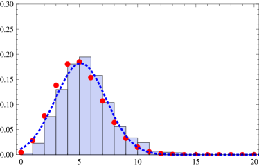
In general, the number of counts $N_{\rm out}$ is a random variable subjected to fluctuations. If for a fixed solid angle $(\theta,\phi)$ we denote by $p$ the scattering probability, the statistics of counting $k$ events out of $N$ is given by the binomial distribution with mean $\bar{k}$ and variance $(\Delta k)^{2}$,

$$P_{N,k} = \left(\begin{array}[]{c}N\\ k\end{array}\right)p^{k}(1-p)^{N-k}\,,\quad\bar{k}=Np\,,\quad(\Delta k)^{2}=\overline{(k-\overline{k})^{2}}=\overline{k^{2}}-\overline{k}^{2}=Np(1-p)\,.$$ (7)

In practice, $p\ll 1\ll k\ll N$ one has the sequence of Binomial $\to$ Poisson $\to$ Gauss distributions

$$P_{N,k} \underbrace{\to}_{p\ll 1}\frac{e^{-Np}(Np)^{k}}{k!}\underbrace{\to}_{k\gg 1}\frac{e^{-(k-Np)^{2}/2}}{\sqrt{2\pi}\Delta k}\,,$$ (8)

where in Fig. 1 we illustrate the situation for the case $p=0.1$ and $N=50$. Thus, we may consider that $N_{\rm out}$ (and hence $\sigma(\theta,E)$) is Gauss distributed. For a $68\%$ confidence level we write as usual 

$$N_{\rm out}=\bar{N}_{\rm out}\pm\Delta N_{\rm out}\,,\qquad\Delta N_{\rm out}=\sqrt{\bar{N}_{\rm out}}\,,$$ (9)

3 Fitting

Statistics. The general fitting problem corresponds to a situation where we have $N$ data with uncertainties $O_{i}\pm\Delta O_{i}$ and a theory depending on $M$-parameters ${\bf p}=(p_{1},\dots,p_{M})$ predicting $O_{i}({\bf p})$. The question: Does theory explain data ? can be answered statistically as follows. If all uncertainties follow an independent Gaussian distribution for a choice of parameters ${\bf p}$ we write

$$O_{i}^{\rm exp}=O_{i}^{\rm th}+\xi_{i}\Delta O_{i}\,,\qquad\xi_{i}\in N(0,1)\,,$$ (10)

we define the minimized least squares sum

$$\chi_{\rm min}^{2}\equiv{\rm min}_{\bf p}\chi^{2}({\bf p})=\chi^{2}({\bf p}_{0})\,,\quad\chi^{2}({\bf p})=\sum_{i=1}^{N}\left[\frac{O_{i}({\bf p})-O_{i}^{\rm exp}}{\Delta O_{i}}\right]^{2}\,.$$ (11)

This condition effectively eliminates $M$ independent variables, so that for the remaining degrees of freedom $\nu=N-M$ one has the following $\chi^{2}$ probability density distribution

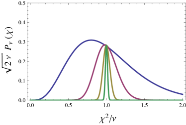
$$P_{\nu}(\chi^{2})=\prod_{n=1}^{\nu}\left(\int_{-\infty}^{\infty}d\xi_{i}\frac{e^{-\xi_{i}^{2}/2}}{\sqrt{2\pi}}\right)\delta(\chi^{2}-\sum_{n=1}^{\nu}\xi_{n}^{2})=\frac{e^{-\chi^{2}}\chi^{\nu-2}}{2^{\nu/2}\Gamma\left(\frac{\nu}{2}\right)}\,,$$ (12)

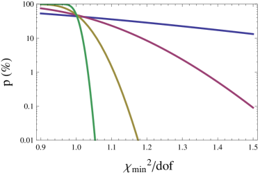
which is plotted in Fig. 2 as a function of $\chi^{2}/\nu$, and shows the drastic narrowness for a large number of data. The mean and variance are given by $\langle\chi^{2}\rangle=\nu$, $\langle(\chi^{2}-\langle\chi^{2}\rangle)^{2}\rangle=2\nu^{2}$. For $\nu\gg 1$ the $\chi^{2}\in N(\nu,\sqrt{2\nu})$ whence $\chi^{2}=\nu\pm\sqrt{2\nu}$ at the $68\%$ confidence level. Thus, the assumption that data differ from theory by fluctuations, Eq. (10), holds at $N_{\sigma}$-standard deviations level if

$$\frac{\chi_{\rm min}^{2}}{\nu}=1\pm N_{\sigma}\sqrt{\frac{2}{\nu}}\,,\quad\nu=N-M\,\quad,{\rm d.o.f\,\,(degrees\,of\,freedom)}\,.$$ (13)

Table 1 provides the case $N_{\sigma}=1$. Thus, $\chi_{\rm min}^{2}/\nu$ outside the confidence interval is unlikely (for $N_{\sigma}=1,2,3$ is less than $32,5,1\%$ respectively) and implies either a bad model or bad data or both. On the contrary, an acceptable $\chi^{2}/\nu$ suggests consistency between model and data and, more importantly, errors on the parameters reflect statistical uncertainties of the input data ${\bf p}={\bf p}_{0}+\Delta{\bf p}$ which can be propagated to functions of the parameters $F({\bf p})$ not involved in the fitting procedure.

Figure 2: The $\chi^{2}$ distribution for $\nu=10$ (blue),100 (pink),1000 (brown),10000 (green). Left panel: $\sqrt{2\nu}P_{\nu}(\chi)$ as a function of $\chi^{2}/\nu$. Right panel: $p$-value defined as $p=100\times\int_{\chi_{\rm min}^{2}}^{\infty}P_{\nu}(\chi)d\chi$.

$\nu$	10	100	1000	10000
$\chi^{2}/\nu\,$ ($68\%$)	$1\pm 0.447$	$1\pm 0.141$	$1\pm 0.044$	$1\pm 0.014.$

Table 1: Values of acceptable fits for some sample sizes at the $1\sigma$-level.

Single energy fits. The simplest situation corresponds to have complete data in a given energy $E$ (or momentum $p$), namely $\left(\sigma(\theta_{1},E),\dots,\sigma(\theta_{N},E)\right)$. In this case one can determine the $l_{\rm max}\sim pa$ phase-shifts directly from the data as fitting parameters $(\delta_{0}(E),\dots,\delta_{l_{\rm max}}(E))$ by minimizing

$$\chi^{2}(\delta_{1}(E),\dots,\delta_{l_{\rm max}}(E),Z)=\sum_{i=1}^{N}\left[\frac{\sigma^{\rm exp}(\theta_{i},E)-Z\sigma^{\rm th}(\theta_{i},\delta_{1}(E),\dots,\delta_{l_{\rm max}}(E))}{\Delta\sigma(\theta_{i},E)}\right]^{2}+\left(\frac{1-Z}{\Delta Z}\right)^{2}$$ (14)

Here the normalization $Z$ with estimated uncertainty $\Delta Z$ (provided by experimentalists) is common for one energy. Phase-shifts become “experimental” and model independent observables, $\delta_{l}^{\rm exp}(E)\pm\Delta\delta_{l}^{\rm exp}(E)$ for $l=0,\dots,l_{\rm max}$.

Multiple energy fits. If one has incomplete data in energies and angles $(\sigma(\theta_{1},E_{1}),\dots,\sigma(\theta_{N},E_{N}))$ one cannot generally determine phase-shifts $\delta_{l}(E_{i})$ at those energies. Instead, a model dependent interpolation with fitting parameters ${\bf p}$ in the energy is needed. Thus, one minimizes

$$\chi^{2}({\bf p},Z)=\sum_{i=1}^{N}\left[\frac{\sigma(\theta_{i},E_{i})^{\rm exp}-Z\sigma^{\rm th}(\theta_{i},E_{i},{\bf p})}{\Delta\sigma(\theta_{i},E_{i})}\right]^{2}+\left(\frac{1-Z}{\Delta Z}\right)^{2}$$ (15)

Different experiments have different normalizations so that generally

$$\chi^{2}({\bf p},Z_{1},\dots Z_{E})=\sum_{i=1}^{E}\chi_{i}^{2}({\bf p},Z_{i})$$ (16)

Coarse graining. In the present situation a multienergy fit becomes mandatory and the question is how to choose the fitting parameters ${\bf p}$. Our approach is based in separating the potential into a field theoretical piece and a unknown coarse grained piece at points $r_{n}$ suitably located

$$V(r)=\left[\sum_{n}\Delta rV(r_{i})\delta(r-r_{n})\right]\theta(r_{c}-r)+V_{\rm QFT}(r)\theta(r-r_{c})\quad,\qquad r_{n}=n\Delta r$$ (17)

with $\Delta r\sim 1/p_{\rm max}$ the shortest de Broglie wavelength and $r_{c}$ provides a boundary which should be larger than the elementarity size of the hadrons $r_{e}$ and turns out to be $r_{c}=1.8-3{\rm fm}$. This allows to determine a priori the number of fitting parameters, $V(r_{i})$, to be $N\sim(pr_{c})^{2}$, which are determined with errors $\pm\Delta V(r_{i})$ and turn out to be mostly uncorrelated for NN in different partial waves [8].

4 Selecting data

Figure 3: Evolution of the standard deviation $N_{\sigma}$ defined by Eq. (13) as a function of the number of data in 5 years steps for $\pi N$ at $T_{\rm LAB}^{\pi}\leq 200{\rm MeV}$ in the period 1965-2015 (left panel) and $NN=np+pp$ at $T_{\rm LAB}\leq 350{\rm MeV}$ in the period 1955-2015 (right panel). We use the SAID database http://gwdac.phys.gwu.edu/.

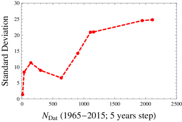
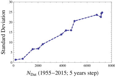
The accumulation of data improves the statistics and the precision but often generates mutually incompatible data. The need for selection becomes evident from Fig. 3 for the cases of elastic $\pi N$ and $NN$ scattering where the considered SAID fits display unlikely large $N_{\sigma}$ from Eq. (13). Taking data is painstaking and costs money. As theoreticians we do not feel qualified enough to discuss what our colleagues experimentalists do in their labs, specially since questioning one experiment means in fairness questioning all experiments. This may not necessarily mean genuinely wrong experiments, but rather unrealistic error estimates. Note that the goal of a fit is to determine the true values of certain parameters with a given and admissible confidence level. Fortunately, for a large number of experiments we can use statistics and select data according to a principle of consensus among experiments arbitrated by a fitting model. Therefore, we will assume that all published experiments are correct unless proven otherwise and look for the flexible enough theory which congregates the largest number of data with an acceptable $\chi_{\rm min}^{2}/\nu\sim 1\pm\sqrt{2/\nu}$.

For NN scattering and $T_{\rm LAB}\leq 350{\rm MeV}$ we have extended the standard $3\sigma$ criterion into a self-consistency by the following selection process (see [7] for details): 1) Fit to all data. If $\chi^{2}/\nu\lesssim 1$ you can stop. If not, proceed further. 2) Remove data sets with improbably high or low contributions to the total $\chi^{2}$ (3 $\sigma$ criterion). 3) Refit parameters for the remaining data. 4) Re-apply $3\sigma$ criterion to all data. 5) Repeat until no more data are excluded or recovered.

The effect of this selection procedure is to go from $\chi^{2}/\nu|_{\rm all}=1.41$ to $\chi^{2}/\nu|_{\rm selected}=1.04$ with a reduction in the number of data from $N_{\rm Data}=8173$ to $N_{\rm Data}=6713$. While this seems a drastic rejection, the NN Granada-2013 database is the largest one to date providing a self-consistent fit below 350 MeV. For this number of data this is not a minor improvement as can be seen from Fig. 2. When the pion-nucleon coupling constants become fitting parameters $\chi^{2}/\nu|_{\rm selected}=1.025$ [13]. Moreover, normalization factors in Eq. (16) turn out to be very close to unity [7] reducing the impact of an interlab bias [15]  an issue which will be reported elsewhere. Finally, one should keep in mind that the needed data need not be $(E,\theta)$ distributed in a way that information is most useful, precise and non-redundant, a relevant aspect for large databases. If we have many data and/or accurate data in a given region of energies and angles they will tend to dominate the fit over some other regions for which there exist less data. Therefore, there is an abundance bias.

5 Discussion and outlook

There is a natural reluctance to discard data without going into the intricacies of the experiment, particularly if they are produced by influential collaborations and possibly one should simply ask the experts. When the number of experiments is large and data have been collected over the years there is no sound reason to discard old data as if wrong, because any data will eventually become old at some point. While errors are expected to be realistic, one should keep in mind that any experiment may appear to be consistent simply because both statistical and systematic errors are taken to be “conservatively” large (but also irrelevant in the $\chi^{2}$) and inconsistent if errors are “boldly” small (and extremely influential). A decision needs some underlying model and the best one should provide an acceptable fit, congregating as many data as possible. In the present contribution we have shown that we can invoke statistics to discard scattering data according to the principle of maximal consensus. The coarse graining approach has proven to be a successful framework to select NN scattering data and hence to answer important questions [12, 13, 14]. It remains to be seen if such an approach can be extended to other hadronic systems of interest.

References

- [1] E. Fermi and N. Metropolis, Numerical solution of minimum problem, Los Alamos unclassified report LS–1492, Los Alamos National Laboratory, New Mexico, USA (1952) .
- [2] S. S. Schweber, H. A. Bethe and F. De Hoffmann, Mesons and fields, Row, Peterson, 1955.
- [3] H. L. Anderson, W. C. Davidon, M. Glicksman and U. E. Kruse, Scattering of Positive Pions by Hydrogen at 189 Mev, Phys. Rev. 100 (1955) 279–287.
- [4] H. P. Stapp, T. J. Ypsilantis and N. Metropolis, Phase shift analysis of 310-MeV proton proton scattering experiments, Phys. Rev. 105 (1957) 302–310.
- [5] J. Perring, Nucleon-nucleon phase shifts at 142 mev, Nuclear Physics 42 (1963) 306–312.
- [6] R. Arndt and M. Macgregor, Chi-squared minimization techniques, Methods in Computational Physics 6 (1966) 253.
- [7] R. Navarro Pérez, J. E. Amaro and E. Ruiz Arriola, Coarse-grained potential analysis of neutron-proton and proton-proton scattering below the pion production threshold, Phys. Rev. C88 (2013) 064002, [1310.2536].
- [8] R. Navarro Perez, J. E. Amaro and E. Ruiz Arriola, Statistical error analysis for phenomenological nucleon-nucleon potentials, Phys. Rev. C89 (2014) 064006, [1404.0314].
- [9] R. Navarro Pérez, J. E. Amaro and E. Ruiz Arriola, Error analysis of nuclear forces and effective interactions, J. Phys. G42 (2015) 034013, [1406.0625].
- [10] R. Navarro Pérez, J. E. Amaro and E. Ruiz Arriola, Low energy chiral two pion exchange potential with statistical uncertainties, Phys. Rev. C91 (2015) 054002, [1411.1212].
- [11] R. Navarro Pérez, J. E. Amaro and E. Ruiz Arriola, The low-energy structure of the nucleon-nucleon interaction: statistical versus systematic uncertainties, J. Phys. G43 (2016) 114001, [1410.8097].
- [12] E. Ruiz Arriola, J. E. Amaro and R. Navarro Pérez, The falsification of Chiral Nuclear Forces, EPJ Web Conf. 137 (2017) 09006, [1611.02607].
- [13] R. N. Pérez, J. E. Amaro and E. Ruiz Arriola, Precise Determination of Charge Dependent Pion-Nucleon-Nucleon Coupling Constants, Phys. Rev. C95 (2017) 064001, [1606.00592].
- [14] I. Ruiz Simó, J. E. Amaro, E. Ruiz Arriola and R. Navarro Pérez, Low energy peripheral scaling in Nucleon-Nucleon Scattering, 1705.06522.
- [15] G. D’Agostini, Bayesian reasoning in data analysis: A critical introduction. World Scientific, 2003.