A forward–backward random process for the spectrum of 1D Anderson operators

Abstract

We give a new expression for the law of the eigenvalues of the discrete Anderson model on the finite interval $[0,N]$, in terms of two random processes starting at both ends of the interval. Using this formula, we deduce that the tail of the eigenvectors behaves approximately like $\exp(\sigma B_{|n-k|}-\gamma\frac{|n-k|}{4})$ where $B_{s}$ is the Brownian motion and $k$ is uniformly chosen in $[0,N]$ independently of $B_{s}$. A similar result has recently been shown by B. Rifkind and B. Virag in the critical case, that is, when the random potential is multiplied by a factor $\frac{1}{\sqrt{N}}$

We are interested in the one dimensional discrete Anderson model on a finite domain $[0,N]$. This model is very classical and has been studied extensively since the 70s. See for example the monograph of Carmona Lacroix [3]. Compared to higher dimensions case, it can be considered as a solved problem. However new approaches can always shed new light on this famous system.

The usual approach to tackle this system is the transfer matrix framework. The eigenvectors of the random Schrödinger operator satisfy a recursive relation of order 2, $u_{n+2}=(V_{n+1}-\lambda)u_{n+1}-u_{n}$, which can be written in a matrix form. Using this relation, one can obtain an eigenvector everywhere on $[0,N]$ from the product of the transfer matrices applied to the boundary values. The advantage of such a formulation is that one can then use the very powerful results for random matrices product and from ergodic theory such as the Oseledets theorem.

In the historical approach of Kunz and Souillard [8] or in the proof from the book [4] a change of variables is used to deal with the conditional probability of the potential $V$ with a fixed eigenvalue $\lambda$. In this short note, we propose another calculation of this conditional probability. We define a random variable $k$ whose random law is close to the uniform law on $[0,N]$. This variable splits the interval $[0,N]$ into two part $[0,k]$ and $[k,n]$. On the left part, the matrices product is made from left to right. On the right part, the matrices product is made from right to left. And far from the cut, the laws of the matrices are very close to be independent.

The main interest of our approach is that the connection with the theorems for products of random matrices is more transparent in this setup. From this formula we can recover several known results. Relying on the positivity of the Lyapunov exponent, the formula can be used as a new proof of exponential Anderson localization of eigenvectors where the center of localization is uniformly distributed on $[0,N]$. Moreover, because it gives a explicit random law, we can go beyond the exponential decay of the eigenvectors far from the center of localization and give an explicit law for their tail.

In the first section, we detail the model and we state our result. Then we give some applications of our theorem in the second section. In particular, we write an asymptotic result similar to the result of Rifkind and Virag in [10]. In Section 3, we finally give the proof of the theorem.

Acknowledgement:

We would like to thank Mathieu Lewin for his encouragement, his interest and his relevant comments. This project has received funding from the European Research Council (ERC) under the European Union’s Horizon 2020 research and innovation program (grant agreement MDFT No 725528).

1 Model and main result

We consider the discrete one dimensional Anderson model [1] defined on $[1,N]$ through the operator

$$H^{(N)}=-\Delta^{(N)}+V_{\omega}^{(N)}.$$

Here $V_{\omega}^{(N)}$ is a random iid potential and

$$\Delta^{(N)}(x,y)=\begin{cases}1&\text{if $|x-y|=1$}\\ 0&\text{otherwise}\end{cases}$$

is the usual discrete Laplacian. Hence $H$ is just the $N\times N$ symmetric matrix

$$H^{(N)}=\begin{pmatrix}V_{1}&1\\ 1&&\ddots\\ &\ddots&\ddots&\ddots\\ &&\ddots&&1\\ &&&1&V_{N}\end{pmatrix}.$$

We make the following assumption:

(H1)

The random law of $V_{\omega}$ is absolutely continuous with respect to the Lebesgue measure.

1.1 Transfer matrices

Transfer matrices have been one of the main tool to study the 1D Anderson model. One is interested in the eigenvectors, $(Hu)_{n}=\lambda u_{n}$, which satisfy the recurrence relation

$$\forall n\in[0,N],\quad-u_{n+1}+(V_{\omega}-\lambda)u_{n}-u_{n-1}=0,$$ (1)

with $u_{-1}=u_{N+1}=0$ such that the formula is valid for $n=0$ and $n=N$. This can be written with transfer matrices

$$\begin{pmatrix}u_{n+1}\\ u_{n}\end{pmatrix}=T(v_{\omega}(n)-\lambda)\begin{pmatrix}u_{n}\\ u_{n-1}\end{pmatrix}$$

where

$$\forall x,\quad T(x)=\begin{pmatrix}x&-1\\ 1&0\end{pmatrix}.$$

We can then write the matrix product

$$M_{n}(\lambda)=\prod_{k=1}^{n}T(v_{\omega}(k)-\lambda)$$

and we have

$$\begin{pmatrix}u_{n+1}\\ u_{n}\end{pmatrix}=M_{n}(\lambda)\begin{pmatrix}1\\ 0\end{pmatrix}.$$

The parameter $\lambda$ is an eigenvalue if and only if there exist $c\in\mathbb{R}$ such that

$$M_{N}(\lambda)\begin{pmatrix}1\\ 0\end{pmatrix}=\begin{pmatrix}0\\ c\end{pmatrix},$$

the condition $u_{N+1}=0$ is then satisfied.

It will be convenient to denote the vector $\begin{pmatrix}u_{n+1}\\ u_{n}\end{pmatrix}$ as a complex number in the fashion

$$u_{n+1}+iu_{n}=z_{n}=r_{n}e^{i\phi_{n}}$$

where $r_{n}\in\mathbb{R}_{+}\text{ and }\phi_{n}\in\mathbb{R}/2\pi\mathbb{Z}$. We also introduce the lifting of $\phi_{k}$, which we denote by $\theta_{k}$. This is just a discrete version of the continuous lifting from $\mathbb{R}/2\pi\mathbb{Z}$ to $\mathbb{R}$ into the discrete case. It is defined recursively by

$$\text{ }\theta_{k}=\begin{cases}\theta_{0}=0\\ \phi_{k}\ [2\pi]&\forall k\in[0,N]\end{cases}$$

and

$$\theta_{k}-\frac{\pi}{2}\leq\theta_{k+1}<\theta_{k}+\frac{3\pi}{2}.$$

It can be seen that $\phi_{k+1}$ does not depend on $r_{k+1}$ but only on $\phi_{k}$ and $T_{\lambda}(v_{k}-\lambda)$. Therefore, for simplicity of notation, we use the same notation $T$ for the operator on $\mathbb{R}/2\pi\mathbb{Z}$: $\phi_{k+1}=T_{\lambda}(v_{k})\phi_{k}$ .

Note that it is possible to recover $r_{k}$ from $\phi_{0},\phi_{1},...,\phi_{N}$ with the formula

$$\frac{r_{k+1}}{r_{k}}=\frac{r_{k+1}}{u_{k+1}}\frac{u_{k+1}}{r_{k}}=\frac{\cos\phi_{k}}{\sin\phi_{k+1}}.$$

For this reason, in the rest of the paper we focus mostly on $(\phi_{k})_{k=0\dots N}$. We note $\mathcal{F}(\lambda)=(\phi_{k})_{k=0\dots N}$ which has been constructed from the recursive formula $\phi_{k+1}=T_{\lambda}(v_{k})\phi_{k}$ and $\phi_{0}=0$. And for $\lambda$ an eigenvalue, we note $\mathcal{P}h(\lambda)=(\phi_{k})_{k=0\dots N}$ the phase of the corresponding eigenvector. Note that it is equal to $\mathcal{F}(\lambda)$ with the condition $\phi_{N}=\frac{\pi}{2}\;[\pi]$.

1.2 Forward and backward processes

In this subsection, we define two natural random laws on the chain $X=(\phi_{k})_{k=0,..,N}$. The first one is the Markov chain starting from $\phi_{0}$ with an initial law $\mu_{f}$ defined on $\mathbb{S}^{1}$ and transition law $\phi_{k}\rightarrow\phi_{k+1}=T(v_{k})\phi_{k}$ with a random measure $\nu$ for $v_{k}$. We call it the forward process. The second one is the Markov chain starting from $\phi_{N}$ with an initial law $\mu_{b}$ and transition law $\phi_{k}\rightarrow\phi_{k-1}=T_{\lambda}^{-1}(v_{k-1})\phi_{k}$ with a random measure $\nu$ for $v_{k}$ and we call it the backward process. Then we introduce a cut in $[0,N]$, and we can define the random law product between these two processes which we call the forward–backward process.

For a proper definition we use test functions on $\mathbb{R}^{N+1}$ which are bounded and continuous.

Definition 1 (Forward and backward processes).

The probability $\mathcal{P}_{f}$ on $\mathbb{R}^{N+1}$, defined by

$$\mathcal{P}_{f}(F)=\idotsint d\mu_{f}(\phi_{0})d\nu(v_{1})\cdots d\nu(v_{n})F(X)$$

for any test function $F$, is called the forward process. Similarly, the probability $\mathcal{P}_{b}$ on $\mathbb{R}^{N+1}$ defined by

$$\mathcal{P}_{b}(F)=\idotsint d\nu(v_{1})...d\nu(v_{N})d\mu_{b}(\phi_{N})F(X)$$

for any test function $F$, is called the backward process.

Remark 2.

If we introduce $\xi_{0,n}:\phi_{0}\rightarrow\phi_{n}^{f}=\prod_{k=0}^{n-1}T(v_{k})\phi_{0}$ and if for almost surely any $v_{1},v_{2},...,v_{n}$, $\mu_{b}$ and the push measure $\xi(\mu_{f})$ are equivalent measures, then we remark that for any $F$:

$\begin{aligned} \mathcal{P}_{b}(F)&=\idotsint d\nu(v_{1})...d\nu(v_{n})d\mu_{f}(X_{0})\frac{d\mu_{b}(X_{n})}{d\xi(\mu_{f}(X_{0}))}\big{|}_{v_{1},...,v_{n}}F(X)\\ &=\mathcal{P}_{f}\Bigg{(}F\frac{d\mu_{b}(X_{n})}{d\xi(\mu_{f}(X_{0}))}\big{|}_{v_{1},...,v_{n}}\Bigg{)}.\end{aligned}$

Definition 3 (Forward-Backward process).

For $k\in[0,N]$, we define $\mathcal{P}_{f,0..k}\otimes\mathcal{P}_{b,k+1,...,N}$ a forward process for $X^{f}=\phi_{0}^{f},\phi_{1}^{f}...,\phi_{k}^{f}$ with $\phi_{0}^{f}=0$, ($\mu_{f}=\delta_{0}$) and a backward process for $X^{b}=\phi_{N}^{b},\phi_{N-1}^{b}...,\phi_{k}^{b}$, with $\phi_{N}^{b}=\frac{\pi}{2}$ ($\mu_{b}=\delta_{\frac{\pi}{2}}$) which are independent from each other.

1.3 Main result

We are now ready to state the main theorem of our paper.

Theorem 4 (Law of the spectrum of the 1D Anderson model).

For any test function $G(\lambda,X)$, we have

$$\mathbb{E}\Big{[}\sum_{\lambda\in\sigma(H),X=\mathcal{P}h(\lambda)}G(\lambda,X)\Big{]}$$

$$\qquad=\int_{\mathbb{R}}d\lambda\sum_{k=1}^{N}\mathbb{E}_{\mathcal{P}_{f,1..k}\otimes\mathcal{P}_{b,k+1,...,N}}\Big{[}G(\lambda,X)\delta_{\phi_{k}^{f}-\phi_{k}^{b}[\pi]}\sin^{2}(\phi_{k}^{f})\Big{]}$$ (2)

that we can rewrite as

$$\mathbb{E}\Big{[}\frac{1}{N}\sum_{\lambda\in\sigma(H),X=\mathcal{P}h(\lambda)}G(\lambda,X)\Big{]}$$

$$\qquad=\int_{\mathbb{R}}\rho(\lambda)d\lambda\Bigg{(}\frac{1}{N}\sum_{k=1}^{N}\mathbb{E}_{\mathcal{P}_{f,1..k}\otimes\mathcal{P}_{b,k+1,...,N}}\Big{[}G(\lambda,X)\frac{\delta_{\phi_{k}^{f}-\phi_{k}^{b}[\pi]}\sin^{2}(\phi_{k}^{f})}{\rho(\lambda)}\Big{]}\Bigg{)}$$ (3)

with $\rho(\lambda)$ the density of state.

Recall that $Ph(\lambda)$ is the phase of the eigenvector corresponding to the eigenvalue $\lambda$.

This formula is to be understood as follows. One chooses $k$ randomly in $[1,N]$ which splits the segment into two parts $[1,k]$ and $[k,N]$. On the left, we obtain a forward process, on the right, we obtain a backward process. The choice of $k$ is not exactly uniform on $[0,N]$ because of the condition $\delta_{\phi_{k}^{f}-\phi_{k}^{b}}\sin^{2}(\phi_{k})$. However, for large $N$, and for any $k\leq N$ not too close to $0$ or $N$, the laws of $\phi_{k}^{f}$ and $\phi_{k}^{b}$ are very close to their invariant measure and then do not depend on $k$. Therefore the law of $k$ becomes close to the uniform.

There is still a dependence between the two processes at the connection between the forward and backward processes. However, because of the mixing property of the matrix product, the correlations decay exponentially fast away from the cut $k$.

We recall that a stationary process $X_{k}$ is called $(\alpha_{n})_{n\in\mathbb{N}}-$ mixing if

$$\forall k,\quad\max_{A,B}|\mathbb{P}(X_{k}\in A,X_{k+n}\in B)-\mathbb{P}(X_{k}\in A)\mathbb{P}(X_{k+n}\in B)|\leq\alpha_{n}$$

The following is a well known result.

Proposition 5.

There exists a constant $C>0\text{ and }0<\kappa<1$ such that the process $\phi_{k}$ is $(C\kappa^{n})_{n\in\mathbb{N}}-$mixing.

For a proof, see [3, proposition IV.3.12].

2 Applications

We present here three application of our result. The first one is a formula for the integrated density of states. The second one is about the form of the tails of the eigenvectors. We then finish with a temperature profile from [5].

2.1 A formula for the integrated density of states

The following equality can be found as well in [3] (proposition VIII.3.10 and problem VIII.6.8).

Proposition 6.

For $\lambda\in\mathbb{R}$, let $\mu_{\lambda}(d\phi)=m_{\lambda}(\phi)d\phi$ be the $T_{\lambda}$-invariant measure on $\mathbb{R}/\mathbb{Z}$. The density of states

$$dN(\lambda)=\lim_{N\rightarrow\infty}\frac{1}{N}\#\big{\{}\sigma(H)\cap[\lambda,\lambda+d\lambda]\big{\}}$$

is given by

$$\frac{dN(\lambda)}{d\lambda}=\int_{\mathbb{\mathbb{R}}/2\mathbb{\pi\mathbb{Z}}}\sin^{2}(\phi)m_{\lambda}(\phi)m_{\lambda}\Big{(}\frac{\pi}{2}-\phi\Big{)}d\phi.$$

Proof.

We apply our formula (3) in Theorem 4. We choose $G(s,X)=G(s)$ (that does not depend on $X$) and recognize $\int_{\mathbb{R}}G(\lambda)\rho(\lambda)d\lambda$. More precisely,

$$\frac{1}{N}\mathbb{E}\Big{[}\sum_{\lambda\in\sigma(H_{N})}G(\lambda)\Big{]} =\int G(\lambda)d\lambda\frac{1}{N}\sum_{k}\mathbb{E}_{\mathcal{P}_{f,1..k}\otimes\mathcal{P}_{b,k+1,...,N}}[\delta_{\phi_{k}^{f}-\phi_{k}^{b}}\sin^{2}(\phi_{k})]$$

$$=\int G(\lambda)d\lambda\frac{1}{N}\sum_{k}\int_{\phi}\rho_{k,\lambda}(\phi)\rho_{N-k,\lambda}(\frac{\pi}{2}-\phi)\sin^{2}(\phi_{k})]$$

where $\rho_{k,\lambda}$ and $\rho_{N-k,\lambda}$ are the density probabilities of the angles of $M_{k}(\lambda)\begin{pmatrix}1\\ 0\end{pmatrix}$ and $M_{N-k}(\lambda)\begin{pmatrix}1\\ 0\end{pmatrix}$. We can then conclude using that $\rho_{k,\lambda}\rightarrow m_{\lambda}$ and $\rho_{N-k,\lambda}\rightarrow m_{\lambda}$ when $k\rightarrow\infty$ and $N-k\rightarrow\infty$. ∎

2.2 Brownian and drift for the eigenvectors

It is well known since the work of Carmona-Klein-Martinelli [2], Goldsheild-Molchanov-Pastur [7] and Kunz-Souillard [8] that the eigenvectors are localized and decay exponentially from the center of localization. An exact form of the eigenvectors has been recently proven in the critical case where $V$ is replaced by $\frac{V}{\sqrt{N}}$ in [10]. The authors proved that the eigenvectors in the bulk have the form $e^{\sigma\frac{B_{|t-u|}}{2}-\gamma|t-u|}$. We claim using our formula of Theorem 4 that a similar result holds for the tails of the eigenvectors in the non critical case.

For the reader’s convenience we recall the heuristics of the following classical results. One can write any product of random matrices $M_{N}=\prod_{i=1}^{N}T_{i}$ as

$$\log(\|M_{N}\|)=\log\Big{(}\prod_{i=1}^{N}\frac{\|M_{i}\|}{\|M_{i-1}\|}\Big{)}=\sum_{i=1}^{N}\log\Big{(}\|T_{i}\big{(}\frac{M_{i-1}}{\|M_{i-1}\|}\big{)}\|\Big{)}$$

In the case when $T_{i}$ are iid and there are some strong mixing property on $\frac{M_{i-1}}{\|M_{i-1}\|}$, the terms $Y_{i}=\log\Big{(}\|T_{i}\big{(}\frac{M_{i-1}}{\|M_{i-1}\|}\big{)}\|\Big{)}$ should behave like iid random variables. One can then prove the strong law of large numbers, the central limit theorem, and Donsker’s theorem. See the paper of Le Page [9] for these results. One therefore defines a “mean”, a “variance” and a “random walk“ as follows.

Definition 7.

The Lyapunov exponent is

$$\gamma(\lambda):=\lim_{N\rightarrow\infty}\frac{1}{N}\mathbb{E}\big{[}\log\|M_{N}(\lambda)\|\big{]}.$$

The limit variance is

$$\sigma^{2}(\lambda)=\lim_{N\rightarrow\infty}\frac{1}{N}\mathbb{E}\big{[}(\log\|M_{N}(\lambda)\|-\gamma(\lambda)N)^{2}\big{]}.$$

The random walk is

$$S_{n}=\frac{1}{\sigma(\lambda)}\big{(}\log\|M_{n}(\lambda)\|-\gamma(\lambda)n\big{)}.$$

and we consider its rescaling

$$W_{N}(t)=\frac{1}{\sqrt{N}}S_{\lfloor Nt\rfloor}.$$

Finally, we denote by $W$ the Wiener measure.

Theorem 8 (Limit theorem for products of random matrices).

We have the following:

• $\gamma(\lambda)>0$ and $\lim_{N\rightarrow\infty}\frac{1}{N}\log\|M_{N}(\lambda)\|=\gamma$, almost surely;

• $\sigma^{2}(\lambda)>0$;

• $W_{N}\rightarrow W$ in law.

We refer to [9, Theorems 2 and 3] for the proof of Theorem 8.

We recover then the form of Brownian with drift and both on the right hand side and the left hand side of the cut. For $\lambda$ an eigenvalue, and $r_{k}e^{i\phi_{k}}$ the corresponding eigenvector, we note $q_{k}^{\lambda}=\log(r_{k})$. For scaling, we set $q^{\lambda}(s)=q_{\lfloor Ns\rfloor}^{\lambda}/N$.

Proposition 9 (Tail of eigenvectors).

1) Choosing $\lambda^{(N)}$ uniformly in $\sigma(H^{(N)})$, we have the following convergence in law

$$(\lambda^{(N)},q_{s}^{\lambda^{(N)}})\rightarrow_{N\infty}(\tilde{\lambda},-|\gamma(\tilde{\lambda})(s-x)|)$$

where $\tilde{\lambda}$ is a random variable with law the limiting density of state $\rho$ and $x$ an independent variable on $[0,1]$ with uniform law.

2) There exists a sequence of random variables $\{x^{(N)}\}$ with uniform law on $[0,1]$ such that

$$(\lambda^{(N)},\sqrt{N}\big{[}q_{s}^{\lambda^{(N)}}+|\gamma(\lambda^{N})(s-x^{(N)})|\big{]})\rightarrow_{N\infty}(\tilde{\lambda},\sigma(\tilde{\lambda})W_{s-x})$$

where $W$ is the Wiener measure.

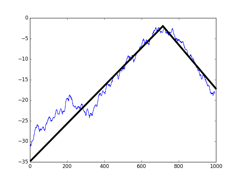
The first statement is the very classical result of Anderson localization for the one dimensional model. The eigenvectors decay exponentially from their center of localization and this center is chosen uniformly on the domain. The second statement says that the typical deviation from the decay is the exponential of a Brownian (see Figure 1 for an illustration).

Rifkind and Virag [10] studied the large eigenvectors of the one dimensional Anderson model in the continuous case where the potential is a white noise. It is the limit of the discrete model in the “critical regime” where the potential is scaled like $V_{\omega}^{(N)}=\frac{1}{\sqrt{N}}V_{\omega}$. In this regime, one cannot speak of localization because the length of the decay is as large as the size of the domain. However they proved the exact law of the form of the eigenvectors

$$q_{s}^{\lambda}=-|\gamma(\lambda)(s-x)|+\sigma(\lambda)W_{s-x}.$$

To make the connection with our previous proposition, one can actually show that for $V_{\omega}=\epsilon v_{\omega}$, with $\mathbb{E}(v_{\omega}^{2})=\sigma^{2}$, in the limit $\epsilon\rightarrow 0$ and $|\lambda|<2,$ we have

$$\gamma(\lambda)=\frac{\sigma^{2}}{4-\lambda^{2}}\epsilon^{2}$$

and

$$\frac{\sigma(\lambda)^{2}}{2}=\frac{\sigma^{2}}{4-\lambda^{2}}\epsilon^{2}.$$

Figure 1: A realization of $\log\|M_{n}(\lambda)\|$ for $N=1000$, $v_{\omega}$ uniform on $[0,1]$ with Dirichlet boundary conditions. we add a fit of the form $|\gamma(\lambda)(s-x)|$.

Proof of Proposition 9.

If in our formula (3) the term $\delta_{\phi_{k}^{f}-\phi_{k}^{b}}$ were not there, then the forward and the backward processes would be completely independent. Our proposition would have then immediately followed from Theorem 8, under the conditions that $r_{k}$ obtained by the forward process and the $r_{k}$ obtained by the backward process are the same, and that the normalization $\sum_{n=1}^{N}|u_{n}|^{2}=1$ holds. The latter becomes in the limit $\sup q_{s}^{\lambda}=0$.

Therefore we only have to check that the little perturbation around the cut $k$ has no influence. We fix $\phi$. Conditionally of $\phi_{k}^{b}=\phi$ and $\phi_{k}^{f}=\phi$ the forward and backward processes are independent. The results of Theorem 8 are true asymptotically with probability $1$. Therefore for any $\phi$ in a set of full Lebesgue measure in $\mathbb{S}^{1}$ the results of Theorem 8 are true conditionally of $\phi_{k}^{b}=\phi$ and $\phi_{k}^{f}=\phi$. ∎

2.3 A temperature profile

We will use our result to explain some numerical observations which have been made in [5]. In this article, the authors are interested in the temperature profile of a disordered chain connected to two thermal baths of temperatures $T_{0}$ and $T_{N}$ at the boundary $0$ and $N$. According to [5], the temperature $T(x)$ at site $x$ is expected to be given in a certain limit by

$$T(x)=\sum_{\lambda\in\sigma(H)}|\psi_{\lambda}(x)|^{2}\Big{(}T_{0}\frac{|\psi_{\lambda}(0)|^{2}}{|\psi_{\lambda}(0)|^{2}+|\psi_{\lambda}(N)|^{2}}+T_{N}\frac{|\psi_{\lambda}(N)|^{2}}{|\psi_{\lambda}(0)|^{2}+|\psi_{\lambda}(N)|^{2}}\Big{)}$$ (4)

where $H$ is our one–dimensional random Schrödinger operator and $\psi_{\lambda}$ are its eigenvectors.

We prove that $T$ converge to a step function where the transition from $T_{0}$ and $T_{N}$ happens in a neibourghood of $x=\frac{N}{2}$ at a scale $\sqrt{N}$. This has been observed numerically in [5].

Proposition 10.

For $N$ large enough we have

$$\lim_{N\rightarrow\infty}\mathbb{E}\big{[}T(\lfloor\sqrt{N}x+\frac{N}{2}\rfloor)\big{]}=T_{0}+(T_{N}-T_{0})\int_{\mathbb{R}}\mathbb{P}\Big{(}\mathcal{N}(0,1)\leq\frac{2\gamma(\lambda)}{\sigma(\lambda)}x\Big{)}dN(\lambda)$$

where $dN(\lambda)$ is the integrated density of states, $\gamma(\lambda)$ is the Lyapunov exponent and $\sigma(\lambda)$ is the limit variance.

The Lyapunov exponent is positive, continuous and so is bounded below on the support of $\sigma(H)$. The variance $\sigma(\lambda)$ is bounded as well. Therefore, uniformly in $\lambda$, $\mathbb{P}(\mathcal{N}(0,1)\leq\frac{\sigma(\lambda)}{2\gamma(\lambda)}x)\rightarrow 0$ for $x\rightarrow-\infty$ and $\mathbb{P}(\mathcal{N}(0,1)\leq\frac{\sigma(\lambda)}{2\gamma(\lambda)}x)\rightarrow 1$ for $x\rightarrow\infty$. We have then $T(y)=T_{0}$ for $\frac{N}{2}-y\gg\sqrt{N}$ and $T(y)=T_{N}$ for $y-\frac{N}{2}\gg\sqrt{N}$. This is the step function numerically observed in [5].

Proof.

We use our formula and write:

$$\mathbb{E}(T(x))=\sum_{k\in[0,N]}\int_{\mathbb{R}}d\lambda\mathbb{E}_{\mathcal{P}_{f,1..k}\otimes\mathcal{P}_{b,k+1,...,N}}\Big{[}|\psi_{\lambda}(x)|^{2}\\ \left(T_{0}\frac{|\psi_{\lambda}(0)|^{2}}{|\psi_{\lambda}(0)|^{2}+|\psi_{\lambda}(N)|^{2}}+T_{N}\frac{|\psi_{\lambda}(N)|^{2}}{|\psi_{\lambda}(0)|^{2}+|\psi_{\lambda}(N)|^{2}}\right)\delta_{\phi_{k}^{f}-\phi_{k}^{b}}\sin^{2}(\phi_{k})\Big{]}$$

With the notation of Proposition 9, we write

$$T_{0}\frac{|\psi_{\lambda}(0)|^{2}}{|\psi_{\lambda}(0)|^{2}+|\psi_{\lambda}(N)|^{2}}+T_{N}\frac{|\psi_{\lambda}(N)|^{2}}{|\psi_{\lambda}(0)|^{2}+|\psi_{\lambda}(N)|^{2}}\\ =T_{0}\frac{e^{Nq_{0}^{\lambda^{(N)}}}}{e^{Nq_{0}^{\lambda^{(N)}}}+e^{Nq_{1}^{\lambda^{(N)}}}}+T_{1}\frac{e^{Nq_{1}^{\lambda^{(N)}}}}{e^{Nq_{0}^{\lambda^{(N)}}}+e^{Nq_{1}^{\lambda^{(N)}}}}.$$

Therefore in the limit $N\to\infty$, this converges to $T_{0}$ for $q_{0}^{\lambda}>q_{1}^{\lambda}$ and $T_{1}$ for $q_{0}^{\lambda}<q_{1}^{\lambda}$. We have then at the limit a Bernoulli $T_{int}$ with parameter given by Proposition 9:

$$T_{int}=\begin{cases}T_{0}&\text{with probability }\mathbb{P}\left(\mathcal{N}(0,1)\leq\frac{(2k-N)\gamma(\lambda)}{\sqrt{N}\sigma(\lambda)}\right),\\ T_{N}&\text{with probability }\mathbb{P}\left(\mathcal{N}(0,1)\geq\frac{(2k-N)\gamma(\lambda)}{\sqrt{N}\sigma(\lambda)}\right).\end{cases}$$

In order to conclude, we recall that the whole mass of $|\psi_{\lambda}|^{2}$ is around a few number of sites around $k$ so

$$\mathbb{E}(T(x))=\int_{\mathbb{R}}d\lambda\sum_{k\in[x-\alpha(N),x+\alpha(N)]}\mathbb{E}_{\mathcal{P}_{f,1..k}\otimes\mathcal{P}_{b,k+1,...,N}}\Bigg{[}|\psi_{\lambda}(x)|^{2}\\ \left(T_{0}\frac{|\psi_{\lambda}(0)|^{2}}{|\psi_{\lambda}(0)|^{2}+|\psi_{\lambda}(N)|^{2}}+T_{N}\frac{|\psi_{\lambda}(N)|^{2}}{|\psi_{\lambda}(0)|^{2}+|\psi_{\lambda}(N)|^{2}}\right)\delta_{\phi_{k}^{f}-\phi_{k}^{b}}\sin^{2}(\phi_{k})\Bigg{]}\\ +O\left(e^{-\gamma(\lambda)\alpha(N)}\right),$$

where we have chosen $\alpha(N)$ such that $\sqrt{N}\gg\alpha(N)\text{$\gg$1}$. Moreover for large $N$,

$$\mathbb{P}(\mathcal{N}(0,1)\geq\frac{(2x-N)\gamma(\lambda)}{\sqrt{N}\sigma(\lambda)})=\mathbb{P}(\mathcal{N}(0,1)\geq\frac{(2k-N)\gamma(\lambda)}{\sqrt{N}\sigma(\lambda)})+o(1),$$

and we have then

$$\mathbb{E}(T(x))=\int_{\mathbb{R}}d\lambda\sum_{k\in[x-\alpha(N),x+\alpha(N)]}\mathbb{E}_{\mathcal{P}_{f,1..k}\otimes\mathcal{P}_{b,k+1,...,N}}\Bigg{[}|\psi_{\lambda}(x)|^{2}\\ \left(T_{0}+(T_{N}-T_{0})\mathbb{P}\left(\mathcal{N}(0,1)\geq\frac{(2x-N)\gamma(\lambda)}{\sqrt{N}\sigma(\lambda)}\right)\right)\delta_{\phi_{k}^{f}-\phi_{k}^{b}}\sin^{2}(\phi_{k})\Bigg{]}+o(1)$$

Finally we use the following formula, for $x$ not close to the edges

$$\sum_{k\in[0,N]}\mathbb{E}_{\mathcal{P}_{f,1..k}\otimes\mathcal{P}_{b,k+1,...,N}}[|\psi_{\lambda}(x)|^{2}\delta_{\phi_{k}^{f}-\phi_{k}^{b}}\sin^{2}(\phi_{k})]=\frac{dN(\lambda)}{d\lambda}+o(1).$$

Indeed, for any $A$ Borel set of $\mathbb{R}$,

$$\int_{\mathbb{R}}1_{A}(\lambda)\frac{dN(\lambda)}{d\lambda}d\lambda$$

$$\qquad=\lim\frac{1}{N}\mathbb{E}(Tr(1_{A}(H)))$$

$$\qquad=\frac{1}{N}\sum_{x}\mathbb{E}\Big{[}\sum_{\lambda\in A\cap\sigma(H)}|\psi_{\lambda}(x)|^{2}\Big{]}$$

$$\qquad=\int 1_{A}(\lambda)d\lambda\frac{1}{N}\sum_{x}\sum_{k\in[0,N]}\mathbb{E}_{\mathcal{P}_{f,1..k}\otimes\mathcal{P}_{b,k+1,...,N}}\Big{[}|\psi_{\lambda}(x)|^{2}\delta_{\phi_{k}^{f}-\phi_{k}^{b}}\sin^{2}(\phi_{k})\Big{]}.$$

We then note that the left term is asymptotically independent of $x$ for $x$ not close to the edges. Therefore

$$\int_{\mathbb{R}}1_{A}(\lambda)\frac{dN(\lambda)}{d\lambda}d\lambda$$

$$\qquad=\int 1_{A}(\lambda)d\lambda\sum_{k\in[0,N]}\mathbb{E}_{\mathcal{P}_{f,1..k}\otimes\mathcal{P}_{b,k+1,...,N}}[|\psi_{\lambda}(x)|^{2}\delta_{\phi_{k}^{f}-\phi_{k}^{b}}\sin^{2}(\phi_{k})]+o(1).$$

The proposition then follows, namely we have

$$\mathbb{E}(T(x))=T_{0}+\int_{\mathbb{R}}(T_{N}-T_{0})\mathbb{P}\Big{(}\mathcal{N}(0,1)\geq\frac{(2x-N)\gamma(\lambda)}{\sqrt{N}\sigma(\lambda)}\Big{)}\frac{dN(\lambda)}{d\lambda}d\lambda+o(1)$$

as we wanted. ∎

2.4 Periodic boundary conditions

We have tried to obtain a similar result for periodic boundary conditions. With the multiscale analysis tools [6], one has the exponential decay from the center of localization. But it would be also interesting to have an interpretation with forward backward process in this case.

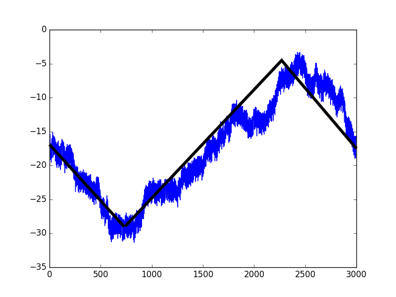
In the critical regime, one would expect the form of the eigenvectors to be like $e^{F(s)}$, on $\mathbb{R}/2\pi\mathbb{Z}$ with $F(s)=-\gamma\min(|s-u|,|s-u+\pi|)+\sigma\tilde{B}_{s-u}$ with $u$ uniformly chosen on $[0,2\pi]$ and $\tilde{B}$ a Brownian bridge. So far we have not been able to prove this statement rigorously., but our intuition seems to be confirmed by numerical simulations (see Figure 2).

Remark.

The condition $u_{-1}=u_{N+1}=0$ in the Dirichlet case has to be replaced by $\text{Tr}(M_{N}(\lambda))=2$. Indeed, let $u_{n}$ be an eigenvector of eigenvalue $\lambda$ and $z=\begin{pmatrix}u_{1}\\ u_{0}\end{pmatrix}$. Then, periodic boundary conditions mean $M_{N}(\lambda)z=z$. So $1$ is an eigenvalue of $M_{N}(\lambda)$. Therefore $1$ is a solution of $x^{2}-Tr(M_{N}(\lambda))x+1=0$ and so $\text{Tr}(M_{N}(\lambda))=2$.

Figure 2: A realization of $\log\|M_{n}(\lambda)\|$ with periodic boundary conditions for $N=3000$, $v_{\omega}$ uniform on $[0,0.3]$. We add a fit of the form $-\gamma\min(|s-u|,|s-u+\pi|)$.

3 Proof of Theorem 4

Proof.

We have that $\lambda$ is an eigenvalue if and only if $\phi_{N}=\frac{\pi}{2}[\pi]$, therefore

$$\mathbb{E}\Big{[}\sum_{\lambda\in\sigma(H),X=\mathcal{P}h(\lambda)}G(\lambda,X)\Big{]}=\mathbb{E}\Big{[}\sum_{\lambda:\theta_{N}(\lambda)\in\frac{\pi}{2}+\pi\mathbb{Z},\text{ }X=\mathcal{F}(\lambda)}G(\lambda,X)\Big{]}.$$

Remark 11.

$\theta_{N}:\lambda\rightarrow\theta_{N}(\lambda)$ is continuous and strictly increasing (see the calculations below).

For finite $N$, the inverse function $\theta_{N}^{-1}$ is continuous, so are $G$, $X$. We can therefore write

$$\mathbb{E}\Big{[}\sum_{\lambda:\theta_{N}(\lambda)\in 2\pi\mathbb{Z},X=\mathcal{F}(\lambda)}G(\lambda,X)\Big{]}\\ =\lim_{\epsilon\rightarrow 0}\mathbb{E}\left[\frac{1}{2\epsilon}\sum_{n\in\mathbb{Z}}\int_{2\pi n+\pi-\epsilon}^{2\pi n+\pi+\epsilon}\sum_{\lambda:\theta_{N}(\lambda)=s,\text{ }X=\mathcal{F}(\lambda)}G(\lambda,X)ds\right].$$

The rest follows from a change of variable. Let us introduce $I_{\epsilon}=\frac{\pi}{2}+\cup_{n\in\mathbb{Z}}[\pi n-\epsilon,\pi n+\epsilon]$ and $\mathcal{P}_{\epsilon}(G)$:

$$\mathcal{P}_{\epsilon}(G) =\mathbb{E}\left[\frac{1}{2\epsilon}\sum_{n\in\mathbb{Z}}\int_{2\pi n-\epsilon}^{2\pi n+\epsilon}\sum_{\lambda:\theta_{N}(\lambda)=s}G(\lambda,\mathcal{F}(\lambda))ds\right]$$

$$=\mathbb{E}\left[\int_{\mathbb{R}}G(\lambda,\mathcal{F}(\lambda))|\frac{d\theta_{N}(\lambda)}{d\lambda}|\frac{1}{2\epsilon}1_{\theta_{N}(\lambda)\in I_{\epsilon}}d\lambda\right].$$

Then

$$\frac{d\theta_{N}(\lambda)}{d\lambda} =\frac{d\phi_{N}(\lambda)}{d\lambda}$$

$$=\frac{d}{d\lambda}\left[\prod_{k=1}^{N}T(v_{\omega}(k)-\lambda)\phi_{0}\right]$$

$$=\sum_{k=1}^{N}\frac{d}{d\phi}\left[\prod_{i=k+1}^{N}T(v_{\omega}(i)-\lambda)\right]_{v_{\omega}(N),...,v_{\omega}(k+1)}\times$$

$$\qquad\times\frac{dT(V_{\omega}(k)-\lambda)}{d\lambda}\prod_{i=1}^{k-1}T(V_{\omega}(i)-\lambda)\phi_{0}$$

$$=\sum_{k=1}^{N}\frac{d\phi_{N}}{d\phi_{k}}|_{v_{\omega}(N),...,v_{\omega}(k+1)}\cdot\frac{d}{d\lambda}[T(v_{\omega}(k)-\lambda)](\phi_{k-1}).$$

In this formula appears the term $\frac{d\phi_{N}}{d\phi_{k}}|_{v_{\omega}(N),...,v_{\omega}(k+1)}$. It is this term that changes the law from a forward process to a backward process. We then calculate $\frac{d}{d\lambda}[T(v_{\omega}(k)-\lambda)](\phi_{k})\big{]}$ with

$$\begin{pmatrix}u_{k+1}\\ u_{k}\end{pmatrix}=\begin{pmatrix}(v-\lambda)u_{k}+u_{k-1}\\ u_{k}\end{pmatrix},$$

$$\frac{d}{d\lambda}\begin{pmatrix}u_{k+1}\\ u_{k}\end{pmatrix}=\begin{pmatrix}-u_{k}\\ 0\end{pmatrix},$$

and thus

$$\frac{d}{d\lambda}[T(V_{\omega}(k)-\lambda)](\phi_{k-1})\big{]}=\text{$\frac{\begin{pmatrix}u_{k+1}\\ u_{k}\end{pmatrix}\wedge\begin{pmatrix}-u_{k}\\ 0\end{pmatrix}}{\|\begin{pmatrix}u_{k+1}\\ u_{k}\end{pmatrix}\|^{2}}$=}\frac{u_{k}^{2}}{u_{k}^{2}+u_{k+1}^{2}}=\sin^{2}\phi_{k}.$$

We carry on the calculation,

$$\mathcal{P}_{\epsilon}(G) =\mathbb{E}\Big{[}\int_{\mathbb{R}}G(\lambda,\mathcal{F}(\lambda))|\frac{d\theta_{N}(\lambda)}{d\lambda}|\frac{1}{2\epsilon}1_{\theta_{N}(\lambda)\in I_{\epsilon}}d\lambda\Big{]}$$

$$=\sum_{k=1}^{N}\int_{\mathbb{R}}d\lambda\Big{[}\int\cdots\int d\nu(v_{1})...d\nu(v_{n})G(\lambda,\mathcal{F}(\lambda))\frac{d\phi_{N}}{d\phi_{k}}\cdot\sin^{2}(\phi_{k})\Big{]}\frac{1}{2\epsilon}1_{\theta_{N}(\lambda)\in I_{\epsilon}}.$$

We artificially add a variable $\phi$ as follows:

$$\mathcal{P}_{\epsilon}(G) =\sum_{k=1}^{N}\int_{\mathbb{R}}d\lambda\big{[}\int...\int d\nu(v_{1})...d\nu(v_{k})\int_{\mathbb{S}^{1}}d\phi\delta_{\phi_{k}}(\phi)$$

$$\qquad\int...\int d\nu(v_{k+1})...d\nu(v_{N})G(\lambda,\mathcal{F}(\lambda))\frac{d\phi_{N}}{d\phi}\cdot\sin^{2}(\phi_{k})\big{]}\frac{1}{2\epsilon}1_{\theta_{N}(\lambda)\in I_{\epsilon}}.$$

Then we use Remark 2 and get

$$\mathcal{P}_{\epsilon}(G) =\sum_{k=0}^{N}\int_{\mathbb{R}}d\lambda\Bigg{[}\int...\int d\nu(v_{1})...d\nu(v_{k})\int_{\mathbb{S}^{1}}$$

$$\qquad\int...\int d\phi_{N}d\nu(v_{k+1})...d\nu(v_{N})\delta_{\phi_{k}}(\phi)G(\lambda,\mathcal{F}(\lambda))\sin^{2}(\phi_{k})\Bigg{]}\frac{1}{2\epsilon}1_{\theta_{N}(\lambda)\in I_{\epsilon}}$$

$$=\sum_{k=0}^{N}\int_{\mathbb{R}}d\lambda\mathbb{E}_{\mathcal{P}_{f,1..k}\otimes\mathcal{P}_{b,k+1,...,N}^{u}}\left[G(\lambda,X)\delta_{\phi_{k}^{f}-\phi_{k}^{b}}\sin^{2}(\phi_{k})\frac{1}{2\epsilon}1_{\phi_{N}\in I_{\epsilon}/\pi\mathbb{Z}}\right]$$

where $\mathcal{P}_{f,1..k}\otimes\mathcal{P}_{b,k+1,...,N}^{u}$ is the forward–backward process with $\mu_{b}$ the uniform law on $\mathbb{S}^{1}$. We can then conclude, by taking the limit $\frac{1}{2\epsilon}1_{\phi_{N}\in I_{\epsilon}/2\pi\mathbb{Z}}d\phi_{N}\rightarrow\delta_{0}$. ∎