On the Higher Spin Spectrum of Chern-Simons Theory coupled to Fermions in the Large Flavour Limit

Abstract

In this note, we compute the higher spin spectrum of $U(M)_{k}$ Chern-Simons theory coupled to $N$ flavours of fundamental fermions, in the limit $N\gg M$ with the ’t Hooft coupling $\lambda_{M}=\frac{N}{k_{m}}$ held fixed, to order $M/N$. This theory possesses a slightly broken higher spin symmetry, and may be of interest from the perspective of higher-spin and non-supersymmetric holography. We find that anomalous dimensions of the higher spin currents achieve a finite value at strong coupling $\lambda_{M}\rightarrow\infty$, which grows with spin as $\log s$ for large $s$, as expected for gauge theories.

1 Introduction and Summary of Results

$U(M)_{k}$ Chern Simons theory coupled to $N$ flavours of fundamental fermions arises as a simple limit of $U(N)_{k_{N}}\times U(M)_{k_{M}}$ Chern-Simons theory coupled to bifundamental fermions. This theory is a generalization of the theory studied Giombi:2011kc , and is of interest from the perspective of holography and higher-spin gauge theory, as we describe below. The theory, and its cousin obtained by replacing the fermions with critical bosons has also been used in condensed matter physics as a calculable model to estimate critical exponents in fractional quantum Hall transitions (e.g., WenWu ; Mott ; Hui:2017pwe ).

Theoretically, this theory is of interest because it is an example of a conformal field theory in $d>2$ for which explicit expressions for the scaling dimensions of higher-spin operators can be calculated at strong coupling, similar to vector models such as the critical $O(N)$ model, or the Gross-Neveu model in higher dimensions. (See Moshe:2003xn for a review, and e.g., Muta:1976js ; Lang:1992zw ; Lang:1993ge ; Giombi:2016hkj ; Hikida:2016wqj ; Nii:2016lpa ; Hikida:2016cla ; Manashov:2016uam ; Giombi:2017rhm ; Manashov:2017xtt for calculations of scaling dimensions in vector models related to this paper) or the large flavour limit of 3d QED and QCD (e.g., Appelquist:1986fd ; Appelquist:1986qw ; Appelquist:1988sr ; Appelquist:1989tc ; PhysRevB.66.144501 ; Pufu:2013vpa ). With the revival (e.g.,Rattazzi:2008pe ; Gopakumar:2016wkt ; Dey:2016zbg ) of the bootstrap program Polyakov:1970xd , various interesting methods, results and theorems about higher spin operators, e.g., Fitzpatrick:2012yx ; Komargodski:2012ek ; Alday:2013cwa ; Kaviraj:2015cxa ; Alday:2015eya ; Kaviraj:2015xsa ; Alday:2015ota ; Skvortsov:2015pea have been developed recently, and comparison to expectations from these analyses is another motivation for this work. It is possible to calculate S matrix exactly in these theories .

1.1 Motivation and Bifundamental Chern-Simons Theories

As emphasized in Giombi:2011kc , Chern-Simons theories coupled to matter are known to provide a large class of lines of non-supersymmetric conformal fixed points, in the large $N$ limit. Such lines are rare (or non-existent) in higher dimensions (e.g., Dymarsky:2005uh ) and are therefore of great interest.

The specific example that we will focus our attention on in this paper is $U(N)_{k_{1}}\times U(M)_{k_{2}}$ Chern-Simons theory coupled to bifundamental fermionsGurucharan:2014cva . This family of interacting theories is conformal in perturbation theory because the Chern-Simons levels $k_{1}$ and $k_{2}$ must be integers (or half-integers, depending on the number of fermion flavours), and therefore cannot run under RG flow. Because the scaling dimension of the fermion in three dimensions is $1$, there are simply no other marginal or relevant interactions one can write down (other than a mass term, which can easily be tuned to zero order-by-order in perturbation theory in any given renormalization scheme).

Let us assume $N\geq M$. Then a simple ’t Hooft-like large $N$ limit that one can study is one in which $\alpha=\frac{M}{N}$, $\lambda_{N}=\frac{N}{k_{N}}$ and $\lambda_{M}=\frac{N}{k_{M}}$ are held fixed. We will be using a dimensional regularization scheme to define the Chern-Simons level $k$, so $|k_{N}|>N$ and $|k_{M}|>M$, which implies $-1<\lambda_{N}<1$ and $-\alpha^{-1}<\lambda_{M}<\alpha^{-1}$.

In the ’t Hooft limit described above, the parameters $\lambda_{N}$, $\lambda_{M}$ and $\alpha$ are effectively continuous, so we have a three-parameter family of non-supersymmetric interacting conformal field theories. Let us study the theory in an $M/N$ expansion, as discussed in Chang:2011mz for the $\mathcal{N}=6$ ABJ theory Aharony:2008ug ; Aharony:2008gk . (See also Honda:2017nku for a recent generalization of Chang:2012kt to $\mathcal{N}=5$ supersymmetry.)

When $\alpha=M/N\ll 1$, the theory is essentially the vector model studied in Giombi:2011kc , which is exactly solvable in the large $N$ limit. (See MZ ; GurAri:2012is ; Aharony:2012ns ; Jain:2013py ; Jain:2013gza ; Jain:2014nza ; Bedhotiya:2015uga ; Gur-Ari:2015pca ; Yokoyama:2016sbx ; Minwalla:2015sca ; Gur-Ari:2015pca ; Inbasekar:2017ieo ; Inbasekar:2017sqp ; Inbasekar:2015tsa for some all-orders results in Chern-Simons vector models.) The single-trace primary operators of this theory consist of only a single tower of spin $s$ operators, one for each spin $s$. As argued in Giombi:2011kc ; Aharony:2011jz , in this limit the anomalous dimensions of all single trace higher-spin primary operators vanish, i.e. $\tau_{s}=1+O\left(\frac{M}{N}\right)$. A bulk dual description must must therefore be a higher-spin gauge theory, and these operators would correspond to a tower of massless higher-spin gauge fields. Indeed, this higher-spin/vector-model duality Klebanov:2002ja ; Sezgin:2002rt has been well tested when $M=1$, Sleight:2016xqq ; Sezgin:2003pt ; Giombi:2009wh ; Giombi:2010vg ; Giombi:2011ya ; Giombi:2016ejx ; Sezgin:2017jgm ; Didenko:2017lsn and we expect these results can be straightforwardly generalized to the bifundamental case in the limit $M/N\ll 1$, if one considers higher-spin gauge fields with $U(M)$ Chan Paton factors, as discussed for ABJ theory in Chang:2012kt .

When $M/N=1$, the theory is not a vector model, and instead can be thought of as a large $N$ theory with matrix degrees of freedom, completely analogous to ABJM theory Aharony:2008ug or $\mathcal{N}=4$ SYM Maldacena:1997re . Indeed, the theory can be thought of as a simple non-supersymmetric generalization of the ABJ(M) Aharony:2008ug ; Aharony:2008gk theory, that retains conformal invariance despite the lack of supersymmetry.

It is natural to ask whether the theory has a holographic dual at strong coupling when $M/N\sim 1$. We do not, at present, have a concrete way of testing any answer (see Gurucharan:2014cva for suggestions) to this question since we are unable to perform any strong-coupling calculations when $M/N\sim 1$. However, as a preliminary step, we can calculate corrections to the scaling dimensions of higher-spin currents at strong coupling as a power series in $M/N$.

In this note we present some results for the first-order $M/N$ corrections to the scaling dimensions of the single-trace, higher spin primaries which are twist one at zero coupling. The scaling dimensions depend on two parameters, $\lambda_{M}$ and $\lambda_{N}$, and take the following form, expressed in terms of the twist $\tau=\Delta-s$,:

$$\tau_{s}=1+\delta_{s}(\lambda_{M},\lambda_{N})\frac{M}{N}+O\left(\frac{M^{2}}{N^{2}}\right).$$ (1)

If we set $\lambda_{M}=0$, then $\delta_{s}(0,\lambda_{N})$ is simply $M$ times the $1/N$ anomalous dimension of $j_{s}$ computed in a Chern-Simons vector model in Giombi:2016zwa , which we reproduce here:

$$\delta_{s}(0,\lambda_{N})=\frac{\pi\lambda_{N}}{2\sin(\pi\lambda_{N})}\left(a_{s}\sin^{2}\left(\frac{\pi\lambda_{N}}{2}\right)+\frac{b_{s}}{4}\sin^{2}\left(\pi\lambda_{N}\right)\right)\,.$$ (2)

with

$$a_{s} = \begin{cases}\frac{16}{3\pi^{2}}\frac{s-2}{2s-1}\,,&\text{for even $s$}\,,\\ \frac{32}{3\pi^{2}}\frac{s^{2}-1}{4s^{2}-1}\,,&\text{ for odd $s$}\,,\end{cases}$$ (3)

$$b_{s} = \begin{cases}\frac{2}{3\pi^{2}}\left(3(H_{s-\frac{1}{2}}+2\log(2))+\frac{-38s^{4}+24s^{3}+34s^{2}-24s-32}{4s^{4}-5s^{2}+1}\right)\,,&\text{for even $s$}\,,\\ \frac{2}{3\pi^{2}}\left(3(H_{s-\frac{1}{2}}+2\log(2))+\frac{20-38s^{2}}{4s^{2}-1}\right)\,,&\text{ for odd $s$}\,.\end{cases}$$ (4)

The form (2) follows from the analysis based on slightly-broken higher spin symmetry given in Maldacena:2011jn ; Maldacena:2012sf , and the spin-dependent numerical coefficients were determined using techniques developed in Giombi:2016hkj ; Skvortsov:2015pea as well as a direct two-loop Feynman diagram computation. When $s$ is large, $a_{s}\sim\frac{8}{3\pi^{2}}$ and $b_{s}\simeq\frac{2}{\pi^{2}}\log s$. Note that, as mentioned above, $|\lambda_{N}|<1$, so the logarthmic growth of anomalous dimension on spin is only present for intermediate values of the coupling.

In this paper, we consider the higher-spin spectrum in a different limit, namely $\lambda_{N}=0$ and calculate the first-order $M/N$ spectrum of higher spin operators to all orders in $\lambda_{M}$. This limit can be essentially thought of as a large flavour limit, with $N$ playing the role of a large number of flavours. (However, the flavour symmetry is gauged, so the only gauge-invariant operators are singlets of the flavour symmetry). Below, we refer to the theory with $\lambda_{N}=0$ as the “large flavour" theory, and the theory with $\lambda_{M}=0$ as the “large colour" theory.

1.2 Summary of Results

Our results are as follows:

$$\begin{split}\delta_{s}(\lambda_{M},0)=&\frac{16}{3\left(\pi^{2}\lambda_{M}^{2}+64\right)}{\left(3H_{s-\frac{1}{2}}+6\log(2)-\frac{2\left(11s^{4}+3s^{3}-13s^{2}+15s+2\right)}{4s^{4}-5s^{2}+1}\right)}\\ &+\frac{64^{2}}{\left(\pi^{2}\lambda_{M}^{2}+64\right)^{2}}\frac{(s-2)(s-1)^{2}}{2\left(4s^{4}-5s^{2}+1\right)},\text{ for even $s$},\end{split}$$ (5)

and

$$\delta_{s}(\lambda_{M},0)=\frac{16\lambda_{M}^{2}\left(3H_{s-\frac{1}{2}}+6\log(2)+\frac{4-22s^{2}}{4s^{2}-1}\right)}{3\left(\pi^{2}\lambda_{M}^{2}+64\right)},\text{ for odd $s$}.$$ (6)

Here $H_{s}$ are harmonic numbers. In section 3, we argue that the $\lambda_{M}$-dependence of these anomalous dimensions follows from the planar three-point functions and the higher spin symmetry, up to spin dependent coefficients. We then fix these spin dependent coefficients in the direct diagrammatic calculation presented in section 4.

The anomalous dimensions of higher-spin currents in this limit acquire finite values as $\lambda_{M}\rightarrow\infty$, which increase with spin as $\log s$ for large spin:

$$\delta_{s}(\lambda_{M},0)\sim\frac{16\lambda_{M}^{2}}{\left(\pi^{2}\lambda_{M}^{2}+64\right)}\log s\,.$$ (7)

The logarithmic dependence on spin is a characteristic feature of gauge theory that is expected from general arguments Alday:2007mf . In section 5 we present the large spin expansion of this spectrum in a bit more detail, and discuss to what extent these results follow from a more general analysis of expectations for the large-spin spectrum of conformal field theories given in Alday:2015eya ; Alday:2015ota .

2 $M/N$ Gauge-Propagator

See Gurucharan:2014cva for detailed description of the theory we study and our conventions.

Here we are working in the limit $\lambda_{N}=0$, and calculating the $M/N$ correction to the anomalous dimension to all orders in $\lambda_{M}$. In this limit, the gauge propagator is suppressed by a factor of $1/N$, but it receives an infinite series of self-energy corrections to first order in $M/N$, which are given by:

gaugex (60,40) i1 o1 decoration.shape=circle, decoration.size=.2h, decoration.filled=shadedz photon,tension=.5i1,z,o1 $=$ gauge0 (40,40) i1 o1 photon,tension=5i1,o1 $+$ gauge1 (60,40) i1 o1 fermion,left, tension=2a,b,a photon,tension=5i1,a photon, tension=5b,o1 $+$ gauge2 (80,40) i1 o1 fermion,left, tension=1.5a,b,a fermion,left, tension=1.5c,d,c photon,tension=5i1,a photon, tension=5b,c photon,tension=5d,o1 $+\leavevmode\nobreak\ \ldots$.

The one-loop self energy of the gauge field, $\Sigma^{\mu\nu}$ is given by

$$\Sigma^{\mu\nu}(q)=-\frac{N}{2}(-1)\text{tr\leavevmode\nobreak\ }\int\frac{d^{3}p}{(2\pi)^{3}}\frac{1}{ip_{\alpha}\gamma^{\alpha}}\gamma^{\mu}\frac{1}{i(p_{\beta}+q_{\beta})\gamma^{\beta}}\gamma^{\nu}=-N\frac{q^{2}\delta^{\mu\nu}-q^{\mu}q^{\nu}}{32q}$$ (8)

Let $D_{\mu\nu}$ be the free gauge propagator and let $G_{\mu\nu}$ be the gauge propagator with an infinite series of self-energy corrections. Then, the matrices $\mathbf{G}$ and $\mathbf{D}$ are related by $\mathbf{G}=\left(1-\mathbf{D}\mathbf{\Sigma}\right)^{-1}\mathbf{D}$.

In light-cone gauge, which we will use throughout the paper, the corrected gauge propagator is

$$\mathbf{G}=\begin{pmatrix}G_{33}&G_{3+}\\ G_{+3}&G_{++}\end{pmatrix}=\frac{1}{N}\frac{2\pi^{2}q_{+}^{2}}{qq_{s}^{4}}\frac{64}{64+\pi^{2}\lambda_{M}^{2}}\begin{pmatrix}\lambda_{M}^{2}q_{-}^{2}&\frac{8i\lambda_{M}}{\pi}q_{-}q-\lambda_{M}^{2}q_{-}q_{3}\\ -\frac{8i\lambda_{M}}{\pi}q_{-}q-\lambda_{M}^{2}q_{-}q_{3}&-q_{s}^{2}\lambda_{M}^{2}\end{pmatrix}$$ (9)

Explicitly,

$$G_{33} = A\frac{\pi^{2}}{2N}\frac{\lambda_{M}^{2}}{q}$$ (10)

$$G_{3+} = A\frac{8i\pi\lambda_{M}}{N}\frac{q_{+}}{q_{s}^{2}}-A\frac{\pi^{2}\lambda_{M}^{2}}{N}\frac{q_{3}q_{+}}{qq_{s}^{2}}$$ (11)

$$G_{+3} = A\frac{-8i\pi\lambda_{M}}{N}\frac{q_{+}}{q_{s}^{2}}-A\frac{\pi^{2}\lambda_{M}^{2}}{N}\frac{q_{3}q_{+}}{qq_{s}^{2}}$$ (12)

$$G_{++} = A\frac{-2\pi^{2}\lambda_{M}^{2}}{N}\frac{q_{+}^{2}}{qq_{s}^{2}}$$ (13)

where

$$A=64(64+\pi^{2}\lambda_{M}^{2})^{-1}.$$ (14)

3 Analysis based on slightly-broken higher-spin symmetry

3.1 Higher Spin Currents

The higher-spin currents $j_{s}(x,z)$ are given by the following explicit expressions Giombi:2011kc ; Giombi:2016zwa :

$$j_{s}^{F}(x,z)=f_{s}^{F}(\partial_{x_{1}}\cdot z,\partial_{x_{2}}\cdot z)\bar{\psi}(x_{1})\not{z}\psi(x_{2})\Big{|}_{x_{1}=x_{2}=x}$$ (15)

where

$$f_{s}^{F}(u,v)=\sum_{k=0}^{s-1}\frac{(-1)^{k+s+1}}{2s!}\binom{2s}{2k+1}u^{k}v^{s-k-1}.$$ (16)

Here, and in what follows, $z$ is a null polarization vector satisfying $z^{2}=0$ (see e.g., Giombi:2016hkj ; Costa:2011mg ), and we are suppressing color-indices. These expressions are defined for the free theory. In the interacting theory, derivatives are promoted to covariant derivatives.

It was argued in Giombi:2011kc that these operators, along with the scalar primary $j_{0}=\bar{\psi}\psi$, are the only single-trace primary operators in the Chern-Simons vector model. In the bifundamental theory, this remains true, if we define “single-trace" operators to mean bilinear operators constructed from a single contraction of the $U(N)$ color index, which is natural in the limit $N$ large and $N\gg M$ Chang:2012kt .

In momentum space, these operators can be written as:

$$j_{s}(q,z)=\int\frac{d^{3}p}{(2\pi)^{3}}\bar{\psi}(q-p)f_{s}^{F}(i(q-p)\cdot z,ip\cdot z)\not{z}\psi(p).$$ (17)

We define the free vertex as:

$$V_{s}^{0}(q,p) = \gamma^{\mu}z_{\mu}f_{s}^{F}(i(q-p)\cdot z,ip\cdot z).$$ (18)

When $q=0$, this simplifies to

$$V_{s}^{0}(0,p) = \not{z}{4^{s}\over 2s!}(-ip\cdot z)^{s-1}$$ (19)

$$= V_{s}\leavevmode\nobreak\ (p\cdot z)^{s-1}\not{z}.$$ (20)

The anomalous dimension, $\delta_{s}=\tau_{s}-1$, of $j_{s}$ is related to the logarithmic divergence of the corrected vertex $V^{\prime}(q,p)$ via $V^{\prime}_{s}(0,p)=-\delta_{s}V^{0}_{s}(0,p)\log\Lambda$.

3.2 General Form of the Anomalous Dimensions

Let us first derive expressions for the general form of the anomalous dimensions using the slightly-broken higher spin symmetry of the theory. As argued in MZ ; Giombi:2016zwa , we can determine the $1/N$ anomalous dimension of $j_{s}$ from the leading order (planar) parity-violating three-point functions $\langle j_{s_{1}}j_{s_{2}}j_{s}\rangle$, outside the ‘triangle inequality’, (i.e., with $s_{1}+s_{2}<s$) Giombi:2011rz ; MZ .

Let us review this briefly. For simplicity, let us take $M=1$ in what follows (although all these expressions can be generalized to $M\neq 0$ as long as $M\ll N$).

$$\partial\cdot j_{s}=\sum_{s_{1},s_{2}}\frac{1}{N}C_{s_{1},s_{2},s}(\lambda_{M})[j_{s_{1}}][j_{s_{2}}],$$ (21)

where $[j_{s_{1}}][j_{s_{2}}]$ denotes the particular combination of descendents of $j_{s_{1}}$ and $j_{s_{2}}$ given in Giombi:2016zwa . Note that the exact form of $[j_{s_{1}}][j_{s_{2}}]$ is uniquely determined by the requirement that $\partial\cdot j_{s}$ is a conformal primary. Also, note that the only spins that can appear on the right hand side of (21) are those satisfying $s_{1}+s_{2}<s$.

Then, via the state operator correspondence, (see, e.g., Giombi:2011kc ; MZ )

$$\braket{\partial\cdot j_{s}}{\partial\cdot j_{s}}\sim(\tau_{s}-1)\langle j_{s}|j_{s}\rangle.$$ (22)

This implies that,

$$\tau_{s}-1=\sum_{s_{1},s_{2}}\frac{C_{s_{1},s_{2},s}^{2}}{N^{2}}\alpha_{s_{1},s_{2},s}\frac{\langle j_{s_{1}}j_{s_{1}}\rangle\langle j_{s_{2}}j_{s_{2}}\rangle}{\langle j_{s}j_{s}\rangle},$$ (23)

where $\alpha_{s_{1},s_{2},s}$ is a purely numerical coefficient that can be computed using the particular combination of descendents of $j_{s_{1}}$ and $j_{s_{2}}$ represented by $[j_{s_{1}}][j_{s_{2}}]$.

We can determine the $C_{s_{1},s_{2},s}(\lambda_{M})$ from the planar three-point functions as follows

$$\langle j_{s_{1}}j_{s_{2}}\partial\cdot j_{s}\rangle\sim\frac{1}{N}C_{s_{1},s_{2},s}(\lambda_{M})\langle j_{s_{1}}j_{s_{1}}\rangle\langle j_{s_{2}}j_{s_{2}}\rangle,$$ (24)

which implies

$$C_{s_{1},s_{2},s}\sim N\frac{\langle j_{s_{1}}j_{s_{2}}j_{s}\rangle}{\langle j_{s_{1}}j_{s_{1}}\rangle\langle j_{s_{2}}j_{s_{2}}\rangle}.$$ (25)

Here $\sim$ denotes equality up to a numerical coefficient that again depends on the details of the form of $[j_{s_{1}}][j_{s_{2}}]$.

Although this is a theory with a slightly-broken higher spin symmetry its planar three-point functions have not been computed in MZ , which applies only to theories containing only even spins (e.g., $O(N)$ theories with Majorana fermions). However, it is straightforward to compute them in momentum space directly. Loops of the gauge field are suppressed by $1/N$ in the large flavour limit, so we only consider tree-level diagrams. It is easy to see that nearly all three point functions are those of the theory of free fermions – the only exceptions are three-point functions involving the spin $1$ current $j_{1}$, pictured in figure 1 and 2. The $U(M)$ Chern-Simons gauge field effectively acts as a double trace deformation of the schematic form $j_{1}j_{1}$ in the action, once integrated out.

threepointfunctionone (200,160) ii1,ii2 oo1,oo2 (.05w,.5h)ii1,i1 (.05w,-.5h)ii2,i1 (.3w,.2h)i1,x (.05w,-.05h)o1,oo1

(0,-.4h)x,y $j_{s^{\prime}}$x $j_{1}$o1 $j_{s}$i1 decoration.shape=circle, decoration.size=.1h, decoration.filled=shadedb photon,tension=.5y,b,z electron, tension=.3i1,x,y,i1 electron, left, tension=.3o1,z,o1 decoration.shape=circle, decoration.size=.025hi1 decoration.shape=circle, decoration.size=.025hx decoration.shape=circle, decoration.size=.025ho1

Figure 1: Diagram contributing to the three point function $\langle j_{1}j_{s^{\prime}}j_{s}\rangle$.

threepointfunction2 (200,160) ii1,ii2 oo1,oo2 (.05w,.5h)ii1,i1 (.05w,-.5h)ii2,i1 (.3w,.2h)i1,x (.05w,-0.09h)o1,oo1 (.05w,+.09h)o2,oo2

(0,-.4h)x,y $j_{1}$o2 $j_{1}$o1 $j_{s}$i1 decoration.shape=circle, decoration.size=.1h, decoration.filled=shadedb photon,tension=.5y,b,z electron, tension=.3i1,x,y,i1 electron, left, tension=.3o1,z,o1 decoration.shape=circle, decoration.size=.025hi1 decoration.shape=circle, decoration.size=.1h, decoration.filled=shadeda decoration.shape=circle, decoration.size=.025ho1 photon,tension=.5x,a,w decoration.shape=circle, decoration.size=.025ho2 electron, left, tension=.3o2,w,o2

Figure 2: Diagram contributing to the three point function $\langle j_{1}j_{1}j_{s}\rangle$.

The non-vanishing parity-odd three point functions, outside the triangle inequality, are only $\langle j_{1}j_{s^{\prime}}j_{s}\rangle$ and $\langle j_{1}j_{1}j_{s}\rangle$, where $s,s^{\prime}\neq 1$, pictured in Figures 1 and 2. The second three-point function is only non-zero when $s$ is even Giombi:2011kc . Using the the corrected gauge propagator, we can directly read off the $\lambda_{M}$-dependence of these three point functions:

$$\langle j_{1}j_{s^{\prime}}j_{s}\rangle\Big{|}_{\text{parity odd}} \sim (\mathbf{1}-\mathbf{D\Sigma})^{-1}\Big{|}_{\text{parity odd}}\sim A\lambda_{M}N$$ (26)

$$\langle j_{1}j_{1}j_{s}\rangle\Big{|}_{\text{parity odd}} \sim A^{2}\lambda_{M}N$$ (27)

We normalize two-point functions as $\langle j_{s}j_{s}\rangle\sim N$, but the two-point function of $j_{1}$ is given by

$$\langle j_{1}j_{1}\rangle\sim\mathbf{\Sigma}+\mathbf{\Sigma D\Sigma}+\dots=\mathbf{\Sigma(1-D\Sigma)}^{-1}\sim AN,$$ (28)

as can be seen from Figure 3.

twopointfunction (200,80) ii1,ii2 oo1,oo2 (.05w,.5h)ii1,i1 (.05w,-.5h)ii2,i1 (.3w,.2h)i1,x (.05w,0.5h)oo1,o1 (.05w,-.5h)oo2,o1 $j_{1}$o1 $j_{1}$i1 decoration.shape=circle, decoration.size=.2h, decoration.filled=shadedb photon,tension=.5y,b,z electron, left, tension=.4i1,y,i1 electron, left, tension=.4o1,z,o1 decoration.shape=circle, decoration.size=.025hi1 decoration.shape=circle, decoration.size=.025ho1

Figure 3: Diagram contributing to $\langle j_{1}j_{1}\rangle$

This implies that

$$C_{1,s^{\prime},s} \sim {\lambda_{M}}$$ (29)

$$C_{1,1,s} \sim {\lambda_{M}}.$$ (30)

The anomalous dimensions are then given by:

$$\tau_{s}-1=(c^{(1)}_{s}A\lambda_{M}^{2}+c^{(2)}_{s}A^{2}\lambda_{M}^{2})\frac{1}{N}.$$ (31)

where $c^{(1)}_{s}$ and $c^{(2)}_{s}$ are spin-dependent numerical coefficients, and $c^{(2)}_{s}$ is non-zero only if $s$ is even because $\langle j_{1}j_{1}j_{s}\rangle$ vanishes when $s$ is odd. When $M\neq 1$, one can show that equation (31) is multiplied by $M$, as long as $M\ll N$. (However, this is not true at higher orders, as $M^{2}/N^{2}$ corrections will differ from $1/N^{2}$ corrections.)

In the section below we directly evaluate the logarithmic divergences of the relevant Feynman diagrams to compute the anomalous dimension and verify that it is of the form (31). From the calculation we are also able to read off the coefficients $c^{(1)}$ and $c^{(2)}$, and find $c^{(2)}=0$ when $s$ is odd, as expected. The results are:

$$c^{(1)} = \begin{cases}\frac{1}{12}{\left(3H_{s-\frac{1}{2}}+6\log(2)+\frac{4-22s^{2}}{4s^{2}-1}\right)}&\text{ for $s$ odd,}\\ \frac{1}{12}{\left(3H_{s-\frac{1}{2}}+6\log(2)-\frac{2\left(11s^{4}+3s^{3}-13s^{2}+15s+2\right)}{4s^{4}-5s^{2}+1}\right)}&\text{ for $s$ even,}\end{cases}$$ (32)

$$c^{(2)} = \begin{cases}0&\text{ for $s$ odd,}\\ \frac{(s-2)(s-1)^{2}}{2\left(4s^{4}-5s^{2}+1\right)}&\text{ for $s$ even.}\end{cases}$$ (33)

We conclude by noting that one could also use the classical equations of motion to determine $C_{s_{1},s_{2},s}$ to order $\lambda_{M}^{2}$. The coefficients $C_{s_{1},s_{2},s}$ in this large-flavour theory are a priori expected to be different from those in the large-colour theory Giombi:2016zwa , since the theories are different. For example, for $s_{1},s_{2}\neq 1$, $C_{s_{1},s_{2},s}$ are zero for the large flavour theory but non-zero for the large colour theory. Then $c^{(2)}$ would be related to $C_{1,1,s}^{2}$, and $c^{(1)}$ would be related to the $C_{1,s^{\prime},s}^{2}$ via equations very similar to equations (3.27)-(3.29) of Giombi:2016zwa .

4 Direct Feynman Diagram Calculation

The calculation of the anomalous dimension of the scalar $\bar{\psi}\psi$ was carried out in Gurucharan:2014cva . Here, we consider the anomalous dimensions for currents with $s>0$ which follows Gurucharan:2014cva .

The anomalous dimension is given by

$$\delta_{s}=\delta^{(1)}_{s}+\delta^{(2)}_{s}+\delta^{(3)}_{s}$$ (34)

where $\delta^{(1)}_{s}$ is the contribution from the self-energy diagram, $\delta^{(2)}_{s}$ is the contribution from the rainbow diagram, $\delta^{(3)}_{s}$ is the contribution from the two three-point functions.

4.1 Self-Energy

Vertex1 (60,80) i1 o1,o2 (-.1h,0)y1,i1 (0,-.05h)y2,o1 (0,.05h)y3,o2 decoration.shape=circle, decoration.size=.05hy1 (0,.5h)o1,v (0,.5h)v,o2 (-.5h,0)z,y1 photon, left=.6,tension=.0x,z,y decoration.shape=circle, decoration.size=.1h, decoration.filled=shadedz electrony3,x,y,y1,y2 $j_{s}$y1

Figure 4: Self energy correction to the vertex

The contribution from the fermion self energy to the logarithmic divergence of the two-point function $\langle j_{s}j_{s}\rangle$ is

$$\frac{\left(-\frac{1}{6}I_{A}+I_{B}+2I_{C}\right)}{I_{A}}A\frac{\lambda_{M}^{2}M}{N}\frac{1}{4}\log\Lambda=\delta_{1}(-\log\Lambda)$$ (35)

where

$$I_{A} = -\int\frac{d^{3}p}{(2\pi)^{3}}\text{tr\leavevmode\nobreak\ }\left(\frac{1}{i\not{p}}\gamma_{-}\frac{1}{i(\not{p}-\not{q})}\gamma_{-}\right)q_{-}^{s-1}(q_{-}-p_{-})^{s-1}$$ (36)

$$I_{B} = -\int\frac{d^{3}p}{(2\pi)^{3}}\text{tr\leavevmode\nobreak\ }\left(\frac{1}{i\not{p}}ip_{3}\gamma_{3}\frac{1}{i\not{p}}\gamma_{-}\frac{1}{i(\not{p}-\not{q})}\gamma_{-}\right)q_{-}^{s-1}(q_{-}-p_{-})^{s-1}$$ (37)

$$I_{C} = -\int\frac{d^{3}p}{(2\pi)^{3}}\text{tr\leavevmode\nobreak\ }\left(\frac{1}{i\not{p}}ip_{+}\gamma_{-}\frac{1}{i\not{p}}\gamma_{-}\frac{1}{i(\not{p}-\not{q})}\gamma_{-}\right)q_{-}^{s-1}(q_{-}-p_{-})^{s-1}$$ (38)

We find the contribution of self-energy correction to anomalous dimensions is:

$$\delta^{(1)}_{s}=-\frac{11}{24}A\lambda_{M}^{2}\frac{M}{N}$$ (39)

4.2 Rainbow Correction

Vertex2 (60,80) i1 o1,o2 (-.1h,0)y1,i1 (0,-.05h)y2,o1 (0,.05h)y3,o2 decoration.shape=circle, decoration.size=.05hy1 (0,.5h)o1,v (-.45h,0)z,y1 (0,.5h)v,o2 photon,right=.5,tension=.01x,z,y decoration.shape=circle, decoration.size=.1h, decoration.filled=shadedz electrony3,y,y1,x,y2 $j_{s}$y1

Figure 5: The rainbow correction to the vertex.

The rainbow correction is determined by the following integral

$$I_{2}=V_{s}\frac{M}{2}\frac{1}{2}\text{tr\leavevmode\nobreak\ }\left(\gamma^{-}\int\frac{d^{3}q}{(2\pi)^{3}}\left(G_{\mu\nu}(q)\gamma^{\mu}\frac{1}{i(\not{p}+\not{q})}\gamma_{-}(p_{-}+q_{-})^{s-1}\frac{1}{i(\not{p}+\not{q})}\gamma^{\nu}\right)\right)$$ (40)

which contributes to the logarithmic divergence via

$$I_{2}=V_{s}p_{-}^{s-1}\delta_{2}(-\log\Lambda)$$ (41)

and we find:

$$\delta^{(2)}_{s}=\frac{1}{4}\left(-\frac{1}{2(4s^{2}-1)}+g(s)\right)\lambda_{M}^{2}A\frac{M}{N}$$ (42)

where, $g(s)$ is

$$g(s)=\gamma-\psi(s)+2\psi(2s)=\sum_{n=1}^{s}\frac{1}{n-1/2}=H_{s-\frac{1}{2}}+\log(4).$$ (43)

4.3 Other Contributions

Additional (120,80) ii1 oo1,oo2 (.05w,0)ii1,i1 (.05w,0)o1,oo1 (.05w,0)o2,oo2 (0,.5h)o1,v (0,.5h)v,o2 (.3w,0)x,w (.3w,0)y,z (0,-.3h)x,y photon,tension=0.5x,a,w decoration.shape=circle, decoration.size=.1h, decoration.filled=shadeda decoration.shape=circle, decoration.size=.1h, decoration.filled=shadedb photon,tension=1y,b,z electron, tension=.01i1,x,y,i1 electron, tension=.01o1,z,w,o2 decoration.shape=circle, decoration.size=.05hi1 $j_{s}$i1

Additional2 (120,80) ii1 oo1,oo2 (.05w,0)ii1,i1 (.05w,0)o1,oo1 (.05w,0)o2,oo2 (0,.5h)o1,v (0,.5h)v,o2 (.3w,0)x,w (.3w,0)y,z (0,-.3h)x,y photon,tension=1x,a,w decoration.shape=circle, decoration.size=.1h, decoration.filled=shadeda decoration.shape=circle, decoration.size=.1h, decoration.filled=shadedb photon,tension=1y,b,z electron, tension=.01i1,y,x,i1 electron, tension=.01o1,z,w,o2 decoration.shape=circle, decoration.size=.05hi1 $j_{s}$i1

Figure 6: Additional contributions to the two-point function.

The sum of the two "three point-function" diagrams is given by the following integral, when $s$ is even,

$$I_{3}=-\frac{1}{2}\frac{MN}{2}\text{tr\leavevmode\nobreak\ }\left(\gamma^{-}\int\frac{d^{3}q}{(2\pi)^{3}}\gamma^{\mu}\frac{1}{i(\not{p}-\not{q})}\gamma^{\nu}G_{\mu\alpha}(q)G_{\beta\nu}(q)C^{\alpha\beta}(q)\right)$$ (44)

where

$$C^{\mu\nu}(q)=\int\frac{d^{3}p}{(2\pi)^{3}}\text{tr\leavevmode\nobreak\ }\left(\frac{1}{i(\not{p}-\not{q})}\gamma^{\mu}\frac{1}{i\not{p}}V_{s}\gamma_{-}p_{-}^{s-1}\frac{1}{i\not{p}}\gamma^{\nu}\right)$$ (45)

The two diagrams cancel if $s$ is odd. Evaluating the diagrams for even $s$, we obtain:

$$I_{3}=32\lambda_{M}^{2}p_{-}^{s-1}\frac{M}{N}\frac{\left(\pi^{2}\lambda_{M}^{2}s^{3}+256s^{2}+5\pi^{2}\lambda_{M}^{2}s+128\right)}{\left(\pi^{2}\lambda_{M}^{2}+64\right)^{2}\left(4s^{4}-5s^{2}+1\right)}\log\Lambda.$$ (46)

The contribution to the anomalous dimension is read off from the divergence via:

$$I_{3}=V_{s}p_{-}^{s-1}\delta_{3}(-\log\Lambda).$$ (47)

From here,

$$\delta^{(3)}_{s}=-32\lambda_{M}^{2}\frac{M}{N}\frac{\left(\pi^{2}\lambda_{M}^{2}s^{3}+256s^{2}+5\pi^{2}\lambda_{M}^{2}s+128\right)}{\left(\pi^{2}\lambda_{M}^{2}+64\right)^{2}\left(4s^{4}-5s^{2}+1\right)}.$$ (48)

The anomalous dimension for even $s$ is:

$$\begin{split}\delta_{\text{even}}&=\delta^{(1)}_{s}+\delta^{(2)}_{s}+\delta^{(3)}_{s}=\frac{M}{N}\frac{8\lambda_{M}^{2}}{{3\left(\pi^{2}\lambda_{M}^{2}+64\right)^{2}}}\\ &{\left(6\left(\pi^{2}\lambda_{M}^{2}+64\right)g(s)+\frac{-256\left(11s^{4}-s^{2}+8\right)-4\pi^{2}\lambda_{M}^{2}(11s^{4}+3s^{3}-13s^{2}+15s+2)}{4s^{4}-5s^{2}+1}\right)}.\end{split}$$ (49)

This is always positive. One can observe that it vanishes for $s=2$.

For odd $s$, the third diagram does not contribute and the anomalous dimension is:

$$\delta_{\text{odd}}=\frac{16\lambda_{M}^{2}M\left(3\left(4s^{2}-1\right)H_{s-\frac{1}{2}}+2s^{2}(6\log(4)-11)+4-3\log(4)\right)}{3\left(\pi^{2}\lambda_{M}^{2}+64\right)N\left(4s^{2}-1\right)}$$ (50)

One can observe that it vanishes for $s=1$.

For large spin, we have:

$$\delta_{s}\sim\frac{M}{N}\frac{16\lambda_{M}^{2}}{\left(\pi^{2}\lambda_{M}^{2}+64\right)}\log s$$ (51)

At large coupling, for even spin, we have

$$\delta=\frac{M}{N}\frac{16}{3\pi^{2}}\left(3H_{s-\frac{1}{2}}-\frac{2\left(11s^{4}+3s^{3}-13s^{2}+15s+2\right)}{4s^{4}-5s^{2}+1}+\log 64\right).$$ (52)

where, $H_{s-\frac{1}{2}}$ is a harmonic number. At large coupling the anomalous dimensions approach a constant value, which increases logarithmically with $s$. The strong coupling limit for both even and odd spin is plotted in Figure 8.

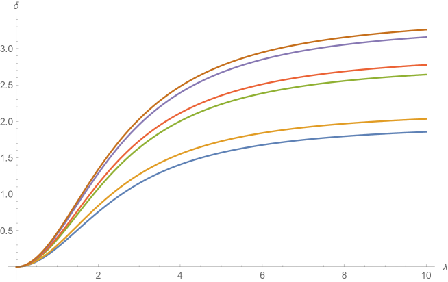
Figure 7: Anomalous dimension of the spin $s$ current, for $s=3,4,5,6,7,8$ as a function of $\lambda_{M}$ (to be multiplied by $M/N$).

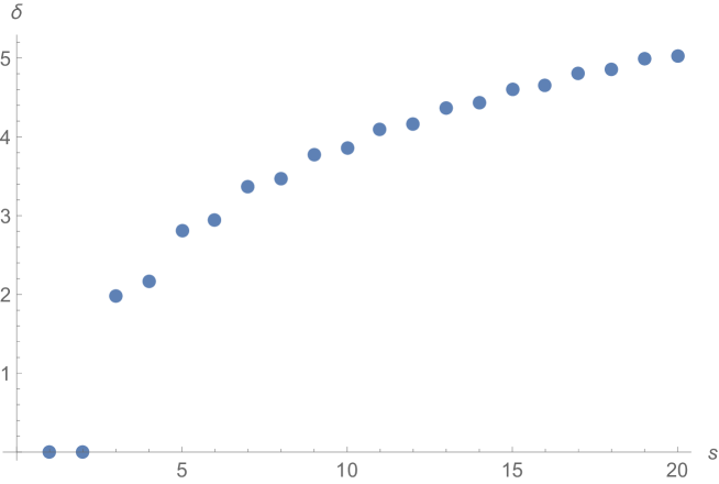
Figure 8: Anomalous dimensions of the current as a function of spin, in the strong coupling limit, (to be multiplied by $M/N$).

5 Large Spin Expansion

In this section, we briefly comment on the large spin expansion of our results and the results of Giombi:2016zwa .

In the large spin limit, our results can be written as:

$$\begin{split}\delta_{s}=&\frac{M}{N}\left(\frac{8\lambda_{M}^{2}}{3\pi^{2}\lambda_{M}^{2}+192}\right)(6\log(4s)+6\gamma-11)\\ &+\frac{M}{N}\left(\frac{\lambda_{M}^{2}}{3\pi^{2}\lambda_{M}^{2}+192}\right)\left(-\frac{4}{s^{2}}-\frac{37}{20s^{4}}-\frac{4}{21s^{6}}+O\left(\frac{1}{s^{7}}\right)\right),\\ &\text{ for odd $s$,}\end{split}$$ (53)

and

$$\begin{split}\delta_{s}=&\frac{M}{N}\left(\frac{8\lambda_{M}^{2}}{3\pi^{2}\lambda_{M}^{2}+192}\right)(6\log(4s)+6\gamma-11)\\ &+\frac{M}{N}\left(\frac{512\lambda_{M}^{2}}{3\left(\pi^{2}\lambda_{M}^{2}+64\right)^{2}}\right)\left(-\frac{25}{2s^{2}}-\frac{3397}{160s^{4}}-\frac{1955}{84s^{6}}+O\left(\frac{1}{s^{7}}\right)\right)\\ &+\frac{M}{N}\left(\frac{8\pi^{2}\lambda_{M}^{4}}{3\left(\pi^{2}\lambda_{M}^{2}+64\right)^{2}}\right)\left(-\frac{3}{s}-\frac{1}{2s^{2}}-\frac{75}{4s^{3}}-\frac{37}{160s^{4}}+O\left(\frac{1}{s^{5}}\right)\right),\\ &\text{ for even $s$.}\end{split}$$ (54)

We presented the anomalous dimension in this way to draw an analogy with equations (61) and (63) of Alday:2015eya , which give the large spin expansion of the large $N$ anomalous dimensions of non-singlet and singlet operators in the critical $O(N)$ model Lang:1992zw ; Lang:1993ge .

The first term in each equation is the $s\rightarrow\infty$ limit of the anomalous dimension, which contains a $\log s$, unlike the critical $O(N)$ model. Hence the anomalous dimension of $\psi$ is undefined, which is expected as it is not a gauge invariant operator.

Looking at the subsequent terms in equations (53) and (54), it appears as if, just as in the critical $O(N)$ model, for odd-spins (which resemble non-singlet operators in the critical $O(N)$ model), the anomalous dimensions are due to an intermediate operator of twist two (i.e., $\bar{\psi}\psi$), while for even spins (which resemble singlet operators in the critical $O(N)$ model) we have two series – the first series corresponding to the twist-two operator and the second series corresponding to twist-one operators (such as $j_{s}$). There may be some ambiguity in separating these two series, and these observations are only suggestive at present because the the analysis of Alday:2015eya does not immediately apply here.

5.1 Conformal Spin

It is also interesting to express these results in terms of the conformal spin $J$ Alday:2015eya , defined as a function of spin $s$ and twist $\tau=\Delta-s$ as:

$$J^{2}=(s+\tau/2-1)(s+\tau/2).$$ (55)

In Alday:2015eya , it was argued that the expansion of anomalous dimensions around large conformal spin should contain only even powers of $1/J$, possibly with extra $\log J$ coefficients. Due to the fact that the field $\psi$ is not a gauge invariant operator, and the dimensionality of space-time is odd, the results of Alday:2015eya do not immediately apply here. However, as will be described elsewhere, applying the ideas of Alday:2015ota ; Alday:2016njk ; Alday:2016jfr , it is possible to refine the arguments of Alday:2015eya to show that this result holds to order $\lambda_{M}^{2}$, but should not be expected to hold at higher orders.

Expanded in powers of $M/N$, the conformal spin is given by

$$J=J_{0}+J_{1}\frac{M}{N}+\ldots.$$ (56)

Because the leading order anomalous dimensions vanish in our theory, $\tau=1+O(\frac{M}{N})$ and $J_{0}$ is given by the free value:

$$J_{0}^{2}=(s+1/2)(s-1/2).$$ (57)

Re-expressing our results in terms of $J=J_{0}+O\left(\frac{M}{N}\right)$, we have, for odd spins:

$$\begin{split}\delta^{\text{odd}}_{s}(J)=&\frac{M}{N}\Bigg{[}\frac{8\lambda_{M}^{2}(-11+6\gamma+12\log(2))}{3\left(\pi^{2}\lambda_{M}^{2}+64\right)}+\frac{16\lambda_{M}^{2}}{64+\pi^{2}\lambda_{M}^{2}}\psi\left(\sqrt{J^{2}+\frac{1}{4}}+\frac{1}{2}\right)\\ &-\frac{2\lambda_{M}^{2}}{\left(\pi^{2}\lambda_{M}^{2}+64\right)}\frac{1}{J^{2}}\Bigg{]},\end{split}$$ (58)

Here $\psi$ denotes the digamma function. Note that

$$\psi\left(\sqrt{J^{2}+\frac{1}{4}}+\frac{1}{2}\right)=\log\left({J}\right)+\frac{1}{6J^{2}}-\frac{1}{30J^{4}}+\frac{4}{315J^{6}}-\frac{1}{105J^{8}}+\ldots$$ (59)

contains only even powers of $1/J$ in its expansion, apart from the initial $\log J$. Hence the entire expression has an expansion in even powers of $1/J$, to all orders in $\lambda_{M}$.

For even spins,

$$\begin{split}\delta_{s}(J)=&\frac{M}{N}\Bigg{[}\frac{8\lambda_{M}^{2}(-11+6\gamma+12\log(2))}{3\left(\pi^{2}\lambda_{M}^{2}+64\right)}+\frac{16\lambda_{M}^{2}}{64+\pi^{2}\lambda_{M}^{2}}\psi\left(\sqrt{J^{2}+\frac{1}{4}}+\frac{1}{2}\right)\\ &-\frac{64\lambda_{M}^{2}}{\left(\pi^{2}\lambda_{M}^{2}+64\right)^{2}}\left[\frac{2\left(68J^{2}+45\right)}{J^{2}(4J^{2}-3)}\right]\\ &-\frac{2\pi^{2}\lambda_{M}^{4}}{\left(\pi^{2}\lambda_{M}^{2}+64\right)^{2}}\left[\frac{(8J^{2}+42)\sqrt{4J^{2}+1}}{J^{2}(4J^{2}-3)}+\frac{1}{J^{2}}\right]\Bigg{]}.\end{split}$$ (60)

Here, we see that the last piece would contain even as well as odd powers of $1/J$. This corresponds to an order $\lambda_{M}^{4}$ correction, so at order $\lambda_{M}^{2}$, we again get an expansion with only even powers of $1/J$. The odd powers of $1/J$ originate from a term proportional to $\sqrt{4J^{2}+1}$, and could be interpreted as originating from the exchange of a tower of twist-one (almost-conserved) operators. Such a term is also present in the singlet large $N$ anomalous dimensions of the critical $O(N)$ model in $d=3$, given in equation (64) of Alday:2015eya .

6 Discussion

In this paper, we studied the $M/N$ anomalous dimensions in a bifundamental $U(N)\times U(M)$ Chern-Simons theory, $\delta_{s}(\lambda_{M},\lambda_{N})$, in the special case $\lambda_{N}=0$. These results compliment the results of Giombi:2016zwa , which effectively determine the anomalous dimensions in the case $\lambda_{M}=0$. It should also be possible to determine the $M/N$ anomalous dimensions in the bifundamental theory to all orders in both $\lambda_{M}$ and $\lambda_{N}$ by extending the arguments given in section 3, however, the calculation would be substantially more involved. We hope to address this problem in the near future.

Chern-Simons theories coupled to matter have also played an important role in the study of fractional quantum Hall transitions, e.g., WenWu ; Mott ; Hui:2017pwe . In particular, Mott includes a study of $U(1)$-Chern Simons theory coupled to $N$ flavours of fermions as a model of a Mott Insulator -quantum Hall transition, which, at the level of $1/N$ corrections also has the same spectrum as the $U(M)$ theory we consider. The anomalous dimension of the scalar operator $\bar{\psi}\psi$ effectively determines the critical exponent $\nu$ associated with the transition, and so is of experimental interest. To date, the anomalous dimension of $\bar{\psi}\psi$ in the large colour theory is not known, and it would be interesting to compare the value of $\nu$ from this calculation to the existing large flavour calculation.

We are not aware if the anomalous dimension of the higher-spin currents have any similar physical interpretation or relevance to Quantum Hall physics, but it may be interesting to pursue this further. It might also be possible to study the spectrum at order $1/N^{2}$, which may perhaps provide better agreement with experiment (in which $N=1$). The techniques involved would be similar to the recent computations of $1/N^{2}$ spectrum of the critical $O(N)$ and Gross-Neveu models Manashov:2016uam ; Manashov:2017xtt . Correlation functions involving the stress tensor and conserved $U(1)$ current could also be calculated in this theory possibly at finite temperature/chemical potential (e.g., Geracie:2015drf ), and may correspond to physical observables. These should obey the bounds determined in Hofman:2008ar ; Chowdhury:2016hjy ; Chowdhury:2017vel ; Cordova:2017zej .

It would also be of interest to consider scaling dimensions in the theory of $U(M)_{k}$ Chern-Simons coupled to $N$ critical bosons, when $N$ is large. In WenWu , the anomalous dimension of the scalar operator $j_{0}$ was calculated in the $U(1)$ version of this theory. It would be interesting to also compute the higher spin spectrum and compare it is to the spectrum of the fermionic theory studied here.

Chern-Simons theories coupled to matter also exhibit a beautiful bosonization duality Aharony:2012nh relating theories with fermionic matter to critical bosonic matter. This duality was discovered and has been supported via various large $N$ computations MZ ; GurAri:2012is ; Aharony:2012ns ; Jain:2013py ; Jain:2013gza ; Jain:2014nza ; Bedhotiya:2015uga ; Gur-Ari:2015pca ; Yokoyama:2016sbx ; Minwalla:2015sca ; Gur-Ari:2015pca , but it is now conjectured to hold at finite $N$ as well Aharony:2015mjs ; Kachru:2016rui ; Kachru:2016aon ; Hsin:2016blu ; Aharony:2016jvv , and has been of interest from the point of view of condensed matter (e.g., Seiberg:2016gmd ; Karch:2016sxi ; Murugan:2016zal ; Metlitski:2016dht ). These dualities can be thought of as generalizations of the supersymmetric Giveon-Kutasov duality Giveon:2008zn ; Kapustin:2011gh ; Benini:2011mf ; Intriligator:2013lca . While these dualities cannot hold in the large flavour limit, they may perhaps be generalized to bifundamental Chern-Simons theories when both couplings are nonzero, as a strong/weak duality when $\lambda_{N}\leftrightarrow(1-|\lambda_{N}|)$. One form for these dualites was conjectured in Gurucharan:2014cva , based on analogy with ABJ dualities Aharony:2008gk , and could be tested by explicit computation when $M\ll N$ in the fermionic and critical bosonic theory. (Some perturbative calculations in the non-critical bifundamental bosonic theory appear in Banerjee:2013nca .) We hope to perform these tests in the near future.

Finally, we found the spectrum of anomalous dimensions appears to take a form similar to those of the large $N$ critical $O(N)$ model, when expanded in a large spin expansion, and also expressed in terms of conformal spin, despite the additional logarithmic dependence on spin. It would be interesting if this behaviour could be better understood from the point of view of large spin perturbation theory, e.g., Alday:2015eya ; Alday:2015ota ; Alday:2016njk ; Alday:2016jfr .

References

- (1) S. Giombi, S. Minwalla, S. Prakash, S. P. Trivedi, S. R. Wadia et al., Chern-Simons Theory with Vector Fermion Matter, Eur.Phys.J. C72 (2012) 2112, [1110.4386].
- (2) X.-G. Wen and Y.-S. Wu, Transitions between the quantum hall states and insulators induced by periodic potentials, Phys. Rev. Lett. 70 (Mar, 1993) 1501–1504.
- (3) W. Chen, M. P. A. Fisher and Y.-S. Wu, Mott transition in an anyon gas, Phys. Rev. B 48 (Nov, 1993) 13749–13761.
- (4) A. Hui, M. Mulligan and E.-A. Kim, Non-Abelian Fermionization and Fractional Quantum Hall Transitions, 1710.11137.
- (5) M. Moshe and J. Zinn-Justin, Quantum field theory in the large N limit: A Review, Phys. Rept. 385 (2003) 69–228, [hep-th/0306133].
- (6) T. Muta and D. S. Popovic, Anomalous Dimensions of Composite Operators in the Gross-Neveu Model in Two + Epsilon Dimensions, Prog. Theor. Phys. 57 (1977) 1705.
- (7) K. Lang and W. Ruhl, The Critical O(N) sigma model at dimensions 2 < d < 4: Fusion coefficients and anomalous dimensions, Nucl. Phys. B400 (1993) 597–623.
- (8) K. Lang and W. Ruhl, Critical O(N) vector nonlinear sigma models: A Resume of their field structure, 1993, hep-th/9311046.
- (9) S. Giombi and V. Kirilin, Anomalous Dimensions in CFT with Weakly Broken Higher Spin Symmetry, 1601.01310.
- (10) Y. Hikida, The masses of higher spin fields on and conformal perturbation theory, Phys. Rev. D94 (2016) 026004, [1601.01784].
- (11) K. Nii, Classical equation of motion and Anomalous dimensions at leading order, JHEP 07 (2016) 107, [1605.08868].
- (12) Y. Hikida and T. Wada, Anomalous dimensions of higher spin currents in large N CFTs, 1610.05878.
- (13) A. N. Manashov and E. D. Skvortsov, Higher-spin currents in the Gross-Neveu model at , 1610.06938.
- (14) S. Giombi, V. Kirilin and E. Skvortsov, Notes on Spinning Operators in Fermionic CFT, JHEP 05 (2017) 041, [1701.06997].
- (15) A. N. Manashov, E. D. Skvortsov and M. Strohmaier, Higher spin currents in the critical ) vector model at , JHEP 08 (2017) 106, [1706.09256].
- (16) T. W. Appelquist, M. J. Bowick, D. Karabali and L. C. R. Wijewardhana, Spontaneous Chiral Symmetry Breaking in Three-Dimensional QED, Phys. Rev. D33 (1986) 3704.
- (17) T. Appelquist, M. J. Bowick, D. Karabali and L. C. R. Wijewardhana, Spontaneous Breaking of Parity in (2+1)-dimensional QED, Phys. Rev. D33 (1986) 3774.
- (18) T. Appelquist, D. Nash and L. Wijewardhana, Critical Behavior in (2+1)-Dimensional QED, Phys.Rev.Lett. 60 (1988) 2575.
- (19) T. Appelquist and D. Nash, Critical Behavior in (2+1)-dimensional QCD, Phys. Rev. Lett. 64 (1990) 721.
- (20) W. Rantner and X.-G. Wen, Spin correlations in the algebraic spin liquid: Implications for high-tc superconductors, Phys. Rev. B 66 (Oct, 2002) 144501.
- (21) S. S. Pufu, Anomalous dimensions of monopole operators in three-dimensional quantum electrodynamics, Phys.Rev. D89 (2014) 065016, [1303.6125].
- (22) R. Rattazzi, V. S. Rychkov, E. Tonni and A. Vichi, Bounding scalar operator dimensions in 4D CFT, JHEP 12 (2008) 031, [0807.0004].
- (23) R. Gopakumar, A. Kaviraj, K. Sen and A. Sinha, Conformal Bootstrap in Mellin Space, 1609.00572.
- (24) P. Dey, A. Kaviraj and K. Sen, More on analytic bootstrap for O(N) models, JHEP 06 (2016) 136, [1602.04928].
- (25) A. M. Polyakov, Conformal symmetry of critical fluctuations, JETP Lett. 12 (1970) 381–383.
- (26) A. L. Fitzpatrick, J. Kaplan, D. Poland and D. Simmons-Duffin, The Analytic Bootstrap and AdS Superhorizon Locality, JHEP 1312 (2013) 004, [1212.3616].
- (27) Z. Komargodski and A. Zhiboedov, Convexity and Liberation at Large Spin, JHEP 11 (2013) 140, [1212.4103].
- (28) L. F. Alday and A. Bissi, Higher-spin correlators, JHEP 10 (2013) 202, [1305.4604].
- (29) A. Kaviraj, K. Sen and A. Sinha, Analytic bootstrap at large spin, JHEP 11 (2015) 083, [1502.01437].
- (30) L. F. Alday, A. Bissi and T. Lukowski, Large spin systematics in CFT, JHEP 11 (2015) 101, [1502.07707].
- (31) A. Kaviraj, K. Sen and A. Sinha, Universal anomalous dimensions at large spin and large twist, JHEP 07 (2015) 026, [1504.00772].
- (32) L. F. Alday and A. Zhiboedov, Conformal Bootstrap With Slightly Broken Higher Spin Symmetry, JHEP 06 (2016) 091, [1506.04659].
- (33) E. D. Skvortsov, On (Un)Broken Higher-Spin Symmetry in Vector Models, 1512.05994.
- (34) A. Dymarsky, I. R. Klebanov and R. Roiban, Perturbative search for fixed lines in large N gauge theories, JHEP 08 (2005) 011, [hep-th/0505099].
- (35) V. Gurucharan and S. Prakash, Anomalous dimensions in non-supersymmetric bifundamental Chern-Simons theories, JHEP 09 (2014) 009, [1404.7849].
- (36) C.-M. Chang and X. Yin, Higher Spin Gravity with Matter in AdS_3 and Its CFT Dual, 1106.2580.
- (37) O. Aharony, O. Bergman, D. L. Jafferis and J. Maldacena, N=6 superconformal Chern-Simons-matter theories, M2-branes and their gravity duals, JHEP 0810 (2008) 091, [0806.1218].
- (38) O. Aharony, O. Bergman and D. L. Jafferis, Fractional M2-branes, JHEP 0811 (2008) 043, [0807.4924].
- (39) M. Honda, Y. Pang and Y. Zhu, ABJ Quadrality, JHEP 11 (2017) 190, [1708.08472].
- (40) C.-M. Chang, S. Minwalla, T. Sharma and X. Yin, ABJ Triality: from Higher Spin Fields to Strings, J.Phys. A46 (2013) 214009, [1207.4485].
- (41) J. Maldacena and A. Zhiboedov, Constraining conformal field theories with a slightly broken higher spin symmetry, Class.Quant.Grav. 30 (2013) 104003, [1204.3882].
- (42) G. Gur-Ari and R. Yacoby, Correlators of Large N Fermionic Chern-Simons Vector Models, JHEP 1302 (2013) 150, [1211.1866].
- (43) O. Aharony, S. Giombi, G. Gur-Ari, J. Maldacena and R. Yacoby, The Thermal Free Energy in Large N Chern-Simons-Matter Theories, 1211.4843.
- (44) S. Jain, S. Minwalla, T. Sharma, T. Takimi, S. R. Wadia and S. Yokoyama, Phases of large vector Chern-Simons theories on , JHEP 09 (2013) 009, [1301.6169].
- (45) S. Jain, S. Minwalla and S. Yokoyama, Chern Simons duality with a fundamental boson and fermion, JHEP 1311 (2013) 037, [1305.7235].
- (46) S. Jain, M. Mandlik, S. Minwalla, T. Takimi, S. R. Wadia and S. Yokoyama, Unitarity, Crossing Symmetry and Duality of the S-matrix in large N Chern-Simons theories with fundamental matter, JHEP 04 (2015) 129, [1404.6373].
- (47) A. Bedhotiya and S. Prakash, A test of bosonization at the level of four-point functions in Chern-Simons vector models, JHEP 12 (2015) 032, [1506.05412].
- (48) G. Gur-Ari and R. Yacoby, Three Dimensional Bosonization From Supersymmetry, JHEP 11 (2015) 013, [1507.04378].
- (49) S. Yokoyama, Scattering Amplitude and Bosonization Duality in General Chern-Simons Vector Models, JHEP 09 (2016) 105, [1604.01897].
- (50) S. Minwalla and S. Yokoyama, Chern Simons Bosonization along RG Flows, JHEP 02 (2016) 103, [1507.04546].
- (51) K. Inbasekar, S. Jain, P. Nayak and V. Umesh, All tree level scattering amplitudes in Chern-Simons theories with fundamental matter, 1710.04227.
- (52) K. Inbasekar, S. Jain, S. Majumdar, P. Nayak, T. Neogi, T. Sharma et al., Dual Superconformal Symmetry of Chern-Simons theory with Fundamental Matter and Non-Renormalization at Large , 1711.02672.
- (53) K. Inbasekar, S. Jain, S. Mazumdar, S. Minwalla, V. Umesh and S. Yokoyama, Unitarity, crossing symmetry and duality in the scattering of susy matter Chern-Simons theories, JHEP 10 (2015) 176, [1505.06571].
- (54) O. Aharony, G. Gur-Ari and R. Yacoby, d=3 Bosonic Vector Models Coupled to Chern-Simons Gauge Theories, JHEP 1203 (2012) 037, [1110.4382].
- (55) I. Klebanov and A. Polyakov, AdS dual of the critical O(N) vector model, Phys.Lett. B550 (2002) 213–219, [hep-th/0210114].
- (56) E. Sezgin and P. Sundell, Massless higher spins and holography, Nucl.Phys. B644 (2002) 303–370, [hep-th/0205131].
- (57) C. Sleight and M. Taronna, Higher-Spin Algebras, Holography and Flat Space, JHEP 02 (2017) 095, [1609.00991].
- (58) E. Sezgin and P. Sundell, Holography in 4D (super) higher spin theories and a test via cubic scalar couplings, JHEP 0507 (2005) 044, [hep-th/0305040].
- (59) S. Giombi and X. Yin, Higher Spin Gauge Theory and Holography: The Three-Point Functions, JHEP 1009 (2010) 115, [0912.3462].
- (60) S. Giombi and X. Yin, Higher Spins in AdS and Twistorial Holography, JHEP 1104 (2011) 086, [1004.3736].
- (61) S. Giombi and X. Yin, On Higher Spin Gauge Theory and the Critical O(N) Model, 1105.4011.
- (62) S. Giombi, Higher Spin — CFT Duality, in Proceedings, Theoretical Advanced Study Institute in Elementary Particle Physics: New Frontiers in Fields and Strings (TASI 2015): Boulder, CO, USA, June 1-26, 2015, pp. 137–214, 2017, 1607.02967, DOI.
- (63) E. Sezgin, E. D. Skvortsov and Y. Zhu, Chern-Simons Matter Theories and Higher Spin Gravity, JHEP 07 (2017) 133, [1705.03197].
- (64) V. E. Didenko and M. A. Vasiliev, Test of the local form of higher-spin equations via AdS/CFT, 1705.03440.
- (65) J. M. Maldacena, The Large N limit of superconformal field theories and supergravity, Adv.Theor.Math.Phys. 2 (1998) 231–252, [hep-th/9711200].
- (66) S. Giombi, V. Gurucharan, V. Kirilin, S. Prakash and E. Skvortsov, On the Higher-Spin Spectrum in Large N Chern-Simons Vector Models, JHEP 01 (2017) 058, [1610.08472].
- (67) J. Maldacena and A. Zhiboedov, Constraining Conformal Field Theories with A Higher Spin Symmetry, J.Phys. A46 (2013) 214011, [1112.1016].
- (68) J. Maldacena and A. Zhiboedov, Constraining conformal field theories with a slightly broken higher spin symmetry, Class. Quant. Grav. 30 (2013) 104003, [1204.3882].
- (69) L. F. Alday and J. M. Maldacena, Comments on operators with large spin, JHEP 11 (2007) 019, [0708.0672].
- (70) M. S. Costa, J. Penedones, D. Poland and S. Rychkov, Spinning Conformal Correlators, JHEP 11 (2011) 071, [1107.3554].
- (71) S. Giombi, S. Prakash and X. Yin, A Note on CFT Correlators in Three Dimensions, JHEP 1307 (2013) 105, [1104.4317].
- (72) L. F. Alday, Large Spin Perturbation Theory for Conformal Field Theories, Phys. Rev. Lett. 119 (2017) 111601, [1611.01500].
- (73) L. F. Alday, Solving CFTs with Weakly Broken Higher Spin Symmetry, 1612.00696.
- (74) M. Geracie, M. Goykhman and D. T. Son, Dense Chern-Simons Matter with Fermions at Large N, JHEP 04 (2016) 103, [1511.04772].
- (75) D. M. Hofman and J. Maldacena, Conformal collider physics: Energy and charge correlations, JHEP 05 (2008) 012, [0803.1467].
- (76) S. D. Chowdhury, J. R. David and S. Prakash, Spectral sum rules for conformal field theories in arbitrary dimensions, JHEP 07 (2017) 119, [1612.00609].
- (77) S. D. Chowdhury, J. R. David and S. Prakash, Constraints on parity violating conformal field theories in , 1707.03007.
- (78) C. Cordova, J. Maldacena and G. J. Turiaci, Bounds on OPE Coefficients from Interference Effects in the Conformal Collider, 1710.03199.
- (79) O. Aharony, G. Gur-Ari and R. Yacoby, Correlation Functions of Large N Chern-Simons-Matter Theories and Bosonization in Three Dimensions, JHEP 1212 (2012) 028, [1207.4593].
- (80) O. Aharony, Baryons, monopoles and dualities in Chern-Simons-matter theories, JHEP 02 (2016) 093, [1512.00161].
- (81) S. Kachru, M. Mulligan, G. Torroba and H. Wang, Bosonization and Mirror Symmetry, Phys. Rev. D94 (2016) 085009, [1608.05077].
- (82) S. Kachru, M. Mulligan, G. Torroba and H. Wang, Nonsupersymmetric dualities from mirror symmetry, Phys. Rev. Lett. 118 (2017) 011602, [1609.02149].
- (83) P.-S. Hsin and N. Seiberg, Level/rank Duality and Chern-Simons-Matter Theories, JHEP 09 (2016) 095, [1607.07457].
- (84) O. Aharony, F. Benini, P.-S. Hsin and N. Seiberg, Chern-Simons-matter dualities with and gauge groups, JHEP 02 (2017) 072, [1611.07874].
- (85) N. Seiberg, T. Senthil, C. Wang and E. Witten, A Duality Web in 2+1 Dimensions and Condensed Matter Physics, Annals Phys. 374 (2016) 395–433, [1606.01989].
- (86) A. Karch and D. Tong, Particle-Vortex Duality from 3d Bosonization, Phys. Rev. X6 (2016) 031043, [1606.01893].
- (87) J. Murugan and H. Nastase, Particle-vortex duality in topological insulators and superconductors, JHEP 05 (2017) 159, [1606.01912].
- (88) M. A. Metlitski, A. Vishwanath and C. Xu, Duality and bosonization of (2+1) -dimensional Majorana fermions, Phys. Rev. B95 (2017) 205137, [1611.05049].
- (89) A. Giveon and D. Kutasov, Seiberg Duality in Chern-Simons Theory, Nucl.Phys. B812 (2009) 1–11, [0808.0360].
- (90) A. Kapustin, Seiberg-like duality in three dimensions for orthogonal gauge groups, 1104.0466.
- (91) F. Benini, C. Closset and S. Cremonesi, Comments on 3d Seiberg-like dualities, JHEP 1110 (2011) 075, [1108.5373].
- (92) K. Intriligator and N. Seiberg, Aspects of 3d N=2 Chern-Simons-Matter Theories, JHEP 07 (2013) 079, [1305.1633].
- (93) S. Banerjee and D. Radicevic, Chern-Simons theory coupled to bifundamental scalars, JHEP 06 (2014) 168, [1308.2077].