A nestable, multigrid-friendly grid on a sphere for global spectral models based on Clenshaw-Curtis quadrature

Abstract

A new grid system on a sphere is proposed that allows for straightforward implementation of both spherical-harmonics-based spectral methods and gridpoint-based multigrid methods. The latitudinal gridpoints in the new grid are equidistant and spectral transforms in the latitudinal direction are performed using Clenshaw-Curtis quadrature. The spectral transforms with this new grid and quadrature are shown to be exact within the machine precision provided that the grid truncation is such that there are at least $2N+1$ latitudinal gridpoints for the total truncation wavenumber of $N$. The new grid and quadrature is implemented and tested on a shallow-water equations model and the hydrostatic dry dynamical core of the global NWP model JMA-GSM. The integration results obtained with the new quadrature are shown to be almost identical to those obtained with the conventional Gaussian quadrature on Gaussian grid. Only minor code changes are required to adapt any Gaussian-based spectral models to employ the proposed quadrature.

This is the peer reviewed version of the following article: Hotta and Ujiie (2018) QJRMS144(714) 1382–1397, which has been published in final form at
https://doi.org/10.1002/qj.3282. This article may be used for non-commercial purposes in accordance with Wiley Terms and Conditions for Self-Archiving.

1 Introduction

Global spectral atmospheric models that are in use today almost universally adopt Gaussian quadrature in the meridional direction to perform forward (gridpoint-to-wavenumber) spherical harmonics transform. Gaussian quadrature is an optimal quadrature rule in the sense of maximising the degree of polynomials that can be integrated exactly for a given number of quadrature points (or nodes). Given $J$ nodes, Gaussian quadrature is exact for integrand polynomials of up to as high as $2J-1$ degrees. This optimality is achieved, however, with several inconveniences (e.g. Clenshaw and Curtis, 1960): First, the nodes and weights are not given in an explicit analytic form and necessitates (some iterative) solution of an algebraic equation of high degrees. Second, the nodes do not nest, i.e., the nodes for the $J$-point rule do not contain any $J^{\prime}$-point nodes as their subset for any $J^{\prime}<J$. While the former is now not so much an inconvenience than it used to be thanks to the recently developed elegant, fast and yet accurate computing methods (e.g., Hale and Townsend, 2013, and the other algorithms reviewed in Townsend, 2015), all the more so in the context of atmospheric modelling since the quadrature nodes and weights can be pre-computed once at the initialisation process and stored in memory to be reused during the subsequent time integration steps, the latter limitation does impose some inflexibility to the future evolution of a global spectral dynamical core. In particular, the unnestable grid alignment makes it cumbersome, if not impracticable, to combine the current spectral dynamical core with a multigrid approach for solving an elliptic boundary value problem that arises from (semi-)implicit time discretisation.

As the horizontal resolution continues to increase, it becomes necessary to properly represent nature’s non-hydrostatic aspects in the model. In a non-hydrostatic system, a semi-implicit time stepping results in a Helmholtz problem with spatially-variable coefficients that needs to be solved iteratively, even with horizontal spectral discretisation (e.g., Bénard, 2004). This is in contrast to the hydrostatic case where the resultant Helmholtz problem has constant coefficients and thus can be solved without iteration in the spectral space (Hoskins and Simmons, 1975).

The multigrid approach is an attractive strategy for iterative solution of the non-hydrostatic implicit Helmholtz problem. It accelerates convergence of the iterative algorithm by first solving the problem at a lower resolution and then gradually increasing the resolution, ingesting the solution from the previous (lower) resolution as the initial guess to the next (higher) resolution. While such an approach has been applied and proved effective in the context of grid-based atmospheric models (e.g. Heikes et al., 2013; Sandbach et al., 2015), implementing it on current spectral models is not straightforward because the aforementioned non-nested nature of Gaussian quadrature necessitates some form of accurate off-grid interpolation (e.g., Jones, 1999; Ullrich et al., 2009) from higher- to lower-resolution grid (and vice versa). See Appendix C for further discussion.

Another spectrally accurate family of quadrature rules exist, however, that, unlike the conventional Gaussian quadrature, have nestable nodes that would allow for straightforward implementation of multigrid approach. These quadrature rules, introduced by Fejér (1933) and Clenshaw and Curtis (1960), have been well known in the field of Numerical Analysis and are shown by some authors to have several advantages over the classical Gaussian quadrature. Although Clenshaw-Curtis or Fejér quadrature rules are not optimal in the sense of giving exact integration for polynomials of up to only $J-1$ (as opposed to the Gaussian $2J-1$) degrees given $J$ nodes, they have been shown to be practically as accurate as Gaussian quadrature in many applications (e.g. Trefethen, 2008, and the references therein). Despite gaining popularity in numerical analysis, to the authors’ best knowledge, Clenshaw-Curtis-type quadrature appears not to have been used in spectral transform models, at least in atmospheric modelling.

In this paper we aim to show that the Clenshaw-Curtis quadrature, with its associated nodes (which turn out to be just equispaced latitude grids, see (13)), can be used as an alternative to the classical Gaussian quadrature with the Gaussian latitude grids in atmospheric global spectral models. Although our ultimate goal is to investigate the effectiveness of a multigrid approach in a global non-hydrostatic spectral model defined on the multigrid-friendly Clenshaw-Curtis grid, we defer actual multigrid implementation to future work and limit the scope of the present paper to only showing numerical soundness of the quadrature applied to the associated Legendre functions and the equivalence of the Gaussian and Clenshaw-Curtis quadrature implemented on a shallow-water equations (SWE) model and a three-dimensional dry hydrostatic primitive equations (HPE) model. To clarify our motivation, we provide, in Appendix C, a rough outline on how the proposed quadrature and grid will aid in multigrid implementation.

The rest of the paper is structured as follows: Section 2 reminds the reader with how the quadrature is used in global spectral atmospheric models. Section 3 introduces Clenshaw-Curtis quadrature in the context of spectral transform. Section 4 examines the numerical orthonormality of the associated Legendre functions evaluated with Clenshaw-Curtis quadrature with a comment on aliasing of quadratic and cubic terms. Sections 5 and 6 document the implementation of Clenshaw-Curtis quadrature to the spherical SWE model and the HPE global dynamical core, and compare the results produced with Gaussian and Clenshaw-Curtis quadrature in the context of standardised test cases. Section 7 concludes the paper with an outlook for our future plans.

2 Discrete spherical harmonics transforms and Gaussian quadrature

Global spectral models represent atmospheric state variables in both gridpoint space and wavenumber (spectral) space and transform them back and forth during the course of time integration (Orszag, 1970).

The discrete inverse spherical harmonics transform, or synthesis, transforms the state variable from the spectral representation $X_{n}^{m}$ to its gridpoint-space representation $X(\lambda_{i},\phi_{j})$ by the following formula:

$$X(\lambda_{i},\phi_{j}) = \sum_{m=-N}^{N}\sum_{n=|m|}^{N}X_{n}^{m}Y_{n}^{m}(\lambda_{i},\phi_{j})$$ (1)

where $N$ is the truncation total wavenumber, $n$ and $m$ are, respectively, the total and zonal wavenumber, $\lambda$ is the longitude, $\phi$ is the latitude, $Y_{n}^{m}(\lambda,\phi)$ is the spherical harmonic function with the total and zonal wavenumbers of $n$ and $m$, respectively. Throughout this manuscript, the triangular truncation as in (1) is assumed. In the Japan Meteorological Agency (JMA)’s Global Spectral Model (JMA-GSM), as in other spectral models, the transform of (1) is implemented via two steps by first performing the associated Legendre transform in the meridional direction from $X_{n}^{m}$ to

$$X^{m}(\phi_{j}):=\sum_{n=|m|}^{N}X_{n}^{m}\tilde{P}_{n}^{m}(\sin\phi_{j})$$ (2)

and then performing inverse discrete Fourier transform (DFT) in the zonal direction from $X^{m}(\phi_{j})$ to $X(\lambda_{i},\phi_{j}):=\sum_{m=-N}^{N}X^{m}(\phi_{j})e^{\sqrt{-1}\lambda_{i}}$. Here, $\tilde{P}_{n}^{m}(\sin\phi_{j})$ denotes the associated Legendre polynomial of degree $n$ and order $m$, normalised to satisfy the following orthonormality:

$$\int_{-\frac{\pi}{2}}^{\frac{\pi}{2}}\tilde{P}_{n}^{m}(\sin\phi)\tilde{P}_{n^{\prime}}^{m}(\sin\phi)\cos(\phi)d\phi=\delta_{n,n^{\prime}}.$$ (3)

The longitudinal gridpoints $\{\lambda_{i}\},i=0,\cdots,I-1$ are chosen so that the DFT can be computed efficiently via a Fast Fourier Transform (FFT) algorithm, resulting in equispaced grids $\lambda_{i}=2\pi i/I$.

The direct spherical harmonics transform, or analysis, recovers spectral coefficients $X_{n}^{m}$ from the gridpoint-space representation $X(\lambda_{i},\phi_{j})$, by exploiting the orthonormality of the spherical harmonics:

$$X_{n}^{m} = \int_{-\frac{\pi}{2}}^{\frac{\pi}{2}}\int_{0}^{2\pi}X(\lambda,\phi){Y_{n}^{m}}^{*}(\lambda,\phi)d\lambda\cos{\phi}d\phi$$ (4)

$$= \int_{-1}^{1}X^{m}(\phi)\tilde{P}_{n}^{m}(\sin\phi)d\left(\sin\phi\right)$$ (5)

with

$$X^{m}(\phi)=\int_{0}^{2\pi}X(\lambda,\phi)e^{-\sqrt{-1}m\lambda}d\lambda$$ (6)

The integrations in (5-6) have to be evaluated numerically with some quadrature rules. For the zonal direction, direct DFT gives exact integration to an integrand with wavenumbers up to $I$ given $I$ zonal grids. Thus, for each meridional gridpoint $\phi_{j}$, (6) can be discretised as

$$X^{m}(\phi_{j}) = \frac{1}{I}\sum_{i=0}^{I-1}X(\lambda_{i},\phi_{j})e^{-\sqrt{-1}m\lambda_{i}}$$ (7)

with the constraint

$$I>2N$$ (8)

to avoid aliasing introduced by quadrature error (note that the integrand of (6) contains zonal wavenumbers of at most $2N$ because $X(\lambda,\phi)$ is a truncated sum of $Y_{n}^{m}$ with $|m|$ being at most $N$). For the meridional direction, any quadrature rule can be used as long as it gives exact integration to polynomials of $\sin\phi$ to a desired degree. In practice, however, Gaussian quadrature (with the ordinary Legendre polynomials as the basis set) is almost always employed due to its optimality in the sense described in the first paragraph of Section 1. With Gaussian quadrature, (5) is discretised as

$$X_{n}^{m} = \sum_{j=1}^{J}X^{m}(\phi_{j})\tilde{P}_{n}^{m}(\sin\phi_{j})w^{G}_{j}$$ (9)

with the Gaussian weights given by

$$w^{G}_{j} = \frac{2}{JP^{\prime}_{J}(\sin\phi_{j})P_{J-1}(\sin\phi_{j})}$$ (10)

and the latitude grid (the Gaussian latitudes) $\{\phi_{j}\},j=1,\cdots,J$ given as the $J$ roots of $P_{J}(\sin\phi)=0$ where $P_{J}(\sin\phi)$ is the ordinary Legendre polynomial of degree $J$ (NIST, 2016). We remark that several exquisitely fast and accurate algorithms for computing the Gaussian latitudes $\phi_{j}$ and weights $w^{G}_{j}$ have been recently worked out by numerical analysts. Unlike the classical methods employed in atmospheric models that are based on Newton iteration (e.g., Swartztrauber, 2002; Enomoto, 2015) or tridiagonal eigen-solution (Adams and Swartztrauber, 1997), the recently developed methods exploit very accurate asymptotic expansions on $P_{n}(\sin\phi)$ and other related functions and prove particularly useful for high-resolution modelling with large $J$. Notably, Bogaert (2014) successfully derived asymptotic expressions for $\phi_{j}$ and $w^{G}_{j}$ that are accurate enough to allow iteration-free evaluation of them with errors below double-precision machine epsilon; see Townsend (2015) for a historical review.

In order to avoid aliasing due to quadrature errors, there should be at least

$$J\geq(2N+1)/2$$ (11)

latitudinal gridpoints for the given truncation total wavenumber $N$ . This is because the integrand of (5) is a polynomial of $\sin\phi$ of at most $2N$ degree. This condition, along with (8), allows exact discrete transforms with linear truncation (i.e., $J\approx N$).

3 Clenshaw-Curtis quadrature

In numerically evaluating the integration in (5), it is possible, though apparently never have been tried with global spectral models, to use a quadrature rule other than the classical Gaussian formula (9–10). In this paper we focus on using one variant of Clenshaw-Curtis-type quadrature in place of the standard Gaussian quadrature, motivated by its nestable property that we described in Introduction. The quadrature rule we use, whose nodes (13) do not contain the poles, should probably be more appropriately called Fejér quadrature of second kind (Fejér, 1933; Waldvogel, 2006; Trefethen, 2008). Following Boyd (1987), however, in this manuscript we shall abusively call it Clenshaw-Curtis quadrature.

3.1 Formulation

For convenience, we denote the integrand of (5) by

$$g(\cos\theta):=f(\sin\phi):=X^{m}(\phi)\tilde{P}_{n}^{m}(\sin\phi)$$ (12)

where we have introduced the colatitude $\theta=\frac{\pi}{2}-\phi$. Clenshaw-Curtis-type quadrature rules first expand $g(\cos\theta)$ into some trigonometric series and then analytically integrate them term-by-term. The choice of trigonometric base functions specifies the quadrature points and the weights. In atmospheric modelling, more specifically in transitioning from a spherical harmonics transform model based on Gaussian quadrature, it is desirable to avoid placing quadrature points on the poles (c.f., section 3.4). We therefore choose to expand $g(\cos\theta)$ into Chebyshev polynomials of the second kind $U_{l}(\cos\theta)=\sin{(l+1)\theta}/\sin{\theta}$ of degrees $l=0,1,\cdots,J-1$, or equivalently, to expand $g(\cos\theta)\sin\theta$ into the sine series $\sum_{p=1}^{J}a_{p}\sin{p\theta}$, which can be achieved by performing the type-I discrete sine transform (DST) on $g(\cos\theta_{j})\sin\theta_{j}$ without introducing any errors but rounding. From this constraint, the collocation points $\theta_{j}$ (or $\phi_{j}$) are chosen as

$$\theta_{j}=\frac{j}{J+1}\pi,\phi_{j}=\frac{\pi}{2}\left(1-\frac{2j}{J+1}\right),j=1,2,\cdots,J$$ (13)

Note here that the poles ($j=0$ and $j=J+1$) are absent, which is exactly what motivated us to choose $U_{l}(\cos\theta)$ as the base functions.

As pointed out by Gentleman (1972a,1972b), the type-I DST in expanding $g(\cos\theta)$ into Chebyshev polynomials $U_{l}(\cos{\theta})$ can be efficiently implemented by FFT, allowing quadrature to be performed with $O(J\log{J})$ operations without explicit computation of the quadrature weights. While this is advantageous if a single execution of quadrature is concerned, this is not the case for spherical-harmonics-based global spectral models where the quadrature of the form of (5) is repeated $O(N^{2})$ times on each spectral transform and the weights can be pre-computed and stored in memory to be reused many times. From the viewpoint of adapting the code from the existing one based on Gaussian quadrature, it is favourable if the quadrature can be expressed in the standard interpolative form analogous to (9) rather than to rely on FFT (or DST) code. Boyd (1987) showed that this is possible. He showed that the quadrature can be cast in the following standard quadrature form:

$$\int_{-1}^{1}f(\sin\phi)d\left(\sin\phi\right) = \sum_{j=1}^{J}f(\sin\phi_{j})w^{CC}_{j}$$ (14)

$$= \sum_{j=1}^{J}X^{m}(\phi_{j})\tilde{P}_{n}^{m}(\sin\phi_{j})w^{CC}_{j}$$ (15)

with the weights $w^{CC}_{j}$ given by

$$w^{CC}_{j}=\frac{4\sin\theta_{j}}{J+1}\sum_{\begin{subarray}{c}1\leq p\leq J\\ p\mathrm{:\ odd}\end{subarray}}\frac{\sin\left(p\theta_{j}\right)}{p}.$$ (16)

Boyd (1987) did not provide explicit derivation of (16); we give a concise derivation in Appendix A. Computing the Clenshaw-Curtis weights from (16) involves $O(J^{2})$ operations. This is usually not a significant burden for atmospheric models since the weights can be computed only once at the model’s initialisation and then can be stored on memory, but we remark that a faster $O(J\log{J})$ algorithm for computing $w^{CC}_{j}$ exploiting FFT has been devised by (Waldvogel, 2006, their Eqs. (3.5, 3.9, 3.10)).

Equation (15) and its Gaussian counterpart (9) take the same form, and the Clenshaw-Curtis latitudes and weights are symmetric across the Equator just like their Gaussian equivalent, which means that only minor code adaptation is necessary to implement Clenshaw-Curtis quadrature on any model based on Gaussian quadrature. For example, in the case of JMA-GSM, code adaptation took addition of only $\sim$ 20 lines. One deviation that might affect implementation is that, unlike the Gaussian grids, Clenshaw-Curtis grids include the Equator; its implication on code adaptation and hemispheric symmetry of solutions is discussed in Appendix B.

An important difference from Gaussian quadrature is that the number of nodes, given the truncation total wavenumber $N$, required for alias-free exact meridional integration, is

$$J\geq 2N+1,$$ (17)

which is about twice larger than in the Gaussian case (11). This is because Clenshaw-Curtis quadrature expands the integrand into Chebyshev polynomials of up to $(J-1)$-th degree and thus $J-1$ needs to be no less than $2N$, the maximum degree of the integrand polynomial (see the footnote below (11)).

Conventionally, in the context of spectral modelling, truncation rules with $J\approx 2N$, $J\approx\frac{3}{2}N$ and $J\approx N$ are referred to, respectively, as “cubic,” “quadratic” and “linear” truncation, which are so named because the quadratic truncation, for instance, avoids aliasing when a quadratic term computed in the grid space is transformed back to spectral space (and likewise for cubic and linear truncation). With this nomenclature, the condition (17) requires Clenshaw-Curtis quadrature to be used with “cubic” (or higher-order) truncation to assure exact spectral transforms on linear terms. Strictly speaking, it is perhaps an abuse of terminology to apply this nomenclature to Clenshaw-Curtis quadrature since, for example, “linear” truncation does not guarantee alias-free transform on linear terms. In this manuscript, we nevertheless adhere to this convention since, as we show in section 4.2, aliasing errors that arise from inexact quadrature are orders of magnitude smaller than those that arise from sub-sampling in grid space and hence pose little problem in practice.

It may seem that having to use cubic truncation is too much a restriction for Clenshaw-Curtis quadrature to be usable in an atmospheric model. Recent findings in the context of very high-resolution atmospheric simulation suggest, however, that this is perhaps not really a serious restriction: Wedi (2014) for instance showed, through experimentation using the spectral atmospheric model of the European Centre for Medium-Range Weather Forecast (ECMWF), that the aliasing errors coming from the quadratic and cubic (or even higher-order) terms on the right-hand-side of the governing equations get larger as the horizontal resolution increases, so that, at a resolution as high as $\sim$ 10 km grid spacing, cubic truncation (e.g., Tc1023), which automatically filters out quadratic and cubic aliasing, yields more accurate forecasts than the linear truncation with the same grid spacing (e.g., Tl2047) does. ECMWF in fact adopted cubic truncation at the total wavenumber of 1279 ($\sim 8$ km grid spacing) into their operational suite in 2016 (Malardel et al., 2016). It is thus likely that future high-resolution global spectral models adopt cubic or higher-order truncation, in which case the condition (17) is not a particular disadvantage.

3.2 Lower resolution spherical harmonics transforms at a reduced cost

The advantage of using Clenshaw-Curtis quadrature is that the quadrature points nest. This not only allows for straightforward multigrid implementation in gridpoint space but also allows spherical harmonics transforms with a lower truncation wavenumber to be performed economically. Suppose, for instance, the model has Tc479 (triangular cubic truncation at total wavenumber 479) horizontal resolution with Clenshaw-Curtis grid, and one wishes to compute spectral coefficients of total wavenumber up to 239 (the lower half of the spectral space) from the physical data on the Tc479 grid. For convenience let $N_{\mathrm{full}}+1=480$, $N_{\mathrm{half}}+1=240$ and assume that, for a truncation wavenumber $N$, there are $J(N)=2N+1$ latitudinal gridpoints. Then, the colatitudes $\theta_{j}$ of Tc479 grid are

$$\theta_{j}=\frac{j\pi}{J(N_{\mathrm{full}})+1}=\frac{j\pi}{2\left(N_{\mathrm{full}}+1\right)}$$ (18)

with $j=1,2,\cdots,2N_{\mathrm{full}}+1$. If we take every other latitudinal gridpoints starting from $j=2$, the colatitudes of this subset are

$$\theta_{2j^{\prime}}=\frac{2j^{\prime}\pi}{2\left(N_{\mathrm{full}}+1\right)}=\frac{j^{\prime}\pi}{2\left(N_{\mathrm{half}}+1\right)}=\frac{j^{\prime}\pi}{J(N_{\mathrm{half}})+1}$$ (19)

with $j^{\prime}=1,2,\cdots,2N_{\mathrm{half}}+1$, which are identical to the colatitudes of Tc239 Clenshaw-Curtis grids. The same nested property also applies to the equispaced longitudinal grid as long as the number of longitudinal gridpoints is chosen to be multiple of two. Thus, with Clenshaw-Curtis quadrature, Tc479 grid contains Tc239 grid as its complete subset, enabling us to compute spectral coefficients of the total wavenumber up to 239 using direct (grid-to-wave) transform code of Tc239 model. How these mechanisms will help to simplify multigrid implementation is discussed in Appendix C.

3.3 Discrete spherical harmonics transform on a shifted equispaced latitude grid

In deriving the quadrature rule in section 3.1, we chose to expand $g(\cos\theta)$ into the Chebyshev polynomials of the second kind $U_{l}(\cos\theta)$. Alternatively, we could also expand $g(\cos\theta)$ into the Chebyshev polynomials of the first kind $T_{l}(\cos\theta):=\cos{l\theta}$ (Fejér ’s first rule). Then, the expansion can be performed exactly by type-II DCT, resulting in the quadrature nodes

$$\theta_{j}=\frac{j-1/2}{J}\pi,\phi_{j}=\frac{\pi}{2}\left(1-\frac{2j-1}{J}\right),j=1,2,\cdots,J$$ (20)

which, compared to the Clenshaw-Curtis grid (13), are shifted by half a grid, and the weights are

$$w^{F1}_{j}=\frac{2}{J}\left(1-\sum_{p=1}^{J/2}\frac{\cos\left(2p\theta_{j}\right)}{4p^{2}-1}\right).$$ (21)

The grid (20) is not nestable and thus is not suitable for combining a multigrid approach, but its equispaced nature may be useful in some applications. For example, this grid is identical to the one used by double-Fourier-series-based spectral models (Cheong, 2000; Yoshimura, 2012), so comparison between such models and a traditional spherical-harmonics-based model may be facilitated by running the latter with this grid and quadrature. We have implemented this quadrature to the SWE model along with the Clenshaw-Curtis quadrature and confirmed that the test case results, as shown in section 5, are almost identical to those of the Clenshaw-Curtis version (not shown).

3.4 Comparison with the discrete spherical harmonics transform of Machenhauer and Daley (1972)

We remark that a global spectral atmospheric model on a nestable equispaced latitudinal grid has once been developed very early by (Machenhauer and Daley, 1972, hereafter referred to as MD72). Their quadrature rule is specifically designed for integration of the form (5) and was later analysed in detail by Swartztrauber (1979). The latitudinal grid used by MD72 quadrature is almost identical to our Clenshaw-Curtis grid (13) except that the former includes the poles ($j=0$ and $J+1$). Unlike our Clenshaw-Curtis quadrature, however, their quadrature gives exact transform given $J\geq N$, allowing for linear truncation. This is because their quadrature expands $X^{m}(\phi)$ itself, rather than $X^{m}(\phi)\tilde{P}_{n}^{m}(\sin\phi)$, into cosine (for even $m$) or sine (for odd $m$) series in $\theta$: the Fourier coefficient $X^{m}(\phi)$ is a linear combination of trigonometric functions with wavenumbers up to $N$, so exact expansion into cosine or sine series is possible with the trapezoid rule given only $J\geq N$ nodes (compare this with the discussion for Clenshaw-Curtis quadrature given above right after (17)). The resultant formula takes the form

$$X_{n}^{m}=\sideset{}{{}^{\prime\prime}}{\sum}_{j=0}^{J+1}\bar{Z}_{n,j}^{m}X^{m}(\phi_{j}),$$ (22)

where the double-primed sum ($\Sigma^{\prime\prime}$) indicates trapezoidal summation with the first and last terms in the summand given the weight of 1/2, and the “weights” $\bar{Z}_{n,j}^{m}$, which are different for each pair of $(n,m)$, are defined using the integrals of the form $\int_{-1}^{1}\sin{k\phi}\tilde{P}_{n}^{m}(\sin\phi)d\left(\sin\phi\right)$ and $\int_{-1}^{1}\cos{k\phi}\tilde{P}_{n}^{m}(\sin\phi)d\left(\sin\phi\right),\ k=0,\cdots,N$ (for details of derivation, see Section 4 of Swartztrauber, 1979), to be evaluated exactly by Gaussian quadrature using more than $(2N+1)/2$ Gaussian nodes. Computation of the “weights” $\bar{Z}_{n,j}^{m}$ by direct evaluation of their definitions given in MD72 or Swartztrauber (1979) requires $O(N^{4})$ operations, which would be impracticable for high-resolution modelling, but Adams and Swartztrauber (1997) later devised an efficient $O(N^{3})$ algorithm which uses a recurrence relation for $\bar{Z}_{n,j}^{m}$ which in turn derives from the “four-point recurrence” (Eq. (5.12) of Adams and Swartztrauber, 1997) for $\tilde{P}_{n}^{m}(\sin\phi)$ .

Compared to Clenshaw-Curtis quadrature, MD72’s quadrature is advantageous in that it allows for linear truncation to be used, albeit at the cost of increased amount of pre-computation to prepare the “weights” $\bar{Z}_{n,j}^{m}$. A rather serious drawback of MD72’s quadrature is that the nodes contain the poles: many modern global spectral atmospheric models, including those of JMA, ECMWF and National Centers for Environmental Prediction (NCEP), employ the “$U$-$V$” formulation (Ritchie, 1988; Temperton, 1991) to represent horizontal vector fields, which requires division of Fourier coefficients by $\cos^{2}\phi$ in conversions between the vector representation and the rotation-divergence representation. Having the poles (for which $\cos\phi$ is zero) thus induces division by zeroes, which is a trouble from numerical point of view. The Clenshaw-Curtis grid without the poles neatly avoids this problem. MD72’s quadrature could be modified to avoid the poles by employing the shifted grid (20), allowing the sine or cosine expansions to be exactly performed with type-II DCT or type-II DST, but such a modification results in loss of nestability.

4 Numerical accuracy of spectral transforms based on Clenshaw-Curtis quadrature

4.1 Numerical orthonormality of the associated Legendre functions

Spectral transform methods (Orszag, 1970) transform spectral and gridpoint space back and forth on each time step by using the direct and inverse spherical harmonics transforms. Because the transforms are repeated many times during the course of time integration, discrete transforms need to be nearly exact (i.e., the errors must be within the range of rounding errors). In particular, the orthonormality of the associated Legendre functions, (3), with the integral evaluated by a quadrature rule, needs to strictly hold for all $m$ and $n$ within the truncation limit. In the previous section we have seen that, in theory, the strict quadrature should be guaranteed by imposing the condition (17). To verify the numerical exactness on an actual implementation, this subsection examines the numerical orthonormality of the associated Legendre functions (3) evaluated with Clenshaw-Curtis quadrature implemented on JMA-GSM. Here, we define normality error and orthogonality error, respectively, as:

$${\varepsilon_{n,\mathrm{N}}^{m}} := \left|\sum_{j=1}^{J}\tilde{P}_{n}^{m}\left(\sin\phi_{j}\right)^{2}w_{j}-1\right|$$ (23)

$${\varepsilon_{n,\mathrm{O}}^{m}} := \max_{\begin{subarray}{c}n^{\prime}\neq n\\ m\leq n^{\prime}\leq N\end{subarray}}\left|\sum_{j=1}^{J}\tilde{P}_{n}^{m}\left(\sin\phi_{j}\right)\tilde{P}_{n^{\prime}}^{m}\left(\sin\phi_{j}\right)w_{j}\right|$$ (24)

where $\phi_{j}$ and $w_{j}$ are the nodes and weights defined for each quadrature rule. We examine ${\varepsilon_{n,\mathrm{N}}^{m}}$ and ${\varepsilon_{n,\mathrm{O}}^{m}}$ for different combinations of quadrature and truncation rules. Clenshaw-Curtis quadrature requires cubic or higher-order truncation (17). We thus focus mainly on cubic truncation with $J=2N+1$ meridional gridpoints for a given truncation wavenumber $N$. Given the observations from the literature (e.g., Trefethen, 2008), that Clenshaw-Curtis quadrature is nearly as accurate as the Gaussian in many practical applications, it is still interesting to look at linear ($J\approx N$) and quadratic ($J\approx 3N/2$) truncation.

Throughout this section, the discrete Legendre transforms are computed using the code of JMA-GSM (Miyamoto, 2006). The normalised associated Legendre functions $\tilde{P}_{n}^{m}\left(\sin\phi_{j}\right)$ are computed by the three-point recurrence (Eqs. (5–9) of Enomoto, 2015) with quadruple precision arithmetic and then cast to double precision. Computation of (23) and (24) is performed using double precision. JMA-GSM employs the reduced spectral transform (Miyamoto, 2006; Juang, 2004) in which the terms involving $\tilde{P}_{n}^{m}\left(\sin\phi_{j}\right)$ whose absolute value is below $10^{-16}$ are neglected from the summations in (2) and (9). We have repeated all computations with this option on or off and found that this option does not affect the results shown in this section. Here we only show the results obtained with this option switched on.

Figure 1 shows the normality error and orthogonality error for Clenshaw-Curtis quadrature with the resolutions of Tc479 (triangular cubic truncation at $N=479$ total wavenumber), Tq639 (triangular quadratic truncation at $N=639$ total wavenumber) and Tl959 (triangular linear truncation at $N=959$ total wavenumber), all with $J=959$ meridional gridpoints. As the theory predicts, with cubic truncation, both normality error (panel a) and orthogonality error (panel d) are within the range of double-precision rounding ($\leq 10^{-16}$) for all combinations of $m$ and $n$. In contrast, with lower-order truncation (panels b and c), normality error exceeds the level of rounding error for total wavenumbers $n>(J-1)/2=479$, with a tendency to become larger for larger $n$ and smaller $m$. This is consistent with the condition (17) because the integrand $\tilde{P}_{n}^{m}\left(\sin\phi\right)^{2}$ is a degree-$2n$ polynomial of $\cos{\theta}$ since it takes the form $\sin^{2m}{\theta}\times\left[\mbox{polynomial of\ }\cos{\theta}\mbox{\ of degree\ }2(n-m)\right]$ $=\left(1-\cos^{2}\theta\right)^{m}\times\left[\mbox{polynomial of\ }\cos{\theta}\mbox{\ of degree\ }2(n-m)\right]$ $=\left[\mbox{polynomial of\ }\cos{\theta}\mbox{\ of degree\ }2n\right]$. Interestingly, however, the normality error remains $<10^{-3}$ even when the quadrature limit (17) is violated (c.f., section 4.3).

Clenshaw-Curtis quadrature guarantees orthogonality only to total wavenumbers $n\leq J-N-1$ because the degree of the integrand $\tilde{P}_{n}^{m}\left(\sin\phi\right)\tilde{P}_{n^{\prime}}^{m}\left(\sin\phi\right)$ in (24), which is $n+n^{\prime}\leq n+N$, need to be less than $J$. Consistently, orthogonality is exact with cubic truncation (panel d) but not with quadratic truncation (panel e) for the total wavenumbers $n\geq J-N+1=320$. With linear truncation (panel f) it is not exact even for $n=0$. Interestingly again, the orthogonality error nevertheless remains $<10^{-3}$ for any pairs of $(n,m)$ that violate the quadrature limit (c.f., section 4.3).

From these results we can conclude that Clenshaw-Curtis quadrature assures exact spectral transforms if it is used with cubic (or higher-order) truncation. This conclusion holds to all other resolutions that we tested.

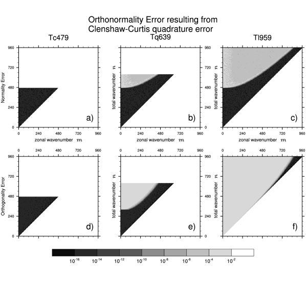
Figure 1: (a-c) Normality error (Eq. (23)) and (d-f) orthogonality error (Eq. (24)), evaluated using Clenshaw-Curtis quadrature, plotted as a function of the zonal wavenumber $m$ and the total wavenumber ($n$). The resolutions are (a,d): Tc479 ($N=479,J=959$), (b,e): Tq639 ($N=639,J=959$) and (c,f) Tl959 ($N=959,J=959$). Note the logarithmic scale in the colours.

4.2 Aliasing of quadratic and cubic terms evaluated on cubic Clenshaw-Curtis grids

Clenshaw-Curtis quadrature with cubic truncation does not guarantee alias-free spectral transforms for quadratic and cubic terms. As such, before applying Clenshaw-Curtis quadrature with cubic truncation to nonlinear models, we need to quantitatively assess the degree of aliasing for nonlinear terms. In this subsection we quantify aliasing errors for quadratic and cubic terms associated with spherical harmonics transforms and compare the Clenshaw-Curtis quadrature with cubic truncation and the Gaussian quadrature with linear truncation.

We quantify the aliasing errors by the following procedure. Consider the following series of operations:

1. Produce three scalar fields $U$, $V$, and $W$ on the sphere by randomly choosing their spectral representations $U_{n}^{m}$, $V_{n}^{m}$ and $W_{n}^{m}$. The spectral coefficients are chosen such that their $(m,n)$-component, $0\leq n\leq N_{\mathrm{trunc}}=479$, $|m|\leq n$, has both its real and imaginary part taken as an independent pseudo-random draw from a uniform distribution over $[1\times(n+1)^{-1/3},2\times(n+1)^{-1/3}]$.

2. Transform the scalar fields $U_{n}^{m},V_{n}^{m},W_{n}^{m}$ in spectral space into grid space by (1) to form $U(\lambda_{i},\phi_{j})$, $V(\lambda_{i},\phi_{j})$, $W(\lambda_{i},\phi_{j})$, and then compute, in grid space, quadratic and cubic terms $X_{q}(\lambda_{i},\phi_{j}):=U(\lambda_{i},\phi_{j})\times V(\lambda_{i},\phi_{j})$ and $X_{c}(\lambda_{i},\phi_{j}):=U(\lambda_{i},\phi_{j})\times V(\lambda_{i},\phi_{j})\times W(\lambda_{i},\phi_{j})$.

3. Finally transform the quadratic and cubic terms in grid space $X_{q}$ and $X_{c}$ back to spectral space by (5–6) to yield $X_{q,n}^{m}$ and $X_{c,n}^{m}$.

The scaling of the pseudo-random numbers by $(n+1)^{-1/3}$ in the step 1 is intended to mimic the power spectra of physical quantities typically encountered in geophysical applications (for instance, the power spectra of kinetic energy in three-dimensional turbulence in the inertial range follow $n^{-5/3}$-law, which corresponds to the spectral coefficients of divergence or vorticity being proportional to $\sim n^{-1/3}$). This choice is arbitrary and subjective, but we confirmed that it does not sensitively affect the conclusion by repeating the calculation changing the power from $-1/3$ to $-3,-2,-1,-1/2$ and 0.

We first perform the steps 1–3 on Tl1439 Gaussian grid ($N=1439,J=1440$) using Gaussian quadrature and a linear truncation at the total wavenumber of $N_{\mathrm{ref}}=1439(\approx 3N_{\mathrm{trunc}})$. This resolution is high enough to produce aliasing-free reference solutions of both quadratic and cubic terms, which we denote respectively by $X_{q,n}^{m,\mathrm{ref}}$ and $X_{c,n}^{m,\mathrm{ref}}$. We then repeat the steps 1–3 using the test resolutions and quadrature rules (Tl479 Gaussian or Tc479 Clenshaw-Curtis), using the same values of $U_{n}^{m}$, $V_{n}^{m}$ and $W_{n}^{m}$ as used to produce the reference solutions. The spectral coefficients of the quadratic and cubic terms computed with the test resolution and quadrature rule, denoted $X_{q,n}^{m,\mathrm{test}}$ and $X_{c,n}^{m,\mathrm{test}}$, are finally compared with the reference solutions $X_{q,n}^{m,\mathrm{ref}}$ and $X_{c,n}^{m,\mathrm{ref}}$ to define the normalised aliasing error for each pair of $(n,m)$:

$$\mathrm{AliasingErr}_{q,n}^{m} := {\left|X_{q,n}^{m,\mathrm{test}}-X_{q,n}^{m,\mathrm{ref}}\right|}/{\left|X_{q,n}^{m,\mathrm{ref}}\right|}$$ (25)

$$\mathrm{AliasingErr}_{c,n}^{m} := {\left|X_{c,n}^{m,\mathrm{test}}-X_{c,n}^{m,\mathrm{ref}}\right|}/{\left|X_{c,n}^{m,\mathrm{ref}}\right|}.$$ (26)

The results for Gaussian linear grid (Tl479; $N=479,J=480$) and Clenshaw-Curtis cubic grid (Tc479; $N=479,J=959$) are plotted in Figure 2. Clenshaw-Curtis quadrature performed on cubic grid (Figure 2, right panels) produces normalised aliasing errors below $10^{-5}$ (in the quadratic case, Figure 2b) or $10^{-8}$ (in the cubic case, Figure 2d) for most pairs of $(n,m)$ except in a small region with large $n/m$ ratio ($\gtrsim 10$). This is in contrast to the case of Gaussian quadrature performed on linear grid (Figure 2, left panel), where the normalised errors are almost anywhere greater than $10^{-4}$ (in the quadratic case, Figure 2a) or $10^{-3}$ (in the cubic case, Figure 2c), for some pairs of $(n,m)$ even exceeding $1$ in the quadratic case.

These results indicate that the aliasing errors that arise from the quadrature rule not being exact (as seen in Figure 2b,d) are orders of magnitude smaller than the aliasing errors that result from sub-sampling of waves in gridpoint space (as seen in Figure 2a,c); we elaborate on this in the next subsection. From this we may deduce that the aliasing from nonlinear terms in a model with Clenshaw-Curtis quadrature should remain under a controllable level as long as the quadrature is used with cubic truncation. This conclusion is further corroborated by the results of experiments shown in the next two sections.

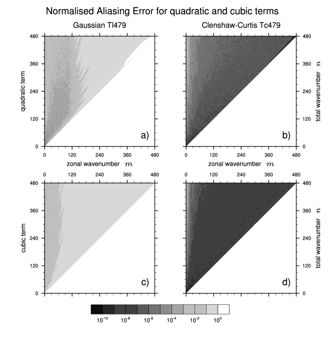
Figure 2: Normalised aliasing errors (see the text for definition) for (a,b) quadratic and (c,d) cubic terms evaluated with (a,c) Tl479 Gaussian quadrature with linear grid ($N=479,J=480$) and (b,d) Tc479 Clenshaw-Curtis quadrature with cubic grid ($N=479,J=959$). Note the logarithmic scale in the colours.

4.3 Explanation of small aliasing error following Trefethen (2008)

In Figures 1 and 2 we have observed that Clenshaw-Curtis quadrature gives fairly small errors even when the quadrature limit (17) is violated. This interesting feature can be understood from the mechanism discussed in section 5 of Trefethen (2008) which provides an intuitive and rigorous proof as to why the nominal factor-of-two advantage of Gaussian quadrature over Clenshaw-Curtis is rarely realised in practice. Trefethen’s argument is based on the version of Clenshaw-Curtis-type quadrature where the integrand function is expanded into $T_{l}(\cos\theta)$, the Chebyshev polynomials of the first kind; below we give a parallel discussion, expanding the integrand into $U_{l}(\cos\theta)$ instead of $T_{l}(\cos\theta)$.

On the Clenshaw-Curtis grid (13), it follows from the $2\pi$-periodicity of the sine function and its antisymmetry around 0, that, for any positive integer $p\leq J$, $U_{J+p}(\cos\theta)$ are indistinguishable (or aliased onto) $U_{J-p}(\cos\theta)$ (with the sign flipped):

$$U_{J+p}(\cos\theta_{j})=-U_{J-p}(\cos\theta_{j}),j=1,2,\cdots,J,$$ (27)

from which follows that $I_{J}^{CC}(U_{J+p})=-I_{J}^{CC}(U_{J-p})=-I(U_{J-p})=0$ (if $J\pm p$ is odd) or $-\frac{2}{J+1-p}$ (if $J\pm p$ is even), where $I(g):=\int_{-1}^{1}g(\cos\theta)d(\cos\theta)$ and $I_{J}^{CC}(g)$ denotes its approximation evaluated with $J$-point Clenshaw-Curtis quadrature rule (note that $I_{J}^{CC}(U_{J-p})$ is exact since $I_{J}^{CC}(\cdot)$ is exact for any polynomials with degrees at most $J-1$). Consequently the quadrature error for $U_{J+p}$ (which we denote by $e_{J}(p)$) is zero for odd $J+p$ and

$$e_{J}(p):=I(U_{J+p})-I_{J}^{CC}(U_{J+p})=\frac{2}{J+1+p}+\frac{2}{J+1-p}$$ (28)

for even $J+p$. Now, assuming that $J$ is odd (as is the case for a nestable grid), and expanding the integrand $g(\cos\theta)$ into $\sum_{l=0}^{\infty}a_{l}U_{l}(\cos\theta)$ which we assume to be uniformly converging, its quadrature error reads $a_{J+1}e_{J}(1)+a_{J+3}e_{J}(3)+a_{J+5}e_{J}(5)+\cdots$. Since $e_{J}(p)\sim O(J^{-1})$ for small $p$, and $a_{J+p}$ should rapidly decay as $p$ increases provided that $g(\cos\theta)$ is sufficiently smooth (which should be a valid assumption for most geophysical applications), the quadrature error for $g(\cos\theta)$ should be small if $J$ is large.

For example, with 959-point-Clenshaw-Curtis quadrature (Tc479 resolution), $U_{960}$ is integrated inexactly, but the error is only $e_{959}(1)=0.004$; errors for $U_{1200},U_{1440},U_{1680}$ and $U_{1920}$ are, respectively, 0.004, 0.005, 0.009 and 1.9. Errors for other polynomials are even smaller. For $T_{960},T_{1200},T_{1440},T_{1680}$ and $T_{1920}$, the errors are 0.002, 2e$-$6, 8e$-$6, 3e$-$5 and 2.0; similarly, for Legendre polynomials $P_{960},P_{1200},P_{1440},P_{1680}$ and $P_{1920}$ whose exact integrals are all zero, the errors are 8e$-$5, 4e$-$6, 5e$-$6, 1e$-$5 and 0.04. By contrast, with 479-point-Gaussian quadrature (Tl479 resolution), $U_{n},T_{n}$ or $P_{n}$ are all exactly evaluated up to $n=957$, but once the polynomial degree goes beyond the quadrature limit ($n\leq 2J-1$), the errors jump from zero to 3.1, 1.6 and 0.06, respectively, for $U_{958}$, $T_{958}$ and $P_{958}$.

5 Implementation to a shallow-water equation model

In implementing a new scheme, it is convenient to test it with a simpler model before introducing it to the full three-dimensional model. As a testbed, we first implemented Clenshaw-Curtis quadrature to a semi-Lagrangian shallow-water equations (SWE) model. The main focus of this paper is to examine the consistency between the models with Clenshaw-Curtis and Gaussian quadrature. Accordingly, the validations that follow are not designed to test the performance of the model itself but rather to detect any discrepancies arising from the use of different quadrature rules.

5.1 The model

The model used in this section is built by adapting the code of JMA-GSM. The governing equations are the advective form of the SWE on a rotating sphere described in section 2.2 of Williamson et al. (1992) but with the Coriolis terms incorporated in the left-hand side of the momentum equations as in Temperton (1997). The governing equations in advective form are then discretised in space and time by the Stable Extrapolation Two-Time-Level Semi-Lagrangian (SETTLS) method of Hortal (2002). The linear terms responsible for the fast gravity waves are treated semi-implicitly using the second-order decentering method described in Section 3.1.3 of Yukimoto et al. (2011). The semi-Lagrangian aspects of the scheme, such as finding of, and interpolation to, the departure points, are identical to the horizontal advection of JMA-GSM (Yukimoto et al., 2011; JMA, 2013). The reference state for the semi-implicit linearisation is the fluid at rest with a globally constant depth (5960 m for Williamson et al. (1992) test and 10 km for Galewsky et al. (2004) test). Other parameters are chosen to conform to the specifications in Williamson et al. (1992) and Galewsky et al. (2004) test cases. Throughout this section, and for all resolutions, the time step is chosen as $\Delta t=1200$ s.

The model may include numerical (hyper-)diffusion term in the governing equation:

$$\left(\frac{\partial X}{\partial t}\right)_{\mathrm{diffusion}}=-K\nabla^{2r}X$$ (29)

where $r$ is a positive integer. This is numerically solved implicitly in spectral space by applying the following operation at the end of each time step:

$$\left(X_{n}^{m}\right)_{\mathrm{after}}=\frac{1}{1+2K\Delta t\left\{\frac{n(n+1)}{a^{2}}\right\}^{r}}\left(X_{n}^{m}\right)_{\mathrm{before}}.$$ (30)

where $n$, $m$, $a$ and $\Delta t$ are, respectively, the total and zonal wavenumbers, the Earth’s radius and the time step.

We modify the model to allow an option to use Clenshaw-Curtis quadrature and compare the model runs produced with this option and the runs produced with the default Gaussian quadrature, under the framework of two standard test cases. The models with the two different quadrature rules run on different grids. To allow for accurate comparison, the Clenshaw-Curtis version of the model is adapted to output model states also on the Gaussian grids by converting the model state variables in spectral space to grid space using the inverse spherical harmonics transform (1) defined on the Gaussian grids. To ensure that the two versions start from exactly identical initial conditions, the initial conditions for the Clenshaw-Curtis version are produced by first computing them in grid space on the Gaussian grids, converting them to spectral space by the direct spherical harmonics transform (4) defined on the Gaussian grids, and then converting them back to grid space (but this time on the Clenshaw-Curtis grids) by the inverse spherical harmonics transform (1) defined on the Clenshaw-Curtis grids.

5.2 Test cases

The first test case examined is the evolution of the initially zonal flow over an isolated mountain proposed by Williamson et al. (1992) as Case #5. This test case is repeated for the resolutions of Tc31, Tc63, Tc127 and Tc255, both for Clenshaw-Curtis and Gaussian version of the model. No explicit numerical diffusion of the form (29) is used in any of the integrations for this case.

The solution of Williamson et al. (1992) test case #5 appears to be dominated by relatively low wavenumber components, so it may not be suitable for assessing model behaviour at higher wavenumbers. The second test case we examine, the barotropic jet instability test case proposed by Galewsky et al. (2004), allows us to assess the models in a more realistic, multi-scale flow situations. Galewsky et al. (2004) reported that weak explicit dissipation in the governing equations is necessary to obtain converged solutions, and suggested to apply harmonic diffusion ($r=1$ and $K=1.0\times 10^{5}~{}\mathrm{m}^{2}$ in (29)) to the governing equations to facilitate model comparison. We followed this suggestion and performed the test with a relatively high resolution of Tc479 ($\Delta x\sim$ 20 km at the Equator).

5.3 Results: flow over an isolated mountain

In interpreting the results, it should be noted that, unlike models with Eulerian advection scheme, exact agreement between Clenshaw-Curtis and Gaussian versions of the model is not expected in our semi-Lagrangian model since the two versions use different grids that result in differences in departure point interpolation. Nevertheless, we found, by plotting overlaid contour maps of relative vorticity (or any other) fields from the two versions of the model (not shown), that the two quadrature rules result in visually indistinguishable integrations up to at least 288 hours, for any of the tested resolutions. To quantitatively assess the difference, we computed the normalised $L_{2}$-differences defined as:

$$L_{2}\left(\xi^{CC},\xi^{G}\right):=\left(\frac{I\left(\xi^{CC}-\xi^{G}\right)}{I\left(\xi^{G}\right)}\right)^{1/2}$$ (31)

for zonal wind ($\xi=u$), meridional wind ($\xi=v$) and height field ($\xi=h$), for integration times $t$ from 0 to 288 hours at 6-hourly intervals. Here the superscripts $CC$ and $G$ represent the integration, respectively, by Clenshaw-Curtis and Gaussian versions of the model, and the the spherical integral $I(\xi)$ of the square of a variable $\xi$

$$I(\xi):=\frac{1}{4\pi}\int_{-\frac{\pi}{2}}^{\frac{\pi}{2}}\int_{0}^{2\pi}\xi(\lambda,\phi)^{2}d\lambda d\cos{\phi}d\phi$$ (32)

is numerically evaluated with Gaussian quadrature using $\xi^{CC}$ and $\xi^{G}$ both defined on the Gaussian grid.

The normalised $L_{2}$-differences of the zonal wind fields (Figure 3) are generally very small. They grow as the integration length gets longer but seem to saturate by $\sim$ 10-day integration. Higher resolutions result in smaller differences, presumably due to reduced interpolation errors in semi-Lagrangian advection. At saturation, the normalised differences are $\sim 10^{-3}$ with Tc31 resolution and $\sim 10^{-5}$ with Tc255 resolution, which are in practice negligibly small. Similar results were also observed for $v$ and $h$ fields (not shown).

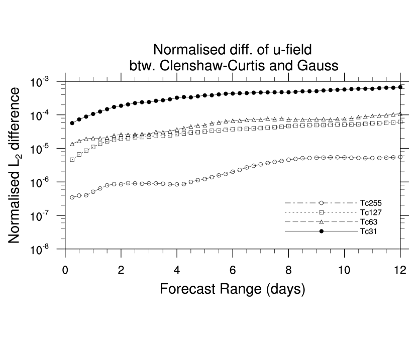
Figure 3: Normalised $L_{2}$-difference between Clenshaw-Curtis and Gaussian integration results for the zonal wind field plotted as a function of integration length. Note the log scale in the $y$-axis.

5.4 Results: Barotropic jet instability

With sharp frontal structures present in the solution, in the barotropic jet instability test, one may expect to see a larger discrepancy between the two versions of the model with different quadrature rules and the associated grids. We observed, however, that the two versions yielded results that are visually indistinguishable (Figure 4a), even at integration length as long as 144 hours (6 days) by which time multiple rolled-up vortical structures develop. The difference between the two can be found mainly in the frontal regions with strong vorticity gradients (Figure 4b), but the differences are smaller than the raw values by more than five orders of magnitude (note the different contour intervals in panels (a) and (b) of Figure 4). The normalised $L_{2}$-difference for any of $u,v$ and $h$ field (not shown) were below $10^{-7}$, again indicating that the discrepancies arising from use of different quadrature rules and the associated grids are negligible in practice.

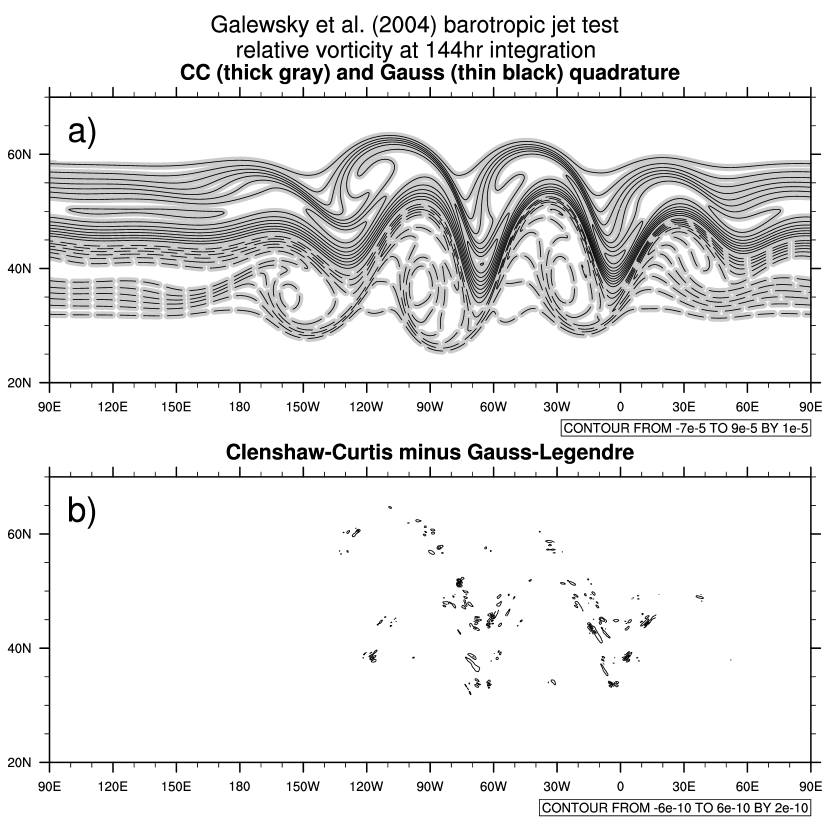
Figure 4: (a) Snapshot of relative vorticity field at day 6 from the barotropic jet instability test case produced with Clenshaw-Curtis (thick gray lines) and Gaussian (thin black lines) versions of the model at Tc479 ($\Delta x\sim 20$ km) resolution, and (b) the difference between the two. Contour intervals are $10^{-5}$ s in (a) and $2\times 10^{-10}$ s in (b). Positive and negative values are drawn, respectively, with solid and dashed contours, and the zero contours are omitted. Note that in (a) the two sets of contour lines are completely superimposed.

6 Implementation to a hydrostatic primitive equations model

6.1 The model

Clenshaw-Curtis quadrature is implemented to the dry dynamical core of JMA-GSM. It is an HPE model with Semi-Implicit Semi-Lagrangian (SISL) time discretisation. The horizontal discretisation is spectral with spherical harmonics as the basis functions, and the vertical discretisation employs finite differencing on $\sigma-p$ hybrid coordinate (Simmons and Burridge, 1981) with 100 layers extending from the surface up to 0.01 hPa. Detailed description of the model’s dynamical core can be found in Section 3.1 of Yukimoto et al. (2011) and Section 3.2.2 of JMA (2013).

As with most other SISL spectral models, by default JMA-GSM uses linear truncation. Since Clenshaw-Curtis quadrature requires cubic (or higher) grid truncation, in this study JMA-GSM is modified to allow for cubic truncation. All the results shown in this section are produced with Tc159 horizontal resolution ($\Delta x\sim 60$ km at the Equator) and a time step $\Delta t=1200$ s.

6.2 Test case specification

To assess any discrepancies in the forecasts that result from the use of Clenshaw-Curtis quadrature instead of the standard Gaussian quadrature, we perform the standardised test case proposed by Jablonowski and Williamson (2006) and adopted by numerous studies that implement new schemes to global atmospheric dynamical cores. The Jablonowski-Williamson test case comprises two parts. The first part, the steady-state test, initialises the model with an analytic, baroclinically-unstable steady-state solution to the HPE, and tests the model’s ability to maintain this steady-state initial condition. The second part, the baroclinic wave instability test, initialises the model with the same steady-sate solution but with a localised small-amplitude perturbation in the zonal wind field superimposed on the westerly jet axis located in the Northern Hemisphere mid-latitude. The small perturbation eventually develops into a train of unstable baroclinic waves that experiences nonlinear break-down by $\sim$ day 9. This second test allows us to examine the model’s behaviour in a situation akin to a typical mid-latitude synoptic condition with sharp fronts and fine-scale eddies.

6.3 Results

6.3.1 Steady-state test

We first examine the impact of quadrature choice on the model’s ability to maintain the steady-state solution by comparing, between the Clenshaw-Curtis and Gaussian versions of the model, the two measures of steady-state maintenance proposed by Jablonowski and Williamson (2006). The first measure, denoted as $l_{2}\left(u(t)-\bar{u}(t)\right)$ and defined as the square root of the three-dimensional integral of zonally asymmetric part of the zonal wind $u$ field (see Eq. (14) of Jablonowski and Williamson (2006)), quantifies to what extent the model is able to keep the zonally symmetric structure of the steady initial state. The second measure, denoted as $l_{2}\left(\bar{u}(t)-\bar{u}(t=0)\right)$ and defined as the square root of the three-dimensional integral of the departure of the zonal component $\bar{u}(t)$ of the zonal wind at time $t$ from that at the initial time (see Eq. (15) of Jablonowski and Williamson (2006)), complements the first measure and quantifies how much the zonal mean of $u$ field deviates from the initial zonally symmetric steady state over the course of integration.

As shown in Figure 5, the Clenshaw-Curtis and Gaussian versions of the model result in virtually identical $l_{2}$ error measures. The relative difference between the two versions of the model (defined as the difference normalised by the error of the Gaussian version; drawn with dotted lines and to be read on the right axis) is at most 2% for the first measure (Figure 5a) and is well below $\sim$1 % for the second measure (Figure 5b), indicating that the choice of the quadrature rule and the associated grid does not affect the model’s ability to maintain the steady-state initial condition.

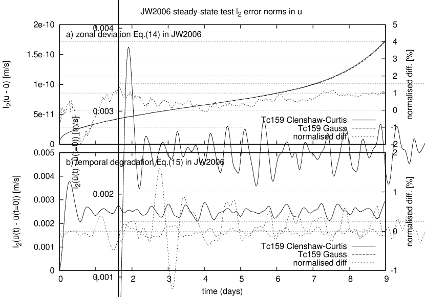
Figure 5: $l_{2}$ measures of steady-state maintenance in the steady-state test of Jablonowski and Williamson (2006) computed for (solid) Clenshaw-Curtis and (dashed) Gaussian versions of the dynamical core of JMA-GSM. (a) the zonal symmetry measure $l_{2}\left(u(t)-\bar{u}(t)\right)$. (b) the temporal degradation of the zonal mean zonal wind $l_{2}\left(\bar{u}(t)-\bar{u}(t=0)\right)$. Note that the solid and dashed lines are almost superposed both in (a) and (b). The dotted lines (to be read on the right axis) represent the relative difference between the Clenshaw-Curtis and Gaussian results normalised by the values of Gaussian results.

6.3.2 Baroclinic instability wave test

As in the barotropic jet instability test for SWE model (section 5.4, Figure 4), with sharp fronts present in the solution, we can expect the baroclinic instability wave test to better reveal discrepancies (if any) in the numerical results arising from the use of different quadrature rules and the associated grids. Just like in section 5.4, however, again we confirmed a high degree of agreement between the solutions from Clenshaw-Curtis and Gaussian versions of the model. As an example, we show the snapshots of 850 hPa temperature field at day-9 integration in Figure 6a. The results from Clenshaw-Curtis version (thick gray contours) and Gaussian version (thin black contours) are indistinguishable on this plot, and the difference between the two (Figure 6a) exhibit noisy patterns localised along the fronts and with very small amplitude (at most 0.13 K), indicating that no systematic difference results from the use of different quadrature rules.

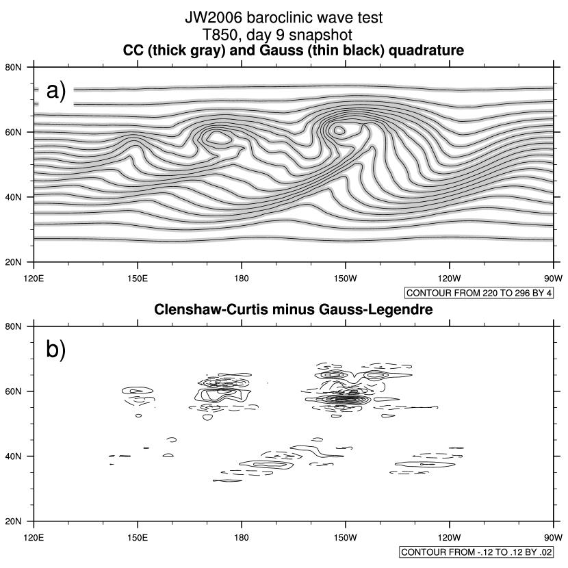
Figure 6: (a) Snapshot of 850-hPa temperature at day 9 from the baroclinic instability wave test case produced with Clenshaw-Curtis (thick gray lines) and Gaussian (thin black lines) versions of JMA-GSM dynamical core run at Tc159 resolution, and (b) the difference between the two. Contour intervals are 4 K in (a) and 0.02 K in (b). In (b), positive and negative values are drawn, respectively, with solid and dashed contours, and the zero contours are omitted. Note that in (a) the two sets of contour lines are completely superimposed.

7 Conclusion and future directions

Traditional global spectral atmospheric models adopt Gaussian quadrature, and the non-nested property of its associated irregular latitudinal quadrature nodes (the Gaussian grid) makes it difficult if not impracticable to apply multigrid approaches to global spectral models. To facilitate straightforward use of a multigrid method in a global spectral model in the future, in this study we proposed to adopt Clenshaw-Curtis quadrature in evaluating direct (grid-to-wave) Legendre transform. With Clenshaw-Curtis quadrature, the latitudinal grids (or quadrature nodes) are equispaced, so that the model grid for an arbitrary horizontal resolution includes the model grid for half its horizontal resolution as its complete subset, allowing for implementation of a multigrid method without a need for any off-grid interpolation.

Theoretical consideration shows, and numerical computation demonstrated, that Clenshaw-Curtis quadrature guarantees exact (up to machine precision) spherical harmonics transforms if it is used with cubic (or higher-order) grid truncation. One may argue that having to move from linear or quadratic truncation, which are the norm for the current semi-Lagrangian or Eulerian spectral models, respectively, is a serious limitation, but that is not the case for high-resolution modelling since, as shown by recent studies at ECMWF (Wedi, 2014), higher-order truncation is anyhow necessary to suppress aliasing errors and the resultant spectral blocking at a resolution as high as $\Delta x<$ 10 km.

Comparison of the Clenshaw-Curtis and Gaussian versions of the shallow-water model and dry hydrostatic primitive equations model, both with cubic grid and with semi-Lagrangian advection scheme, performed under the framework of idealised standard test cases, demonstrated that Clenshaw-Curtis quadrature gives model predictions that are almost identical to those obtained with the standard Gaussian quadrature.

Our ultimate goal is to ensure computational efficiency of a global spectral non-hydrostatic atmospheric model by enabling a multigrid approach, as outlined in Appendix C, and this study serves as a first step in this direction. The success (or not) of such an approach is not clear, particularly because the future evolution of the high-performance computing (HPC) architecture is still in a state of flux. It has long been predicted that spectral models will face a serious challenge on a massively parallel architecture because their current algorithms require global inter-node communications on every time step. To maintain admissible scalability on future architectures, therefore, global models would have to abandon, or at least reduce reliance on, spectral transforms. In this line, ECMWF has recently introduced a structured grid system, called ‘cubic octahedral reduced Gaussian grid’ that assures exact spectral transforms via Gaussian quadrature (Malardel et al., 2016) while at the same time allowing for straightforward grid-based discretisation of horizontal derivatives that only requires neighbouring-node communications (Smolarkiewicz et al., 2016), whereby paving a path for a smooth transition from spectral to grid-based modelling (or hybridisation of the two methods). Their approach of allowing both spectral and grid-based discretisations on a single grid system is ingenious and appealing, and we assert that Clenshaw-Curtis quadrature, with its equispaced latitude grids, can be combined to yield cubic octahedral Clenshaw-Curtis grid (Figure 7a).

Compared to the Gaussian octahedral grid, the Clenshaw-Curtis octahedral grid has the advantage of allowing for a straightforward use of multigrid in gridpoint-space solution of elliptic equations that result from a (semi-)implicit time stepping. Moreover, it covers the globe entirely with triangular meshes (Figure 7a), unlike the Gaussian counterpart which has rectangular cells along the Equator. Its latitudinally-uniform grid spacing may also help to make the derivative stencils somewhat simpler.

Alternative grid alignments based on reduced Clenshaw-Curtis grid are also possible that cover the globe with triangular meshes. Figure 7b shows one such possibility, which may be called cubic icositetrahedral (24-face polyhedral) Clenshaw-Curtis grid, where the globe is divided into 24 triangular panels of equal area, 6 covering the Northern Hemisphere extratropics (from 90°N down to 30°N), 12 covering the tropical 30°N–30°S belt, and the remaining 6 covering the rest (from 90°S up to 30°S). Compared to the octahedral grid, having to shift the phase in zonal Fourier transforms in the tropical belt introduces additional complexity in the code, but the icositetrahedral grid gives more uniform grid spacing across latitudes and is more compatible (Figure 8) with the grid reduction rule of Miyamoto (2006) which guarantees numerically exact spherical harmonics transform by requiring, for each latitude $\phi_{j}$, that there be at least $4M_{j}+1$ longitudinal points (with cubic truncation) where $M_{j}$ is defined as the smallest zonal wavenumber for which $\left|\tilde{P}_{n}^{m}\left(\sin\phi_{j}\right)\right|<10^{-16}$ ($\sim$ double precision machine epsilon) holds for any $0\leq n\leq N$ and $|m|\leq M_{j}$. The effectiveness in terms of accuracy, computational efficiency on a massively parallel machine architecture, and ease of transition from the current spectral model, of using octahedral and/or icositetrahedral Clenshaw-Curtis grids, along with gridpoint-space-based multigrid methods, will be explored in our future project.

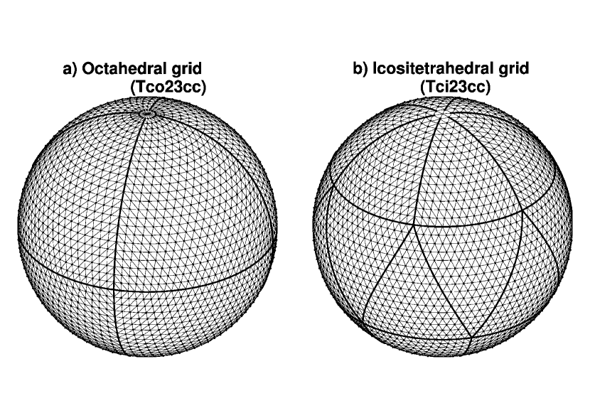
Figure 7: Cubic Clenshaw-Curtis (a) octahedral and (b) icositetrahedral grid for Tc23 resolution (which corresponds to 3.75°grid spacing in the meridional direction).

Figure 8: The number of gridpoints on each latitude circle for Tc255 resolution decided by (solid line) the grid reduction rule proposed by Miyamoto (2006) (see the text for detail), (dashed line) octahedral grid alignment, and (dotted line) icositetrahedral grid alignment.

Appendix A: Derivation of the Clenshaw-Curtis quadrature weights $w^{CC}_{j}$

Let $g(\cos\theta)$ be the integrand as defined in (12) and assume that $g(\cos\theta)$ can be expanded by the Chebyshev polynomials of the second kind of degrees up to $J-1$, giving

$$g(\cos\theta)\sin\theta=\sum_{l=0}^{J-1}a_{l}U_{l}\left(\cos\theta\right)\sin\theta=\sum_{p=1}^{J}a_{p-1}\sin{p\theta}$$ (A1)

The FFT-based derivation of the quadrature obtains the expansion coefficients $a_{l}$ by performing DST on $g(\cos{\theta})\sin\theta$ and then analytically integrates each summand in the rightmost-hand side of (A1). The alternative derivation by Boyd (1987) expands $g(\cos\theta)\sin\theta$ into a linear combination of “trigonometric cardinal functions” $\left\{C_{j}(\theta)\right\}_{j=1}^{J}$ rather than the sine series:

$$g(\cos\theta)\sin\theta=\sum_{j=1}^{J}\left\{g(\cos\theta_{j})\sin\theta_{j}\right\}C_{j}(\theta)$$ (A2)

where $\left\{C_{j}(\theta)\right\}_{j=1}^{J}$ are the transformed basis of the space spanned by the sine series $\left\{\sin{p\theta}\right\}_{p=1}^{J}$ that satisfies

$$C_{j}(\theta_{i})=\delta_{ij}$$ (A3)

for any $i,j\in\left\{1,2,\cdots,J\right\}$ with the nodes $\theta_{j}$ chosen as in (13). As shown in the Appendix of Boyd (1987), by exploiting the discrete orthonormality of $\left\{\sin{p\theta}\right\}_{p=1}^{J}$ on the points in (13), the cardinal functions $C_{j}(\theta)$ can be expressed as

$$C_{j}(\theta) = \frac{2}{J+1}\sum_{p=1}^{J}\sin{p\theta_{j}}\sin{p\theta}.$$ (A4)

The explicit expression of the quadrature weights $w^{CC}_{j}$ as shown in (16) follows from plugging (A4) into (A2) and then carrying out the integration from $\theta=0$ to $\theta=\pi$. $\blacksquare$

Appendix B: A comment on parity exploitation in spherical harmonics transforms

The associated Legendre functions $\tilde{P}_{n}^{m}(\sin\phi)$ are all either symmetric (if $n\equiv m\mod 2$) or antisymmetric (otherwise) across the Equator. This parity property, along with the hemispheric symmetry of the Gaussian latitudes and the Gaussian weights $w^{G}_{j}$, can be exploited to halve the computational cost of preparing $\tilde{P}_{n}^{m}(\sin\phi_{j})$ and $w^{G}_{j}$ (since they are only necessary for $j\leq J/2$) and of performing direct or inverse associated Legendre transforms, while at the same time preserving the hemispheric symmetry of the solutions. For example, the direct transform (9) can be rewritten as

$$X_{n}^{m}=\sum_{j=1}^{J/2}X^{m}_{S}(\phi_{j})\tilde{P}_{n}^{m}(\sin\phi_{j})w^{G}_{j}\quad n\equiv m\mod 2$$ (B1)

$$X_{n}^{m}=\sum_{j=1}^{J/2}X^{m}_{A}(\phi_{j})\tilde{P}_{n}^{m}(\sin\phi_{j})w^{G}_{j}\quad n\not\equiv m\mod 2$$ (B2)

where the decomposition of $X^{m}(\phi_{j}),j=1,\cdots,J$ into its symmetric and antisymmetric components $X^{m}_{S}(\phi_{j}):=X^{m}(\phi_{j})+X^{m}(\phi_{J+1-j})$ and $X^{m}_{A}(\phi_{j}):=X^{m}(\phi_{j})-X^{m}(\phi_{J+1-j}),j=1,\cdots,J/2$, which takes only $O(J)$ operations, is assumed to be performed prior to the transform. The inverse transform (2) can be similarly economised.

The same technique can be readily applied to the Clenshaw-Curtis version of the associated Legendre transforms because, as in the Gaussian case, Clenshaw-Curtis latitudes and weights are symmetric across the Equator. The only caveat to note here is that, unlike the Gaussian, Clenshaw-Curtis latitudes include the Equator, resulting in odd numbers of latitudinal gridpoints in total. Hence, the parity-exploited version of the direct transform becomes:

$$X_{n}^{m}=\sum_{j=1}^{(J+1)/2}X^{m}_{S}(\phi_{j})\tilde{P}_{n}^{m}(\sin\phi_{j})w^{CC}_{j}\quad n\equiv m\mod 2$$ (B3)

$$X_{n}^{m}=\sum_{j=1}^{(J+1)/2}X^{m}_{A}(\phi_{j})\tilde{P}_{n}^{m}(\sin\phi_{j})w^{CC}_{j}\quad n\not\equiv m\mod 2$$ (B4)

where $X^{m}_{S}(\phi_{j})$ and $X^{m}_{A}(\phi_{j})$ are defined as in (B1,B2) except for $X^{m}_{S}(\phi_{(J+1)/2}):=X^{m}(\phi_{(J+1)/2})$ and $X^{m}_{A}(\phi_{(J+1)/2}):=0$, and likewise for the inverse transform.

As stated above, parity exploitation not only saves computational costs but also helps to preserve the symmetry of solutions over the two hemispheres. This can be confirmed, for instance, by meridionally flipping the initial condition, running the model, and then meridionally flipping the solution again and checking if the solutions with and without flipping operations agree with each other. We have confirmed that this holds for our implementation using the Galewsky test described in section 5.4 (not shown).

Appendix C: Sketch on how Clenshaw-Curtis quadrature and grid will simplify multigrid implementation

To clarify the motivation behind introducing the nestable Clenshaw-Curtis grid in a global spectral atmospheric model, in this appendix we briefly describe how the proposed grid and quadrature will help to implement multigrid methods in a global spectral atmospheric model. Readers unfamiliar with multigrid nomenclature are invited to refer to, for example, the review by Fulton et al. (1986). Actually implementing multigrid methods to a global spectral model is beyond the scope of this paper and is planned to be addressed in our future work.

Let us denote the governing equations of the non-hydrostatic atmospheric dynamics symbolically as

$$\frac{DX}{Dt}=\mathcal{M}(X)$$ (C1)

where $X$ is the state vector and $\mathcal{M}$ is the nonlinear tendency operator. As discussed in Bénard (2004), there are two semi-implicit approaches, both iterative, to stably integrate C1) with a long time step.

In the first, non-constant-coefficient SISL approach, we divide $\mathcal{M}(X)$ into slow and fast components

$$\mathcal{M}(X)=\mathcal{M}^{\mathrm{slow}}(X)+\mathcal{M}^{\mathrm{fast}}(X)$$ (C2)

and the fast part $\mathcal{M}^{\mathrm{fast}}(X)$ is further partitioned into its tangent-linearisation $\mathcal{L^{*}}(X-X^{*})$ around some reference state $X^{*}$ and the residual $\mathcal{M}^{\mathrm{fast}}(X)-\mathcal{L^{*}}(X-X^{*})$, yielding:

$$\frac{DX}{Dt}=\mathcal{N}(X)+\mathcal{L^{*}}{X},$$ (C3)

where the operator $\mathcal{N}$ is defined so that (C1) combined with (C2) matches (C3), which is then descretised in time to give

$$\frac{X_{A}^{+}-X_{D}^{0}}{\Delta t}=\overline{\mathcal{N}(X)}^{(+1/2)}+\frac{1}{2}\left(\mathcal{L^{*}}{X_{A}^{+}}+\mathcal{L^{*}}{X_{D}^{0}}\right)$$ (C4)

where subscripts $A$ and $D$ denote values at the arrival and departure points, respectively, superscripts $+$ and $0$ denote values at the future and current time steps, respectively, and the overline $\overline{(\cdot)}$with superscript $(+1/2)$ denotes mean over the trajectory from current time at departure point to future time at arrival point, approximated by some extrapolation scheme such as SETTLS (Hortal, 2002) using the past and the current time step. Arranging all the unknown future state on the left hand side and all the known quantities on the right, (C4) results in the following linear systems of equations that can be arranged into a Helmholtz-type elliptic equation

$$\left(\mathcal{I}-\Delta t/2\mathcal{L^{*}}\right)X_{A}^{+}=F$$ (C5)

where $\mathcal{I}$ is the identity operator. In contrast to a hydrostatic system where choosing the reference state $X^{*}$ to be horizontally homogeneous, which renders (C5) a constant-coefficient elliptic equation that can be efficiently solved in spectral space, allows sufficient stability, non-hydrostatic dynamics requires the reference state $X^{*}$ to be inhomogeneous to bring $\mathcal{L^{*}}$ closer to $\mathcal{M}^{\mathrm{fast}}$ to achieve reasonable stability, rendering (C5) a non-constant-coefficient elliptic equation that needs to be solved iteratively.

An alternative, ‘more implicit’ approach stabilises the integration by approximately solving the fully implicit time discretisation of (C1):

$$\frac{X_{A}^{+}-X_{D}^{0}}{\Delta t}=\frac{1}{2}\left(\mathcal{M}(X_{A}^{+})+\mathcal{M}(M_{D}^{0})\right)$$ (C6)

with some generic nonlinear elliptic solver or with an iterative centred-implicit (ICI) scheme (Bénard, 2004) that allows to exploit the spectral constant-coefficient semi-implicit solver.

Either approach results in iterative solution of a linear or nonlinear elliptic equation, for which multigrid is an effective approach. The nested property of Clenshaw-Curtis grid (section 3.2), while not necessarily reduces computational cost in terms of operation count, will allow an easier implementation (with less coding effort and possibly less inter-node communications) of multigrid operations than the non-nested Gaussian grid would require. Restriction (grid transfer from higher- to lower-resolution) and prolongation (from lower- to higher-resolution) in spectral space are trivial since the lower-resolution spectral space is a proper subset of the higher-resolution spectral space. Restriction in grid space can be achieved by simple injection (or thinning; skipping every other grid) thanks to the nested property; note that non-nested grid like the Gaussian would necessitate off-grid interpolation, requiring some extra coding effort and possibly additional inter-node communication in a parallelised environment. Restriction from the higher-resolution grid space to the lower-resolution spectral space can be economically performed by the mechanism discussed in section 3.2, unlike in the Gaussian case where a costly high-resolution forward transform would be necessary. Prolongation in grid space can be achieved cheaply and locally (i.e., without a need for inter-node communication) by simple linear or spline interpolation in situations where spectral accuracy is not desired.

Using the economical grid transfer operations discussed above as building blocks, any multigrid solvers should be able to be constructed straightforwardly. As an illustrative example, consider the simplest-possible multigrid scheme, a V-cycle with only two grids (with Tc479 finer grid and Tc239 coaser grid, for example) applied to solving the non-constant coefficient elliptic problem (C5). The algorithm proceeds as follows:

1. At Tc479 resolution, approximately solve (C5) by some elliptic solver, e.g., iterative relaxation or Krylov subspace scheme in grid space starting from, e.g., the spectrally computed solution of the constant-coefficient approximation of (C5), with the horizontal derivatives evaluated pseudo-spectrally. At this point iteration does not have to be repeated until convergence, but the high wavenumber components should reasonably converge. Denote the current approximation by $X_{1}^{\mathrm{Tc479}}$ and compute the residual $R^{\mathrm{Tc479}}:=(\mathcal{I}-\Delta t/2\mathcal{L^{*}})X_{1}^{\mathrm{Tc479}}-F$.

2. Restrict $R^{\mathrm{Tc479}}$ into Tc239 space to obtain $R^{\mathrm{Tc239}}$ and solve the residual equation $(\mathcal{I}-\Delta t/2\mathcal{L^{*}})Y=-R^{\mathrm{Tc239}}$ for $Y$. This can be done by the same method as in step 1. but at the lower resolution. The resultant $Y$ is a lower-resolution approximation to the error $X_{A}^{+}-X_{1}^{\mathrm{Tc479}}$.

3. Prolong $Y$ to Tc479 resolution, then add to $X_{1}^{\mathrm{Tc479}}$ to yield the improved approximate solution $X_{2}^{\mathrm{Tc479}}$, and repeat the relaxation as in step 1., starting from $X_{2}^{\mathrm{Tc479}}$ as the first guess, with a tighter convergence criterion to ensure further improved approximation.

The ‘more implicit’ solver that approximately solves (C6) should be similarly accelerated by a multigrid approach by using, e.g., the nonlinear multigrid full approximation scheme (FAS).

Finally, we postulate that employing the pseudo-spectral multigrid approach as outlined above will foster smooth and gradual transition from spectral modelling to grid-based (or grid/spector hybrid) modelling since, in the above-outlined framework, the grid-space representation of the horizontal derivatives evaluated by the pseudo-spectral method can be readily replaced by local horizontal derivatives evaluated by some grid-based scheme such as finite difference, finite volume, or finite/spectral element. Given that grid-based elliptic solvers tend to be less efficient at larger scale, a grid/spector hybrid approach, where a grid-based multigrid method with shallow layers is combined with a spectral elliptic solver used only at the coarsest grid with moderate resolution, seems a reasonable strategy that compromises the need to avoid global inter-node communications and to maintain acceptable accuracy and convergence rate.

References

- Adams and Swartztrauber (1997) Adams JC, Swartztrauber PN. 1997. SPHEREPACK 2.0: A model development facility. NCAR Tech. Note NCAR/TN-436-STR, 62 pp. DOI: 10.5065/D6Z899CF.
- Bénard (2004) Bénard P. 2004. ‘Aladin–NH/AROME dynamical core: status and possible extension to IFS’. InProc. ECMWF Seminar on Recent Developments in Numerical Methods for Atmosphere and Ocean Modelling, Reading (UK), 6–10 September 2004. pp 27–40.
- Bogaert (2014) Bogaert I. 2014. Iteration-free computation of Gauss–Legendre quadrature nodes and weights. SIAM J. Sci. Comput. 36: C1008–C1026.
- Boyd (1987) Boyd JP. 1987. Exponentially convergent Fourier-Chebshev quadrature schemes on bounded and infinite intervals. J. Sci. Comput. 2(2): 99–109.
- Cheong (2000) Cheong HB. 2000. Application of double Fourier series to the shallow-water equations on a sphere. J. Comp. Phys. 165: 261–287.
- Clenshaw and Curtis (1960) Clenshaw CW, Curtis AR. 1960. A method for numerical integration on an automatic computer. Numerische Mathematik. 2: 197–205.
- Enomoto (2015) Enomoto T. 2015. Comparison of computational methods of associated Legendre functions. SOLA. 11: 144–149. DOI: 10.2151/sola.2015-033
- Fejér (1933) Fejér L. 1933. Mechanische Quadraturen mit positiven Cotesschen Zahlen. Mathematische Zeitschrift. 37: 287–309.
- Fulton et al. (1986) Fulton SR, Ciesielski PE, Schubert WH. 1986. Multigrid methods for elliptic problems: a review. Mon. Wea. Rev. 114: 943–959.
- Galewsky et al. (2004) Galewsky J, Scott RK, Polvani LM. 2004. An initial-value problem for testing numerical models of the global shallow-water equations. Tellus. 56A: 429–440.
- Gentleman (1972a) Gentleman WM. 1972a. Implementing Clenshaw-Curtis quadrature. I. Comm. ACM. 15: 337–342.
- Gentleman (1972b) ——–. 1972b. Implementing Clenshaw-Curtis quadrature. II. Comm. ACM. 15: 343–346.
- Hale and Townsend (2013) Hale N, Townsend A. 2013. Fast and accurate computation of Gauss-Legendre and Gauss-Jacobi quadrature nodes and weights. SIAM J. Sci. Comput. 35: A652–A674.
- Heikes et al. (2013) Heikes PR, Randall DA,Konor CS. 2013. Optimized icosahedral grids: Performance of finite-difference operators and multigrid solver. Mon. Wea. Rev. 141: 4450–469. DOI: 10.1175/MWR-D-12-00236.1
- Hortal (2002) Hortal M. 2002. The development and testing of a new two-time-level semi-Lagrangian scheme (SETTLS) in the ECMWF forecast model. Q. J. R. Meteorol. Soc. 128: 1671–1687.
- Hoskins and Simmons (1975) Hoskins BJ, Simmons AJ. 1975. A multi-layer spectral model and the semi-implicit method. Q. J. R. Meteorol. Soc. 101: 637–655.
- Jablonowski and Williamson (2006) Jablonowski C, Williamson DL. 2006. A baroclinic instability test case for atmospheric model dynamical cores. Q. J. R. Meteorol. Soc. 132: 2943–2975.
- JMA (2013) JMA. 2013. Outline of the operational numerical weather prediction at the Japan Meteorological Agency (March 2013), Appendix to WMO Technical Progress Report on the Global Data-processing and Forecasting System (GDPFS) and Numerical Weather Prediction (NWP) Research, 188pp. Available online at http://www.jma.go.jp/jma/jma-eng/jma-center/nwp/outline2013-nwp/index.htm
- Jones (1999) Jones PW. 1999. First- and second-order conservative remapping schemes for grids in spherical coordinates. Mon. Wea. Rev. 127: 2204–2210.
- Juang (2004) Juang HMH. 2004. A reduced spectral transform for the NCEP Seasonal Forecast Global Spectral Atmospheric Model. Mon. Wea. Rev. 132: 1019–1035.
- Machenhauer and Daley (1972) Machenhauer B, Daley R. 1972. A baroclinic primitive equation model with a spectral representation in three dimensions. Report No. 4. Institute for Theoretical Meteorology, Copenhagen University. 63pp. DOI: 10.13140/RG.2.2.19144.32002.
- Malardel et al. (2016) Malardel S, Wedi N, Deconinck W, Diamantakis M, Kühnlein C, Mozdzynski G, Hamrud M, Smolarkiewicz P. 2016. A new grid for the IFS. ECMWF Newsletter. 146: 23–28.
- Miyamoto (2006) Miyamoto K. 2006. Introduction of the Reduced Gaussian Grid into the Operational Global NWP Model at JMA. CAS/JSC WGNE Res. Activ. Atmos. Oceanic Modell. 36:06.09–06.10.
- NIST (2016) NIST. 2016. Digital Library of Mathematical Functions. http://dlmf.nist.gov/, Release 1.0.13 of 2016-09-16. F. W. J. Olver, A. B. Olde Daalhuis, D. W. Lozier, B. I. Schneider, R. F. Boisvert, C. W. Clark, B. R. Miller, and B. V. Saunders, eds.
- Orszag (1970) Orszag SA. 1970. Transform method for calculation of vector coupled sums: Application to the spectral form of vorticity equation. J. Atmos. Sci. 27: 890–895.
- Ritchie (1988) Ritchie H. 1988. Application of the semi-Lagrangian method to a spectral model of the shallow water equations. Mon. Wea. Rev. 116(8): 1587–1598. DOI: 10.1175/1520-0493(1988)116<1587:AOTSLM>2.0.CO;2
- Sandbach et al. (2015) Sandbach S, Thuburn J, Vassilev D, Duda MG. 2015. A semi-implicit version of the MPAS-Atmosphere Dynamical Core. Mon. Wea. Rev. 143: 3838–3855. DOI: 10.1175/MWR-D-15-0059.1
- Simmons and Burridge (1981) Simmons AJ, Burridge M. 1981. An energy and angular-momentum conserving vertical finite-difference scheme and hybrid vertical coordinates. Mon. Wea. Rev. 109: 758–766.
- Smolarkiewicz et al. (2016) Smolarkiewicz PK, Deconinck W, Hamrud M, Kühnlein C, Mozdynski G, Szmelter J, Wedi NP. 2016. A finite-volume module for simulating global all-scale atmospheric flows, J. Comp. Phys. 314: 287–304. DOI: 10.1016/j.jcp.2016.03.015
- Swartztrauber (1979) Swarztrauber PN. 1979. On the spectral approximation of discrete scalar and vector functions on the sphere. SIAM J. Numer. Anal. 16(6): 934–949.
- Swartztrauber (2002) ——–. 2002. On computing the points and weights for Gauss-Leggendre quadrature. SIAM J. Sci. Comput. 24: 945-954.
- Temperton (1991) Temperton C. 1991. On scalar and vector transform methods for global spectral models. Mon. Wea. Rev. 119(5): 1303–1307.
- Temperton (1997) ——–. 1997. Treatment of the Coriolis terms in semi-Lagrangian spectral models. Atmos. Ocean. 35: sup1. 293–302. DOI: 10.1080/07055900.1997.9687353
- Townsend (2015) Townsend A. 2015. The race to compute high-order Gauss-Legendre quadrature. SIAM News 48(2). Available online at https://sinews.siam.org/Details-Page/the-race-to-compute-high-order-gausslegendre-quadrature
- Trefethen (2008) Trefethen LN. 2008. Is Gauss quadrature better than Clenshaw-Curtis?. SIAM Rev. 50: 67–87.
- Ullrich et al. (2009) Ulllrich PA, Lauritzen PH, Jablonowski C. Geometrically Exact Conservative Remapping (GECoRe): Regular latitude-longitude and cubed-sphere grids. Mon. Wea. Rev. bf 137(6): 1721–1741.
- Waldvogel (2006) Waldvogel J. 2006. Fast construction of the Fejér and Clenshaw-Curtis quadrature rules. J. BIT Numer. Math. 46(1): 195–202. DOI: 10.1007/s10543-006-0045-4
- Wedi (2014) Wedi NP. 2014. Increasing horizontal resolution in NWP and climate simulations – illusion or panacea? Phil. Trans. R. Soc. A. 372: 20130289. DOI: 10.1098/rsta.2013.0289
- Williamson et al. (1992) Williamson DL, Drake JB, Hack JJ, Jakob R, Swarztrauber PN. 1992. A standard test set for numerical approximation to the Shallow Water equations in spherical geometry. J. Comp. Phys. 102: 211–224.
- Yoshimura (2012) Yoshimura H. 2012. Development of a nonhydrostatic global spectral atmospheric model using double Fourier series. CAS/JSC WGNE Res. Activ. Atmos. Oceanic Modell. 42: 3.05–3.06.
- Yukimoto et al. (2011) Yukimoto S, Yoshimura H, Hosaka M, Sakami T, Tsujino H, Hirabara M, Tanaka TY, Deushi M, Obata A, Nakano H, Adachi Y, Shindo E, Yabu S, Ose T, Kitoh A. 2011. Meteorological Research Institute-Earth System Model Version 1 (MRI-ESM1)– Model Description–. Tech. Rep. of the Meteorol. Res. Inst. 64: 1–96. DOI: 10.11483/mritechrepo.64