Tool Supported Analysis of IoT

Abstract

The design of IoT systems could benefit from the combination of two different analyses. We perform a first analysis to approximate how data flow across the system components, while the second analysis checks their communication soundness. We show how the combination of these two analyses yields further benefits hardly achievable by separately using each of them. We exploit two independently developed tools for the analyses.

Firstly, we specify IoT systems in IoT-LySa, a simple specification language featuring asynchronous multicast communication of tuples. The values carried by the tuples are drawn from a term-algebra obtained by a parametric signature. The analysis of communication soundness is supported by ChorGram, a tool developed to verify the compatibility of communicating finite-state machines. In order to combine the analyses we implement an encoding of IoT-LySa processes into communicating machines. This encoding is not completely straightforward because IoT-LySa has multicast communications with data, while communication machines are based on point-to-point communications where only finitely many symbols can be exchanged. To highlight the benefits of our approach we appeal to a simple yet illustrative example.

1 Introduction

Software is hardly built anymore as a stand-alone application. Over the last decades, the rise of distributed and concurrent applications has determined a crucial entanglement between computation and communication [17]. This phenomenon increasingly makes adaptability, reconfigurability, and openness paramount requirements of software. Therefore, it is nowadays crucial for designers and software engineers to take into account both properties of computation and communication when developing systems.

The Internet of Things (IoT) is one of the most advanced technological frontiers of the combination of computation and communication. By definition, IoT systems are made of several components that interact within complex (cyber-)physical environments. This emerging technology provides the momentum for the creation of new societal and economical opportunities, as long as IoT systems become trustworthy. Indeed, the great disruptive innovation that IoT systems can offer comes with an equally great threat: it is extremely hard to guarantee correctness properties of those systems. In fact, the overall correctness becomes the resultant of that of communication and that of computation. In Bruce Schneier’s words:

«The Internet of Things is fundamentally changing how computers get incorporated into our lives. Through the sensors, we’re giving the Internet eyes and ears. Through the actuators, we’re giving the Internet hands and feet. Through the processing – mostly in the cloud – we’re giving the Internet a brain. Together, we’re creating an Internet that senses, thinks, and acts. This is the classic definition of a robot, and I contend that we’re building a world-sized robot without even realizing it.» [5]

These issues are particularly critical because of the apparently easy use of IoT technologies hides their not trivial design, that becomes evident only when something goes wrong, e.g. when privacy can be compromised. Among many others, a recent example is that of a smart doll  that allows children to access the Internet via speech recognition software, and to control the toy via an app. However, this smart technology enables an attacker to also access personal data.

In this paper, we consider a simple yet realistic scenario to illustrate how to verify properties of IoT systems that arise from this prominent mix of computation and communication. We advocate the combination of two different techniques for supporting verification. To analyse the “computational dimension” we appeal to a static analysis technique that allows us to check control and data flow properties of systems. The soundness of “communication dimension” is instead verified through a choreographic framework. More precisely, we combine the analysis defined on IoT-LySa [10, 9] (a specification language tailored to IoT) and the analysis of communication soundness based on communicating finite-state machines (CFSMs) and global graphs [15].

An IoT system is specified as a set of IoT-LySa components that communicate through an asynchronous multicast mechanism. The values communicated in the system are drawn from a term-algebra obtained by a parametric signature. The control flow analysis for IoT-LySa [10] over-approximates the values that can be assigned to the local variables of a component, as well as where these values originated. This analysis allows designers to spot potential mistakes on how data are handled by components. In addition, the analysis computes the messages that a node may receive, but not the order in which they arrive, and it is thus insufficient for establishing the communication soundness.

Communication soundness is therefore checked by mapping the components to CFSMs and using ChorGram [14], a tool developed to verify the compatibility of communicating finite-state machines [15]. The compatibility property checked by ChorGram is defined in [15] and it is a condition guaranteeing absence of deadlocks, message obliviousness (i.e. messages sent but not received) [6], and of unspecified reception (i.e. a component receiving unexpected messages). We show how ChorGram flags possible communication mistakes when the set of CFSMs is not compatible and allows the designer to determine where the problem arises. Differently from the control flow analysis, the one made with ChorGram is insensitive to the data exchanged through the messages.

The main contribution of this paper is showing that the control flow analysis and the analysis of communication soundness based on a choreographic framework complement each other, and that it is worthwhile combining them for formally verifying IoT systems.

Structure of the paper

After reviewing the choreographic framework and IoT-LySa (cf. Section 2), we describe our running example and model it in IoT-LySa (cf. Section 3). Section 3 also shows how the analysis of the IoT-LySa specification can lead to detecting mistakes in the computation and help in fixing the errors. Section 5 illustrates how to use ChorGram to analyse the communication behaviour of our running example. This analysis flags some unexpected misbehaviour and helps fixing the problem. In order to combine these analyses Section 4 describes an encoding of the IoT-LySa systems into communicating machines. This encoding is not straightforward because IoT-LySa features multicast communications with data while communication machines are based on point-to-point communications where only finitely many symbols can be exchanged. Technical details are given in the appendices. Our concluding remarks are in Section 6.

2 Background

2.1 A choreographic framework for distributed systems

Choreographies advocate the so-called local and global views for specifying the behaviour of a system. In the first, one specifies the asynchronous communication behaviour of each component “in isolation”, while the interactions among the system components are seen as atomic actions that abstract away from asynchrony. Using a simple example, we will review the key ingredients of the local and global views adopted here, namely communicating finite-state machines [12] and (a variant of) global graphs [13].

Local view

Communicating finite-state machines (CFSMs) are a conceptually simple model for the analysis of communication protocols. A CFSM is basically a finite-state automaton with transitions that represent send or receive actions. Each machine is uniquely identified by a name and we use $\mathsf{\color[rgb]{0,0,1}{{A}}}$, ${\mathsf{\color[rgb]{0,0,1}{{B}}}}$, etc. to range over identifiers of CFSMs. A system consists of finitely many CFSMs that share unbounded FIFO channels to exchange messages. More precisely, for each pair $\mathsf{\color[rgb]{0,0,1}{{A}}}$ and ${\mathsf{\color[rgb]{0,0,1}{{B}}}}$ of CFSMs there is a channel from $\mathsf{\color[rgb]{0,0,1}{{A}}}$ to ${\mathsf{\color[rgb]{0,0,1}{{B}}}}$ (dubbed $\mathsf{}\cdot\mathsf{}$) and a channel in the other direction (dubbed $\mathsf{{\mathsf{\color[rgb]{0,0,1}{{B}}}}}\cdot\mathsf{\mathsf{\color[rgb]{0,0,1}{{A}}}}$). The use of buffers realises an asynchronous semantics: senders simply deposit messages in buffers without synchronising with receivers.

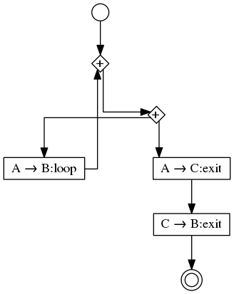
(a) Example of a system of CFSMs	(b) Global graph

Figure 1: A choreographic model

We illustrate the semantics of CFSMs by considering the system of three machines $\mathsf{\color[rgb]{0,0,1}{{A}}}$, ${\mathsf{\color[rgb]{0,0,1}{{B}}}}$, and $\mathsf{\color[rgb]{0,0,1}{{C}}}$ in Figure 1(a). Machine $\mathsf{\color[rgb]{0,0,1}{{A}}}$ repeatedly sends message $\mathsf{loop}$ to machine ${\mathsf{\color[rgb]{0,0,1}{{B}}}}$ until message $\mathsf{exit}$ is sent to machine $\mathsf{\color[rgb]{0,0,1}{{C}}}$. Machine ${\mathsf{\color[rgb]{0,0,1}{{B}}}}$ will consume any message sent by $\mathsf{\color[rgb]{0,0,1}{{A}}}$ and then wait for a message $\mathsf{exit}$ in the buffer $\mathsf{\mathsf{\color[rgb]{0,0,1}{{A}}}C}]\cdot\mathsf{{\mathsf{\color[rgb]{0,0,1}{{B}}}}}$ from $\mathsf{\color[rgb]{0,0,1}{{C}}}$. Finally, $\mathsf{\color[rgb]{0,0,1}{{C}}}$ forwards message $\mathsf{exit}$ to ${\mathsf{\color[rgb]{0,0,1}{{B}}}}$ once it has received it from $\mathsf{\color[rgb]{0,0,1}{{A}}}$. The configuration of a system is a snapshot that records the states in which each machine is in, and the contents of each channel. Initially, all CFSMs are in their initial states and buffers are empty. When, in the current configuration, a machine is in a state with an outgoing output transition, labelled say by $\mathsf{\mathsf{\color[rgb]{0,0,1}{{A}}}}\cdot\mathsf{{\mathsf{\color[rgb]{0,0,1}{{B}}}}}!{}{}$, then the output transition can be fired and move the machine $\mathsf{\color[rgb]{0,0,1}{{A}}}$ to the target state of the transition. At the same time the message $\mathsf{m}$ is deposited in the buffer $\mathsf{}\cdot\mathsf{}$. Similarly, if the machine is in a state with an outgoing input transition, labelled say by $\mathsf{\mathsf{\color[rgb]{0,0,1}{{A}}}}\cdot\mathsf{{\mathsf{\color[rgb]{0,0,1}{{B}}}}}?{}{}$, and the head of the buffer contains message $\mathsf{m}$ then the input transition can be fired removing $\mathsf{m}$ from the buffer and moving the machine to the target state of the transition. For instance, the system of our example in Figure 1(a) can reach the following configuration (from its initial one)

$$\langle\mathsf{\color[rgb]{0,0,1}{{A}}}:q,{\mathsf{\color[rgb]{0,0,1}{{B}}}}:q_{0},\mathsf{\color[rgb]{0,0,1}{{C}}}:q_{0}\ \ ;\ \ \mathsf{}\cdot\mathsf{}:[\mathsf{loop},\ldots,\mathsf{loop}],\mathsf{A}\cdot\mathsf{\mathsf{\color[rgb]{0,0,1}{{A}}}C}]:[\mathsf{exit}],\mathsf{\mathsf{\color[rgb]{0,0,1}{{A}}}C}]\cdot\mathsf{B}:[],\ldots\rangle$$

where (i) $\mathsf{\color[rgb]{0,0,1}{{A}}}$ is in state $q$ while machines ${\mathsf{\color[rgb]{0,0,1}{{B}}}}$ and $\mathsf{\color[rgb]{0,0,1}{{C}}}$ are in state $q_{0}$ and (ii) the buffer $\mathsf{}\cdot\mathsf{}$ contains a number of $\mathsf{loop}$ messages, the buffer $\mathsf{A}\cdot\mathsf{\mathsf{\color[rgb]{0,0,1}{{A}}}C}]$ contains the message $\mathsf{exit}$, and all the remaining buffers are empty. For simplicity, suppose that $\mathsf{\color[rgb]{0,0,1}{{A}}}$ sends only one $\mathsf{loop}$ message and then an $\mathsf{exit}$ message. In this configuration, both ${\mathsf{\color[rgb]{0,0,1}{{B}}}}$ and $\mathsf{\color[rgb]{0,0,1}{{C}}}$ can consume the message in their queues from $\mathsf{\color[rgb]{0,0,1}{{A}}}$; if the input of $\mathsf{\color[rgb]{0,0,1}{{C}}}$ is fired then the system reaches the configuration

$$\langle\mathsf{\color[rgb]{0,0,1}{{A}}}:q,{\mathsf{\color[rgb]{0,0,1}{{B}}}}:q_{0},\mathsf{\color[rgb]{0,0,1}{{C}}}:q\ \ ;\ \ \mathsf{}\cdot\mathsf{}:[\mathsf{loop}],\mathsf{A}\cdot\mathsf{\mathsf{\color[rgb]{0,0,1}{{A}}}C}]:[],\mathsf{\mathsf{\color[rgb]{0,0,1}{{A}}}C}]\cdot\mathsf{B}:[],\ldots\rangle$$

from where both the input of $\mathsf{loop}$ of ${\mathsf{\color[rgb]{0,0,1}{{B}}}}$ and the output from state $q$ of $\mathsf{\color[rgb]{0,0,1}{{C}}}$ are enabled and can be non-deterministically fired. Observe that the computation where $\mathsf{\color[rgb]{0,0,1}{{A}}}$ never sends message $\mathsf{exit}$ is possible; this will make $\mathsf{\color[rgb]{0,0,1}{{A}}}$ and ${\mathsf{\color[rgb]{0,0,1}{{B}}}}$ interact forever, while $\mathsf{\color[rgb]{0,0,1}{{C}}}$ will be waiting.

Global view

A global graph yields the description of the distributed work-flow of components exchanging messages. We borrow global graphs from [15] to formalise the global views of choreographies; an example of these graphs is in Figure 1(b). The nodes of a global graph are labelled by (resp ) to mark the starting (resp. termination) point of the choreography; by $\mathsf{\color[rgb]{0,0,1}{{A}}}\to{\mathsf{\color[rgb]{0,0,1}{{B}}}}:\mathsf{m}$ to indicate that participant $\mathsf{\color[rgb]{0,0,1}{{A}}}$ and ${\mathsf{\color[rgb]{0,0,1}{{B}}}}$ exchange message $\mathsf{m}$ ($\mathsf{\color[rgb]{0,0,1}{{A}}}$ being the sender and ${\mathsf{\color[rgb]{0,0,1}{{B}}}}$ the receivers); by to indicate either a choice, merge, or the entry-point of an iteration; or by to indicate either the start or the end of concurrent interactions. For example, the starting point of the global graph in Figure 1(b) is followed by the entry point of an iteration; the body of the iteration is a choice between two branches: in the left-most branch $\mathsf{\color[rgb]{0,0,1}{{A}}}$ and ${\mathsf{\color[rgb]{0,0,1}{{B}}}}$ exchange the message $\mathsf{loop}$ and go back to the entry point of the iteration; in the right-most branch $\mathsf{\color[rgb]{0,0,1}{{A}}}$ and $\mathsf{\color[rgb]{0,0,1}{{C}}}$ exchange the message $\mathsf{exit}$ followed by an exchange of the same message between $\mathsf{\color[rgb]{0,0,1}{{C}}}$ and ${\mathsf{\color[rgb]{0,0,1}{{B}}}}$, followed by a sink node where no further interactions happen.

An intuition of the semantics of a global graph can be given in terms of a “token game” similar to the one of Petri nets. The token starts from the initial node and follows the arcs of the graph; when the node reaches a choice node it continues along one branch; when the node reaches a fork node , new tokens start to flow along all the arcs and, dually, when all the tokens of the incoming arcs of a join gate are present then one token continues along the outgoing arc of the gate. For example, in our global graph, after the start, the machines either engage in an iteration where $\mathsf{\color[rgb]{0,0,1}{{A}}}$ and ${\mathsf{\color[rgb]{0,0,1}{{B}}}}$ exchange $\mathsf{loop}$ or $\mathsf{\color[rgb]{0,0,1}{{A}}}$ sends the message $\mathsf{exit}$ to $\mathsf{\color[rgb]{0,0,1}{{C}}}$, which in turn forwards it to ${\mathsf{\color[rgb]{0,0,1}{{B}}}}$ after which the protocol terminates.

In this paper, we will use ChorGram [14] a toolkit, based on the results of [15], that allows to reconstruct a global graph out of a system of CFSMs. In fact, ChorGram generates the presented global graph starting from the machines $\mathsf{\color[rgb]{0,0,1}{{A}}}$, ${\mathsf{\color[rgb]{0,0,1}{{B}}}}$, and $\mathsf{\color[rgb]{0,0,1}{{C}}}$ above.

As said above, systems of CFSMs evolve by moving from one configuration to another. If communication misbehaviours happen then “bad” configurations may be reached. A machine is in a sending (resp. receiving) state if all its outgoing transitions are send (resp. receive) actions. A state without any outgoing transition is said to be final. A state that is neither final, nor sending nor receiving is a mixed state. A system of CFSMs is communication sound if none of its reachable configurations is a deadlock and it is not message oblivious [6], where

• a configuration is a deadlock if all the buffers are empty, there is at least one machine in a receiving state, and all the other machines are either in a receiving state or in a final state;

• a system is not message oblivious [6] if whenever a message has been sent by a participant, that message will be eventually received.

Since CFSMs are Turing-complete, communication soundness is not decidable. However, systems enjoying the generalised multiparty compatibility (GMC) [15] are guaranteed to be sound and GMC is a decidable property supported by the ChorGram toolkit [16]. We will give an intuition of the GMC property in Section 5.

2.2 An overview of IoT-LySa

The language

We review IoT-LySa [10, 9], a specification language recently proposed for designing IoT systems. IoT-LySa is based on a process calculus and it has a specific focus on data collecting, aggregation, and communication. Indeed, by using IoT-LySa primitives designers can model the structure of a system and the interactions among the smart objects it is made of. A smart object is represented by a node that specifies multiple processes interacting through a shared local store, as well as sensors and actuators. In IoT-LySa store accesses are assumed as atomic. The processes are in charge of detailing how data are to be processed and exchanged among the nodes. A sensor of a node $\ell$ is an active entity that reads data from the physical environment at its own fixed rate, and deposits them in the local store of $\ell$. Actuators instead are passive: they just wait for a command to become active and operate on the environment. The current version of IoT-LySa is specifically designed to model monitoring system typical of smart cities, factories or farms. In this scenario, smart objects never leave their locations, while mobile entities, such as cars or people, carry no smart device and can only trigger sensors.

Communications in IoT systems often occur in a disciplined broadcasting manner. For that, IoT-LySa features a simple multicast communication among nodes. For example, the output of the first thermometer node Th₁ at line 25 in Figure 3

snd (temp,mt) to [Th,Th₂]

specifies that the message (temp,mt) has to be sent to two nodes, namely the thermostat Th and the second thermometer Th₂ (we will come back on this example in Section 3). The reception of a message is also done in a disciplined way: the receiver filters the messages flowing in the ether and only accepts some of them according to a sort of guard, following [8]. For example, consider the input of the thermostat node Th in Figure 2 at line 7

recv(temp;x)

The message described above passes the check, because what is at the left of the “;” in the payload, namely the guard temp, matches with the first element of the message sent. Then the value stored in mt is assigned to the variable x, as usual. If the guard is not passed, Th simply ignores the message. (Of course, the above extends to tuples of guards and of binding values.) This filtering input enables us to explicitly implement external choices, through the switch primitive. It was not originally included in [10, 9] although the construct can be encoded there.

We now intuitively describe other elements of IoT-LySa on the snippet of code in Figure 2. As done already, for readability, in this paper we are using a sugared syntax, from which the original IoT-LySa code can be easily extracted (see Appendix A). The thermostat node Th we are considering has no sensors and a single actuator ACon_off. It is part of the system further discussed in Section 3 that keeps the temperature of a room under control with an air conditioning, and that includes two further nodes, describing two thermometers.

⬇

1node Th =

2 actuator ACon_off : onoff_t = rec h. wait_for(turnon, turnoff); h

3

4 process =

5 rec h.

6 switch {

7 recv(temp;x);

8 if tthreshold < x then

9 @ACon_off.turnon;

10 snd (ack,on) to [Th₁];

11 h

12 else

13 @ACon_off.turnoff;

14 snd (ack,off) to [Th₁];

15 h

16 |

17 recv(quit;i);

18 nil

19 }

Figure 2: The specification of a thermostat Th in IoT-LySa

The behaviour of the actuator ACon_off (line 2) depends on commands turnon and turnoff to start and stop the air conditioning, respectively. (Note that the actual behaviour is not described, as the physical environment is seen as a black box.) The behaviour of the node Th is an iterative process (lines 5-19). The loop consists of an external choice rendered with the switch command that declares two branches guarded by two mutually exclusive inputs recv. More precisely, the first branch is executed when the node receives a message with guard temp (line 7). The node checks if the temperature x is below or above a given threshold, instructs the actuator, and sends an acknowledgement accordingly (lines 8-14). The second case is when the node receives the message with guard quit (line 17): the process sends an acknowledgement and terminates.

The control flow analysis

A control flow analysis (CFA) that safely approximates the behaviour of IoT-LySa systems has been given in [10]. The analysis tracks how sensor values are used inside their local nodes, how they are aggregated and propagated to other nodes, and which messages are exchanged among nodes. As any other static analysis it mimics the evolution of a system, collecting the relevant information. In this case it traverses the text of the system and records the effects of each possible aggregation function application, of the assignments on the variables used in the specification, as well as those of the possible inter-node communications. As expected, the analysis uses abstract values in place of concrete ones.

Roughly speaking, the abstract values of the data generated by an IoT system describe their provenance and how they are aggregated during the computations. A natural way of abstracting concrete data would then be through trees, the leaves of which either represent sensor names (to identify the sensors from which values come) or other “primitive” (abstract) values, e.g. constants. The aggregation functions then combine available trees to obtain new ones. However, IoT systems typically have feedback loops (as in our running example), which are realised by some iterative behaviour. This may prevent us from statically determining safe approximants of aggregated data, because we cannot establish how many applications of aggregation functions are necessary by only inspecting the code. The analysis of [11] resorts therefore to tree grammars for keeping finite the abstract values and for improving the precision of the analysis in [10], where instead trees are cut at a fixed depth.

We will come back on the above rather technical issue in Section 3, and here we only intuitively illustrate the results of the analysis and some of its possible uses. For each node $\ell$ in the network, the analysis returns:

• a map $\widehat{\Sigma}_{\ell}$ assigning to each sensor and each variable a set of the abstract values (safely representing the actual values) that they may assume at run time (recall that each node has its own local store);

• a set $\kappa(\ell)$ that over-approximates the set of messages received by the node $\ell$, and for each of them its sender (basically, an element of $\kappa(\ell)$ is a pair sender-tuple of abstract values);

• a set $\Theta(\ell)$ of possible abstract values, i.e. tree grammars, computed and used by the node $\ell$.

The components $\kappa$ and $\Theta$ track how data may flow in the network and how they influence the outcome of aggregation functions.

The result of the analysis concerning the node Th in Figure 2, is as follows. We will discuss in more detail this example in Section 3.

• $\widehat{\Sigma}$ predicts, among other facts, that x may (and actually will) store the temperature as computed by the thermometers and sent through the message (temp,mt) mentioned above;

• $\kappa$ contains the pair consisting of the termometer Th₁ (the sender of the message) and an abstract value for the temperature, because of the input on line 7;

• $\Theta$ predicts that the node Th may handle values (those stored in x) that are abstractly represented by a grammar that generates trees with unbounded depth.

The results of the analysis provide designers with the basis for detecting possible flaws on the usage of data as early as possible during the design phase. They can also be used for checking and certifying various properties of IoT systems. For example, one can inspect the component $\kappa$ for verifying if the value of a certain sensor reaches a specific smart object in the network and, with the component $\Theta$, if it is used as expected. This kind of checks will be shown in Section 3 on the system in Figure 3. One can see there that the value of the temperature of Th₁ is indeed received by the component Th₂, but never used, suggesting that the specification in hand is flawed. In addition, a designer can check if the system conforms to the security requirements in force, so IoT-LySa supports a security by design development mode. For example, the CFA is used in [9] to verify secrecy and a classical access control policy. Indeed, one can inspect the component $\kappa$ and see if a secret value flows in clear on the network. Other policies are also checked in [11].

In order to experiment on the CFA, we had to adapt the one in [10, 11], so as to take into account the new constructs for the external choice mentioned above. In particular, our extensions help in establishing a finer relation between the program points where a message is sent and where it is received. The implementation of the constraint solver for this improved CFA is still in an early stage of development, and is not described here.

3 CFA at Work

We now describe our simple scenario and show how to analyse it using the CFA described in Section 2.2. Suppose you have to design an IoT system for keeping the temperature of a room under control through an air conditioner. The system, dubbed ACC (after AC controller), consists of three nodes each specifying a “smart” object: the thermostat discussed in Section 2, and two thermometers, dubbed Th₁ and Th₂, which communicate through a wireless network. We assume that thermometers have different physical features: Th₁ works on batteries for the lack of sockets in the corner of the room where it is positioned, while Th₂ is mains powered.

A first version of the specification is in Figure 3, where we omit the thermostat displayed in Figure 2.

⬇

1func quit : int

2func temp : int

3func on : bool

4func off : bool

5func tthreshold : float

6func bthreshold : float

7

8/* the enumerated type of actions that the actuator of the Th can perform: */

9actuator_type onoff_t {turnon, turnoff}

10

11node Th₁ =

12 sensor Temp1 : float = rec h. tau; probe; h

13 sensor Battery : float = rec h. tau; probe; h

14

15 process =

16 i := 0;

17 rec h.

18 if bthreshold < Battery then

19 recv(temp;x);

20 t := Temp1;

21 tp := t + x;

22 mt := tp / 2;

23 i := i + 1;

24 if i = 10 then

25 snd (temp,mt) to [Th,Th₂];

26 recv(ack;j);

27 i := 0;

28 h

29 else

30 snd (temp,mt) to [Th₂];

31 h

32 else

33 snd (quit,0) to [Th];

34 nil

35

36 process =

37 rec h.

38 recv(temp;s);

39 mt := s;

40 h

41

42

43

44node Th₂ =

45 sensor Temp2 : float = rec h. tau; probe; h

46

47 process =

48 mt := 0;

49 rec h.

50 snd (temp,mt) to [Th₁];

51 recv(temp;x);

52 t := Temp2;

53 tp := t;

54 mt := tp / 2;

55 h

Figure 3: The specification of ACC in IoT-LySa

A specification defines, before the behaviour of nodes, a signature declaring the types, functions, and constants used inside nodes. The signature of our example is on lines 1-6 of Figure 3 and specifies the constants used in our scenario. The syntax of a constant definition is func <name>:<type> where func is a keyword and <type> can be a primitive type as int, bool and float or user-defined abstract types. The first four constants are used in the messages exchanged in the system, the last two represent the temperature threshold checked by the thermostat Th in Figure 2 and the battery threshold tested by Th₁ (line 18). This node has sensors Temp1 and Battery; the first cyclically senses the environment through the probe operation, and returns a value of type float representing the temperature; similarly, the other sensor returns a float representing the battery level; the actions tau occurring at lines 12, 13 and 45 denote internal activities not relevant here, e.g. noise reduction, value normalization, etc. Sensors operate at certain rates not explicitly given in the specification.

We first consider the behaviour of Th₂, specified at lines 44-55. The thermometer uses the sensor Temp2 and repeatedly

• sends the current local temperature mt, initially set to zero;

• receives the temperature (sent by Th₁) in its local variable x;

• re-assigns mt with half of the current temperature sensed by Temp2.

Clearly, the last step is not what we have in mind, i.e. re-assigning mt with the average of the current temperature sensed by Temp2 and the one received from Th₁ (see the fixed version at line 10 in Figure 5). We will see below how the CFA detects this simple error.

The behaviour of Th₁ is more complex because it also interacts with Th, provided that its battery has enough charge. The node Th₁ has two parallel processes that share the local store. In particular they both share and use the variable mt. The first process repeatedly

• receives in x the temperature sent by Th₂ (line 19);

• computes the average with the current recorded temperature (lines 20-22);

• either sends the computed temperature to Th₂ only (line 30, when the number i of iterations is not 10) or it multicasts the temperature to both Th and Th₂ (line 25, when $\mathsf{i}=10$);

• waits for an ack,

provided that the battery power is over the threshold bthreshold. Otherwise, Th₁ stops the interactions with Th (lines 33-34). The second process (lines 36-40) simply pings Th₂, by continuously receiving and storing the temperatures received from Th₂.

The results of our first analysis of ACC concern the usage of data and are in Figure 4. As said above, aggregation functions occurring in a process can grow terms of unbound depth. For example, the variable i of Th₂ gets increasingly actual values, starting from 0, as the simple aggregation function + is applied to the value just computed and 1. Abstractly, this would be represented by a tree of the form +(1,+(1,…+(0,1)…)​​, where we still represent the abstract function with +, and the tree as the string resulting from a preorder visit. To keep the representation of abstract values finite (and get rid of their unknown depth), we use here regular tree grammars, cf. [11]. For saving space, the entries in Figure 4 are the start symbols of the relevant tree grammars, while their productions are in the lower part of the figure. Back to our little example, from the expression i+1, the analysis extracts the following grammar, with start symbol $G$ and the two productions (actually we are omitting some superscripts, see below):

$$G\quad\rightarrow\quad 0\quad\mid\quad+(G,1)$$

The first production reflects the assignment at line 16, the second one the occurrence of the aggregation function in the expression at line 23. The abstract value $G$ is then one of the possible results of the map $\widehat{\Sigma}$ on i, as far as the node Th₁ is concerned.

As said in Section 2, the component $\kappa$ of the analysis (over-)approximates the messages that a node can receive from other nodes. For instance, in our running example

(Th, «ack^Th,on^Th») $\in\kappa$(Th₁)

results from the analysis of the code in Figure 2 at line 10, and indicates that the thermostat node Th could send a message $(\mathsf{ack},\mathsf{on})$ to the first thermometer Th₁. The superscripts appearing in the abstract values record the provenance (in this case that the values have been originated from Th). Note in passing that in the abstract message $\mbox{\guillemotleft}{\mathsf{ack}^{Th},\mathsf{on}^{Th}}\mbox{\guillemotright}$, $\mathsf{ack}^{Th}$ and $\mathsf{on}^{Th}$ should rather be replaced by two non-terminals, acting as start symbols of two tree grammars defining the single leaves ack and on, respectively (see also Figure 4). For the sake of simplicity, we prefer here to only write the single leaves they generate.

Furthermore, the abstract value $\mathsf{on}^{Th}$ is propagated in the component $\widehat{\Sigma}$:

$$\mathsf{on}^{Th}\in\widehat{\Sigma}_{\mathsf{Th}_{1}}(\mathsf{j})$$

This happens because the abstract message $\mbox{\guillemotleft}{\mathsf{ack}^{Th},\mathsf{on}^{Th}}\mbox{\guillemotright}$ is considered when computing the abstract value predicted to bind j occurring in recv(ack;j) at line 26. This propagation reflects that the concrete value abstracted as $\mathsf{on}^{Th}$ can at run-time be stored by Th₁ in its local variable $\mathsf{j}$. Also, Th₁ accepts two further messages (the guards match) from Th₂, and the analysis says that

$$(\mathsf{Th}_{2},\mbox{\guillemotleft}{\mathsf{temp}^{\mathsf{Th}_{2}},0^{\mathsf{Th}_{2}}}\mbox{\guillemotright}),(\mathsf{Th}_{2},\mbox{\guillemotleft}{\mathsf{temp}^{\mathsf{Th}_{2}},D^{\mathsf{Th}_{2}}}\mbox{\guillemotright})\in\kappa(\mathsf{Th}_{1})$$

The presence of $0^{\mathsf{Th}_{2}}$ reflects that in the first iteration of Th₂ sends $0$, the contents of $\mathsf{mt}$. The second abstract value is $D^{\mathsf{Th}_{2}}$, the start symbol of the following tree grammar:

$$D^{\mathsf{Th}_{2}}\quad\rightarrow\quad/(\mathsf{Temp2}^{\mathsf{Th}_{2}},2^{\mathsf{Th}_{2}})$$

This grammar accounts for the chain of assignments at lines 52-54 and, together with $\widehat{\Sigma}_{\mathsf{Th}_{2}}$, establishes that Th₂ stores in mt half of the actual value sensed by Temp2. Now, these abstract values populate $\widehat{\Sigma}_{\mathsf{Th}_{1}}(\mathsf{x})$, and also flow in $\widehat{\Sigma}_{\mathsf{Th}_{1}}(\mathsf{mt})$, because the CFA mimics the execution of lines 20-23. In addition, the expressions in lines 20 and 22 originate the grammars

$$F^{\mathsf{Th}_{1}}\quad\rightarrow\quad+(\mathsf{Temp1}^{\mathsf{Th}_{1}},0^{\mathsf{Th}_{2}})\quad\mid\quad+(\mathsf{Temp1}^{\mathsf{Th}_{1}},D^{\mathsf{Th}_{2}})\qquad\text{and}\qquad D^{\mathsf{Th}_{1}}\quad\rightarrow\quad/(F^{\mathsf{Th}_{1}},\mathsf{2}^{\mathsf{Th}_{1}})$$

Therefore, $D^{\mathsf{Th}_{1}}\in\widehat{\Sigma}_{\mathsf{Th}_{1}}$(mt), which is then propagated in $\Theta(\mathsf{Th}_{1})$. Note that its language includes the abstract value /(+(Temp1,/(Temp2,2)),2), predicting that the actual value of mt occurring in Th₁ may also depend on data computed by Th₂: this further possibility is recorded by the inclusion $D^{\mathsf{Th}_{2}}\in\widehat{\Sigma}_{\mathsf{Th}_{1}}$(mt).

Turning our attention to Th₂, we unveil a problem. The analysis correctly predicts that Th₂ may receive the temperature from Th₁ because $(\mathsf{Th}_{1},\mbox{\guillemotleft}{\mathsf{temp}^{\mathsf{Th}_{1}},D^{\mathsf{Th}_{1}}}\mbox{\guillemotright})\in\kappa(\mathsf{Th}_{2})$. Nonetheless, the CFA shows that average of temperatures in the variable mt of Th₂ does not depend on the values received from Th₁, as we would like to be. While the analysis of recv(temp;x) at line 51 causes

$${D^{\mathsf{Th}_{1}}\in\widehat{\Sigma}_{\mathsf{Th}_{2}}\text{(\leavevmode\lstinline{{\lst@@@set@language\lst@@@set@numbers\lst@@@set@frame\lst@@@set@rulecolor\lst@@@set@numbers\lst@@@set@language\small{\@listingGroup{ltx_lst_identifier}{x}}}}})}$$

Figure 4 shows that instead $D^{\mathsf{Th}_{1}}$ does not occur in $\widehat{\Sigma}_{\mathsf{Th}_{2}}$(mt). Since our analysis is sound, no abstract values of Th₁ affect the average temperature computed by Th₂. Indeed, the value of $\mathsf{mt}$ does not depend on ${\mathsf{x}}$. The flaw anticipated above is therefore detected.

A (very) simple inspection of the code suggests the designer the obvious fix to Th₂, depicted in Figure 5. Analysing this version in particular causes the following modifications to the results of Figure 4:

• adding $D^{\mathsf{Th}_{1}}\in\widehat{\Sigma}_{\mathsf{Th}_{2}}$(mt) and $F^{\mathsf{Th}_{2}}\in\Theta(\mathsf{Th}_{2})$;

• substituting $F^{\mathsf{Th}_{2}}$ for $\widehat{\Sigma}_{\mathsf{Th}_{2}}$(tp), where the tree grammar for $F^{\mathsf{Th}_{2}}$ has the following productions:

  $$F^{\mathsf{Th}_{2}}\quad\rightarrow\quad+(\mathsf{Temp2}^{\mathsf{Th}_{2}},0^{\mathsf{Th}_{2}})\quad\mid\quad+(\mathsf{Temp2}^{\mathsf{Th}_{2}},D^{\mathsf{Th}_{1}})\quad\mid\quad+(\mathsf{Temp2}^{\mathsf{Th}_{2}},D^{\mathsf{Th}_{2}})$$

Now the mutual interdependence of the average temperatures computed by the two nodes is made evident by the mutual recursion of the productions for $D^{\mathsf{Th}_{1}}$ and $D^{\mathsf{Th}_{2}}$ through the nonterminals $F^{\mathsf{Th}_{1}}$ and $F^{\mathsf{Th}_{2}}$. Note also that the language of $D^{\mathsf{Th}_{2}}$ accounts for the case when Th₁ only pings Th₂, through the last production $F^{\mathsf{Th}_{2}}\rightarrow+(\mathsf{Temp2}^{\mathsf{Th}_{2}},D^{\mathsf{Th}_{2}})$ above (the superscripts make it clear that in this case the average is computed on the values of Th₂, only).

$\ \ \kappa$
$\mathsf{Th}_{1}$	$\{(\mathsf{Th},\mbox{\guillemotleft}{\mathsf{ack}^{\mathsf{Th}},\mathsf{on}^{\mathsf{Th}}}\mbox{\guillemotright}),(\mathsf{Th},\mbox{\guillemotleft}{\mathsf{ack}^{\mathsf{Th}},\mathsf{off}^{\mathsf{Th}}}\mbox{\guillemotright}),(\mathsf{Th}_{2},\mbox{\guillemotleft}{\mathsf{temp}^{\mathsf{Th}_{2}},\mathsf{0}^{\mathsf{Th}_{2}}}\mbox{\guillemotright}),(\mathsf{Th}_{2},\mbox{\guillemotleft}{\mathsf{temp}^{\mathsf{Th}_{2}},D^{\mathsf{Th}_{2}}}\mbox{\guillemotright})\}$
$\mathsf{Th}_{2}$	$\{(\mathsf{Th}_{1},\mbox{\guillemotleft}{\mathsf{temp}^{\mathsf{Th}_{1}},D^{\mathsf{Th}_{1}}}\mbox{\guillemotright}),(\mathsf{Th}_{1},\mbox{\guillemotleft}{\mathsf{temp}^{\mathsf{Th}_{1}},D^{\mathsf{Th}_{2}}}\mbox{\guillemotright}),(\mathsf{Th}_{1},\mbox{\guillemotleft}{\mathsf{temp}^{\mathsf{Th}_{1}},\mathsf{0}^{\mathsf{Th}_{2}}}\mbox{\guillemotright})\}$
$\mathsf{Th}$	$\{(\mathsf{Th}_{1},\mbox{\guillemotleft}{\mathsf{temp}^{\mathsf{Th}_{1}},D^{\mathsf{Th}_{1}}}\mbox{\guillemotright}),(\mathsf{Th}_{1},\mbox{\guillemotleft}{\mathsf{temp}^{\mathsf{Th}_{1}},D^{\mathsf{Th}_{2}}}\mbox{\guillemotright}),(\mathsf{Th}_{1},\mbox{\guillemotleft}{\mathsf{temp}^{\mathsf{Th}_{1}},\mathsf{0}^{\mathsf{Th}_{2}}}\mbox{\guillemotright}),(\mathsf{Th}_{1},\mbox{\guillemotleft}{\mathsf{quit}^{\mathsf{Th}_{1}},\mathsf{0}^{\mathsf{Th}_{1}}}\mbox{\guillemotright})\}$

$\ \ \Theta$
$\mathsf{Th}_{1}$	$\{D^{\mathsf{Th}_{1}},D^{\mathsf{Th}_{2}},\mathsf{bthreshold}^{\mathsf{Th}_{1}},\mathsf{Battery}^{\mathsf{Th}_{1}},\mathsf{0}^{\mathsf{Th}_{1}},G^{\mathsf{Th}_{1}},\mathsf{temp}^{\mathsf{Th}_{1}},\mathsf{Temp1}^{\mathsf{Th}_{1}},F^{\mathsf{Th}_{1}},\mathsf{on}^{\mathsf{Th}},\mathsf{off}^{\mathsf{Th}},0^{\mathsf{Th}_{2}},$
	$\ \ 1^{\mathsf{Th}_{1}},2^{\mathsf{Th}_{1}},10^{\mathsf{Th}_{1}}\}$
$\mathsf{Th}_{2}$	$\{D^{\mathsf{Th}_{2}},\mathsf{temp}^{\mathsf{Th}_{2}},\mathsf{Temp2}^{\mathsf{Th}_{2}},0^{\mathsf{Th}_{2}},2^{\mathsf{Th}_{2}}\}$
$\mathsf{Th}$	$\{D^{\mathsf{Th}_{1}},D^{\mathsf{Th}_{2}},0^{\mathsf{Th}_{2}},0^{\mathsf{Th}_{1}},\mathsf{ack}^{\mathsf{Th}},\mathsf{on}^{\mathsf{Th}},\mathsf{off}^{\mathsf{Th}},\mathsf{quit}^{\mathsf{Th}},\mathsf{tthreshold}^{\mathsf{Th}}\}$

$\ \ \widehat{\Sigma}_{\mathsf{Th}}$
$\mathsf{x}$	$\{D^{\mathsf{Th}_{1}},D^{\mathsf{Th}_{2}},\mathsf{0}^{\mathsf{Th}_{2}}\}$
$\mathsf{i}$	$\{\mathsf{0}^{\mathsf{Th}_{1}}\}$

$\ \ \widehat{\Sigma}_{\mathsf{Th}_{2}}$
$\mathsf{mt}$	$\{\mathsf{0}^{\mathsf{Th}_{2}},D^{\mathsf{Th}_{2}}\}$
$\mathsf{t}$	$\{\mathsf{Temp2}^{\mathsf{Th}_{2}}\}$
$\mathsf{tp}$	$\{\mathsf{Temp2}^{\mathsf{Th}_{2}}\}$
$\mathsf{x}$	$\{D^{\mathsf{Th}_{1}},D^{\mathsf{Th}_{2}},\mathsf{0}^{\mathsf{Th}_{2}}\}$
$\mathsf{Temp2}$	$\{\mathsf{Temp2}^{\mathsf{Th}_{2}}\}$

$\ \ \widehat{\Sigma}_{\mathsf{Th}_{1}}$
$\mathsf{i}$	$\{\mathsf{0}^{\mathsf{Th}_{1}},G^{\mathsf{Th}_{1}}\}$
$\mathsf{j}$	$\{\mathsf{on}^{\mathsf{Th}},\mathsf{off}^{\mathsf{Th}}\}$
$\mathsf{mt}$	$\{D^{\mathsf{Th}_{1}},D^{\mathsf{Th}_{2}},\mathsf{0}^{\mathsf{Th}_{2}}\}$
$\mathsf{t}$	$\{\mathsf{Temp1}^{\mathsf{Th}_{1}}\}$
$\mathsf{tp}$	$\{F^{\mathsf{Th}_{1}}\}$
$\mathsf{x}$	$\{\mathsf{0}^{\mathsf{Th}_{2}},D^{\mathsf{Th}_{2}}\}$
$\mathsf{s}$	$\{\mathsf{0}^{\mathsf{Th}_{2}},D^{\mathsf{Th}_{2}}\}$
$\mathsf{Battery}$	$\{\mathsf{Battery}^{\mathsf{Th}_{1}}\}$
$\mathsf{Temp1}$	$\{\mathsf{Temp1}^{\mathsf{Th}_{1}}\}$

$\begin{array}[]{lll}\\ \\ \\ G^{\mathsf{Th}_{1}}&\rightarrow&\mathsf{0}^{\mathsf{Th}_{1}}\,\,\mid\,\,+(G^{\mathsf{Th}_{1}},\mathsf{1}^{\mathsf{Th}_{1}})\\ D^{\mathsf{Th}_{1}}&\rightarrow&/(F^{\mathsf{Th}_{1}},\mathsf{2}^{\mathsf{Th}_{1}})\\ F^{\mathsf{Th}_{1}}&\rightarrow&+(\mathsf{Temp1}^{\mathsf{Th}_{1}},0^{\mathsf{Th}_{2}})\\ &\mid&+(\mathsf{Temp1}^{\mathsf{Th}_{1}},D^{\mathsf{Th}_{2}})\\ D^{\mathsf{Th}_{2}}&\rightarrow&/(\mathsf{Temp2}^{\mathsf{Th}_{2}},\mathsf{2}^{\mathsf{Th}_{2}})\end{array}$

where by abuse of notation, we only write the leaves instead of writing a production, e.g. $0^{\mathsf{Th}_{1}}$ in place of $Zero^{\mathsf{Th}_{1}}\rightarrow 0^{\mathsf{Th}_{1}}$.

Figure 4: The results of the CFA for the system in Figure 3

⬇

1node Th₂ =

2 sensor Temp2 : float = rec h. tau; probe; h

3

4 process =

5 mt := 0;

6 rec h.

7 snd (temp,mt) to [Th₁];

8 recv(temp;x);

9 t := Temp2;

10 tp := t + x;

11 mt := tp / 2;

12 h

Figure 5: Amended version of Th₂

⬇

1 process =

2 rec h.

3 recv(temp;s);

4 mt := s;

5 snd(temp,mt) to [Th₂];

6 h

Figure 6: A corrected version of the second process of Th₁

4 Bridging IoT-LySa and ChorGram

The first step to bridge IoT-LySa with ChorGram is compiling a system specification into a set of CFSMs. We give an informal account of the mapping; the technical definitions are in Appendix B; the tool implementing the translation is available on-line [3].

Each IoT-LySa node translates to a CFSM following the three steps below:

1. replace each expression $e$ in IoT-LySa processes with a fresh variable $x_{e}$, and record the mapping $x_{e}\mapsto e$ in a specific environment;

2. extract from the component $\kappa$ of the analysis the abstract messages and simplify them so that they only contain tags and fresh variables as the ones computed above;

3. generate a machine for each node as follows

   1. construct for each process of a node a communicating machine (we use a procedure similar to Thompson’s construction [4], where we use the result of steps $(1)$ and $(2)$);

   2. compute the parallel composition of the machines of the node in hand with the standard product algorithm for automata;

   3. obtain the deterministic version of the product automaton computed in (b).

The communication soundness checked by ChorGram depends on the sequence of the input/output actions of nodes regardless of the actual data exchanged. Thus, in step (1) we simplify the IoT-LySa nodes by replacing each input/output tuple with a symbolic counterpart that includes only choice tags and fresh variables. Furthermore, we compute also a map that records the correspondences between the fresh variables introduced and the expressions they replace. Also, in step (2) we obtain an auxiliary data structure that maps each node to the set of possible messages it may receive together with the possible messages. The compilation phase in step (3) works on the simplified IoT-LySa specification just obtained. This phase uses a mix of standard algorithms on automata (steps (3)b and (3)c) and a customised version of Thompson’s algorithm that translates an IoT-LySa process into a non-deterministic finite automaton (NFA). Our construction is defined by induction on the syntax and relies on automata with a distinguished state, dubbed the terminal state, used to combine automata together. We sketch the definition of the construction for each syntactic case:

• nil is mapped on an automaton with a single state (both initial and terminal) and no transitions;

• a conditional construct results in the union of the automata of the two branches (as usual we add a new initial with $\epsilon$-transition to the initial states of the automata of the branches automata and a new terminal state with $\epsilon$-transition from the terminal states of the automata of the branches);

• iteration is translated as an automaton having a new initial state $q$ with an $\epsilon$-transition, to the initial state of the automaton for the body of the iteration, say $B$, and an $\epsilon$-transitions from the terminal state of $B$ to $q$ (to realise the loop);

• the assignments and commands (to actuator) prefixes, require to first generate the CFSM, say $M$, for the continuation of the prefix and then a new initial state $q$ for the resulting automaton with an $\epsilon$-transition to the initial state of $M$;

• the receive construct is translated following the same schema above: we generate a new state and link it to the automaton generated for the continuation; we add as many transition as the possible senders, each of which are labelled with a string having the form $\mathsf{\mathsf{\color[rgb]{0,0,1}{{A}}}}\cdot\mathsf{{\mathsf{\color[rgb]{0,0,1}{{B}}}}}?{\mathsf{(d1,\ldots,dr)}}{}$ where ${\mathsf{\color[rgb]{0,0,1}{{B}}}}$ is the current node, $\mathsf{\color[rgb]{0,0,1}{{A}}}$ is a possible sender (computed in step (2)), and the tuple $\mathsf{(d1,\ldots,dr)}$ is the message sent;

• for the send construct snd(d1,…,dr) to $\mathsf{[{\mathsf{\color[rgb]{0,0,1}{{B}}}}_{1},\ldots,{\mathsf{\color[rgb]{0,0,1}{{B}}}}_{m}]}$ we add new states $q_{0},\ldots,q_{m}$ to the states of the CFSM of the continuation (say $M$), we set $q_{0}$ to be the initial state of the resulting machine, and we add an $\epsilon$-transition from $q_{m}$ to the initial state of $M$ as well as, for each state $0\leq i\leq m$, a transition from $q_{i}$ to $q_{i+1}$ labelled by $\mathsf{\mathsf{\color[rgb]{0,0,1}{{A}}}}\cdot\mathsf{B_{i}}!{\mathsf{(d1,...,dr)}}{}$ where $\mathsf{\color[rgb]{0,0,1}{{A}}}$ is the name of the current node;

• the switch construct results in the union of the automata of its branches, but the transition are labelled with strings of the form l0sender?(d1,…,dr) where l0 is the current node and sender is a possible sender (computed in step $(2)$).

Then, we compute the product of the automata of processes and make the overall result deterministic. Figure 7 shows the three automata obtained for the system ACC of Section 3. Also, note that during the compilation we order the outputs of the multicast; this is done for obtaining smaller automata and it is faithful to the original semantics of IoT-LySa since CFSMs are asynchronous. Also, messages on the transitions use the fresh variables generated during the construction described above (steps (1) and (2)). For example, the message of the left-most transition of Th is $\mathsf{\langle quit,m4\rangle}$ where according to the correspondence computed in the encoding $\mathsf{m4}$ is mapped to the constant $\mathsf{0}$ which is sent by Th₁ at line 33 of Figure 3.

Note that our compilation preserves the communication pattern of IoT-LySa specification. Actually, the encoding of a single multicast communication snd(msg) to $[\ell_{1},...,\ell_{m}]$ introduces no communications besides those to the nodes $\ell_{1},...,\ell_{m}$, in spite of linearisation, as CFSMs behave asynchronously. In addition, although conditional statements are compiled into non-deterministic choices as usually done in the field of static analysis, this abstraction step does not affect our results. The obtained CFSMs therefore soundly over-approximate the communication behaviour of the given IoT-LySa specification. Summing up, if the CFSMs enjoy a given property, e.g. deadlock-freedom, so does the original IoT-LySa system.

5 Analysing the Interactions

​​​​​

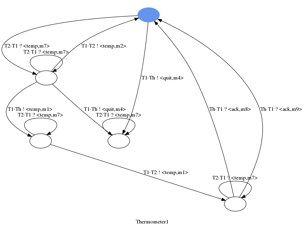
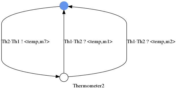
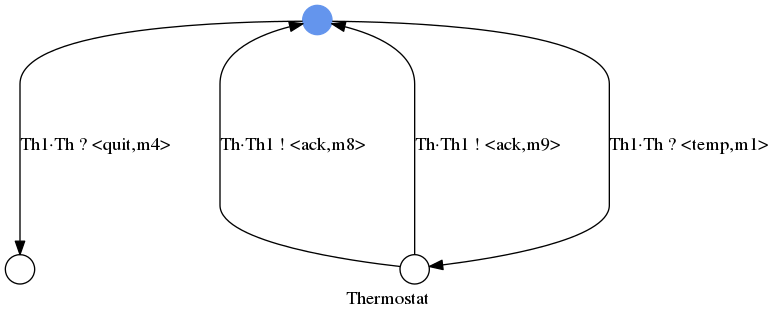
Figure 7: CFSMs of the amended specification ACC

Our next step is to verify communication, in particular, to detect the presence of dangling or missing messages left and of deadlocks. To do that, we use ChorGram to check if the system enjoys the generalised multiparty compatibility (GMC) mentioned in Section 2.1 and described later. To check GMC, ChorGram analyses the CFSMs of the system against their synchronous executions, that is the finite labelled transition system (STS for short) obtained by executing the system with two additional constraints: (i) a message could be sent only if the receiving partner is ready to consume the message and (ii) all buffers are empty.

A system of CFSMs enjoys the GMC property when it is representable and has the branching property [15]. The representability condition essentially requires that for each participant, the projection of the STS onto that participant yields a CFSM bisimilar to the original machine. The branching property condition requires that whenever a branching occurs in the STS then either ($i$) the branching commutes, i.e. it corresponds to two independent (concurrent) interactions, or ($ii$) it corresponds to a choice that meets the following constraints:

1. there is a single participant, dubbed the selector, that “decides” which branch to take, and

2. any participant not acting as a selector either has the same behaviour in each branch or it behaves differently in any branch of the choice.

Item (1) guarantees that every choice is located at exactly one participant (this is crucial since we are assuming asynchronous communications). Item (2) ensures that all the other participants are either unaware of the choice or, if they are involved, they can distinguish which branch is taken by the selector. We recall that the GMC property ensures communication soundness, i.e. that systems are deadlock-free and they are not message oblivious.

Giving the machines for ACC (cf. Section 4) as input to ChorGram we obtain the following STS:

where, for legibility, we adopt the abbreviations used in Section 3 and omit the identities of irrelevant states. The configurations of the STS are made of the states of the (minimised) CFSMs of ACC separated by a dot; for instance, the left-most state in the STS above represents a configuration in which the local state of (the CFSM of) Th₁ is (the equivalence class containing the) state $\mathsf{q30,q31}$, Th₂ is in state $\mathsf{q6,q7}$, and Th is in state $\mathsf{q14}$. This configuration, call it $c$, is reached when, from the initial configuration, Th₁ decides to send Th the quit message, as described by the left-most transition. Note that ChorGram decorates this transition with the STS with the “No choice awareness” message to highlight that a potential violation of the branching property occurs at the source state of the transition (which is the initial state of the STS). Indeed, configuration $c$ has a transition to a deadlock configuration, also highlighted by ChorGram, hence detecting a communication problem of ACC.

To investigate and fix the problem we analyse the STS and the global graph computed by ChorGram on the machines depicted in Figure 7.

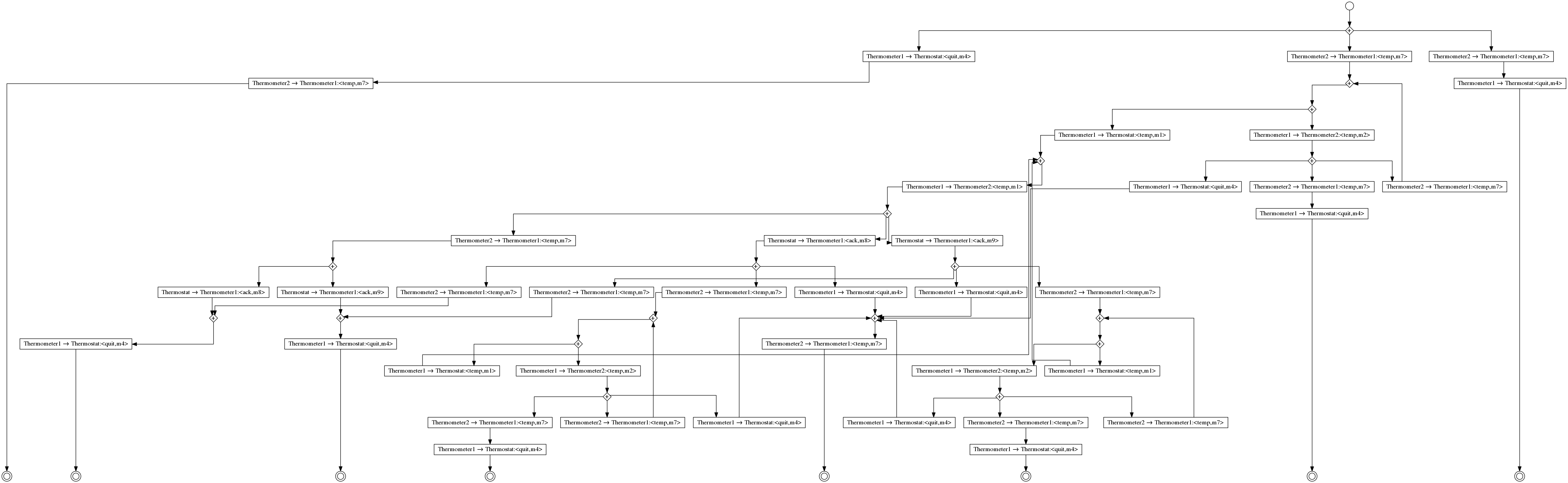
Figure 8: The global graph of the communication-unsound ACC

Albeit not fully readable, we show the global graph in Figure 8 to give an idea of the complex interactions that our simple scenario generates. By inspecting this global graph we note that there are paths to sink nodes. This is not expected of ACC since each component is supposed to perpetually execute its loop. Therefore, those paths should be related to the reachable deadlock configuration of the STS.

We start by analysing the left-most path ending in the sink node ​​ of Figure 8 starting from the initial node ​ in the graph. This path describes a very short interaction only consisting of two exchanged messages in which Th₁ first sends message quit to Th and then receives the value of the temperature computed by Th₂. By inspecting the code in Figure 3, the attentive designer would observe that the first interaction corresponds to the send performed by the first process of Th₁ at line 33. After sending the quit message, the first process of Th₁ ends and makes the thermostat Th to terminate as well (lines 17-19 of Figure 2). Hence, the second interaction on the path under consideration can only happen between Th₂ and the second process of Th₁. After sending its message Th₂ waits for a reply from Th₁ (line 51 of Figure 3); however, the second process of Th₁ sends no messages, it only waits for incoming ones. Thus, a deadlock occurs because Th₁ and Th₂ are waiting each to receive from the other.

By inspecting the rest of the global graph, we discover that the other deadlocks are caused by the same sequence of interactions: a deadlock occurs as soon as Th₁ sends the message quit to the thermostat. The problem arises because the second process of Th₁ never acknowledges the message received by the other thermometer. This is a violation of condition (2) of GMC (see page 2). As highlighted in the STS, there is no choice awareness since the decision of quitting is not properly propagated to all participants. To fix this problem we change the code of the second process Th₁: we insert a send construct as shown in Figure 6, line 5, so that the process replies to each message of Th₂.

Then, we re-apply ChorGram on the new version of our system and this time ChorGram shows it is GMC, so establishing its communication soundness. Indeed, the extra communication from Th₁ to Th₂ now ensures that the thermometer Th₂ behaves uniformly when communicating with Th₁. The combination of the two analyses is therefore guaranteeing that our last version of ACC does not mis-compute or mis-communicate data.

6 Conclusions

We proposed the combination of a control flow analysis and the analysis of communication soundness based on a choreographic framework as complementary approaches for the formal verification of IoT systems. Both analyses and the interface between them are tool supported, although the constraint solver for the first is still under development. Our approach has been illustrated within a scenario that, albeit conceptually simple, highlights non-trivial issues that designers of IoT applications should tackle. Indeed, tool support is crucial in this context since the high level of non-determinism that IoT systems exhibit makes it is hard for the designer to model robust applications.

For specifying IoT systems we appealed to IoT-LySa, a recently proposed formalism based on a process calculus and tailored to model monitoring system made of smart devices that communicate, make computations on sensed data, and command actuators. It is endowed with a control flow analysis that allows the designer to identify points of the system where computations are not as expected, both on the way data are aggregated and on the way communications occur among the smart objects.

Once the designer has attained a system correct from the point of view of local computations, communication properties are verified by checking that the components of the IoT specification form a valid choreography using the ChorGram tool. To link together the two analyses we implemented a compiler that translates a system specification into a set of CFSMs. The compiled system soundly reflects the communication behaviour of the original specification, ensuring that each property proved by ChorGram, also holds for the IoT-LySa specification. During our experiments, ChorGram has sometimes singled out unexpected communications. In particular, the complexity of the communication pattern of our scenario was not fully understood before putting it under the lens of ChorGram, even though our working examples were conceptually simple.

This paper is a first attempt to study the entanglement between local computations and distributed interactions. In our opinion, this issue is of uttermost relevance in IoT systems, as already discussed in Section 1. We are currently exploring how the combination of IoT-LySa and its analysis with ChorGram could be used for verifying more sophisticated properties of IoT systems. In particular, we believe that the global model of an IoT system returned by ChorGram could help us in refining the results of the control flow analysis. Indeed, the global model yields a more precise description of the flow of data induced by actual communications than the current analysis of IoT-LySa can only approximate, unless one makes it more complex and computationally expensive. Improving the precision of the CFA facilitates detecting erroneous communications and misuse of data caused by them. We further plan to investigate the definition of a modal logic for expressing and model checking a variety of properties about communication and dependency of data on the global graph obtained by using our approach.

Appendix A IoT-LySa Syntax

The syntax of systems is as follows.

$$\begin{array}[]{ll@{\hspace{2ex}}l}{\mathcal{N}}\ni N::=&{\it systems\ of\ nodes}\hfil\hskip 6.02777pt&\\ &\mathbf{0}\hfil\hskip 6.02777pt&\hbox{empty system}\\ &\ell:[B]\hfil\hskip 6.02777pt&\hbox{single node}\;(\ell\in{\mathcal{L}})\\ &N_{1}\ |\ N_{2}\hfil\hskip 6.02777pt&\hbox{parallel composition of nodes}\end{array}\quad\begin{array}[]{ll@{\hspace{2ex}}l}{\mathcal{B}}\ni B::=&\text{\it node components}\hfil\hskip 6.02777pt&\\ &\Sigma_{\ell}\hfil\hskip 6.02777pt&\hbox{store of node }\ell\\ &P\hfil\hskip 6.02777pt&\hbox{process}\\ &S\hfil\hskip 6.02777pt&\hbox{sensor, with a unique id $i\in\mathcal{I}_{\ell}$}\\ &A\hfil\hskip 6.02777pt&\hbox{actuator, with a unique id $j\in\mathcal{J}_{\ell}$}\\ &B\ \|\ B\hfil\hskip 6.02777pt&\hbox{parallel composition of components}\end{array}$$

$$\begin{array}[]{lll}{\mathcal{P}}\ni P::=&{\it control\ processes}&\\ &\mathbf{0}&\hbox{inactive process}\\ &{\langle}\!\langle{E_{1},\cdots,E_{r}}{\rangle}\!\rangle\triangleright{{L}}.\,P&\hbox{asynchronous multi-output L$\subseteq{\mathcal{L}}$}\\ &{\langle}\!\langle{c_{1},\cdots,c_{j},E_{j+1}\cdots E_{r}}{\rangle}\!\rangle\triangleright{{L}}.\,P&\hbox{asynchronous multi-output (with tags)}\\ &{(}{E_{1},\cdots,E_{j}}{;}\ {x_{j+1},\cdots,x_{r}}{)}.\,{P}&\hbox{input}\\ &{(}{c_{1},\cdots,c_{j}}{;}\ {x_{j+1},\cdots,x_{r}}{)}.\,{P}&\hbox{input (with tags) }\\ &{(}{c_{1},\cdots,c_{j}}{;}\ {x_{j+1},\cdots,x_{r}}{)}.\,{P}+\\ &{(}{c^{\prime}_{1},\cdots,c^{\prime}_{j}}{;}\ {x^{\prime}_{j+1},\cdots,x^{\prime}_{r}}{)}.\,{Q}&\hbox{switch or external choice }\\ &E?P:Q&\hbox{conditional statement}\\ &h&\hbox{iteration variable}\\ &\mu h.\ P&\hbox{iteration}\par\\[0.60275pt] &x:=E.\,P&\hbox{assignment to $x\in{\mathcal{X}}_{\ell}$}\\ &{\langle}{j,\gamma}{\rangle}.\,{{P}}&\hbox{output of action $\gamma$ to actuator $j$}\end{array}\quad\begin{array}[]{ll@{\hspace{2ex}}l}\\ \\ {\mathcal{E}}\ni E::=&{\it terms}\hfil\hskip 6.02777pt&\\ &v\hfil\hskip 6.02777pt&\hbox{value }(v\in{\mathcal{V}})\\ &i\hfil\hskip 6.02777pt&\hbox{sensor location }(i\in{\mathcal{I}_{\ell}})\\ &x\hfil\hskip 6.02777pt&\hbox{variable }(x\in{\mathcal{X}}_{\ell})\\ &f(E_{1},\cdots,E_{r})\hfil\hskip 6.02777pt&\hbox{function on data }(f\in{\mathcal{F}})\\ \end{array}$$

$$\begin{array}[]{ll@{\hspace{2ex}}l ll@{\hspace{2ex}}l}S&::={\it sensors}\hfil\hskip 6.02777pt&&A&::={\it actuators}\hfil\hskip 6.02777pt&\\ &\mathbf{0}\hfil\hskip 6.02777pt&\hbox{inactive sensor}&&\mathbf{0}\hfil\hskip 6.02777pt&\hbox{inactive actuator}\\ &\tau.S\hfil\hskip 6.02777pt&\hbox{internal action}&&\tau.A\hfil\hskip 6.02777pt&\hbox{internal action}\\ &probe(i).\,{S}\hfil\hskip 6.02777pt&\hbox{sense a value by}&&(\!|j,\Gamma|\!).\,A\hfil\hskip 6.02777pt&\hbox{command for actuator $j$}\\ &\hfil\hskip 6.02777pt&\hbox{the $i^{th}$ sensor}&&\gamma.A\hfil\hskip 6.02777pt&\hbox{triggered action ($\gamma\in\Gamma$)}\par\\ &h\hfil\hskip 6.02777pt&\hbox{iteration variable}&&h\hfil\hskip 6.02777pt&\hbox{iteration variable}\\ &\mu h\,.\,S\hfil\hskip 6.02777pt&\hbox{iteration}&&\mu h\,.\,A\hfil\hskip 6.02777pt&\hbox{iteration}\end{array}$$

We briefly comment on the output and input constructs. The prefix ${\langle}\!\langle{E_{1},\cdots,E_{r}}{\rangle}\!\rangle\triangleright{{L}}$ implements a simple multicast communication: the tuple $E_{1},\dots,E_{r}$ is asynchronously sent to the nodes in $L$. The input prefix $(E_{1},\!\cdots\!,E_{j};x_{j+1},\!\cdots\!,x_{r})$ receives a $r$-tuple, provided that its first $j$ terms match the input ones, and then binds the remaining store variables (separated by a “;”) to the corresponding values. Otherwise, the $r$-tuple is not accepted. The present variant of IoT-LySa has external choices not originally included in [10, 9] that is rendered by two branches guarded by two different input actions. Note that input and output actions may contain tags $c\in\mathcal{C}$.

For instance the process included in the thermostat node Th in Figure 2, is specified as follows.

$$P_{\mathsf{Th}}=\mu\mathsf{h}. (\mathsf{temp};\mathsf{x}).(\mathsf{tthreshold}<\mathsf{x})\ ?\$$

$$\qquad{\langle}{\mathsf{ACon\_off,on}}{\rangle}.\,{{}}{\langle}\!\langle{\mathsf{ack},\mathsf{on}}{\rangle}\!\rangle\triangleright{{\{\mathsf{Th_{1}}\}}}\ .\ \mathsf{h}:$$

$$\qquad{\langle}{\mathsf{ACon\_off,off}}{\rangle}.\,{{}}{\langle}\!\langle{\mathsf{ack},\mathsf{off}}{\rangle}\!\rangle\triangleright{{\{\mathsf{Th_{1}}\}}}\ .\ \mathsf{h}$$

$$\ +(\mathsf{quit};\mathsf{i}).\mathbf{0}$$

Appendix B Mapping IoT-LySa to CFSMs

Here, we detail the procedures described in Section 4 for compiling an IoT-LySa specification into a set of CFSMs. First, we define the simplification procedure that substitutes fresh variables for expressions in input/output prefixes. This transformation is inductively defined on the syntax of the system of nodes:

Definition B.1.

Let $N$ be an IoT-LySa system of nodes, the procedure $\mathit{simpl}\colon\mathcal{N}\to\mathcal{N}$ is inductively defined below, where we use two auxiliary functions $\mathit{simpl_{B}}\colon\mathcal{B}\to\mathcal{B}$ and $\mathit{simpl_{P}}\colon\mathcal{P}\to\mathcal{P}$.

$$\begin{array}[]{ll}\begin{array}[]{ll}\mathit{simpl}(\mathbf{0})&=\,\mathbf{0}\\ \mathit{simpl}(\ell:[B])&=\,\ell:[\mathit{simpl_{B}}(B)]\\ \mathit{simpl}(N_{1}\mid N_{2})&=\,\mathit{simpl}(N_{1})\mid\mathit{simpl}(N_{2})\end{array}&\begin{array}[]{ll}\mathit{simpl_{B}}(P)&=\,\mathit{simpl_{P}}(P)\\ \mathit{simpl_{B}}(B_{1}\parallel B_{2})&=\,\mathit{simpl_{B}}(B_{1})\parallel\mathit{simpl_{B}}(B_{2})\\ \mathit{simpl_{B}}(X)&=\,X\qquad\text{for }X\in\{\Sigma_{\ell},\,S,\,A\}\end{array}\end{array}$$

$$\begin{array}[]{ll}\mathit{simpl_{P}}(X)&=\,X\\ &\qquad\text{for }X\in\{\mathbf{0},\,h\}\\ \mathit{simpl_{P}}(Y.P)&=\,Y.\mathit{simpl_{P}}(P)\\ &\qquad\text{for }Y\in\{\mu h,\,x:=E,\,\langle j,\gamma\rangle\}\\ \mathit{simpl_{P}}(E?P_{1}:P_{2})&=\,E\,?\,\mathit{simpl_{P}}(P_{1}):\mathit{simpl_{P}}(P_{2})\\ \mathit{simpl_{P}}({\langle}\!\langle{E_{1},\cdots,E_{r}}{\rangle}\!\rangle\triangleright{{L}}.\,P)&=\,{\langle}\!\langle{m_{1},\cdots,m_{r}}{\rangle}\!\rangle\triangleright{{L}}.\,\mathit{simpl_{P}}(P)\\ &\qquad m_{1},\dots,m_{r}\text{ fresh variables}\\ \mathit{simpl_{P}}({\langle}\!\langle{c_{1},\cdots,c_{j},E_{j+1},\cdots,E_{r}}{\rangle}\!\rangle\triangleright{{L}}.\,P)&=\,{\langle}\!\langle{c_{1},\cdots,c_{j},m_{j+1},\cdots,m_{r}}{\rangle}\!\rangle\triangleright{{L}}.\,\mathit{simpl_{P}}(P)\\ &\qquad m_{j+1},\dots,m_{r}\text{ fresh variables}\\ \mathit{simpl_{P}}({(}{E_{1},\cdots,E_{j}}{;}\ {x_{j+1},\cdots,x_{r}}{)}.\,{P})&=\,{(}{m_{1},\cdots,m_{j}}{;}\ {m_{j+1},\cdots,m_{r}}{)}.\,{\mathit{simpl_{P}}(P)}\\ &\qquad m_{1},\dots,m_{r}\text{ fresh variables}\\ \mathit{simpl_{P}}(\sum^{2}_{i=1}{(}{c^{i}_{1},\cdots,c^{i}_{j}}{;}\ {x^{i}_{j+1},\cdots,x^{i}_{r}}{)}.\,{P_{i}})&=\,\sum^{2}_{i=1}{(}{c^{i}_{1},\cdots,c^{i}_{j}}{;}\ {m^{i}_{j+1},\cdots,m^{i}_{r}}{)}.\,{\mathit{simpl_{P}(P_{i})}}\\ &\qquad m^{i}_{j+1},\dots,m^{i}_{r}\,\text{ fresh variables}\end{array}$$

Applying the above procedure to the IoT-LySa process $P_{Th}$ above results in:

$$\mathit{simpl_{P}}(P_{\mathsf{Th}})=\mu\mathsf{h}. (\mathsf{temp};m_{x}).(\mathsf{tthreshold}<\mathsf{x})\ ?\$$

$$\qquad{\langle}{\mathsf{ACon\_off,on}}{\rangle}.\,{{}}{\langle}\!\langle{\mathsf{ack},m_{\mathsf{on}}}{\rangle}\!\rangle\triangleright{{\{\mathsf{Th_{1}}\}}}\ .\ \mathsf{h}:$$

$$\qquad{\langle}{\mathsf{ACon\_off,off}}{\rangle}.\,{{}}{\langle}\!\langle{\mathsf{ack},m_{\mathsf{off}}}{\rangle}\!\rangle\triangleright{{\{\mathsf{Th_{1}}\}}}\ .\ \mathsf{h}$$

$$\ +(\mathsf{quit};m_{\mathsf{i}}).\mathbf{0}$$

For brevity, we omitted above the straightforward computation of the environment. Indeed, it sufficies modifying each procedure to return a pair whose second element is the environment; to deal with recursive calls, e.g. in the case $E?P_{1}:P_{2}$, we combine the returned mappings to form the overall one.

Below, we formalise the compilation of a process inside an IoT-LySa node into an automaton. This procedure operates on processes whose input/output prefixes only contain tags and fresh variables (cf. Definition B.1). We assume the standard definition of a finite state machine as a tuple $(S,s,F,\Sigma,\delta)$. We define the function $\mathcal{A}\llbracket\_\rrbracket\_$ that takes a process, a component $\kappa$ of the CFA (modified in step 2 of Section 4, (e.g. $(\mathsf{Th},\mbox{\guillemotleft}{\mathsf{ack},m_{\mathsf{on}}}\mbox{\guillemotright}\in\kappa(\mathsf{Th_{1}})$ in $P_{\mathsf{Th}}$) and returns a CFSM. The obtained machine implements the same communication behaviour of the process. For the sake of readability, in the following definition we do not explicitly show the alphabet set of the automata (simply the union of the alphabets of the automata returned by recursive calls and of the symbols (different from $\epsilon$) occurring in the transition relation $\delta$). Furthermore, when needed we assume to generate new states, e.g. $s_{i}$ and $s_{f}$.

Definition B.2.

Let $P$ be an IoT-LySa process of the node $\ell$, and $\kappa$ be the CFA component (simplified in step 2 of Section 4). Then, the translation $\mathcal{A}\llbracket\_\rrbracket\_\colon\mathcal{P}\to\mathcal{K}\to CFSM$ is inductively defined as follows:

$$\begin{array}[]{ll}\mathcal{A}\llbracket\mathbf{0}\rrbracket\kappa&=\,(\{s_{i}\},s_{i},\emptyset,\emptyset)\\ \mathcal{A}\llbracket h\rrbracket\kappa&=\,(\{s_{i},\,s_{f}\},s_{i},\{s_{f}\},\{(s_{i},\epsilon,s_{f})\})\\ \mathcal{A}\llbracket Y.P\rrbracket\kappa&=\,(\{s_{i}\}\cup S^{P},s_{i},F^{P},\delta^{P}\cup\{(s_{i},\tau,s^{P}_{i})\})\\ &\,\,\text{where }Y\in\{x:=E,\langle j,\gamma\rangle\}\,\,\text{ and }\mathcal{A}\llbracket P\rrbracket\kappa=(S^{P},s^{P}_{i},F^{P},\delta^{P})\\ \mathcal{A}\llbracket E?P:Q\rrbracket\kappa&=\,(\{s_{i},s_{f}\}\cup S^{P}\cup S^{Q},s_{i},\{s_{f}\},\delta^{P}\cup\delta^{Q}\cup\\ &\,\cup\{(s_{i},\epsilon,s^{P}_{i}),(s_{i},\epsilon,s^{P}_{i})\}\cup\{(s,\epsilon,s_{f})\mid s\in F^{P}\cup F^{Q}\})\\ &\,\,\text{where }\mathcal{A}\llbracket P\rrbracket\kappa=(S^{P},s^{P}_{i},F^{P},\delta^{P})\,\,\text{ and }\mathcal{A}\llbracket Q\rrbracket\kappa=(S^{Q},s^{Q}_{i},F^{Q},\delta^{Q})\\ \mathcal{A}\llbracket{\langle}\!\langle{m_{1},\cdots,m_{r}}{\rangle}\!\rangle\triangleright{{L}}.\,P\rrbracket\kappa&=\,(\{s_{i},\,s_{1},\,\dots,\,s_{n}\}\cup S^{P},s_{i},F^{P},\delta^{P}\cup\bigcup^{n-1}_{i=0}(s_{i},e_{i+1},s_{i+1})\cup\{(s_{n},\,\epsilon,s^{P}_{i})\})\\ &\,\,\text{ where }\mathcal{A}\llbracket P\rrbracket\kappa=(S^{P},s^{P}_{i},F^{P},\delta^{P}),\\ &\,\,s_{1},\dots,s_{n}\text{ new, }L=\{\ell_{1},\dots,\ell_{n}\}\\ &\,\,\text{ and }e_{i+1}=\ell\cdot\ell_{i+1}!\mbox{\guillemotleft}{m_{1},\dots,m_{r}}\mbox{\guillemotright}\\ \mathcal{A}\llbracket{\langle}\!\langle{m_{1},\cdots,m_{r}}{\rangle}\!\rangle\triangleright{{L}}.\,P\rrbracket\kappa&=\,(\{s_{i},\,s_{1},\,\dots,\,s_{n}\}\cup S^{P},s_{i},F^{P},\delta^{P}\cup\bigcup^{n-1}_{i=0}(s_{i},e_{i+1},s_{i+1})\cup\{(s_{n},\,\epsilon,s^{P}_{i})\})\\ &\,\,\text{ where }\mathcal{A}\llbracket P\rrbracket\kappa=(S^{P},s^{P}_{i},F^{P},\delta^{P}),\\ &\,\,s_{1},\dots,s_{n}\text{ new, }L=\{\ell_{1},\dots,\ell_{n}\}\\ &\,\,\text{ and }e_{i+1}=\ell\cdot\ell_{i+1}!\mbox{\guillemotleft}{m_{1},\dots,m_{r}}\mbox{\guillemotright}\\ \mathcal{A}\llbracket{\langle}\!\langle{c_{1},\cdots,c_{j},m_{j+1},\cdots,m_{r}}{\rangle}\!\rangle\triangleright{{L}}.\,P\rrbracket\kappa&=\,(\{s_{i},\,s_{1},\,\dots,\,s_{n}\}\cup S^{P},s_{i},F^{P},\delta^{P}\cup\bigcup^{n-1}_{i=0}(s_{i},e_{i+1},s_{i+1})\cup\{(s_{n},\,\epsilon,s^{P}_{i})\})\\ &\,\,\text{ where }\mathcal{A}\llbracket P\rrbracket\kappa=(S^{P},s^{P}_{i},F^{P},\delta^{P}),\\ &\,\,s_{1},\dots,s_{n}\text{ new, }L=\{\ell_{1},\dots,\ell_{n}\}\\ &\,\,\text{ and }e_{i+1}=\ell\cdot\ell_{i+1}!\mbox{\guillemotleft}{c_{1},\dots,c_{j},m_{j+1},\dots,m_{r}}\mbox{\guillemotright}\\ \mathcal{A}\llbracket{(}{m_{1},\cdots,m_{j}}{;}\ {m_{j+1},\cdots,m_{r}}{)}.\,{P}\rrbracket\kappa&=\,(\{s_{i}\}\cup S^{P},s_{i},F^{P},\delta^{P}\cup\bigcup_{(\ell^{\prime},t)\in\kappa(\ell)}(s_{i},\ell\cdot\ell^{\prime}?t,s^{P}_{i}))\\ &\,\,\text{ where }\mathcal{A}\llbracket P\rrbracket\kappa=(S^{P},s^{P}_{i},F^{P},\delta^{P})\\ \mathcal{A}\llbracket\sum^{2}_{i=1}{(}{c^{i}_{1},\cdots,c^{i}_{j}}{;}\ {m^{i}_{j+1},\cdots,m^{i}_{r}}{)}.\,{P_{i}}\rrbracket\kappa&=\,(\{s_{i}\}\cup\bigcup^{2}_{i=1}S^{P_{i}},\bigcup^{2}_{i=1}F^{P_{i}},\bigcup^{2}_{i=1}\delta^{P_{i}}\cup\bigcup_{(\ell^{\prime},t)\in\kappa(\ell)}(s_{i},\ell\cdot\ell^{\prime}?t,s^{P_{i}}_{i})\\ &\,\,\text{ where }\mathcal{A}\llbracket P_{i}\rrbracket\kappa=(S^{P_{i}},s^{P_{i}}_{i},F^{P_{i}},\delta^{P_{i}})\\ \end{array}$$

Applying this translation to $P_{Th}$ results in the right-bottom automaton in Figure 7.

References

- [1]
- [2] Business Process Model and Notation. http://www.bpmn.org.
- [3] Compiler from IoT-LySa to CFSMs. https://bitbucket.org/lillo/iotlysa.
- [4] Alfred V. Aho, Ravi Sethi & Jeffrey D. Ullman (1986): Compilers: Principles, Techniques, and Tools. Addison-Wesley.
- [5] Amber Ankerholz (2017): Bruce Schneier on New Security Threats from the Internet of Things. https://www.linux.com/news/event/open-source-leadership-summit/2017/3/bruce-schneier-new-security-threats-internet-things. Linux.com interviews Bruce Schneier.
- [6] Massimo Bartoletti, Alceste Scalas, Emilio Tuosto & Roberto Zunino (2016): Honesty by Typing. Logical Methods in Computer Science 12(4), 10.2168/LMCS-12(4:7)2016.
- [7] Laura Bocchi, Julien Lange & Nobuko Yoshida (2015): Meeting Deadlines Together. In: CONCUR 2015, pp. 283–296, 10.4230/LIPIcs.CONCUR.2015.283.
- [8] Chiara Bodei, Mikael Buchholtz, Pierpaolo Degano, Flemming Nielson & Hanne Riis Nielson (2005): Static validation of security protocols. Journal of Computer Security 13(3), pp. 347–390, 10.3233/JCS-2005-13302.
- [9] Chiara Bodei, Pierpaolo Degano, Gian-Luigi Ferrari & Letterio Galletta (2016): A step towards checking security in IoT. In: Procs. of ICE 2016, EPTCS 223, pp. 128–142, 10.4204/EPTCS.223.9.
- [10] Chiara Bodei, Pierpaolo Degano, Gian-Luigi Ferrari & Letterio Galletta (2016): Where do your IoT ingredients come from? In: Procs. of Coordination 2016, LNCS 9686, Springer, pp. 35–50, 10.1007/978-3-319-39519-7.
- [11] Chiara Bodei, Pierpaolo Degano, Gian-Luigi Ferrari & Letterio Galletta (2017): Tracing where IoT data are collected and aggregated. Logical Methods in Computer Science 13(3:5), pp. 1–38, 10.23638/LMCS-13(3:5)2017.
- [12] Daniel Brand & Pitro Zafiropulo (1983): On Communicating Finite-State Machines. Journal of the ACM 30(2), pp. 323–342, 10.1145/322374.322380.
- [13] Pierre-Malo Deniélou & Nobuko Yoshida (2012): Multiparty Session Types Meet Communicating Automata. In: ESOP 2012, pp. 194–213, 10.1007/978-3-642-28869-2_10.
- [14] Julien Lange & Emilio Tuosto (2015): ChorGram: tool support for choreographic development. Available at https://bitbucket.org/emlio_tuosto/chorgram/wiki/Home.
- [15] Julien Lange, Emilio Tuosto & Nobuko Yoshida (2015): From Communicating Machines to Graphical Choreographies. In: POPL15, pp. 221–232, 10.1145/2676726.2676964.
- [16] Julien Lange, Emilio Tuosto & Nobuko Yoshida (2017): A tool for choreography-based analysis of message-passing software. To appear. Available at http://www.cs.le.ac.uk/~et52/chorgram_betty_ch.pdf.
- [17] Robin Milner (1993): Elements of Interaction Turing Award Lecture. CACM 36(1), 10.1145/151233.151240.