Safe Exploration for Identifying Linear Systems via Robust Optimization

Abstract

Safely exploring an unknown dynamical system is critical to the deployment of reinforcement learning (RL) in physical systems where failures may have catastrophic consequences. In scenarios where one knows little about the dynamics, diverse transition data covering relevant regions of state-action space is needed to apply either model-based or model-free RL. Motivated by the cooling of Google’s data centers, we study how one can safely identify the parameters of a system model with a desired accuracy and confidence level. In particular, we focus on learning an unknown linear system with Gaussian noise assuming only that, initially, a nominal safe action is known. Define safety as satisfying specific linear constraints on the state space (e.g., requirements on process variable) that must hold over the span of an entire trajectory, and given a Probably Approximately Correct (PAC) style bound on the estimation error of model parameters, we show how to compute safe regions of action space by gradually growing a ball around the nominal safe action. One can apply any exploration strategy where actions are chosen from such safe regions. Experiments on a stylized model of data center cooling dynamics show how computing proper safe regions can increase the sample efficiency of safe exploration.

1 Introduction

Applying reinforcement learning (RL) to control physical systems in complex, failure-prone environments is non-trivial. The advantages of RL is significant: deploying an agent that is able to learn and optimally control a sophisticated physical system reduces the amount of manual tuning, hard-coding and guess work that goes in to designing good controllers in many applications.

However, a key problem in an unknown system is that the RL agent must explore to learn the relevant aspects of the dynamics for optimal control. Furthermore, in a failure-sensitive environment, the agent must explore without triggering unsafe events. This is known as the safe exploration problem and has recently gained prominence in both the research community and the broader public consciousness [10, 1, 22]. This interest has also been driven by some recent successes of RL over traditional control regimes for physical systems such as those for controlling pumps, chillers and cooling towers for data centers [8].

In this paper, we focus a critical aspect of model-based RL control, namely, system identification subject to safety constraints. Specifically, working with linear Gaussian dynamics models—motivated by a data center cooling system control at Google—we define safety w.r.t. a domain-specific set of linear constraints over state variables that must be satisfied at all times. This is the common notion of safety in industrial applications where certain process variables (system state variables being monitored or controlled) should meet certain target set points, and must not diverge more than a fixed amount from those points. Once a system dynamics model is learned to a sufficient degree, it can be used in a model-based RL or other control algorithm.

Unlike recent work that takes a Bayesian approach to modelling system uncertainty, we adopt a strict uncertainty perspective, and reason with a set of models within which the true system model must lie with high probability. The set itself is defined using PAC-style bounds derived from an exploration data set over state-action space. With this perspective, we compute safe regions of action space where, starting with an initial state, one can take any sequence of actions within the safe region and guarantee satisfaction of the (state) safety constraints on the states at every step of the trajectory.

Our approach assumes the existence of a nominal safe action, namely, an action that is safe in the sense that it, if continuously applied, will eventually drive the system to a safe state no matter what the initial state, and will maintain safety in steady state. A safe region is then computed by gradually growing a ball around the nominal action, or some other action known to be safe. Our experiments use a modified version of the linear-Gaussian dynamics of a data center’s cooling system. We show how our algorithms can be used to efficiently and safely explore while also computing high probability bounds on the estimated model quality.

2 Related Work

Given our definition of safety, perhaps the most relevant work is that of Akametalu et al. [14], who require that, during exploration, the states at every time step must reside within a pre-defined region of safety. They focus on computing a subset of the safe states $D$ with the property that, when starting from any initial state in $D$, one can execute any exploration policy as long as certain safe actions are taken when the state starts drifting out of $D$. However, computation of $D$ scales exponentially in the state dimension. The transition dynamics are assumed to be partially known but a deterministic disturbance function is unknown and modeled as a Gaussian process (GP). While their safety definition bears a close resemblance to ours, we determine safe regions of action space as a function of the initial state rather than computing safe initial states from which to explore. Furthermore, we do not assume any prior knowledge of the dynamics model and instead treat model uncertainty with PAC-like bounds on the quality of least-squares parameter estimates. Safe exploration with a finite state space, known deterministic transition and an uncertain safety function modeled with a GP is studied by Turchetta et al. [26], who develop an exploration algorithm with provable safety guarantees. Several other lines of work also use GPs for safe exploration [27, 25, 4]. Our approach is not Bayesian, and does not explicitly encounter computational complexity issues often associated with Bayesian inference.

Our approach, using robust optimization of a worst-case safety violation, is somewhat related to robust MDPs (RMDPs) [21, 13]. In RMDPs one assumes the true model lies in a smaller model set $\Theta$ defined by an error upper bound on the transition probabilities, then the goal is to optimize a policy that performs best with respect to an adversarial choice of the true transition model in $\Theta$. We also work with a model set $\Theta$ where the true model lies with high probability but instead of optimizing a policy (where one can also encode safety constraints) we are interested in finding safe action regions. Recent work [11] considers the RMDP setting where the safety goal is to find a policy that performs better than some baseline policy, with most of the analysis in the finite-state setting, and methods that do not easily scale to continuous, multi-dimensional state spaces. Similar work [9, 15] also tries to improve on a baseline policy. We do not assume a safe baseline policy exists, but instead assume a known safe action (see above).

System identification is a well-studied topic in control theory [23, 18, 3]. Typically it consists of three phases: (1) data gathering; (2) model class selection; and (3) parameter estimation [18]. In this work, we primarily deal with in safe exploration for data gathering and parameter estimation in the context, quantifying the approximation quality of parameter estimates and using this as a stopping criterion for exploration. With regard to model class selection, various model types are studied in the literature, including ARX (autoregressive with exogenous inputs), ARMA (autoregressive moving average) and ARMAX (autoregressive moving average with exogeneous inputs) [5]. Our paper focuses on learning linear ARX models as opposed to non-linear models, such as neural networks [6]. For exploration, the celebrated result on persistently exciting inputs [2] asserts that control input signals that are rich enough—having a certain number of distinct frequencies—provide sufficiently diverse training data to learn the true model. We leverage this insight in our work.

In the context of robust parameter estimation, there is a line of work on bounded noise models in system identification [29, 24, 28]. This paradigm does not assume any statistical form of the noise inherent in state observations, but instead assumes only that the noise is bounded by an unknown constant. Researchers have studied the existence and characteristics of estimators for various optimality concepts [19]. In our setting, we assume a statistical distribution for the noise model, but we compute robust, safe actions with respect to the uncertainty in the model parameters estimated from trajectory data.

3 Preliminaries

We first describe some basic concepts and notation related to sequential decision making. Since our paper’s main results center on linear transition models with Gaussian noise, we address this model class in some detail and outline some corresponding PAC-style bounds for estimating the parameters of these models. These bounds depend on properties of the training data—generally, a time series of system behaviour—and thus do not require that training examples be independently generated.

3.1 Background and Notation

Let $\mathcal{X}\subseteq\mathbb{R}^{d}$ be the state space and $\mathcal{U}\subseteq\mathbb{R}^{d^{\prime}}$ the action space. We generally view each dimension of the state as representing some process variable to be monitored or controlled, and each action dimension as some control variable to be set. For example, the state might be a vector of sensor readings while the action might be a vector of hardware parameter configurations. Let $\mathbf{x}_{t}\in\mathcal{X}$ denote the system state at time $t$ and $x_{t\ell}$ the value of its $\ell$-th variable, for $t\in\{0,1,2,\ldots\}$. Likewise, let $\mathbf{u}_{t}\in\mathcal{U}$ be the action taken at time $t$ in state $\mathbf{x}_{t}$. There is an underlying, unknown transition model $P^{*}(\mathbf{x}_{t+1}~{}|~{}\mathbf{x}_{t},\mathbf{u}_{t})$, i.e., the distribution from which the state at the next time step $\mathbf{x}_{t+1}$ is generated. The transition model is stationary and Markovian (i.e., depends only on the current state $\mathbf{x}_{t}$ and action $\mathbf{u}_{t}$).

We consider time-based episodes or trajectories of state-action sequences: $(\mathbf{x}_{0},\mathbf{u}_{0}),\ldots,(\mathbf{x}_{T-1},\mathbf{u}_{T-1}),(\mathbf{x}_{T})$. A length $T$ episodes is typically generated by providing initial state $\mathbf{x}_{0}$ to our agent, which executes an exploration policy that selects/executes action $\mathbf{u}_{t}$ in response to observing state $\mathbf{x}_{t}$ (and past history), which induces $\mathbf{x}_{t+1}$ according the true system dynamics, for $T-1$ stages. The initial state $\mathbf{x}_{0}$ might be exogeneously realized and may differ across episodes. Our goal is to ensure safety during an episode.

We use the following notation throughout. Let $\mathbf{v}_{i:j}=\mathbf{v}_{i},\ldots,\mathbf{v}_{j}$ denote a sequence of $j-i+1$ vectors starting at index $i$. Let $\mathbf{M}$ be a matrix. We use $\mathbf{M}^{\prime}$ to denote the matrix transpose. We use $\|\mathbf{M}\|_{F}$ to denote the Frobenius norm, and for a vector $\mathbf{v}$, we use $\|\mathbf{v}\|$ to denote the 2-norm. We denote by $\mathbf{M}[\ell,:]$ the $\ell$-th row vector of $\mathbf{M}$. For two row vectors $\mathbf{v}$ and $\mathbf{w}$, let $\begin{bmatrix}\mathbf{v}&\mathbf{w}\end{bmatrix}$ be the row vector obtained by concatenating $\mathbf{v}$ and $\mathbf{w}$.

3.2 Linear Gaussian Transition Models and Estimation Bounds

Our goal is to identify the underlying model $P^{*}$. We restrict this model to belong to a class of transition models $\{P_{\theta}~{}|~{}\theta\in\Theta\}$ defined by a parameter space $\Theta$. In particular, we assume there is some $\theta^{*}\in\Theta$ such that $P^{*}=P_{\theta^{*}}$. We assume $\Theta$ corresponds to parameters of a linear-Gaussian model, though our notion of safety and robust optimization formulations apply more generally. Specifically, the next state is given by

$$\mathbf{x}_{t+1}=\mathbf{A}\mathbf{x}_{t}+\mathbf{B}\mathbf{u}_{t}+\boldsymbol{\xi}_{t}\quad\forall t\geq 0$$

where $\mathbf{A}\in\mathbb{R}^{d\times d}$ and $\mathbf{B}\in\mathbb{R}^{d\times d^{\prime}}$. A constant additive bias vector can be incorporated in $\mathbf{B}\mathbf{u}_{t}$ by adding an extra dimension to $\mathbf{u}_{t}$ with a constant value of $1$. We assume a Gaussian random noise vector $\boldsymbol{\xi}_{t}\sim\mathcal{N}({\bf 0},\sigma^{2}\mathbf{I}_{d})$ where $\mathbf{I}_{d}$ is the $d\times d$ identity matrix. We also assume $\boldsymbol{\xi}_{t}$ is independent of $\boldsymbol{\xi}_{t^{\prime}}$ for any $t^{\prime}\neq t$ and is independent of the previous state $\mathbf{x}_{t-1}$. For ease of exposition, we omit $\sigma$ from $\Theta$—it can be easily estimated as we describe below. Thus $\Theta=\{\begin{bmatrix}\mathbf{A}&\mathbf{B}\end{bmatrix}~{}|~{}\mathbf{A}\in\mathbb{R}^{d\times d},\mathbf{B}\in\mathbb{R}^{d\times d^{\prime}}\}$. We denote by $\theta[\ell,:]=[\mathbf{A}[\ell,:]~{}\mathbf{B}[\ell,:]]$ the $\ell$-th row of the concatenated matrix.

Suppose we have existing time series $\left(\mathbf{x}_{i},\mathbf{u}_{i}\right)_{i=0}^{n-1}$ data generated by a (possibly randomized) exploration strategy. Let $\mathbf{X}_{n}$ be the ($n$-row) data matrix whose $i$th row is vector $\mathbf{x}_{i-1}^{\prime}$. Suppose, furthermore, that the exploration strategy meets the persistence of excitation condition [18]. That is, the matrix of auto-covariances of the actions in the data is positive definite (e.g., independent, uniform random actions for each $t\geq 0$ satisfy this property). Then the least-squares estimates $\hat{\theta}=\begin{bmatrix}\hat{\mathbf{A}}&\hat{\mathbf{B}}\end{bmatrix}$, where the predicted labels are the next states, asymptotically converges to the following multivariate Gaussian distribution (see, e.g., [12]):

$$\hat{\theta}[\ell,:]\sim\mathcal{N}\left(\theta^{*}[\ell,:],\frac{\sigma^{2}\mathbf{Q}^{-1}}{n}\right)\quad\forall\ell\leq d,$$ (1)

where $\mathbf{Q}=\lim_{n\to\infty}\frac{1}{n}\mathbf{X}_{n}^{\prime}\mathbf{X}_{n}$, which we assume is positive definite. Let $\Delta\theta=\theta-\theta^{*}$ and $\Delta_{\ell}\theta=\theta[\ell,:]-\theta^{*}[\ell,:]$. We can get an elliptical confidence bound on our estimates from the Gaussian distribution in (1). Specifically, the distribution over trajectories—induced by the randomness in linear Gaussian transitions (with respect to $\theta^{*}$) and any potential possibly randomness in the exploration strategy—satisfies:

$$\Pr\left\{\left(\mathbf{x}_{i},\mathbf{u}_{i}\right)_{i=0}^{n-1}~{}:~{}\Delta_{\ell}\hat{\theta}^{\prime}\frac{n\mathbf{Q}}{\sigma^{2}}\Delta_{\ell}\hat{\theta}<F^{-1}(1-\alpha)\right\}\geq 1-\alpha$$

where $F^{-1}$ is the inverse CDF of the chi-squared distribution with $d+d^{\prime}$ degrees of freedom. Let $\lambda_{\min}(\mathbf{Q})$ be the smallest eigenvalue of $\mathbf{Q}$, which must be positive since $\mathbf{Q}$ is positive definite. We can derive a looser confidence bound using the Frobenius norm of $\Delta_{\ell}\hat{\theta}$:

$$\Pr\left\{\left(\mathbf{x}_{i},\mathbf{u}_{i}\right)_{i=0}^{n-1}~{}:~{}\|\Delta_{\ell}\hat{\theta}\|<\sigma\sqrt{\frac{F^{-1}(1-\alpha)}{n\lambda_{\min}(\mathbf{Q})}}\right\}\geq 1-\alpha.$$

To make this bound practical, we can approximate $\mathbf{Q}$ and $\sigma$ with:

$$\hat{\mathbf{Q}}=\frac{\mathbf{X}_{n}^{\prime}\mathbf{X}_{n}}{n},\qquad\hat{\sigma}=\sqrt{\frac{\sum_{i=0}^{n-1}\|\mathbf{x}_{i+1}-(\hat{\mathbf{A}}\mathbf{x}_{i}+\hat{\mathbf{B}}\mathbf{u}_{i})\|^{2}}{d(n-d-d^{\prime})}}.$$

Note that each row of $\hat{\theta}$ converges at a rate of $O(1/\sqrt{n})$. If we apply a union bound over the $d$ rows of $\hat{\theta}$, we can get an approximation bound that holds over the entire parameter matrix $\begin{bmatrix}\mathbf{A}&\mathbf{B}\end{bmatrix}$:

$$\Pr\left\{\left(\mathbf{x}_{i},\mathbf{u}_{i}\right)_{i=0}^{n-1}~{}:~{}\|\Delta\hat{\theta}\|_{F}<\sigma\sqrt{\frac{dF^{-1}(1-\frac{\alpha}{d})}{n\lambda_{\min}(\mathbf{Q})}}\right\}\geq 1-\alpha.$$ (2)

4 A Safe Exploration Model

We define safety as satisfying relevant constraints on the system’s state. This is common, for example, in industrial applications where certain process variables must be kept in a pre-specified range. For instance, in data center cooling, the cold-air temperature (i.e., prior to passing over computing hardware to be cooled) may not be allowed to exceed some upper bound (safety threshold). This limit could could be applied to all temperature sensors, the average, or the median or some other quantile (where aggregations may be defined over various regions of the DC floor).

Let $\mathcal{S}\subseteq\{1,\ldots,d\}$ be the indices of process variables to which safety constraints apply. We adopt a straightforward safety model in which a single inequality constraint is imposed on each such process variable, all of which must be satisfied:

$$x_{\ell}\leq s_{\ell}\quad\forall\ell\in\mathcal{S}.$$

Let $\mathbf{s}\in\mathbb{R}^{d}$ be the vector where $\mathbf{s}_{\ell}=s_{\ell}$ if $\ell\in\mathcal{S}$ otherwise $\mathbf{s}_{\ell}=U$ for some upper bound $U$ on $x_{\ell}$. We use this formulation for ease of exposition and note that interval constraints on $x_{\ell}$ can be accommodated by creating another state variable $-x_{\ell}$ with the desired bound.

At a high-level, our robust model of safety requires that, for any model $M$ within a specific region of model space where the true model resides with high probability, the exploration actions we take for the purposes of system identifcation result in satisfying safety conditions according to $M$’s dynamics.

Definition 1.

Let $P^{*}$ be the true but unknown transition model. Let $\mathbf{s}\in\mathbb{R}^{d}$ be a vector of upper bound constraints on the state variables. Let $\mathbf{x}_{0}$ be the initial state. We say that a sequence of actions $\mathbf{u}_{0:T-1}$ is safe in expectation if

$$\operatorname*{\mathbb{E}}_{P^{*}}[\mathbf{x}_{\tau}] \leq\mathbf{s},\quad\forall\tau\in\{1,\ldots,T\}$$ (3)

where $\mathbf{x}_{t+1}\sim P^{*}(\cdot~{}|~{}\mathbf{x}_{t},\mathbf{u}_{t})$ for all $t\geq 0$. It is safe with probability at least $1-\gamma$ if

$$\Pr_{\mathbf{x}_{1:T}}(\forall\tau\in\{1,\ldots,T\}\quad\mathbf{x}_{\tau}\leq\mathbf{s})\geq 1-\gamma$$ (4)

The high probability guarantee is much stronger than safety in expectation. However, in practice it may be more difficult computationally to verify safe actions with high probability; and safety in expectation might suffice if the true model $P^{*}$ is close to the mean estimated model (e.g., when transitions are nearly deterministic).

If we can obtain a high probability bound on each state at time $\tau$, i.e. $\Pr(\mathbf{x}_{\tau}\leq\mathbf{s})\geq 1-\gamma/T$, then by applying the union bound we can satisfy inequality Eq. (4). We focus on this simpler safety requirement in the sequel. In practice, the union bound can be quite conservative given state dependencies across time.

For practical exploration, we would like to take different sequences of actions (e.g., persistently exciting) within a region of action space that guarantees safety. We assume there is a nominal action $\mathbf{u}^{*}$ that is known to be safe with high probability when applied consistently (i.e., at each time step).

Assumption 2.

Let $\mathbf{s}$ be the safety bounds, $T$ the time horizon, and $\gamma>0$ the safety confidence parameter. There exists a set of initial states $\mathbf{X}_{0}\subseteq\mathcal{X}$, and a nominal safe action $\mathbf{u}^{*}$ such that for all initial states $\mathbf{x}_{0}\in\mathbf{X}_{0}$,

$$\Pr\left(\forall\tau\leq T\quad\mathbf{x}_{\tau}\leq\mathbf{s}\right)\geq 1-\gamma,$$

where $\mathbf{x}_{t+1}\sim P^{*}(\cdot~{}|~{}\mathbf{x}_{t},\mathbf{u}^{*})$ for all $t\geq 0$.

Such safe actions exist in many applications. For instance, in DC cooling it is generally feasible (though expensive) to set cooling fans and water flow to very high values (subject to their own constraints) to ensure cold air temperatures are maintained at or below safety thresholds. It is also the case that the nominal safe action will eventually drive “routine” unsafe states (i.e., those not associated with some significant system failure) into the safe region.

The nominal safe action is also useful for identifying the standard deviation parameter $\sigma$ of our Gaussian noise—we can execute the safe action for sufficiently long period (in practice, the action can be safe in steady state). For simplicity of analysis and exposition, we take $\hat{\sigma}=\sigma$ to be known. Our results can be extended easily if we remove this assumption by replacing $\sigma$ with an estimate using a high-probability upper bound.

Definition 3.

We say that $\mathcal{V}\subseteq\mathcal{U}$ is a safe action region in expectation (respectively, with probability at least $1-\gamma$) if, for all $\mathbf{u}_{0:T-1}\in\mathcal{V}^{T}$, $\mathbf{u}_{0:T-1}$ is safe in expectation (respectively, safe with probability at least $1-\gamma$).

A safe action region $\mathcal{V}$ represents a region in which we can explore freely, without having to re-compute whether a chosen sequence of actions from this region is safe. In practice, we can continuously select exploratory actions from the safe region. Our safety definition guarantees with high probability that no state in a trajectory of length $T$ is unsafe. However, if we re-run the trajectory many times—i.e. run the same sequence of actions starting at the same initial state—the probability of an unsafe event compounds. In practice, however, the additive noise term for the next state is typically small and bounded that states are unlikely to be unsafe. This is the consequence of assuming a Gaussian noise model—if we draw $N$ samples from a Gaussian, for a sufficiently large $N$, we are likely to draw a very rare event even if its probability is extremely small.

5 One-step Safety

While we have defined safety with respect to constraint satisfaction across an entire trajectory, we first analyze a simple case, namely, whether an action is one-step safe. Specifically, we assess, if we start in a safe state $\mathbf{x}_{0}$, whether a given action $\mathbf{u}$ results in a safe state $\mathbf{x}_{1}\sim P_{\theta^{*}}(\cdot~{}|~{}\mathbf{x}_{0},\mathbf{u})$.

Suppose we have training data generated by past exploration, and that $\|\Delta\hat{\theta}\|_{F}<\varepsilon$ holds with probability $1-\alpha$. This ensures that, with probability $1-\alpha$, should we verify $\mathbf{u}$ is safe for all models $\theta=\begin{bmatrix}\mathbf{A}&\mathbf{B}\end{bmatrix}$ within $\varepsilon$ of the estimated model $\hat{\theta}$, that $\mathbf{u}$ is safe w.r.t. the true model $\theta^{*}$. This worst-case, robust analysis ensures safety even for adversarially chosen $\theta$ within this $\varepsilon$-ball.

We can formulate the an optimization problem to test such one-step safety. The optimization in Eqs. (5-6) finds the model parameters $\theta$ (i.e., system dynamics $[\mathbf{A},\mathbf{B}]$) within the high-probability $\varepsilon$-ball around $\hat{\theta}$ such that the safety constraint defined by any $\mathbf{s}_{\ell}$ is maximally violated (if violation is feasible). Specifically, for each process variable $\ell\in\mathcal{S}$, we check whether the optimal objective value is greater than $\mathbf{s}_{\ell}$. If no such value is greater, then $\mathbf{u}$ is one-step safe in expectation.

$$\max_{\mathbf{A},\mathbf{B}} \quad\mathbf{A}[\ell,:]\mathbf{x}_{0}+\mathbf{B}[\ell,:]\mathbf{u}$$ (5)

subject to $$\quad\left\|\begin{bmatrix}\mathbf{A}&\mathbf{B}\end{bmatrix}-\begin{bmatrix}\hat{\mathbf{A}}&\hat{\mathbf{B}}\end{bmatrix}\right\|_{F}\leq\varepsilon$$ (6)

We can reformulate this problem to simplify the optimization. Let $\mathbf{c}=\frac{1}{\varepsilon}([\mathbf{A}[\ell,:]~{}\mathbf{B}[\ell,:]]^{\prime}-[\hat{\mathbf{A}}[\ell,:]~{}\hat{\mathbf{B}}[\ell,:]]^{\prime})$. To check safety in expectation, we can re-formulate Eqs. (5-6) as:

$$\max_{\mathbf{c}:\|\mathbf{c}\|\leq 1} \quad\left\|[\mathbf{x}_{0}^{\prime}~{}\mathbf{u}^{\prime}]\mathbf{c}\right\|$$

This solution to this problem is the largest singular value of $\begin{bmatrix}\mathbf{x}_{0}^{\prime}&\mathbf{u}^{\prime}\end{bmatrix}$, which is its vector $2$-norm, and the maximizing $\mathbf{c}^{*}$ is the corresponding right-singular vector. Thus, the optimal objective of the original optimization is

$$\varepsilon\left(\|[\mathbf{x}_{0}^{\prime}~{}\mathbf{u}^{\prime}]\|+\hat{\mathbf{A}}[\ell,:]\mathbf{x}_{0}+\hat{\mathbf{B}}[\ell,:]\mathbf{u}\right).$$

The maximizing $\mathbf{A}[\ell,:],\mathbf{B}[\ell,:]$ of the original problem can also be easily derived.

Notice that one-step safety does not imply subsequent states along the trajectory will be safe, even if the nominal safe action is taken. In fact, a one-step safe action may lead to a state where there are no safe actions.

Example 4 (One-step safety insufficient).

Define a system whose true dynamics is given by:

$$\mathbf{A}^{*}=\begin{bmatrix}1/2&1\\ 0&0\end{bmatrix},\quad\mathbf{B}^{*}=\begin{bmatrix}0&0\\ 1&0\end{bmatrix},\quad\mathbf{x}_{0}=\begin{bmatrix}1/2&0\end{bmatrix},\quad\mathbf{u}_{0}=\begin{bmatrix}1&0\end{bmatrix}.$$

Suppose our controller/agent knows $\mathbf{A}^{*},\mathbf{B}^{*}$ and the system is noise-free. Let $\ell=1$, so the first state variable is the process variable with safety threshold $s_{1}=1$. Since $\mathbf{A}^{*}$ is in Jordan normal form, $\rho(\mathbf{A}^{*})=1/2<1$. When action $\mathbf{u}_{0}$ is applied we obtain $\mathbf{x}_{1}=\begin{bmatrix}1/4&1\end{bmatrix}^{\prime}$, which is safe. However for any $\mathbf{u}_{1}=\begin{bmatrix}u_{1}&u_{2}\end{bmatrix}^{\prime}$,

$$\mathbf{x}_{1}=\mathbf{A}^{*}\mathbf{x}_{1}+\mathbf{B}^{*}\mathbf{u}_{1}=\begin{bmatrix}9/8\\ 1+u_{1}\end{bmatrix}$$

which is unsafe—this means the first action, while safe, ensures that no next action is safe. Thus, unless our safety goals are fully myopic, one-step safety will not suffice.

6 Trajectory Safety

Despite having an easily checkable criteria, one-step safety is insufficient to guarantee safety over a longer duration. In this section, we focus on algorithms for verifying trajectory safety for a given sequence of actions, including running a fixed action over an extended duration. In particular, we develop an algorithm for finding a maximum ball of safe actions centered around a known safe action. This allows one to run, for example, a sequence of randomly chosen actions within the safe action ball. First, we start off with some basic facts for linear Gaussian trajectory rollouts.

6.1 Linear Gaussian Rollouts

Assuming linear Gaussian transitions, we can rollout the state at time $\tau\geq 1$ given action sequence $\mathbf{u}_{0:\tau-1}$

$$\mathbf{x}_{\tau} =\mathbf{A}^{\tau}\mathbf{x}_{0}+\sum_{t=0}^{\tau-1}\mathbf{A}^{t}\mathbf{B}\mathbf{u}_{t}+\mathbf{A}^{t}\boldsymbol{\xi}_{t}$$ (7)

$$\operatorname*{\mathbb{E}}[\mathbf{x}_{\tau}] =\mathbf{A}^{\tau}\mathbf{x}_{0}+\sum_{t=0}^{\tau-1}\mathbf{A}^{t}\mathbf{B}\mathbf{u}_{t}$$ (8)

As $\tau\to\infty$, $\operatorname*{\mathbb{E}}[\mathbf{x}_{\tau}]$ might diverge. To ensure convergence, we need the following Schur stability [16] assumption.

Assumption 5.

Let $\theta=(\mathbf{A},\mathbf{B})$ be the linear Gaussian parameters of a transition model. We assume the spectral radius of $\mathbf{A}$ is less than $1$. That is, all eigenvalues lie in the open unit circle

$$\rho(\mathbf{A})=\max\{|\lambda|~{}:~{}\det(\mathbf{A}-\lambda\mathbf{I}_{d})=0\}<1.$$

$\mathbf{A}^{\tau}$ can grow arbitrarily large if $\rho(\mathbf{A})>1$, and for $\rho(\mathbf{A})=1$ it may diverge or converge depending on properties of $\mathbf{A}$. Schur stability is a reasonable assumption in many applications since we may be aware of an action that when applied at each time step eventually converges to a safe steady state. As $\tau\to\infty$ the effect of the initial state $\mathbf{x}_{0}$ diminishes since $\mathbf{A}^{\tau}\mathbf{x}_{0}\to{\bf 0}$.

The variance of the state at time $\tau$ is independent of $\mathbf{u}_{0:\tau-1}$ and $\mathbf{x}_{0}$ and can be derived as

$$\operatorname*{\mathsf{Var}}[x_{\tau\ell}]=\sigma^{2}\sum_{t=0}^{\tau-1}\|\mathbf{A}^{t}[\ell,:]\|^{2}.$$ (9)

Let $\mathbf{R}^{(\ell)}\in\mathbb{R}^{d\times d}$ with $\mathbf{R}^{(\ell)}_{\ell\ell}=1$ and $0$ else where. We can rewrite the variance as

$$\operatorname*{\mathsf{Var}}[x_{\tau\ell}] =\sigma^{2}\left[\sum_{t=0}^{\tau-1}\mathbf{R}^{(\ell)}\mathbf{A}^{t}(\mathbf{A}^{t})^{\prime}\mathbf{R}^{(\ell)}\right]_{\ell\ell}$$

so we have,

$$\operatorname*{\mathsf{Var}}[\mathbf{x}_{\tau}] =\sigma^{2}\sum_{\ell=0}^{d}\sum_{t=0}^{\tau-1}\mathbf{R}^{(\ell)}\mathbf{A}^{t}\mathbf{A}^{\prime t}\mathbf{R}^{(\ell)}{\mathbf{1}}$$

$$=\sigma^{2}\sum_{\ell=0}^{d}\mathbf{R}^{(\ell)}\left[\sum_{t=0}^{\tau-1}\mathbf{A}^{t}\mathbf{A}^{\prime t}\right]\mathbf{R}^{(\ell)}{\mathbf{1}}$$

$$=\sigma^{2}\sum_{\ell=0}^{d}\mathbf{R}^{(\ell)}S(\tau)\mathbf{R}^{(\ell)}{\mathbf{1}}$$

where $S(\tau)=\sum_{t=0}^{\tau}\mathbf{A}^{t}\mathbf{A}^{\prime t}$ and ${\mathbf{1}}$ is the all-one vector. With Schur stability, the variance is bounded:

Theorem 6.

If $\rho(\mathbf{A})<1$, $\lim_{\tau\to\infty}\operatorname*{\mathsf{Var}}[\mathbf{x}_{\tau}]$ exists.

Proof.

To show the limit exists, let $\epsilon>0$. We apply Gelfand’s formula [17] which states $\rho(\mathbf{A})=\lim_{k\to\infty}\|\mathbf{A}^{k}\|^{1/k}$ for any matrix norm $\|\cdot\|$. By Gelfand’s, there exists a small enough $\epsilon^{\prime}>0$ and a large enough $K$ such that for all $k\geq K$ the following two conditions hold,

$$\|\mathbf{A}^{k}\|_{F}^{1/k}\leq\rho(\mathbf{A})+\epsilon^{\prime}\quad\textrm{and}\quad\frac{(\rho(\mathbf{A})+\epsilon^{\prime})^{k}}{1-\rho(\mathbf{A})-\epsilon^{\prime}}<\epsilon.$$

Then we have,

$$\frac{1}{\sigma^{2}}\operatorname*{\mathsf{Var}}[x_{k\ell}] \leq\sum_{t=0}^{K-1}\|\mathbf{A}^{t}[\ell,:]\|^{2}+\sum_{t=K}^{k}\|\mathbf{A}^{t}\|^{2}_{F}$$

$$\leq\sum_{t=0}^{K-1}\|\mathbf{A}^{t}[\ell,:]\|^{2}+\sum_{t=K}^{k}(\rho(\mathbf{A})+\epsilon^{\prime})^{2t}$$

$$<\sum_{t=0}^{K-1}\|\mathbf{A}^{t}[\ell,:]\|^{2}+\frac{(\rho(\mathbf{A})+\epsilon^{\prime})^{2}}{1-(\rho(\mathbf{A})+\epsilon^{\prime})^{2}}$$

$$<\sum_{t=0}^{K-1}\|\mathbf{A}^{t}[\ell,:]\|^{2}+\epsilon\;.$$

For any other $k^{\prime}\geq K$ and $k^{\prime}<k$,

$$\frac{1}{\sigma^{2}}\operatorname*{\mathsf{Var}}[x_{k\ell}]\geq\frac{1}{\sigma^{2}}\operatorname*{\mathsf{Var}}[x_{k^{\prime}\ell}]\geq\sum_{t=0}^{K-1}\|\mathbf{A}^{t}[\ell,:]\|^{2}.$$

Then we have $\frac{1}{\sigma^{2}}(\operatorname*{\mathsf{Var}}[x_{k\ell}]-\operatorname*{\mathsf{Var}}[x_{k^{\prime}\ell}])<\epsilon$, this shows $\operatorname*{\mathsf{Var}}[x_{\tau\ell}]$ is a Cauchy sequence which always has a limit. ∎

This result shows that there exist a bound $\beta(\mathbf{A})$ such that for all $\tau\geq 1$, $\operatorname*{\mathsf{Var}}[x_{\tau\ell}]<\beta(\mathbf{A})$ so the variance does not grow unbounded independently of the executed action sequence. This is reassuring for high probability safety as $\mathbf{x}_{\tau}$ converges to a steady state Gaussian distribution with finite variance. Moreover, we can compute high probability upper bounds for any process variable $x_{\tau\ell}$ at any future time step $\tau$. It can be computed by noticing from Theorem 6 that $x_{\tau\ell}$ is a Gaussian distribution with variance at most $\lim_{t\to\infty}\operatorname*{\mathsf{Var}}[x_{t\ell}]$. Again, we can compute the expectation and add the appropriate standard deviation multiplier to get the desired confidence bound. That is, for the desired $1-\gamma$ confidence, choose $c$ such that

$$\Pr(\mathbf{x}_{t}\leq\operatorname*{\mathbb{E}}[\mathbf{x}_{t}]+c\operatorname*{\mathsf{Var}}[\mathbf{x}_{t}])\geq 1-\gamma$$

6.2 Limiting Case with a Fixed Action

We first study trajectory safety with respect to a fixed action $\mathbf{u}$ that is applied at each time step and ask whether safety constraints are satisfied in the steady state distribution. Obtaining an easily computable “safety with high probability” test is complicated by the form of the variance term in Eq. 9. For this reason, we address this problem later in Sec. 6.3. In this section, we begin by deriving a simpler procedure for determining safety in expectation for a fixed action.

Recall our earlier assumption that $\rho(\mathbf{A})<1$. As above, suppose we have a data set generated by past exporation such that we can guarantee $\|\Delta\hat{\theta}\|_{F}\leq\varepsilon$ with probability at least $1-\gamma$. Let $\theta=\begin{bmatrix}\mathbf{A}&\mathbf{B}\end{bmatrix}$ be any “potential true model” such that $\|\theta-\hat{\theta}\|\leq\varepsilon$ and $\rho(\mathbf{A})<1$. The expected steady state under $\theta$ is

$$\lim_{\tau\to\infty}\mathbf{A}^{\tau}\mathbf{x}_{0}+\sum_{t=0}^{\tau-1}\mathbf{A}^{t}\mathbf{B}\mathbf{u} =(\mathbf{I}-\mathbf{A})^{-1}\mathbf{B}\mathbf{u}$$

Note that $\mathbf{I}-\mathbf{A}$ is invertible and $\lim_{\tau\to\infty}\mathbf{A}^{\tau}=\mathbf{0}$ since, by assumption, $\rho(\mathbf{A})<1$. Recall our robust optimization objective for safety with respect to the $\ell$-th process variable,

$$\max_{\mathbf{A},\mathbf{B}~{}:~{}\rho(\mathbf{A})<1} \qquad\left[\left((\mathbf{I}-\mathbf{A})^{-1}\mathbf{B}\right)\mathbf{u}\right]_{\ell}$$ (10)

subject to $$\qquad\left\|\begin{bmatrix}\mathbf{A}&\mathbf{B}\end{bmatrix}-\begin{bmatrix}\hat{\mathbf{A}}&\hat{\mathbf{B}}\end{bmatrix}\right\|_{F}\leq\varepsilon$$ (11)

To simplify notation, we drop subscript $\ell$ from the objective. We use to same trick as in one-step safety and optimize for an approximating upper bound. The objective Eq. 10 can be modified by subtracting a constant term:

$$\left((\mathbf{I}-\mathbf{A})^{-1}\mathbf{B}-(\mathbf{I}-\hat{\mathbf{A}})^{-1}\hat{\mathbf{B}}\right)\mathbf{u}.$$ (12)

This new formulation Eq. 12 is difficult to optimize, but we can easily maximize an objective that upper bounds Eq. 12 by finding an upper bound on the Frobenius norm of the terms inside the parentheses. (Assume all norms below are Frobenius.)

$$\begin{split}\left\|(\mathbf{I}-\mathbf{A})^{-1}\mathbf{B}-(\mathbf{I}-\hat{\mathbf{A}})^{-1}\hat{\mathbf{B}}\right\|={}&\left\|(\mathbf{I}-\mathbf{A})^{-1}\mathbf{B}-(\mathbf{I}-\hat{\mathbf{A}})^{-1}(\mathbf{B}+(\hat{\mathbf{B}}-\mathbf{B}))\right\|\end{split}$$

$$\begin{split}\leq{}&\left\|(\mathbf{I}-\mathbf{A})^{-1}-(\mathbf{I}-\hat{\mathbf{A}})^{-1}\right\|\cdot\left\|\mathbf{B}\right\|\\ &+\left\|(\mathbf{I}-\hat{\mathbf{A}})^{-1}\right\|\cdot\left\|\mathbf{B}-\hat{\mathbf{B}}\right\|\end{split}$$

$$\begin{split}\leq{}&\left\|(\mathbf{I}-\mathbf{A})^{-1}-(\mathbf{I}-\hat{\mathbf{A}})^{-1}\right\|\cdot\left[\left\|\hat{\mathbf{B}}\right\|+\varepsilon\right]\\ &+\varepsilon\left\|(\mathbf{I}-\hat{\mathbf{A}})^{-1}\right\|\end{split}$$ (13)

Since $\|\mathbf{A}-\hat{\mathbf{A}}\|\leq\varepsilon$, let $\mathbf{A}=\hat{\mathbf{A}}-\mathbf{E}$ for $\|\mathbf{E}\|\leq\varepsilon$. We use the following result for any non-singular matrix $\mathbf{M}$ and small perturbation matrix $\mathbf{E}$ [7]:

$$\frac{\|(\mathbf{M}+\mathbf{E})^{-1}-\mathbf{M}^{-1}\|}{\|\mathbf{M}^{-1}\|}\leq\kappa(\mathbf{M})\frac{\|\mathbf{E}\|}{\|\mathbf{M}\|}$$

where $\kappa(\mathbf{M})=\|\mathbf{M}\|\cdot\|\mathbf{M}^{-1}\|$ is the condition number of $\mathbf{M}$. By letting $\mathbf{M}=\mathbf{I}-\hat{\mathbf{A}}$, we obtain:

$$\|(\mathbf{I}-\mathbf{A})^{-1}-(\mathbf{I}-\hat{\mathbf{A}})^{-1}\|\leq\frac{\|(\mathbf{I}-\hat{\mathbf{A}})^{-1}\|^{2}~{}\varepsilon}{\|\mathbf{I}-\hat{\mathbf{A}}\|}.$$ (14)

Substituting Ineq. 14 to Ineq. 13 gives:

$$\|(\mathbf{I}-\mathbf{A})^{-1}\mathbf{B}-(\mathbf{I}-\hat{\mathbf{A}})^{-1}\hat{\mathbf{B}}\|\leq\\ \varepsilon\|(\mathbf{I}-\hat{\mathbf{A}})^{-1}\|\left[\frac{\|(\mathbf{I}-\hat{\mathbf{A}})^{-1}\|}{\|\mathbf{I}-\hat{\mathbf{A}}\|}\cdot(\|\hat{\mathbf{B}}\|+\varepsilon)+1\right].$$ (15)

Thus we obtain an upper bound the original optimization Eqs. (10-11) as follows:

$$\max_{\mathbf{c}} \qquad\mathbf{c}^{\prime}\mathbf{u}+(\mathbf{I}-\hat{\mathbf{A}})^{-1}\hat{\mathbf{B}}\mathbf{u}$$ (16)

s.t. $$\qquad\|\mathbf{c}\|\leq\textrm{RHS of (\ref{eq:cond_ineq2})}\;.$$ (17)

Using the same trick as in the one-step case, we can solve for the optimal value by finding the largest singular value. This gives the following upper bound on the optimal objective value of the original maximization problem:

$$V^{*}(\hat{\mathbf{A}},\hat{\mathbf{B}},\varepsilon,\mathbf{u})=\varepsilon\|(\mathbf{I}-\hat{\mathbf{A}})^{-1}\|\left[\frac{\|(\mathbf{I}-\hat{\mathbf{A}})^{-1}\|}{\|\mathbf{I}-\hat{\mathbf{A}}\|}\cdot(\|\hat{\mathbf{B}}\|+\varepsilon)+1\right]\\ \cdot\left(\|\mathbf{u}\|+[(\mathbf{I}-\hat{\mathbf{A}})^{-1}\hat{\mathbf{B}}]_{\ell}\right).$$ (18)

To check the safety in expectation of the $\ell$-th process variable, in the limit, when we execute action $\mathbf{u}$ at every time step, we simply test whether $V^{*}(\hat{\mathbf{A}},\hat{\mathbf{B}},\varepsilon,\mathbf{u})>\mathbf{s}_{\ell}$. Note that this upper bound test will generally be overly conservative— as a consequence, we propose heuristics later in the section that should be tighter in practice.

6.3 Safety within $\delta$-Ball

Assume, as discussed above, we have determined that $\mathbf{u}$ is a safe action for the next $T$ time steps under any transition model $\theta$ such that $\|\theta-\hat{\theta}\|_{F}\leq\varepsilon$ with some probability (again, it’s assumed that $\Delta\|\hat{\theta}\|_{F}\leq\varepsilon$). For purposes of system identification, we need to explore and not just execute a fixed action. In this section, we discuss how to determine whether a given region of action space is safe (either in expectation or with high probability). We do this in a way that exploits the notion of a fixed safe action discussed above.

Here we focus on regions of action space defined by a $\delta$-ball of actions, $\delta>0$ centered at a fixed safe action $\mathbf{u}$:

$$B_{\delta}(\mathbf{u})=\{\mathbf{z}~{}:~{}\|\mathbf{z}-\mathbf{u}\|_{2}\leq\delta\}.$$

To verify that region $B_{\delta}(\mathbf{u})$ is safe (see Def. 3), we must ensure that any sequence of actions $(\mathbf{u}+\mathbf{z})_{0:\tau-1}$ is safe, where $\|\mathbf{z}_{t}-\mathbf{u}\|_{2}\leq\varepsilon$. As above, we express this problem as an adversarial optimization for state variable $\ell$ at time $\tau$:

$$\max_{\mathbf{A},\mathbf{B},\mathbf{z}_{0:\tau-1}} \qquad\left[\mathbf{A}^{\tau}\mathbf{x}_{0}+\sum_{t=0}^{\tau-1}\mathbf{A}^{t}\mathbf{B}\mathbf{z}_{t}\right]_{\ell}+c\sqrt{\operatorname*{\mathsf{Var}}[x_{\tau\ell}]}$$ (19)

subject to $$\qquad\|\mathbf{z}_{t}-\mathbf{u}\|\leq\delta\quad\forall t\in[\tau]$$ (20)

$$\qquad\|\begin{bmatrix}\mathbf{A}&\mathbf{B}\end{bmatrix}-\begin{bmatrix}\hat{\mathbf{A}}&\hat{\mathbf{B}}\end{bmatrix}\|_{F}\leq\varepsilon$$ (21)

$$\qquad\rho(\mathbf{A})<1$$ (22)

We address safety in expectation, i.e., we try to approximately solve the above optimization problem when $c=0$. Since $\mathbf{u}$ is safe, we can upper bound (19) by:

$$V^{*}(\mathbf{A},\mathbf{B},\mathbf{u})+\max_{\mathbf{A},\mathbf{B},\mathbf{z}_{t}}\mathbf{A}^{\tau}\mathbf{x}_{0}+\sum_{t=1}^{\tau}\mathbf{A}^{t-1}\mathbf{B}\mathbf{z}_{t} \leq$$ (23)

$$V^{*}(\mathbf{A},\mathbf{B},\mathbf{u})+\max_{\mathbf{A}}\mathbf{A}^{\tau}\mathbf{x}_{0}+\sum_{t=1}^{\tau}\max_{\mathbf{A},\mathbf{B},\mathbf{z}_{t}}\mathbf{A}^{t-1}\mathbf{B}\mathbf{z}_{t}$$ (24)

For the max inside the summation, we can again try to bound

$$\|\mathbf{A}^{t-1}\mathbf{B}-\hat{\mathbf{A}}^{t-1}\hat{\mathbf{B}}\|\leq\|\mathbf{A}^{t-1}-\hat{\mathbf{A}}^{t-1}\|(\|\hat{\mathbf{B}}\|+\varepsilon)+\varepsilon\|\hat{\mathbf{A}}^{t-1}\|$$ (25)

Let $\mathbf{A}=\hat{\mathbf{A}}-\mathbf{E}$ for $\|\mathbf{E}\|\leq\varepsilon$, we have

$$\|\mathbf{A}^{t-1}-\hat{\mathbf{A}}^{t-1}\| =\|\left(\hat{\mathbf{A}}-\mathbf{E}\right)^{t-1}-\hat{\mathbf{A}}^{t-1}\|$$

$$=\left\|\left(\sum_{\begin{subarray}{c}j_{1},\ldots,j_{2t-2}\geq 0\\ j_{1}+\cdots+j_{2t-2}=t-1\end{subarray}}\prod_{i=1}^{t-1}\hat{\mathbf{A}}^{j_{2i-1}}\mathbf{E}^{j_{2i}}\right)-\hat{\mathbf{A}}^{t-1}\right\|$$

$$=\left\|\sum_{\begin{subarray}{c}j_{1},\ldots,j_{2t-2}\geq 0\\ j_{1}+\cdots+j_{2t-2}=t-1\\ j_{2}+j_{4}+\ldots+j_{2t-2}>0\end{subarray}}\prod_{i=1}^{t-1}\hat{\mathbf{A}}^{j_{2i-1}}\mathbf{E}^{j_{2i}}\right\|$$

$$\leq\sum_{i=1}^{t-1}\binom{t-1}{i}\|\hat{\mathbf{A}}\|^{i}\varepsilon^{t-i-1}$$ (26)

$$=\left(\|\hat{\mathbf{A}}\|+\varepsilon\right)^{t-1}-\|\hat{\mathbf{A}}\|^{t-1}$$

where Ineq. 26 follows from triangle inequality and sub-multiplicative property of Frobenius norm. Substituting this inequality into Ineq. 25, and then into Ineq. 24, gives an upper bound on the objective (19) as a function of the $\mathbf{z}_{t}$’s. This can be solved again by computing the maximum singular value of the resulting matrix.

However, this bound for testing safety in expectation will generally be quite loose, yielding a conservative test of the safety of $B_{\delta}(\mathbf{u})$. To compensate, we instead consider a direct approximation of the above optimization.

6.4 Computing Largest Safe $\delta$-ball

Due to the looseness of the closed-form upper bound above, we can instead computationally optimize adversarial choices of $\mathbf{A},\mathbf{B},\mathbf{b}$ and $\mathbf{z}_{t}$ that attempt to violate one of the process variables. We optimize (19-22) using alternating optimizing over $\mathbf{A}$, $\mathbf{B}$ and $\mathbf{z}_{t}$. We start with a random initialization (e.g., uniform random) of these parameters. We first optimize $\mathbf{A}$ given $\mathbf{B}$ and $\mathbf{z}_{t}$. Note that by Eq. (19), the value of each process variable is a simple multi-variate polynomial over the parameters of $\mathbf{A}$, including the additive standard deviation multiple giving us the desired Gaussian confidence bound. We can optimize this using gradient ascent (and the resulting local maxima can be improved using random restarts).

We can then fix $\tilde{\mathbf{A}}$, and $\tilde{\mathbf{z}_{1}},\ldots,\tilde{\mathbf{z}_{\tau}}$. Let $\tilde{\mathbf{A}}^{t}_{ij}=\tilde{a}(t)_{ij}$, then $(\mathbf{B}\tilde{\mathbf{z}}_{t})_{i}=\sum_{j=1}^{m}B_{ij}\tilde{z}_{tj}$. The variance term remains constant, giving:

$$\sum_{t=0}^{\tau-1}\tilde{\mathbf{A}}^{t}[\ell,:]\mathbf{B}\tilde{\mathbf{z}}_{t} =\sum_{i=1}^{d}\tilde{a}(t-1)_{\ell i}\sum_{j=1}^{d}B_{ij}\tilde{z}_{tj}$$

$$=\sum_{t=1}^{\tau}\sum_{i=1}^{d}\sum_{j=1}^{d}B_{ij}\tilde{a}(t-1)_{\ell i}\tilde{z}_{tj}$$

$$=\mathrm{vect}(\mathbf{B})\cdot\left(\sum_{t=1}^{\tau}\tilde{\mathbf{A}}^{t-1}[\ell,:]\otimes\tilde{\mathbf{z}}_{t}\right)$$

where $\mathrm{vect}(\cdot)$ is the reshaping of $\mathbf{B}$ into vector form, and $\otimes$ is the tensor product. One can again solve this by formulating it as a maximum singular value problem.

Finally, suppose $\tilde{\mathbf{A}}$ and $\tilde{\mathbf{B}}$ are fixed. Each $\mathbf{z}_{t}$ can be optimized independently in the summation $\tilde{\mathbf{A}}^{t}[\ell,:]\tilde{\mathbf{B}}\mathbf{z}_{t}$ subject to $\|\mathbf{z}_{t}-\mathbf{u}\|_{2}\leq\delta$. This again can be posed as a maximum singular value problem. Thus, for a fixed $\delta$ we can approximate a lower bound on the optimization, which tells us whether there exists an adversarial example that makes $\delta$ unsafe. See Algorithm 1. Since $\delta$ is a scalar, we can do a simple “galloping” search to find the largest safe $\delta$. See Algorithm 2

Algorithm 1 $\mathsf{SafeBall}$ Approximate Safe Ball

0:  $\mathbf{u}$, $\delta$, ($\hat{\mathbf{A}},\hat{\mathbf{B}},\varepsilon)$, trajectory length $T$

1:  for $\tau=1..T$ do

2:     Randomly initialize $\mathbf{A}$, $\mathbf{B}$, $\mathbf{z}_{0:\tau-1}$

3:     repeat

4:        $(U,\boldsymbol{\Sigma},\mathbf{V})=\mathsf{SVD}\left(\sum_{t=1}^{\tau}\mathbf{A}^{t-1}[\ell,:]\otimes\mathbf{z}_{t}\right)$

5:        $\mathbf{B}\leftarrow\varepsilon U\mathbf{V}[0,:]+\hat{\mathbf{B}}$

6:        for $t=1..\tau$ do

7:           $(U^{\prime},\boldsymbol{\Sigma}^{\prime},\mathbf{V}^{\prime})=\mathsf{SVD}\left(\mathbf{A}^{t-1}[\ell,:]\mathbf{B}\right)$

8:           $\mathbf{z}_{t-1}\leftarrow\delta U^{\prime}\mathbf{V}^{\prime}[0,:]+\mathbf{u}$

9:        end for

10:        Update $\mathbf{A}$ via gradient ascent on Eq. (19) subject to Ineqs. (21, 22)

11:     until user defined termination condition

12:     if value of Eq. (19) $>\mathbf{s}_{\ell}$ then

13:        return  FALSE

14:     end if

15:  end for

16:  return  TRUE

Algorithm 2 $\mathsf{MaxSafeBall}$ Approximate Maximum Safe Ball

0:  ($\hat{\mathbf{A}},\hat{\mathbf{B}},\varepsilon)$, trajectory length $T$, nominal safe action $\mathbf{u}^{*}$, initial $\delta_{0}$ such that $B_{\delta_{0}}(\mathbf{u}^{*})$ is safe, tolerance $\omega$.

1:  $l\leftarrow 0,h\leftarrow\delta_{0},\delta\leftarrow\delta_{0}$

2:  while $\mathsf{SafeBall}(\mathbf{u}^{*},\delta,\hat{\mathbf{A}},\hat{\mathbf{B}},\varepsilon,T)$ do

3:     $l\leftarrow\delta,h\leftarrow 2\delta$

4:     $\delta\leftarrow 2\delta$

5:  end while

6:  while $h-l>\omega$ do

7:     $\delta\leftarrow(h-l)/2$

8:  end while

9:  return  $l$

The $\mathsf{SafeBall}$ algorithm also allows us to determine whether a given sequence of actions, $\mathbf{u}_{0:T-1}$, is safe. In $\mathsf{SafeBall}$ we just need to fix $\mathbf{z}_{t}=\mathbf{u}_{t}$ and update only $\mathbf{A}$ and $\mathbf{B}$ in each iteration of optimization.

The use of a single ball may not be ideal to get diversity of training data. Instead we can generate new fixed, safe actions from which to build new safe balls using the above algorithms. We maintain a list of safe balls from which we update its safe radius and from which we can create new safe balls. For exploration, we may randomly select a safe ball from the list and run exploration by, say, randomly choosing actions within the ball. In our experiments, we elaborate on this method in more detail and illustrate how it improves sample efficiency with respect to model errors.

7 Experiments

We now describe two sets of experiments designed to test our algorithms for safely identifying the true underlying model of system dynamics by exploring within growing safe $\delta$-balls. In the first set of experiments, we test how the largest safe $\delta$-ball $B_{\delta}(\mathbf{u}^{*})$ increases in size as a function of $\varepsilon$, the model approximation error. In the second, we compare how quickly the true model can be identified by gathering exploration data using: (a) a single safe ball; or (b) multiple safe balls. In both experimental settings, we test for safety in expectation.

We test out methods on the control on fancoil operation on a data center floor—fancoil control dictates the amount of airflow over section of the DC floor, as well as the flow of water (used to cool returning hot air) through the fancoils themselves. Typically, very large number of fancoils are distributed throughout the DC and can have significant interactions. In our experiments, we use a model of fancoil and air temperature dynamics that is a modified, normalized model of a single fancoil (including its interactions with other nearby fancoils) derived from a DC cooling system at Google. The control problem is discrete-time system with time steps of of 30 seconds. There modified model has five state variables ($d=5$) actions comprised of two control inputs ($d^{\prime}=2$) corresponding to fan speed and water flow. The “true” model to be identified in our experiments has a spectral radius $\rho(\mathbf{A}^{*})=0.90$. A single state variable (the first) is the only process variable under control. The nominal safe action $\mathbf{u}^{*}=(1.833,1.857)$ is known, based on expert knowledge of the domain. We set the trajectory length to be $T=20$, which is a sufficient horizon for, say, model-predictive control in this model. We set tolerance $\omega=0.05$ for $\mathsf{SafeBall}$’s galloping search.

In the first experiment, we vary the model error parameter $\varepsilon$ and ran the $\mathsf{MaxSafeBall}$ algorithm to find the largest safe $\delta$-ball. We set the input parameter estimates $\hat{\theta}=\begin{bmatrix}\hat{\mathbf{A}}&\hat{\mathbf{B}}\end{bmatrix}=\begin{bmatrix}\mathbf{A}^{*}&\mathbf{B}^{*}\end{bmatrix}=\theta^{*}$. That is, the algorithm will optimize for the worst $\theta\in B_{\varepsilon}(\theta^{*})$ that (potentially) violates the safety constraints. We use an initial safe radius of $\delta_{0}=0.1$ around the safe action $\mathbf{u}^{*}$ at which to begin the $\mathsf{SafeBall}$ galloping search. We varied $\varepsilon$ from $0$ to $0.0425$ with more granularity near $\varepsilon=0$. For some context on the model estimation error $\varepsilon$, we note that $\|\theta^{*}\|_{F}=1.974$; hence the largest relative error for $\varepsilon=0.0425$ is $\varepsilon/\|\theta^{*}\|_{F}\approx 2.15\%$. Any relative error greater than $2.15\%$ results in a zero radius safe ball—containing only the nominal safe action. We vary the relative error from $0\%$ up to $2.15\%$. At $\varepsilon=0$, when the true parameters are known, we get the largest safe $\delta$-ball. Results are shown in Fig. 1. The plot shows a non-linear relationship where the largest computed $\delta$ drops at a faster rate for smaller $\varepsilon$ compared to larger values of $\varepsilon$. The largest $\delta$ drops to $0.2375$ when we reach $\varepsilon=0.0425$.

For the second experiment we simulated a typical use case of gradually identifying the model parameters while running safe exploration to generate training data. In particular, we compare the sample efficiency of running exploration on one dynamically growing safe ball versus many, simultaneously, dynamically growing safe balls. In the true model we add Gaussian noise with standard deviation $\sigma=0.01$. We set a fixed constraint on the process variable for both the single ball and the multiple ball runs. We run $100$ episodes each with trajectory length of $T=20$ before updating $\hat{\theta}$ and the safe balls (i.e., we update every $2000$ training examples). Each episode starts with the same initial state. In practice, this can be accomplished by running the nominal safe action in between episodes until steady state is reached (driving a system to a fixed state is a common assumption, see e.g. [20]).

When generating multiple safe balls after every $100$ episodes, we randomly choose $2$ actions $\mathbf{u}_{1},\mathbf{u}_{2}$ on the surface of a randomly chosen safe ball (from an existing set of safe balls). We use $\mathsf{MaxSafeBall}$ to find the largest $\delta_{1},\delta_{2}$, respectively, around those chosen actions, with $\delta_{0}=0.1$ and $\varepsilon=\varepsilon_{\textrm{t}}$ the theoretical model error as given by the error approximation bound of Eq. 2 with confidence fixed at $1-\alpha=0.95$. If the largest $\delta$ computed exceeds a minimum lower bound (we choose $0.2$) we include the new ball in our list of safe balls. We limit the number of safe balls at $14$ to simplify our computations and reduce clutter in our presentation. We generate exploration actions by randomly choosing a safe ball and uniformly at random drawing a sequence of exploration actions within that ball.

Fig. 2 contrasts the reduction in theoretical model error $\varepsilon_{\textrm{t}}$ versus actual model error $\varepsilon_{\textrm{a}}=\|\hat{\theta}-\theta^{*}\|$ under the two exploration regimes. It shows that exploration that generates actions from multiple safe balls is generally more sample efficient (i.e., it achieves the same model error with fewer examples). For instance, after $1000$ episodes ($n=20000$ examples) multi-ball exploration achieves $\varepsilon_{\textrm{t}}=0.0224$ and $\varepsilon_{\textrm{a}}=0.0045$ while exploration with a single ball achieves $\varepsilon_{\textrm{t}}=0.0305$ and $\varepsilon_{\textrm{a}}=0.0075$, which is considerably worse As $n$ increases, both theoretical and actual model error decrease at a slower rate (as expected). Moreover, the gap in sample efficiency between the two regimes gets smaller at $n$ grows.

We note that theoretical model error is conservative estimate of the actual model error. Furthermore, actual model error is a conservative measure when using the model to optimize for a good control policy, which does not necessarily require a fully accurate model. In terms of exploration time, $n=20000$ examples corresponds to $166$ hours or about $6$ days and $22$ hours on a single fancoil. However, “practical” identification will proceed much more quickly for two reasons. First, as discussed above, a data center has many fancoils, this exploration time can be reduced significantly by exploring across multiple fancoils simultaneously. Second, we generally do not require accurate system identification across the full range of dynamics: for example, once model confidence is sufficient for specific regions of state-control space such that these points can be shown to never (or “rarely”) be reached under optimal control, further model refinement in unneccesary (i.e., the value of information for more precise identification is low).

Fig. 3 shows the safe ball(s) after being updated for various values of $n$ (i.e. immediately after $n$ examples have been generated) for the two regimes. One can see that the area of action space covered when exploring with many safe balls grows more quickly than with just one ball. In fact, the original safe ball around $\mathbf{u}^{*}$ is larger in the many balls regime due to the smaller $\varepsilon_{\textrm{t}}$ that results from better sample efficiency. For values of $n\geq 50000$ the balls in both regimes do not grow as quickly, this corresponds to the model errors starting to decline at a slower rate.

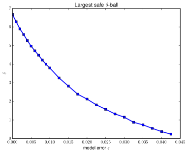
Figure 1: The largest safe ball around the nominal safe action $\mathbf{u}^{*}$ as approximated by $\mathsf{MaxSafeBall}$ for various input model errors $\varepsilon$.

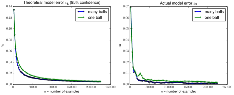
Figure 2: Comparing the theoretical and actual model errors under two safe exploration regimes: (1) random actions chosen from up to 14 safe balls or (2) random actions chosen from a single ball.

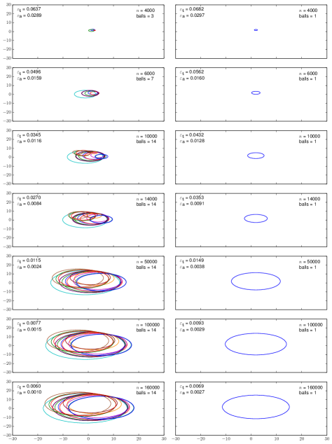
Figure 3: Left column plots show the gradual addition of safe balls (i.e., circles, up to $14$) and growth of each ball. Each plot has $x$ and $y$ axis corresponding to the two control inputs. Each circle within a plot indicates a safe action region where any sequence of $T$ actions is safe. Plots on the right shows gradual growth of a single safe ball.

8 Concluding Remarks

We studied safe exploration for identifying system parameters of a linear Gaussian model. In our approach we defined safety as satisfying linear inequality constraints on the state at each time step of a trajectory. This is motivated by applications involving control of process variables and where violating those constraints may lead to significant negative impacts. We showed how to compute many regions of safe actions when given a nominal safe action. Confined to taking actions within each safe region, any exploration strategy may be applied and theoretical bounds on the approximation quality of an estimated model can be computed online. By computing and exploring within many safe regions, our experiments show we can increase the sample-efficiency of exploration. For future work, we would like to extend safe exploration to not just identify the model as accurately as possible, but to gather just the right kind of transition samples that optimizes the quality of the controller.

Acknowledgments

We like to thank Nevena Lazic, Eehern Wang and Greg Imwalle for useful discussions.

References

- [1] Dario Amodei, Chris Olah, Jacob Steinhardt, Paul Christiano, John Schulman, and Dan Mané. Concrete problems in AI safety. arXiv:1606.06565, 2016.
- [2] Karl-Johan Åström and Torsten Bohlin. Numerical identification of linear dynamic systems from normal operating records. In Theory of Self-Adaptive Control Systems, pages 96–111, Teddington, UK, 1967.
- [3] Karl-Johan Åström and Pieter Eykhoff. System identification: A survey. Automatica, 7(2):123–162, 1971.
- [4] Felix Berkenkamp and Angela P. Schoellig. Safe and robust learning control with Gaussian processes. In European Control Conference (ECC), pages 2496–2501, 2015.
- [5] George E. P. Box, Gwilym Jenkins, Gregory C. Reinsel, and Greta M. Ljung. Time Series Analysis: Forecasting and Control (5th Edition). Wiley, Hoboken, NJ, 2015.
- [6] S. Chen, Billings S. A., and P. M. Grant. Non-linear system identification using neural networks. International Journal of Control, 51:1191–1214, 1990.
- [7] James Demmel. The componentwise distance to the nearest singular matrix. SIAM Journal on Matrix Analysis and Applications, 13:10–19, 1992.
- [8] Jim Gao. Machine learning applications for data center optimization. Google white paper, 2014.
- [9] Javier García and Fernando Fernández. Safe exploration of state and action spaces in reinforcement learning. Journal of Artificial Intelligence Research, 45(1):515–564, 2012.
- [10] Javier García and Fernando Fernández. A comprehensive survey on safe reinforcement learning. Journal of Machine Learning Research, 16(1):1437–1480, 2015.
- [11] Mohammad Ghavamzadeh, Marek Petrik, and Yinlam Chow. Safe policy improvement by minimizing robust baseline regret. In Advances in Neural Information Processing Systems 29 (NIPS-16), pages 2298–2306, Barcelona, Spain, 2016.
- [12] William H. Greene, editor. Econometric Analysis (8th Edition). Pearson, New York, NY, 2018.
- [13] G. Iyengar. Robust dynamic programming. Mathematics of Operations Research, 30(2):1–21, 2005.
- [14] Anayo K. Akametalu, Shahab Kaynama, Jaime Fisac, Melaine N. Zeilinger, Jeremy H. Gillula, and Claire J. Tomlin. Reachability-based safe learning with Gaussian processes. In Proceedings of the IEEE Conference on Decision and Control, pages 1424–1431, Los Angeles, CA, 2014.
- [15] Rogier Koppejan and Shimon Whiteson. Neuroevolutionary reinforcement learning for generalized control of simulated helicopters. Evolutionary Intelligence, 4(4):219–241, 2011.
- [16] Joseph P. LaSelle, editor. The Stability and Control of Discrete Processes. Springer-Verlag, New York, NY, 1986.
- [17] Peter D. Lax, editor. Functional Analysis. Wiley, New York, 2002.
- [18] Lennart Ljung, editor. System Identification: Theory for the User (2nd Edition). Prentice Hall, Upper Saddle River, New Jersey, 1999.
- [19] Mario Milanese and Antonio Vicino. Optimal estimation theory for dynamic systems with set membership uncertainty: An overview. In Mario Milanese, John Norton, Hélène Piet-Lahanier, and Éric Walter, editors, Bounding Approaches to System Identification, chapter 3, pages 5–27. Springer, Boston, MA, 1996.
- [20] Teodor Mihai Moldovan and Pieter Abbeel. Safe exploration in Markov decision processes. In International Conference on Machine Learning, pages 1451–1458, Edinburgh, Scotland, 2012.
- [21] Arnab Nilim and Laurent El Ghaoui. Robust control of Markov decision processes with uncertain transition matrices. Operations Research, 53(1):780–798, 2005.
- [22] Martin Pecka and Tomas Svoboda. Safe exploration techniques for reinforcement learning – an overview. In Modelling and Simulation for Autonomous Systems, pages 357–375, Rome, Italy, 2014.
- [23] Rik Pintelon and Johan Schoukens, editors. System Identification: A Frequency Domain Approach (2nd Edition). Wiley, Hoboken, NJ, 2012.
- [24] Fred C. Schweppe. Recursive state estimation: Unknown but bounded errors and system inputs. IEEE Transactions on Automatic Control, 13:22–28, 1968.
- [25] Yanan Sui, Alkis Gotovos, Joel W. Burdick, and Andreas Krause. Safe exploration for optimization with Gaussian processes. In International Conference on Machine Learning, pages 997–1005, Lille, France, 2015.
- [26] Matteo Turchetta, Felix Berkenkamp, and Andreas Krause. Safe exploration in finite Markov decision processes with Gaussian processes. In Advances in Neural Information Processing Systems 29 (NIPS-16), pages 4312–4320, Barcelona, Spain, 2016.
- [27] Matteo Turchetta, Felix Berkenkamp, Angela P. Schoellig, and Andreas Krause. Safe model-based reinforcement learning with stability guarantees. arXiv:1705.08551, 2017.
- [28] Eric Walter and Hélène Piet-Lahanier. Estimation of parameter bounds from bounded-error data: a survey. Mathematics and Computers in Simulation, 32:449–468, 1990.
- [29] Hans S. Witsenhausen. Sets of possible states of linear systems given perturbed observations. IEEE Transactions on Automatic Control, 13:556–558, 1968.