Memory-constrained Vectorization and Scheduling of Dataflow Graphs for Hybrid CPU-GPU Platforms

Abstract.

The increasing use of heterogeneous embedded systems with multi-core CPUs and Graphics Processing Units (GPUs) presents important challenges in effectively exploiting pipeline, task and data-level parallelism to meet throughput requirements of digital signal processing (DSP) applications. Moreover, in the presence of system-level memory constraints, hand optimization of code to satisfy these requirements is inefficient and error-prone, and can therefore, greatly slow down development time or result in highly underutilized processing resources. In this paper, we present vectorization and scheduling methods to effectively exploit multiple forms of parallelism for throughput optimization on hybrid CPU-GPU platforms, while conforming to system-level memory constraints. The methods operate on synchronous dataflow representations, which are widely used in the design of embedded systems for signal and information processing. We show that our novel methods can significantly improve system throughput compared to previous vectorization and scheduling approaches under the same memory constraints. In addition, we present a practical case-study of applying our methods to significantly improve the throughput of an orthogonal frequency division multiplexing (OFDM) receiver system for wireless communications.

1. Introduction

Heterogeneous multiprocessor platforms are of increasing relevance in the design and implementation of many kinds of embedded systems. Among these platforms, heterogeneous CPU-GPU platforms (HCGPs), which integrate multicore central processing units (CPUs) and graphics processing units (GPUs), have been shown to significantly boost throughput for many applications. System-level performance optimization requires efficient utilization of both CPU cores and GPUs on HCGPs. In embedded system designs, multiple system constraints must be met including memory, latency or cost requirements. Manual performance tuning on a case-by-case suffers from inefficiency and can lead to highly sub-optimal solutions. When system constraints or the target platforms are changed, the designer often needs to repeat the same process, which further reduces development productivity, and increases the chance of introducing implementation errors. Therefore, methods for HCGPs that are based on high-level models, and systematically explore parallelization opportunities are highly desirable.

Dataflow models provide high-level abstractions for specifying, analyzing and implementing a wide range of embedded system applications (e.g., see (Bhattacharyya et al., 2013)). A dataflow graph is a directed graph $G=(V,E)$ with a set of vertices (actors) $V$ and a set of edges $E$. An actor $v\in V$ represents a computational task of arbitrary complexity. An edge $e=(u,v)\in E$ represents a first-in, first-out (FIFO) buffer that stores data values as they are produced by $u$ and consumed by $v$. These data values are called tokens, and represent the basic unit of data that is processed by actors. When an actor fires, it consumes tokens from its input edges, executes its associated task, and produces tokens on its output edges.

Synchronous dataflow (SDF) is a specialized form of dataflow in which the numbers of tokens produced and consumed on each edge are constant across all firings of its source and sink actors (Lee and Messerschmitt, 1987). These two numbers are called the production rate and consumption rate of an edge. Generally, the production rate and consumption rate of an SDF edge can take on any positive integer value. SDF graphs are powerful tools for analyzing and optimizing important system-level metrics, including memory requirements, latency, and throughput. Additionally, SDF graphs naturally expose pipeline, task and data parallelism across distinct actors and distinct firings of the same actor, as illustrated in Figure 1. Pipeline and task parallelism can be exploited by assigning actors on different cores or processors (Figure 1 and 1, while exploitation of data parallelism can be enhanced by vectorization of actors such that different sets of tokens are processed by the same actor concurrently on data-parallel hardware (Figure 1).

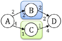
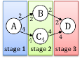
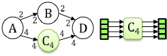
Figure 1. An illustration of parallelism expressed using SDF graphs: (a) task parallelism, (b) pipeline parallelism, (c) data parallelism based on vectorization.

GPUs in HCGPs accelerate computational tasks by supporting large-scale data parallelism with hundreds or thousands of SIMD (single instruction multiple data) processors. GPUs can achieve high throughput gain over CPUs when parallel data is abundant. However, when parallel data is insufficient, GPU performance can be worse compared to CPU cores. For an SDF graph, a sufficient amount of parallel data may not be present to effectively utilize a GPU. In this case, vectorization can be of great utility in improving the degree of exposed data parallelism, and the effective utilization of GPU resources. However, previous research on scheduling and software synthesis from SDF graphs has focused largely on task and pipeline parallelism, therefore providing inadequate support of GPU-targeted design flows. The developments in this paper are intended to address this gap.

In general, the average time required for an actor firing scales differently in terms of the vectorization factor between a CPU and GPU. Additionally, overheads involving interprocessor communication and synchronization can limit or even negate performance gains achieved through vectorization. Thus, effective throughput optimization for HCGPs requires rigorous joint consideration of vectorization and scheduling.

In this paper, we develop integrated vectorization and scheduling (IVS) techniques for software synthesis targeted to HCGPs. These techniques jointly consider vectorization and scheduling for thorough optimization of SDF graphs. We refer to this problem of joint vectorization and scheduling as the SDF vectorization-scheduling throughput optimization (VSTO) problem, or simply as “VSTO”. Our contribution is summarized as follows. First, we formally present the VSTO problem for HCGPs. Second, we develop a set of novel vectorization and scheduling techniques for VSTO under memory constraints. Third, we propose a new scheduling strategy called $\Sigma$-scheduling that is effective for mapping dataflow actors on heterogeneous computing platforms. Finally, we demonstrate our approaches to VSTO by applying them to a large collection of synthetic, randomly-generated dataflow graphs and an Orthogonal Frequency Division Multiplexing (OFDM) receiver.

2. Related Work

SDF throughput analysis under resource constraints using explicit state space exploration has been studied in (Ghamarian et al., 2006). In (Park and Dally, 2010), the authors present a scheduling algorithm for SDF graphs that applies static topological analysis and vectorization to improve SDF throughput and memory usage on shared-memory, multicore platforms. In (Chen and Zhou, 2012), a buffer optimization technique for pipelined, multicore schedules is discussed.

Earlier work on SDF vectorization has focused on throughput optimization for single-processor implementation on programmable digital signal processors, and more recently, on multicore implementation. SDF vectorization techniques to maximize throughput for single-processor implementation were first developed in (Ritz et al., 1993). In (Ko et al., 2008), the authors presented methods to construct vectorized, single-processor schedules that optimize throughput under memory constraints. In (Hsu et al., 2011), the authors presented techniques for maximizing throughput when simulating SDF graphs on multicore platforms. These techniques simultaneously optimize vectorization, inter-thread communication, and buffer memory management. In these works, SIMD architectures are not involved, and vectorization is applied to reduce synchronization overhead and context switching rather than to exploit data-parallelism.

Various studies have targeted automated exploitation of parallelism to map dataflow models onto heterogeneous computing platforms. Design tools that exploit various forms of parallelism using CUDA or OpenCL have been developed in (Ciccozzi, 2013; Lund et al., 2015; Schor et al., 2013). These tools assume that vectorization has been specified by the designer, and map an actor onto a GPU whenever a GPU-accelerated implementation of the actor is available. For such actors, these tools do not take into account the possibility that CPU-targeted execution may be more efficient. In (Zaki et al., 2013), SDF graphs are automatically vectorized, transformed to single-rate SDF graphs, and then scheduled using Mixed-Integer Programming techniques. However, this approach does not take memory constraints into account. Intuitively, a single-rate SDF graph is one in which all actors are fired at the same average rate. This concept is discussed in more detail in Section 3.

When SDF graphs are converted to single-rate graphs, they can be scheduled in the same way that task graphs are scheduled in programming environments such as StarPU (Augonnet et al., 2011), FastFlow (Goli et al., 2012), and OmpSS (Duran et al., 2011). These environments support run-time task graph scheduling and parallelization on hybrid CPU-GPU platforms. StarPU, for example, uses the Heterogeneous Earliest Finish Time (HEFT) heuristic to schedule tasks on HCGPs. However, these programming models cannot directly be applied to multirate SDF graphs; a designer must manually vectorize the graph and convert it to a single-rate SDF graph before working with it in such environments. In addition to requiring such manual transformation, this process limits the flexibility in vectorization and scheduling for SDF execution, which can lead to inefficient memory usage and execution time performance.

Dataflow models can be used at arbitrary levels of abstraction in computing systems, and hence compilation optimization of dataflow programs is also investigated at various levels of abstraction. For example, the works in (Udupa et al., 2009; Hagiescu et al., 2011) focus on improving the throughput of GPU kernels that are represented by dataflow graphs. The aim of those works is to generate high-performance GPU kernel code through better utilization of on-device resources. In contrast, the methods introduced in this paper focus on optimizing the mapping of coarse-grain, system-level dataflow models onto CPU-GPU platforms, where each actor can encompass a computational task of arbitrary complexity, and can encapsulate one or multiple kernels.

In this work, we go beyond the previous works by jointly considering SDF vectorization and scheduling for HCGPs under memory constraints. To our knowledge, our work is the first to take memory constraints into account in the context of SDF vectorization and scheduling for heterogeneous computing platforms. Our methods are not restricted to single-rate SDF graphs, and are capable of deriving efficient, memory-constrained vectorization configurations. The techniques in this paper are developed in the DIF-GPU Framework, which was presented in (Lin et al., 2016). DIF-GPU incorporates techniques for minimizing runtime overhead through compile-time scheduling and incorporation of carefully-designed protocols for interprocessor communication.

3. Background

The HCGPs that we target in this paper consist of one multi-core CPU and one GPU each. This class of multicore architectures is widely used in embedded systems. In our targeted class of HCGPs, we refer to the CPU as the host, as it controls overall execution flow and manages the associated GPU, and we refer to the GPU as the device. The device receives instructions and data from the host.

Additionally, in the target architecture, there exists a context transfer overhead when an application’s execution path switches between CPU cores and a GPU. This overhead can include the time for interprocessor communication and synchronization, context switching, and transferring data from one memory address to another. Although most existing embedded HCGPs provide shared physical memory, this context transfer overhead can still be significant, and in general varies from one architecture / application to another (Gregg and Hazelwood, 2011). We refer to such context transfer overhead as host-to-device (H2D) or device-to-host (D2H) context transfer, depending on the direction.

Given an SDF graph $G=(V,E)$ and an actor $v\in V$, we denote the sets of input and output edges of $v$ as $\mathit{in}(v)$ and $\mathit{out}(v)$, respectively. Given an edge $e\in E$, we denote the source and sink actors of $e$ by $\mathit{src}(e)$ and $\mathit{snk}(e)$, respectively. We denote as $\mathit{prd}(e)$ the number of tokens produced onto $e$ by each firing of $\mathit{src}(e)$, and similarly, we denote as $\mathit{cns}(e)$ the number of tokens consumed from $e$ by each firing of $\mathit{snk}(e)$.

Signal processing systems represented as SDF graphs are often required to be executed indefinitely — that is, iterated through a number of iterations for which no useful bound is known in advance. To support such indefinite execution, the concepts of consistency and periodic schedules in SDF graphs are important (Lee and Messerschmitt, 1987). An SDF graph is consistent if it has a periodic schedule, which is a sequence of actor executions that does not deadlock, fires each actor at least once, and produces no net change in the number of tokens on each edge. Consistent SDF graphs can be executed indefinitely with finite buffer memory requirements. Furthermore, for each actor $v\in V$ in a consistent SDF graph $G=(V,E)$, there is a unique repetition count $q(v)$, which gives the minimum number of firings of $v$ in a periodic schedule. We call a set of actor firings in which each actor $v$ fires exactly $q(v)$ times an iteration of $G$. Figure 2 shows an SDF graph example, where each repetition count is denoted as $<q(v)>$ above the corresponding actor $v$. In this example, $\mathit{prd}(e_{AB})=1$, $\mathit{cns}(e_{AB})=2$, $q(A)=2$, and $q(C)=7$.

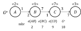
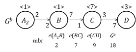
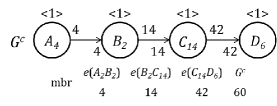
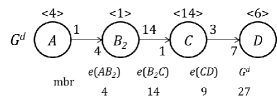
Figure 2. An example of vectorization and minimum buffer requirements. (a) Original graph. (b) Actor-level Vectorization of $A$ by 2. (c) Graph-level Vectorization with $\beta=2$. (d) Actor-level Vectorization of $B$ by 2.

If $q(v)=1$ for every actor $v\in V$, then $G$ is called a single-rate SDF graph, as shown in Figure 2. Because each actor needs to fire only once to complete an iteration of $G$, single rate SDF graphs can be scheduled the same way as task graphs (e.g., see (Zaki et al., 2013)). In a task graph, nodes represent computational tasks, and edges represent dependencies associated with pairs of nodes without any specific data structure implied for inter-actor communication. A wide variety of algorithms have been developed for scheduling task graphs onto multiprocessor systems (e.g., see (Sriram and Bhattacharyya, 2009)).

For implementation of $G$, we assume a static buffer allocation model, where we allocate a FIFO buffer of fixed, finite size (“buffer bound”) $\mathit{buf}(e)$ for each edge $e\in E$. When an actor $v$ fires, it must satisfy (1) for each edge $e_{i}\in\mathit{in}(v)$, $e_{i}$ contains at least $\mathit{cns}(e_{i})$ tokens, and (2) for each edge $e_{o}\in\mathit{out}(v)$, $e_{o}$ contains no more than $(\mathit{buf}(e_{o})-\mathit{prd}(e_{o}))$ tokens. When this condition is met, the actor is said to be bounded-buffer fireable, and SDF graph execution following this rule is called bounded-buffer execution.

The minimum buffer requirement for an SDF graph $G$, $\mathit{mbr}(G)$, is the minimum over all periodic schedules of the amount of memory (in units of tokens) required to implement the dataflow edges in a given graph (see (Stuijk et al., 2006)). A lower bound $\mathit{mbr}(e)$ on the minimum buffer requirement for a delayless SDF edge $e$ can be determined by

(1) $$\mathit{mbr}(e)=\mathit{prd}(e)+\mathit{cns}(e)-\mathit{gcd}(\mathit{prd}(e),\mathit{cns}(e)),$$

where $\mathit{gcd}$ represents the greatest common divisor operator (Bhattacharyya et al., 1996). The lower bound of $\mathit{mbr}(G)$ is the sum of $\mathit{mbr}(e)$ over all edges: $\mathit{mbr}(G)=\sum_{v\in V}\mathit{mbr}(e)$. Although this lower bound is not always achievable, it is achievable for the dataflow graphs in Figure 2.

We represent the individual processors in the target multiprocessor platform as $P=\{p_{1},p_{2},\ldots,p_{N}\}$, where $p_{1},p_{2},\ldots,p_{N-1}$ represent the available CPU cores, and $p_{N}$ represents the GPU. When scheduling $G$ onto the platform, actor firings are assigned to processors to be executed. In this context, we say that an actor $v\in V$ is mapped onto processor $p\in P$ if all firings of $v$ are assigned to execute on $p$.

As mentioned in Section 2, we assume in this paper that the input SDF graphs for vectorization and software synthesis are acyclic. Cycles in synchronous dataflow models may impose complex constraints on what vectorization degrees are valid for actors (Ritz et al., 1993). Furthermore, cycles introduce complex trade-offs between code size and buffer memory minimization in SDF graphs, which are also relevant to memory-constrained vectorization problems (e.g. see (Bhattacharyya et al., 1996)). Third, acyclic SDF graphs encompass a broad class of important signal processing applications, so techniques for this class have significant practical relevance (Bhattacharyya et al., 1996). Currently in our framework, we assume that actor vectorizations are constrained only by memory, and not by cycles in the input graph. Investigating vectorization with topological constraints caused by cycles is an interesting direction for future work.

4. Problem Formulation

In this section, we formally define the VSTO problem for HCGPs. We begin by defining the concept of actor-level vectorization. Given a consistent SDF graph $G=(V,E)$, and an actor $v\in V$, the vectorization of $v$ by a vectorization degree (VCD) $b$ is defined as a transformation of $G$ that involves the following set of operations: (1) replacing $v$ by $v_{b}$, where firing $v_{b}$ is equivalent to $b$ consecutive firings of $v$; (2) replacing each edge $e_{i}\in\mathit{in}(v)$ by an edge $e_{i}^{\prime}$ such that $\mathit{cns}(e_{i}^{\prime})=b\times\mathit{cns}(e_{i})$ and $\mathit{prd}(e_{i}^{\prime})=\mathit{prd}(e_{i})$; and (3) replacing each edge $e_{o}\in\mathit{out}(v)$ by an edge $e_{o}^{\prime}$ such that $\mathit{prd}(e_{o}^{\prime})=b\times\mathit{prd}(e_{o})$ and $\mathit{cns}(e_{i}^{\prime})=\mathit{cns}(e_{i})$. We refer to the actor $v_{b}$ as the $b$-vectorized actor of $v$, and the transformed graph that results from the vectorization operation as $\mathit{vect}(G,v,b)$. For example, in Figure 2, $G^{b}=\mathit{vect}(G^{a},A,2)$. The definition of vectorization that we adopt here corresponds to a dataflow graph transformation that is consistent with the vectorization concept introduced by Ritz et al. (Ritz et al., 1993), as opposed to the aggregation of basic operations that corresponds to vectorization in compilers for procedural programming languages.

If $G$ is a consistent, acyclic SDF graph, then $\mathit{vect}(G,v,b)$ is also consistent for any $v\in V$, and any positive integer $b$. However, in this work, we restrict the set of allowable vectorization degrees to the set $\mathit{alwb}(G,v)$, which is defined as

(2) $$\mathit{alwb}(G,v)=\{n\in\{1,2,\ldots\}\mid(n\mathrm{\ is\ a\ factor\ of\ }q(v))\mathrm{\ or\ }(n\mathrm{\ is\ a\ multiple\ of\ }q(v))\}.$$

Equation 2 refers specifically to positive integer factors and multiples. For example, if $q(v)=8$, then $\mathit{alwb}(G,v)=\{1,2,4,8,16,24,\ldots\}$. Vectorization of an actor $v$ that is restricted to $\mathit{alwb}(G,v)$ enables fast derivation of repetition counts for $G^{\prime}=\mathit{vect}(G,v,b)$, which in turn facilitates incremental vectorization techniques, where actors are selected for vectorization one at a time according to specific greedy criteria. In particular, if $b$ is a factor of $q(v)$, then $q(G^{\prime},v)=q(G,v)/b$ , while the repetition counts of all other actors are unchanged. Similarly, if $b$ is a multiple of $q(v)$, then $q(G^{\prime},v)=1$, while for any other actor $u\neq v$, $q(G^{\prime}u)=bq(G,u)/q(G,v)$. In Section 5, we discuss specific techniques for incremental vectorization that apply these forms of repetition count updates.

On HCGPs, vectorized actors can exploit SIMD processors such as GPUs to execute multiple firings of the same actor in parallel. Note that although parallel processing of tokens cannot in general be applied easily to stateful actors, vectorization may still benefit dataflow execution by reducing overheads associated with inter-processor communication, synchronization and context switching. In the presence of memory constraints, there are limits to the amount of vectorization that can be applied. For example, as we can see in Figure 2, vectorizing $A$ (Fig. 2) and vectorizing $B$ (Fig. 2) by 2 results in different increases to the minimum buffer requirement.

To represent SDF graphs with vectorized actors and their relationships with the original graphs, we define vectorized SDF graphs (VSDFs) as follows.

Definition 4.1.

Suppose that $G=(V,E)$ is a consistent SDF graph, $b_{v}\in\mathit{alwb}(v,G)$ is a VCD for each $v$, and $B=\{(v,b_{v})\mid v\in V\}$. Then the $B$-vectorized SDF graph of $G$ is defined as $G_{B}=(V_{B},E_{B})$, where (1) each $v_{B}\in V_{B}$ is the $b_{v}$-vectorized actor of $v$, (2) each edge $e_{B}=(x_{B},y_{B})$ in $G_{B}$ is derived from the corresponding edge $(x,y)\in E$, and (3) for each $e_{B}=(u_{B},v_{B})\in E_{B}$, $\mathit{prd}(e_{B})=b_{u}\times\mathit{prd}(e)$, and $\mathit{cns}(e_{B})=b_{v}\times\mathit{cns}(e)$, where $e=(u,v)$.

The vectorized graph $G_{B}$ is an SDF graph. We define a restricted form of vectorization, called graph-level vectorization (GLV), in which a common “repetitions vector multiplier” $\beta\in\{1,2,\ldots\}$ is used for all actors in the input graph. That is, $b_{v}=\beta\times q(G,v)$ for all $v\in V$. In this context, we refer to $\beta$ as the graph vectorization degree (GVD). Under GLV , $G_{B}$ is a single-rate SDF graph. However, vectorization does not need to be confined to GLV. We refer to this more general form of vectorization, as actor-level vectorization (ALV). For example, Figure 2 shows the vectorized graph that corresponds to Figure 2 with GLV and $\beta=2$. Figure 2 shows the vectorized graph that results from applying ALV to Figure 2 with $b_{B}=2$.

As discussed in Section 2, the conventional approach to solving VSTO involves 3 steps: (1) the designer or design tool sets the GVD based on memory constraints, (2) converts the SDF graph into a single-rate SDF graph using GLV, and (3) generates a schedule using task graph scheduling methods. Compared to ALV, GLV can require significantly larger buffers (see Figure 2). The vectorization methods that we present in this paper go beyond these conventional approaches by considering general ALV solutions instead of being restricted only to GLV solutions.

For multiprocessor scheduling of ALV solutions, we introduce in this work a general scheduling strategy, which is suitable for HCGPs, and can loosely be viewed as a variant of the list scheduling strategy. This variant is adapted for memory-constrained, multiprocessor mapping of transformed graphs that result from ALV. This strategy is a static scheduling strategy that operates using compile-time estimates of actor execution times. The general strategy is defined as follows.

Definition 4.2.

Given a consistent SDF graph $G=(V,E)$, and a multiprocessor target architecture with a set of processors $P$, the $\Sigma$-scheduling strategy (1) statically assigns each actor $v\in V$ to a processor $p\in P$, (2) statically determines a buffer bound $\mathit{buf}(e)$ for each edge $e\in E$, and (3) iteratively selects a bounded-buffer firable actor to fire on its assigned processor $p$ as soon as $p$ has completed all executions. An algorithm that conforms to this scheduling strategy completes when all actors in $G$ have been scheduled using the iterative process of Step (3).

The $\Sigma$-scheduling strategy is closely related to the $\Omega$-scheduling strategy, which was introduced in (Hsu et al., 2011). Both the $\Sigma$ and $\Omega$ strategies satisfy Parts (1) and (2) of Definition 4.2; the main difference is that with respect to Part (3), $\Sigma$-scheduling maps actors onto a finite number of processors, while $\Omega$-scheduling assumes an unlimited number of processors. Additionally, in our application of $\Sigma$-scheduling, we perform ALV to construct the input graph to the strategy. In contrast, $\Omega$-scheduling in (Hsu et al., 2011) is applied to the original (unvectorized) SDF graph.

To determine the buffer bounds $\{\mathit{buf}(e)\}$ in $\Sigma$-scheduling, we apply the $\Omega$-buffering technique defined in (Hsu et al., 2011). This technique derives the buffer bounds by applying $\Omega$-scheduling, and determining the buffer bounds to be equal to the corresponding buffer sizes $\{\mathit{buf}(e)\}$ that result from $\Omega$-scheduling. We refer to the buffer bound $\mathit{buf}(e)$ for each edge $e$ that is computed in this way as the $\Omega$ buffer bound for $e$. It is shown that $\Omega$-buffering sustains maximum throughput for SDF graphs under $\Omega$ scheduling (Hsu et al., 2011) so that imposing these bounds imposes no theoretical limitation on throughput. Given an SDF graph $G=(V,E)$, we denote by $\Omega_{\mathit{buf}}(G)$ the total buffer memory cost for $G$ as determined by $\Omega$-scheduling: $\Omega_{\mathit{buf}}(G)=sum_{e\in E}(\mathit{buf}(e))$.

Definition 4.3.

Suppose that $G=(V,E)$ is a consistent SDF graph, $b_{v}\in\mathit{alwb}(v,G)$ is a VCD for each $v$, $B=\{(v,b_{v})\mid v\in V\}$, $S_{B}$ is a periodic schedule for the $B$-vectorized graph $G_{B}$, and $T(S_{B})$ is an estimate of the time required to execute a single iteration of $S_{B}$. Then from the fundamental properties of periodic SDF schedules (Lee and Messerschmitt, 1987), we can derive a unique positive integer $J(S_{B},G)$, which we call the blocking factor of $S_{B}$ relative to $G$, such that $S_{B}$ executes each $v\in V$ exactly $(J(S_{B},G)\times q(G,v))$ times. In this context, we define the relative throughput of $S_{B}$ or the throughput of $S_{B}$ relative to $G$ by the quotient $J(S_{B},G)/T(S_{B})$. This metric gives the average number of iterations of the original (unvectorized) SDF graph that is executed per unit time by the schedule $S_{B}$.

As an example, in Figure 2, executing one iteration of $G^{b}$, $G^{c}$ or $G^{d}$ is equivalent to executing two iterations of $G^{a}$. Thus, $J(S_{B},G^{b})=J(S_{B},G^{c})=J(S_{B},G^{d})=2$.

Intuitively, vectorization improves relative throughput when $T(S_{B})<J(S_{B})\times T(S)$, where $S$ is the best available minimal-periodic (unvectorized) schedule for $S$. Such efficiency in the vectorized execution time $T(S_{B})$ can be achieved due to improved utilization of processing resources under carefully-optimized GLV and ALV configurations.

A limitation of the vectorization techniques developed in this paper is that they may increase latency, and thus, they may not be suitable for implementations in which latency is a critical performance metric. However, it is envisioned that the methods developed in this paper provide a useful foundation that can be built upon for latency-aware vectorization. Investigating adaptations of these methods to take latency constraints into account is an interesting direction for future work.

Based on the definitions introduced in this section, we formulate the VSTO problem as follows.

Definition 4.4.

Let $G=(V,E)$ be a consistent SDF graph, and $P=\{p_{1},p_{2},\ldots,p_{N}\}$ be the set of processors in an HCGP, where $p_{1},p_{2},\ldots,p_{N-1}$ represent the CPU cores, and $p_{N}$ represents the GPU. Given a total memory budget $M$ (a positive integer), the vectorization-scheduling throughput optimization problem, or VSTO problem associated with $G$ and $P$ is the problem of finding a set $B$ of vectorization degrees, and a schedule $S_{B}$ for $G_{B}=(V_{B},E_{B})$ such that the throughput of $S_{B}$ relative to $G$ is maximized subject to $\Omega_{\mathit{buf}}(G_{B})\leq M$.

We refer to a set of ordered pairs $C=\{(v,c_{v})\mid(v\in V)\mathrm{\ and\ }(c_{v}\in\mathit{alwb}(G,v))\}$ as an ALV configuration for $G$. Note that if an actor is not represented within a given ALV configuration (i.e., it does not appear as the first element of any ordered pair in the set), then the actor is assumed to be unvectorized (equivalent to a vectorization degree of $1$). Thus, the VSTO problem can be thought of as the problem of jointly determining an ALV configuration $B$ together with a schedule for $G_{B}$ such that the resulting schedule optimizes throughput subject to a given buffer memory constraint $M$.

The vectorization formulation and techniques developed in this paper assume that each SDF edge (FIFO buffer) is implemented in a separate block of memory. Various techniques have been developed in recent years to share memory efficiently among edges in multirate SDF graphs (e.g., see (Tripakis et al., 2013; Desnos et al., 2015)). Extending the techniques in this paper to incorporate such memory sharing techniques is a useful direction for future work.

5. Vectorization and Scheduling with Memory Constraints

In this section, we develop three main heuristics, called Incremental Actor Vectorization (IAV), $N$-candidates IAV, and Mapping-Based Devectorization, for the VSTO problem. These three heuristics can be viewed as “peers” in the sense that any one of them may be the preferable choice for a given application. Thus, the designer or a design tool can apply all three of these complementary methods and select the best result for a given application. This is how we have integrated the three heuristics in our DIF-GPU software framework. More details on the integration with software synthesis and associated experimental results are discussed in Section 6 and Section 7.

5.1. Incremental Actor Vectorization

In this section, we define a general approach for searching the space of ALV configurations that is based on selecting and vectorizing actors one at a time using some specific greedy criteria. We refer to this general approach as Incremental Actor Vectorization (IAV). Each iteration of IAV, called an IAV iteration, involves the selection and vectorization of a single actor. This results in a sequence of intermediate vectorized graphs, $I_{1},I_{2},\ldots,I_{N}$, where $I_{i}$ is the transformed graph that results from IAV iteration $i$, and $N$ is the total number of iterations before IAV terminates. The approach is incremental in both the dimensions of actors and vectorization degrees — that is, each IAV iteration selects a single actor $v$, and increases its vectorization degree to the next highest element of $\mathit{alwb}(G,v)$. Given an actor $v$ that has an associated vectorization degree $b_{v}$, we refer to this process of replacing $b_{v}$ with the next highest element $\mathit{min}(x\in\mathit{alwb}(v)\mid x>b_{v})$ as stepping up the vectorization of $v$ or just “stepping up $v$”.

In IAV, we define a “score” function to guide the vectorization process. At each algorithm iteration, IAV selects an actor that has the highest score among all actors whose stepping up would not result in a violation of the given memory budget $M$. Analogous to how different priority functions can be used to select tasks in multiprocessor list scheduling (e.g., see (Sriram and Bhattacharyya, 2009)), different score functions can be used to apply different ALV criteria in IAV. This contributes to a novel design space for development of integrated vectorization and scheduling techniques.

The specific score functions that we experiment with in this work first apply $\Sigma$-scheduling to generate a schedule $\mu(i)$ of the current $I_{i}$ (intermediate vectorized graph) onto the target HCGP $P$, and then use a specific metric to estimate the potential “gain” of each candidate stepping up operation relative to the processor assignment associated with $\mu(i)$. Given a schedule $S$ returned by $\Sigma$-scheduling, we define the associated processor assignment associated with $S$ and dataflow graph $G=(V,E)$ as the function $\mathit{mp}_{S}\mathrel{\mathop{\mathchar 58\relax}}V\rightarrow P$ such that for each $v\in V$, $\mathit{mp}_{S}(v)$ gives the processor to which actor $v$ is mapped according to $S$. The initial schedule $\mu(0)$ is derived by applying $\Sigma$-scheduling to the input (unvectorized) graph for IAV.

Algorithm 1 shows a pseudocode description of the IAV approach that employs this mapping-based method of score function formulation. In the remainder of this paper, we refer to the mapping-based form of IAV shown in Algorithm 1 as “$\Sigma$-IAV”.

Function $\textnormal{{incrementalVectorize}}(G,P,M)$

       initialize $\textnormal{{$\mathit{configs}$}}=\emptyset$, $G_{B}=G$, $B=\{(v,1)|v\in V\}$ ;

       while $\textnormal{{memSize}}(G_{B})\leq M$ do

             $\textnormal{{$\mathit{mp}$}}=\textnormal{{generateMapping}}(G_{B},P)$;

             $v^{*}=\operatorname*{\arg\!\max}_{v\in V}\textnormal{{score}}(B,\textnormal{{$\mathit{mp}$}},v)$;

             $B(v^{*})=\textnormal{{nextVCD}}(v^{*},b_{v^{*}})$ ;

             $G_{B}=\textnormal{{vectorize}}(G,B)$ ;

             if $\textnormal{{memSize}}(G_{B})\leq M$ then

                   $\textnormal{{$\mathit{configs}$}}=\textnormal{{$\mathit{configs}$}}\cup\{(B,\textnormal{{$\mathit{mp}$}})\}$ ;

                  

             end if

            

       end while

      return $\operatorname*{\arg\!\max}_{\textnormal{{$\mathit{c}$}}\in\textnormal{{$\mathit{configs}$}}}\textnormal{{throughput}}(G,\textnormal{{$\mathit{c}$}})$

ALGORITHM 1 Integrated vectorization and mapping using $\Sigma$-IAV.

In Algorithm 1, generateMapping is a placeholder for any $\Sigma$-scheduling technique that is applied to map a given intermediate vectorized graph onto the targeted heterogeneous platform $P$. In our implementation of $\Sigma$-IAV, we employ a specific $\Sigma$-scheduling technique called Incremental Actor Re-assignment (IAR) as the generateMapping function. The IAR technique is discussed further in Section 4. The function $\mathit{nextVCD}(v,b_{v})$ gives smallest element of $\mathit{alwb}(v)$ that exceeds $b_{v}$.

The function throughput referenced in Algorithm 1 represents a placeholder for any function that is used to estimate the throughput of a mapping that is generated by generateMapping for an intermediate vectorized graph. In our implementation of $\Sigma$-IAV, we employ an efficient simulation-based approach for this kind of throughput estimation. This simulation approach is discussed further in Section 5.5. In general, heuristic-based mapping techniques, including our techniques, do not guarantee an optimal scheduling. It is therefore possible for the throughput to get worse during incremental vectorization. For this reason, we assess the throughput of each computed configuration and then select a configuration that results in the best throughput.

We formulate and experiment with two specific score functions in this work. We refer to these score functions as time-saving (TMSV) and time-saving-per-byte (TMSVPB). The TMSV score for actor $v$ during IAV iteration $i$ is defined as largest adjusted execution time reduction achievable (across all processors in $P$) when stepping up $v$. This “adjusted” time reduction is computed relative to the execution of $v$ on $\mathit{mp}_{\mu(i)}(v)$, and is normalized by the vectorization degree. The units of this adjusted time reduction are thus “seconds per unit of vectorization”. This score can be expressed as:

(3) $$\mathit{tmsv}(v,i)=\max_{p\in P}(\frac{t(v,b,\mathit{mp}_{\mu(i)}(v))}{b}-\frac{t(v,b^{\prime},p)}{b^{\prime}}),$$

where $b$ is the current VCD of $v$ (in IAV iteration $i$), and $b^{\prime}\in\mathit{alwb}(v)$ is the VCD that would result from stepping up $v$. For a given actor $v$, vectorization degree $b\in\mathit{profiled}(v)$, and processor $p\in P$, $t(v,b,p)$ gives the profiling-derived estimate for the execution time of $v$ on $p$ with vectorization degree $b$.

Here, we use “profiling” as a general term that encompasses any method for deriving a compile-time estimate for the execution time of a vectorized actor execution. The specific approach to profiling that we use in our experiments is discussed in Section 6.

Figure 3 shows a simple example of vectorization using the TMSV score function. The table in this figure provides analytical models, in terms of the vectorization degree $v$, that are used to derive the profiling function $t$. For example, the models estimate that actor $A$ requires approximately $(0.5\times v)$ units of time to execute.

The IAV process begins with an unvectorized graph and an initial mapping where all actors are mapped to the CPU core. In the first IAV iteration ($i=0$) shown in Figure 3, $A$ has the largest TMSV score, so it is selected, and a new mapping is generated based on the VCDs. In the second iteration, $B$ has the largest TMSV score, so $B$ is vectorized (stepped up), and the mapping is updated again. This process continues until no more vectorization operations can be carried out without exceeding the memory budget $M$.

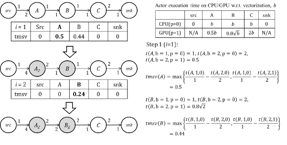
Figure 3. A simple example to illustrate $\Sigma$-IAV using the TMSV score function.

Under memory constraints, we expect that it will be more useful to consider the increase in buffer requirements when selecting actors for ALV. This motivates our formulation of the TMSVPB score function. Here, “PB” stands for “per byte.” This memory-aware score function can be formulated as:

(4) $$\mathit{tmsvpb}(v,i)=\max_{p\in P}(\frac{t(v,b,\mathit{mp}_{\mu(i)}(v))/b-t(v,b^{\prime},p)/b^{\prime}}{\Omega_{\mathit{buf}}(G_{B^{\prime}})-\Omega_{\mathit{buf}}(G_{B(i)})+\epsilon}),$$

where $B(i)$ represents the current ALV configuration in ILV iteration $i$, and $B^{\prime}=B(i)-\{(v,b)\}+\{(v,b^{\prime})\}$ represents the candidate configuration that results from stepping up $v$. $\epsilon$ is a small constant to avoid division by 0 when $\Omega_{\mathit{buf}}(G_{B^{\prime}})=\Omega_{\mathit{buf}}(G_{B(i)})$ . Thus, the TMSVPB function favors actors whose vectorization results in throughput improvement without excessive increase in buffer requirements.

5.2. $N$-Candidates IAV

Our proposed $\Sigma$-IAV approach has two drawbacks — (1) it selects only one actor at each step, and (2) with the TMSV and TMSVPB score functions, the selections are based primarily on actor execution times, and do not take into account the SDF graph topology. We alleviate the first drawback by storing multiple vectorized-graph candidates to consider in each IAV iteration following the very first iteration. In particular, we store $N$ candidate graphs that provide the highest throughput when processed by $\Sigma$-scheduling. Here, $N$ is a parameter that can be controlled by the designer or tool developer.

The second drawback can be addressed by applying $\Sigma$-scheduling to optimize throughput over each actor for every candidate graph. That is, for each candidate graph $Y$ that is stored, and each actor $v$, we apply $\Sigma$-scheduling to the transformed graph that results from stepping up $v$ in $Y$. We then take the best result from all of these $\Sigma$-scheduling-based evaluations to determine the vectorization operation that is to be applied in the associated IAV iteration. This approach results in some increase in complexity, but has the potential to perform significantly more thorough optimization at a relatively high level of design abstraction.

We refer to this modified $\Sigma$-IAV approach as $N$-candidates IAV. Algorithm 2 provides a pseudocode description of $N$-Candidates IAV. Here, the notation $c.1$ denotes the first element of the ordered pair $c$, and $\mathit{configs}[1\mathrel{\mathop{\mathchar 58\relax}}N]$ denotes the list that consists of the first $N$ elements of the list $\mathit{configs}$. The function $\mathit{visited}(B^{\prime})$ tests whether the vectorization configuration $B^{\prime}$ has been examined before during operation of the algorithm.

Function $\textnormal{{nCandidatesVectorize}}(G=(V,E),P,M,N)$

       initialize $B=\{(v,1)|v\in V\}$, $\textnormal{{$\mathit{mp}$}}=\textnormal{{generateMapping}}(G,P)$, $\textnormal{{$\mathit{configs}$}}=\{(B,\textnormal{{$\mathit{mp}$}})\}$, $\textnormal{{$\mathit{flag}$}}=\textnormal{{$\mathit{true}$}}$ while $\textnormal{{$\mathit{flag}$}}=\textnormal{{$\mathit{true}$}}$ do

             $\textnormal{{$\mathit{flag}$}}=\textnormal{{$\mathit{false}$}}$ ;

             foreach $\textnormal{{$\mathit{c}$}}\in\textnormal{{$\mathit{configs}$}}$ do

                   foreach $v\in V$ do

                         $B^{\prime}=\textnormal{{$\mathit{c}$}}.1-\{(v,b_{v})\}\cup\{(v,\textnormal{{nextVCD}}(v,b_{v})\}$;

                         if $(\textnormal{{visited}}(B^{\prime})=\textnormal{{$\mathit{false}$}})\mathit{and}(\Omega_{\mathit{buf}}(G_{B^{\prime}})\leq M)$ then

                               $\textnormal{{$\mathit{mp}$}}=\textnormal{{generateMapping}}(G_{B^{\prime}},P)$;

                               $\textnormal{{$\mathit{configs}$}}=\textnormal{{$\mathit{configs}$}}\cup\{(B^{\prime},\textnormal{{$\mathit{mp}$}})\}$ ;

                               $\textnormal{{$\mathit{flag}$}}=\textnormal{{$\mathit{true}$}}$, $\textnormal{{visited}}(B^{\prime})=\textnormal{{$\mathit{true}$}}$ ;

                              

                         end if

                        

                   end foreach

                  

             end foreach

            sortByThroughput ($\mathit{configs}$);

             $\textnormal{{$\mathit{configs}$}}=\textnormal{{$\mathit{configs}$}}[1\mathrel{\mathop{\mathchar 58\relax}}N]$

       end while

      return $\operatorname*{\arg\!\max}_{\textnormal{{$\mathit{c}$}}\in\textnormal{{$\mathit{configs}$}}}\textnormal{{throughput}}(G,\textnormal{{$\mathit{c}$}})$

ALGORITHM 2 A pseudocode description of $N$-candidates IAV.

As with our implementation of $\Sigma$-IAV, we employ in our implementation of $N$-candidates IAV the IAR technique (Section 4) as the generateMapping function. Similarly, our implementation of $N$-candidates IAV incorporates the simulation-based throughput estimation technique that is discussed in Section 5.5. This estimation technique corresponds to the function called throughput in Algorithm 2.

Intuitively, $N$-candidates IAV is a greedy method that tries to avoid unsatisfactory search paths by retaining multiple intermediate vectorized graphs during each IAV iteration. Larger values for the parameter $N$ allow more extensive design space exploration at the cost of greater running time. When $N=1$, $N$-candidates IAV reduces to IAV with the score function being the estimated throughput (“throughput”) of the transformed graph that results from the selected vectorization operation. In our implementation of $N$-candidates IAV, we estimate throughput using simulation. This simulation approach is discussed further in Section 5.5. In Algorithm 2, $\textnormal{{throughput}}(G,\mathit{c})$ represents the estimate of throughput that is derived in this way for a given intermediate vectorized graph $G$ that is based on ALV configuration $\mathit{c}$.

Other score functions can be used in $N$-candidates IAV other than throughput. However, in our experiments, we found that among TMSV, TMSVPB, and throughput, the throughput score function produces the best results. Investigation of other score functions in this context is an interesting direction for future work. In our experiments, we use $N=|V|$ as the number of candidates to be stored. We select $N=|V|$ so that NIAV keeps a number of candidates that scales with the number of actors in the dataflow graph while keeping analysis time manageable.

IAR, IAV and NIAV are all greedy-algorithm motivated heuristics based on an evaluation metric (score function) to select vectorization choices at each step. Investigation of other types of heuristics to further improve vectorization is a useful direction for future work.

5.3. Mapping-Based Devectorization

$N$-candidates IAV is an incremental vectorization method that starts with an unvectorized graph, and gradually increases the VCDs of selected actors. In some cases, it may be advantageous to also consider decreasing VCDs during the optimization process. Such decreasing of VCDs can be useful to reduce memory consumption associated with selected actors so that memory can be dedicated to groups of other actors that provide greater throughput benefit through vectorization. A specific form of decrease that we consider in this section is devectorization, where an actor with VCD $b>1$ is transformed to have no vectorization (VCD of unity).

Figure 4(a) shows an example of this kind of scenario. Here, $S$ (source), $K$ (sink), $F$ (fork), and $C$ (combine) are computationally simple actors without potential for GPU acceleration, and only very limited potential for speedup through CPU-based vectorization. On the other hand, actors $A_{1},A_{2},A_{3},A_{4}$ have GPU-accelerated versions with significant throughput gain. In this case, however, the overall throughput gain is limited by the slowest of the four $A_{i}$s so that incrementally vectorizing individual $A_{i}$s does not directly impact throughput gain.

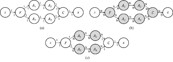
Figure 4. An example that illustrates the utility of devectorization. (a) The original graph. (b) The graph with $\mathrm{GVD}=N$ applied. (c) The graph with devectorization applied to all CPU-mapped actors — $C,F,K,S$.

To provide memory efficient vectorization in which this kind of scenario is of dominant concern, we propose another vectorization method called Mapping-Based Devectorization (MBD). In contrast with ALV-based incremental vectorization, MBD applies GLV to first vectorize all vectorizable actors, and then performs devectorization on the transformed graph derived from GLV. MBD is useful in devectorizing actors that have relatively low CPU-based performance gain through vectorization, and in jointly considering vectorization improvements produced by groups of actors.

MBD performs GLV, generates a processor assignment $A$, and then evaluates for devectorization each actor that is mapped to a CPU core in $A$. If a given devectorization operation does not reduce the original throughput by a pre-defined threshold $r$, the actor is devectorized. In our experiments, we set the threshold $r$ empirically by experimenting with different values of $r$. We found in our experiments that $r=0.95$ achieves the maximum throughput gain for MBD (see Section 6) on the same set of random graphs. The optimal choice of $r$ may change for a different set of graphs. Alternatively, $r$ can be customized for a given graph by performing a search (such as a binary search) to optimize this parameter.

Although the MBD algorithm begins by applying GLV, the algorithm produces solutions that are in general ALV solutions. This is because of the application of devectorization later in the algorithm, which in general results in heterogeneous vectorization degrees across the set of actors in the input graph.

In principle, the processor assignment $A$ can be generated using any multiprocessor task graph scheduling technique. In our implementation of MBD, we employ the Heterogeneous Earliest Finish Time (HEFT) heuristic (e.g., see (Augonnet et al., 2011; Topcuoglu et al., 2002)) to generate a schedule for the transformed graph that results from GLV, and then we extract the processor assignment from this generated schedule.

Devectorization saves memory from low-impact vectorization of actors that are mapped onto CPU cores. When memory constraints are loose enough to allow GLV, the MBD technique, based on the memory savings achieved through devectorization, may improve throughput by allowing greater GVDs to be applied.

Figure 4(c) illustrates the application of MBD. In this example, since actors $C$, $F$, $K$, and $S$ are mapped onto CPU cores, they are devectorized. As a result of this devectorization, the buffer requirements on edges $(S,F)$ and $(C,K)$ are reduced to 1 for each edge. Algorithm 3 provides a pseudocode description for MBD.

Function $\textnormal{{mappingBasedDevectorize}}(G=(V,E),P,M)$

       initialize $B=\{(v,1)|v\in V\}$, $\textnormal{{$\mathit{mp}$}}=\textnormal{{generateMapping}}(G,P)$, $\textnormal{{$\mathit{configs}$}}=\{(B,\textnormal{{$\mathit{mp}$}})\}$, $G_{B}=G$, $\textnormal{{$\mathit{gvd}$}}=1$ ;

       repeat

             $B^{\prime}=B$, $\textnormal{{$\mathit{mp^{\prime}}$}}=\textnormal{{$\mathit{mp}$}}$ ;

             $B=\textnormal{{graphVectDegrees}}(G,\textnormal{{$\mathit{gvd}$}})$ ;

             $G_{B}=\textnormal{{vectorize}}(G,B)$ ;

             $\textnormal{{$\mathit{mp}$}}=\textnormal{{generateMapping}}(G_{B})$;

             $\mathit{cpu\_actors}=\{v\in V|v\mathrm{\ is\ mapped\ to\ a\ CPU\ core}\}$;

             foreach $v\in\mathit{cpu\_actors}$ do

                   $B^{\prime\prime}=B-\{(v,b)\}\cup\{(v,1)\}$ ;

                   if $\textnormal{{throughput}}(G,(B^{\prime\prime},mp))\geq r\times\textnormal{{throughput}}(G,(B,mp))$ then

                         $B=B^{\prime\prime}$ ;

                        

                   end if

                  

             end foreach

            $\textnormal{{$\mathit{gvd}$}}=\textnormal{{$\mathit{gvd}$}}+1$ ;

            

      until $\textnormal{{memSize}}(G_{B})\leq M$;

      return $(B^{\prime},\textnormal{{$\mathit{mp^{\prime}}$}})$

ALGORITHM 3 Mapping-Based Devectorization (MBD).

5.4. Mapping Actors onto HCGPs

The $\Sigma$-IAV and $N$-candidates IAV methods presented in Section 5.1 and Section 5.2, respectively, both employ $\Sigma$-scheduling throughout the optimization process to generate schedules for intermediate vectorized graphs. The $\Sigma$-scheduling approach is useful in our iterative optimization context because it provides moderate-complexity, bounded-buffer scheduling of multirate SDF graphs. As mentioned in Section 5.1 and Section 5.2, we develop a specific $\Sigma$-scheduling technique called Incremental Actor Re-assignment (IAR) for use in both $\Sigma$-IAV and $N$-candidates IAV. In this section, we elaborate on the IAR technique.

In contrast to time-intensive scheduling methods such as Mixed Linear Programming and Genetic Algorithms, IAR is designed with computational efficiency as a primary objective. This is because IAR is invoked repeatedly during each IAV iteration — in particular, it is invoked for each candidate ALV configuration.

Intuitively, IAR incrementally moves actors in $\Sigma$ schedules from “busier” (more loaded) processors to less busy ones. Algorithm 4 provides a pseudocode description of the IAR method. IAR initializes the actor assignment by mapping all actors that have GPU-accelerated versions onto the GPU, and all other actors onto a single CPU core. This results in an initial assignment that utilizes at most two processors (the GPU and one CPU core).

Function $\textnormal{{generateMapping}}(G,P)$

       for $v\in V$, initialize $\textnormal{{$\mathit{bestMp}$}}(v)=p_{N}$ if $t(v,p_{N})<\infty$ and $\textnormal{{$\mathit{bestMp}$}}(v)=p_{1}$ otherwise ;

       initialize $\textnormal{{$\mathit{bestTh}$}}=\textnormal{{throughput}}(G,\textnormal{{$\mathit{bestMp}$}})$ ;

       foreach $v\in V$ do

             $\textnormal{{$\mathit{mp}$}}=\textnormal{{$\mathit{bestMp}$}}$, $\textnormal{{$\mathit{th}$}}=\textnormal{{$\mathit{bestTh}$}}$, $p^{*}=\textnormal{{$\mathit{bestMp}$}}(v)$ ;

             $Q=\{q\in P|q\neq p^{*}\}$ ;

             foreach $p\in Q$ do

                   $\textnormal{{$\mathit{mp^{\prime}}$}}=\textnormal{{$\mathit{mp}$}}-\{(v,\textnormal{{$\mathit{mp}$}}(v))\}\cup\{(v,p)\}$ ;

                   $\textnormal{{$\mathit{th^{\prime}}$}}=\textnormal{{throughput}}(G,\textnormal{{$\mathit{mp^{\prime}}$}})$ ;

                   if $\textnormal{{$\mathit{th^{\prime}}$}}>\textnormal{{$\mathit{th}$}}$ then  $\textnormal{{$\mathit{mp}$}}=\textnormal{{$\mathit{mp^{\prime}}$}}$, $\textnormal{{$\mathit{th}$}}=\textnormal{{$\mathit{th^{\prime}}$}}$ ;

                  

             end foreach

            if $\textnormal{{$\mathit{th}$}}>\textnormal{{$\mathit{bestTh}$}}$ then  $\textnormal{{$\mathit{bestMp}$}}=\textnormal{{$\mathit{mp}$}}$,$\textnormal{{$\mathit{bestTh}$}}=\textnormal{{$\mathit{th}$}}$ ;

            

       end foreach

      return $(\textnormal{{$\mathit{bestMp}$}},\textnormal{{$\mathit{bestTh}$}})$

ALGORITHM 4 Incremental Actor Re-assignment (IAR).

Then IAR iteratively computes the maximum throughput gain for all actor-processor pairs, and selects the pair that gives the highest throughput at each iteration. In this context, selection of an actor-processor pair $(a,p)$ means that the current processor assignment of actor $a$ will be discarded, and actor $a$ will be assigned (“moved”) to processor $p$. For this selection process, only actors that have not yet been selected during previous iterations are considered. The throughput gain is computed with the aid of the function denoted in Algorithm 4 as throughput. This function invokes the simulation-based throughput estimator discussed in Section 5.5. Each actor is moved only once during execution of IAR.

5.5. Throughput Estimation

For compile-time throughput estimation, we have developed a throughput simulator for SDF graphs that follows bounded-buffer execution semantics (defined in Section 3) with a statically-determined processor assignment, as derived by the $\Sigma$ strategy introduced in Section 4. The inputs to the simulator are: (1) the transformed SDF graph $G_{v}$ that results from the candidate set of vectorization operations that is under evaluation; (2) the $\Sigma$ mapping for $G_{v}$ that is generated by IAR; (3) the $\Omega$ buffer bound for each edge in $G_{v}$; (4) an estimate of the execution time for each actor in $G_{v}$; and (5) an estimate of the context transfer time between the main memory and the device memory on the target platform.

To estimate the throughput of a vectorized SDF graph, we first map vectorized actors onto processors, and follow the approach of $\Sigma$-scheduling defined in Definition 4.2 to compute the schedule. Throughput is then estimated by simulating the execution of the derived schedule. In our experiments, the execution time estimates under different vectorization degrees for each actor as well as the context transfer time are derived by using measurements of actor and context transfer execution on the target HCGP.

5.6. Summary

Figure 5 summarizes the developments of this section by illustrating relationships among the key analysis and optimization techniques that have been introduced. Recall that IAV, HEFT, and MBD stand, respectively, for incremental actor vectorization, heterogeneous earliest finish time, and mapping-based devectorization. Each directed edge in Figure 5 represents usage of one technique (at the sink of the edge) by another (at the source of the edge). For example, IAR is used by $\Sigma$-IAV.

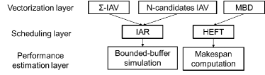
Figure 5. Layered structure of vectorization, scheduling, and performance estimation in the proposed design optimization framework.

6. Experiments using Synthetic Graphs

In this section, we demonstrate the effectiveness of the models and methods developed in Section 5 through experiments that study throughput gain and running time. We compare our methods with the approach of applying graph-level vectorization (GLV) followed by task-graph scheduling.

We use Heterogeneous Earliest Finish Time (HEFT) as the task-graph scheduling method in this comparison. HEFT is a commonly used task-graph scheduling method for HCGPs (e.g., see (Augonnet et al., 2011)). The integration of HEFT with GLV can be viewed as a natural way to integrate SDF vectorization and scheduling using conventional techniques. We refer to the combination of GLV and HEFT as the GLV-HEFT baseline or simply as GLV-HEFT. As implied by this terminology, GLV-HEFT is employed in this experimental study as a baseline for evaluating our proposed methods. The GLV-HEFT baseline applies both GPU acceleration and CPU-GPU multi-processor scheduling. We demonstrate in this section that the ALV and IAR scheduling methods developed in this paper provide significant throughput gain over this baseline approach under given memory constraints.

6.1. Experimental Setup

We have developed an integrated software synthesis framework called DIF-GPU to provide a streamlined workflow that combines actor-level / graph-level vectorization, multi-rate / single-rate SDF scheduling, code generation, and runtime support on heterogeneous computing platforms with multi-core CPUs and GPUs. For details about the DIF-GPU framework, we refer readers to (Lin et al., 2016).

In the experiments presented in this section, we employ an HCGP consisting of a quad-core Intel i5-6400 CPU and an NVIDIA Geforce GTX750 GPU. Actor implementations that are developed for multi-core CPU and GPU execution are compiled using GCC 4.6.3 and the NVIDIA CUDA compiler (NVCC) 7.0, respectively.

6.2. Synthetic Graph Generation

We use Task Graphs For Free (TGFF) (Dick et al., 1998) to generate large sets of synthetic SDF graphs with varied size and complexity. Key parameter settings that we use in TGFF are as follows: the maximum in-degree and out-degree for graph nodes are both set to 3, and the average and multiplier for the lower bound on the number of graph nodes are both set to 20.

From the graph topologies generated by TGFF, we randomly map each graph vertex to a specific DSP actor type that has both a CPU-targeted and GPU-targeted implementation. We perform this vertex-to-actor mapping for all actors in each randomly-generated graph. A broad set of DSP actor types — including actors for cross-correlation, FIR filtering, FFT computation, and vector algebra — are considered when performing this mapping. The GPU-accelerated implementations of these actors provide speedups from 1X to 20X compared to the corresponding multicore CPU implementations. This use of TGFF in conjunction with randomly generated actor mappings helps us to evaluate the performance of our proposed methods on a large variety of graph topologies.

In our experiments, the source and sink actors are selected from a pool of different implementations of data sources and sinks. Because the input/output interfacing functionality in an embedded HCGP is typically implemented on a CPU, we assume that source and sink actors can only be mapped onto CPU cores.

We profile the actors by measuring the execution times of the actors’ firings on the target platform under a series of vectorization degrees. This profiled data is then used as input to the evaluated vectorization and scheduling techniques. The profiled data is also used to simulate the vectorization-integrated schedules that are derived from the proposed and baseline techniques. This simulation is based on the throughput simulator presented in Section 5.5. We use simulation here to enable efficient, automated comparisons across a large variety of different graph structures. In Section 7, we complement this simulation-based evaluation approach with our experimental evaluation of a case study involving an orthogonal frequency-division multiplexing (OFDM) receiver. The evaluation in Section 7 is performed by synthesizing software using DIF-GPU for the targeted HCGP platform, executing the synthesized software on the target platform, and measuring the resulting execution time performance.

6.3. Vectorization

In this section, we apply the different ALV methods introduced in Section 5 to a large collection of synthetic SDF graphs, and evaluate the performance of the derived schedules by simulating their bounded-buffer execution. Note that the baseline for speedup here is GLV-HEFT, where extensive vectorization has been applied, and both the CPU and GPU are used to schedule dataflow actors. This is a much “higher” baseline than single- / multi-core CPU implementation without vectorization. Therefore, the speedup computed over this baseline is relatively small. The synthetic graphs are generated using TGFF together with randomized vertex-to-actor mappings, as described in Section 6.2. We evaluate the speedup over the GLV-HEFT baseline under different memory constraints.

To compare speedups across SDF graphs that have different sizes (i.e., different numbers of actors and edges) and different multirate properties (as defined by the production and consumption rates on the actor ports), we introduce a concept of relative memory bounds as a normalized representation for memory constraints. Given an algorithm $A$ for performing GLV, the relative memory bound $M(G)$ for an SDF graph $G$ is defined as $M(G)=M_{0}\times\alpha$, where $M_{0}$ is the memory cost of the GLV solution derived by Algorithm $A$ when applied to $G$ with $\mathrm{GVD}=1$, and $\alpha$ is a constant that represents the “tightness/looseness” of the applied memory constraint. We experiment with $\alpha\in\{1.0,1.5,\ldots,4.5,5\}$ to cover a series of memory constraints ranging, respectively, from tight to loose.

Figure 6 shows the average simulated speedup that we measured from a set of randomly generated SDF graphs for different techniques for ALV that were introduced in Section 5. As mentioned previously, these speedups are in comparison to baseline solutions that are derived using the GLV-HEFT baseline technique. These results are for a target platform configuration that consists of 1 CPU core and 1 GPU. Here, “TMSV $\Sigma$-IAV” and “TMSVPB $\Sigma$-IAV” represent the $\Sigma$-IAV algorithm with the TMSV and TMSVPB score functions, respectively. The measured throughput gain ranges from 0.8X to 2.4X, and also exhibits significant variation from one SDF graph to another.

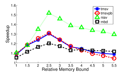
Figure 6. Average speedups measured for four ALV techniques introduced in Section 5: TMSV $\Sigma$-IAV, TMSVPB $\Sigma$-IAV, $N$-candidates IAV, and MBD.

We refer to ALV-IAR as the meta-algorithm that results from applying all four of the proposed ALV techniques, and selecting the best result from among the four derived solutions. In Section 7, we perform further experimental analysis of the ALV-IAR method, which provides a way to leverage complementary benefits of all of the key ALV techniques introduced in Section 5. ALV-IAR is useful, in particular, for design scenarios that can tolerate the relatively large optimization time that is required by $N$-candidates IAV, which dominates the time required by ALV-IAR. ALV-IAR demonstrates average and maximum speedup values of 1.36X and 2.9X on the benchmark set.

We see that $N$-candidates IAV provides the largest average speedup by a significant margin, and this algorithm also provides the largest maximum speedup. We anticipate that this is because $N$-candidates IAV uses more vectorization candidate solutions throughout the search process. The other three ALV techniques achieve similar average and maximum throughput gain.

We have also observed that the average speedup of ALV methods increases until $M(G)=2.5$ and then gradually drops off. When $M(G)$ is close to 1, there is little room for vectorization, so ALV and GLV achieve similar throughput, and the average speedup is close to 1. As $M(G)$ increases to 2.5, more flexibility is provided for ALV to vectorize for better performance than GLV. When $M(G)$ increases beyond 2.5, the memory is sufficient to allow relatively large vectorizations for all actors, so the throughput gain from enabling further vectorization is worn off.

Although the MBD method and the two $\Sigma$-IAV methods achieve smaller average speedup compared to $N$-candidates IAV, they run significantly faster (see Section 6.4), and can be useful in cases where quicker turnaround time is desired from the software synthesis process. In addition, there are cases where they perform better than $N$-candidates IAV.

6.4. Runtime

In this section, we compare the measured running times of the four proposed ALV techniques. We tested the running times of the ALV techniques on the same set $S_{g}$ of randomly generated SDF graphs that we used in the experiments reported on in Section 6.3. The set $S_{g}$ consists of $120$ graphs, where the of number of nodes in a given graph ranges from $3$ to $30$.

Figure 7 shows the measured running times for the four ALV methods with respect to the number of nodes in the input graph. For each of the four ALV methods, there are 120 points plotted in each part of the figure — one point for each graph in $S_{g}$. Thus, Figure 7(a) and Figure 7(b) each depicts a total of $4\times 120=480$ plotted points.

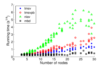
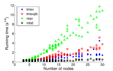
Figure 7. Runtime of ALV methods under different memory constraints: (a) $M=2M_{0}$, and (b) $M=4M_{0}$.

Figure 7 presents running time results associated with two different memory constraints — $M=2M_{0}$ in Figure 7(a), and $M=4M_{0}$ in Figure 7(b) (see the discussion on relative memory bounds in Section 6.3). These two memory constraints are used to represent relatively tight and loose memory budgets, respectively. The vertical axes in Figure 7 correspond to $s^{1/4}$, where $s$ is the measured running time in seconds. Here, we apply an exponent of $(1/4)$ to help improve clarity in depicting the large number of displayed points.

The list of the ALV methods sorted from the fastest to the slowest are: MBD, $\Sigma$-IAV with the TMSV score function, $\Sigma$-IAV with the TMSVPB score function, and NIAV. Note that the TMSVPB score function runs more slowly compared to TMSV due to the computation cost of $\Omega_{\mathit{buf}}(G_{B^{\prime}})$ in the denominator of Equation 4. This cost involves recomputing the buffer requirements for all of the edges in $G$. Table 1 shows the running times of the ALV methods on a specific graph with 22 nodes and 33 edges. This graph is selected randomly to provide further insight into variations in running time among the four ALV methods.

In our experiments, we find that typically MBD finishes within 1 second, while the running times of the two $\Sigma$-IAV methods usually range from several seconds up to a few minutes. We expect that this kind of running time profile is acceptable in many coarse grain dataflow design scenarios in the embedded signal processing domain, where actors typically perform higher level signal processing operations, and therefore the number of nodes in the graphs is limited compared to other types of dataflow graphs that are based on fine-grained actors.

Table 1. The running times (in seconds) of the ALV methods on a specific SDF graph with 22 nodes and 33 edges.

	TMSV $\Sigma$-IAV	TMSVPB $\Sigma$-IAV	NIAV	MBD
$M=2M_{0}$	2.0	8.4	320	0.1
$M=4M_{0}$	13.0	35.9	3500	0.7

The running time of $N$-candidates IAV is generally the longest among all four methods, and grows rapidly with the number of nodes. In our experiments with an SDF graph having 30 nodes, for example, $N$-candidates IAV takes 3 hours to finish its computation. Therefore, $N$-candidates IAV is more suitable in situations when the SDF graph is relatively small, design turnaround time is not critical, or solution quality is of utmost importance.

7. Case Study: OFDM

In this section, we demonstrate the effectiveness of our new ALV-integrated software synthesis framework through a case study involving an orthogonal frequency-division multiplexing (OFDM) receiver (OFDM-RX). The OFDM-RX is an adapted version of the OFDM system described in (Massey et al., 2012). Figure 8 shows an SDF model for the OFDM-RX application. The value above each actor in Figure 8 gives the repetition count of the actor. Table 2 lists the actors in this SDF model and describes their corresponding functions. The system can operate with different parameter values, as shown in Table 3.

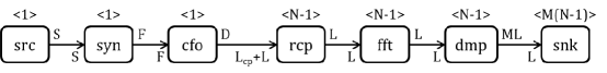
Figure 8. SDF model of OFDM-RX application.

Table 2. Actors in the OFDM-RX application.

Actor	Description
$\mathit{src}$	Read samples of the input signal.
$\mathit{syn}$	Perform time-domain synchronization.
$\mathit{cfo}$	Remove carrier frequency offsets.
$\mathit{rcp}$	Remove cyclic prefix.
$\mathit{fft}$	Perform Fast-Fourier Transform on symbols.
$\mathit{dmp}$	Map OFDM symbols into bit stream.
$\mathit{snk}$	Write bit stream onto the output.

Table 3. Parameters in the OFDM-RX application model, along with the settings or values we use in our experiments.

	Description	Values
$L$	Number of subcarriers per OFDM symbol	[128, 256, 512, 1024]
$N$	Number of OFDM symbols per frame	10
$L_{\mathit{cp}}$	Length of cyclic prefix for each OFDM symbol	$(9/128)L$
$M$	Number of bits per sample	4
$D$	Length of data excluding training symbols	$(N-1)(L+L_{\mathit{cp}})$
$F$	Length of a frame	$N(L+L_{\mathit{cp}})$
$S$	Size of sample stream	$2F$

7.1. System Implementation and Profiling

We have implemented the OFDM-RX actors using the Lightweight Dataflow Environment (LIDE), which provides a programming methodology and associated application programming interfaces (APIs) for implementing dataflow graph actors and edges in a wide variety of platform-oriented languages, such as C, C++, CUDA, and Verilog (Shen et al., 2010; Shen et al., 2011). In our OFDM-RX system, GPU-accelerated implementations are available for all actors other than the $\mathit{src}$ and $\mathit{snk}$ actors. The $\mathit{src}$ and $\mathit{snk}$ actors are not mapped to the GPU in our implementation because of input/output operations that are involved in these actors.

We have profiled the execution times for the OFDM-RX actors on both the CPU and GPU. Figure 9 summarizes the average execution times per SDF graph iteration for the actors. This average time can be expressed as $t_{T}(v)=q(v)t(v)$, where $q$ represents the repetitions vector of the enclosing SDF graph, and $t(v)$ represents the average execution time measured for a single firing of $v$. These execution time estimates are measured on both the CPU and GPU when $L=256$, and the actors are vectorized to process different numbers of data frames per vectorized invocation. Observe from Figure 9 that the distribution of the $t_{T}(v)$ in OFDM-RX are uneven, and that the $\mathit{syn}$ and $\mathit{cfo}$ actors dominate the execution times both on the CPU and GPU. Also, observe that although actor execution times are roughly proportional to the number of frames $N_{F}$, they increase at different rates in relation to $N_{F}$ — for example, $t_{T}(\mathit{cfo})$ on the GPU grows very slowly with increases in $N_{F}$, and $t_{T}(\mathit{syn})$ grows much faster.

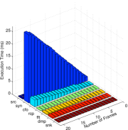
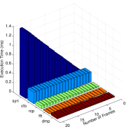
Figure 9. $t_{T}(v)$s on (a) CPU and (b) GPU for OFDM-RX actors that are vectorized to process multiple frames in each firing.

7.2. Software Synthesis with GLV-HEFT

We first measure the performance improvement achieved by GLV-HEFT when integrated in our DIF-GPU software synthesis framework. Here, we measure the system throughput under 11 different configurations without any memory constraints imposed. These measurements are performed on software implementations that are generated automatically using DIF-GPU integrated with GLV-HEFT.

In contrast to the relative throughput metric (see Section 4) that is used as a general performance metric in Section 6, we employ frames per second as the throughput metric more specific to the OFDM-RX application.

We denote the results (throughput values) from these measurements by $\mathit{Th}_{0},\mathit{Th}_{1},\ldots,\mathit{Th}_{10}$. Here, $\mathit{Th}_{0}$, denotes the throughput when the input graph is not vectorized and all actors are mapped onto a single CPU core. On the other hand, for $b\in\{1,2,\ldots,10\}$, $\mathit{Th}_{b}$ represents the throughput obtained when GLV is applied with $\mathrm{GVD}=b$, and HEFT is used to schedule the resulting vectorized graph (GLV-HEFT) (Lin et al., 2016).

Figure 10 shows the speedup in throughput of GLV over the single-CPU implementation, and compares $\mathit{Th}_{0}$ and $\mathit{Th}_{10}$ in more detail for different values of $L$. The maximum measured speedups achieved here are 10.1X, 18.1X, 31.9X, 41.1X for $L=128,256,512,1024$, respectively.

In our experiments, actors in the dataflow model are coarse-grained signal-processing modules. Before vectorization, the actors already encapsulate multiple steps of processing on large signal arrays, and extensively utilize GPU data-parallelism. For example, the unvectorized syn actor in the OFDM receiver application consists of multiple steps of cross-correlation on 20 OFDM symbols. Therefore, saturation at small GVD levels can be expected in Figure 10.

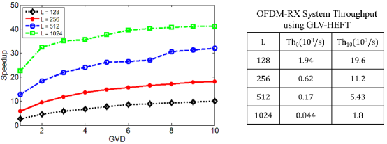
Figure 10. Speedup of the OFDM-RX application over a single CPU implementation for different GVD values and different values of the bandwidth parameter $L$.

7.3. Software Synthesis with ALV-IAR

In this section, we perform measurements and comparisons that involve software implementations that are generated automatically using DIF-GPU integrated with ALV-IAR. The experiments are performed under different memory budgets and different levels of bandwidth $L$ (an application-level parameter). For comparison, we apply DIF-GPU integrated with GLV-HEFT to synthesize software that incorporates vectorized schedules constructed using GLV-HEFT instead of ALV-IAR.

Table 4 shows an example of the vectorization degrees and processor assignments derived for OFDM-RX under a specific memory constraint. This memory constraint is selected to represent one that is neither very tight nor very loose. These vectorized scheduling results are derived by ALV-IAR, and the throughput is measured by executing the resulting software implementation that is synthesized by DIF-GPU. The vectorization and processor assignment (mapping) results are shown in Table 4 as lists of values that correspond to the graph actors in their topological order ($\mathit{src}$, $\mathit{syn}$, …, $\mathit{snk}$). The numbers $0$ and $1$ in the Mapping column represent the CPU-core and GPU, respectively. The results in Table 4 show that ALV-IAR produces a 1.2X speedup compared to the baseline technique for the selected memory constraint.

The memory budgets are set to $M=b\log(L)\times 10^{5}$, where $b=\{1,2,\ldots,10\}$. We compare the throughput levels of implementations generated using the two methods — ALV-IAR and GLV-HEFT — as shown in Figure 11. The results shown in Figure 11 show that using actor-level vectorization and $\Sigma$ scheduling, we are able to obtain system throughput that consistently exceeds that provided by the baseline method under same memory constraint.

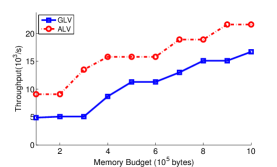
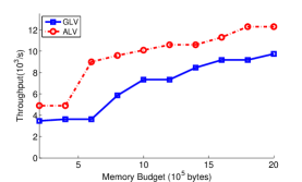
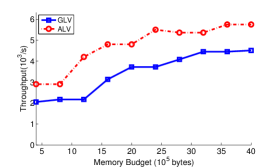
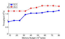
Figure 11. Memory-constrained throughput of OFDM-RX systems with different levels of memory budget $M$ and bandwidth $L$ using ALV-IAR compared to the GLV-HEFT baseline. These experiments are performed on Intel i5-6400 CPU and NVIDIA Geforce GTX750 GPU architectures. (a) $L=128$, (b) $L=256$, (c) $L=512$, (d) $L=1024$.

Table 4. Vectorization degrees and mapping results generated by ALV-IAR and GLV-HEFT under the memory constraint $M=2.8$ Mb, and $L=512$.

Method	Vectorization	Mapping	$\mathit{Th}$($10^{3}/s$)
ALV-IAR	[1,3,12,1,1,1,1]	[0,1,1,0,0,0,0]	3.15
GLV-HEFT	[4,4,4,36,36,36,144]	[0,1,1,1,1,0,0]	2.60

When memory constraints are relatively tight, GLV has difficulty in adequately exploiting data parallelism in the OFDM-RX system. ALV-IAR alleviates this problem by focusing memory resources to vectorize selected, performance-critical actors. Specifically, ALV-IAR successfully identifies $\mathit{syn}$ and $\mathit{cfo}$ as the two actors that benefit the most from vectorized execution on the GPU. Prioritizing the vectorization of these two actors helps to avoid wasting memory on vectorizations that have relatively little or no impact on overall system performance. This is reflected by a large throughput gain when $b\leq 4$. When the memory constraint is relaxed, the gap in the throughput gain between ALV-IAR and GLV is reduced, as data-parallelism in the system can exploited more effectively by GLV under loose memory constraints.

When optimizing the OFDM-RX system, ALV-IAR maps only $\mathit{syn}$ and $\mathit{cfo}$ onto the GPU, and assigns the other actors to the CPU to utilize pipeline parallelism in the system. Under this mapping, firings of $\mathit{syn}$ and $\mathit{cfo}$ from subsequent frames can be executed in parallel with firings of $\mathit{rcp}$, $\mathit{fft}$, $\mathit{dmp}$ and $\mathit{snk}$ from earlier frames.

In these experiments, the maximum measured speedup values of ALV-IAR over GLV-HEFT are 2.66X, 2.45X, 1.94X and 1.71X for $L=128,256,512,1024$, respectively. The maximum speedup values of ALV-IAR compared to a single-core, unvectorized CPU baseline implementation are 11.1X, 19.8X, 33.8X, and 47.6X, for $L=128,256,512,1024$, respectively.

Although the speedup gain of ALV-IAR over GLV-HEFT in this application is significantly higher than the average speedup in Section 6.3, it still falls within the range of the maximum speedup reported in Section 6.3. We expect that this is attributable to the relatively simple, chain-structured topology of the application’s dataflow graph.

The measurements described above are carried out on a CPU-GPU architecture in a desktop computer platform. To complement these experiments using an embedded platform, we investigate the performance of ALV-IAR and GLV-HEFT by performing the same experiments on an NVIDIA Jetson TX1 (TX1). The TX1 is a popular embedded platform that consists of a Quad-core ARM A57 CPU and an NVIDIA Maxwell GPU with 256 CUDA cores. The results are summarized in Figure 12. These results are found to be similar to those obtained using the desktop platform. More specifically, the maximum speedup values of ALV-IAR over GLV-HEFT are 2.4X, 3.5X, 2.4X, 2.5X for $L=128,256,512,1024$, respectively, as measured on the TX1. These results show that ALV-IAR also consistently outperforms GLV-HEFT by a significant margin on the TX1.

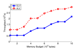
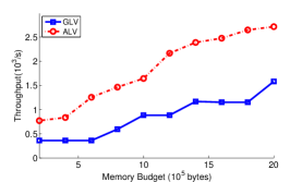
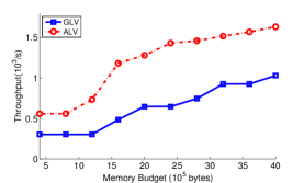
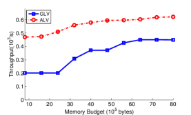
Figure 12. Memory-constrained throughput of OFDM-RX systems with different levels of memory budget $M$ and bandwidth $L$ using ALV-IAR compared to the GLV-HEFT baseline on the NVIDIA Jetson TX1. (a) $L=128$, (b) $L=256$, (c) $L=512$, (d) $L=1024$.

In summary, the throughput improvement obtained by HCGP acceleration using the methods developed in this work facilitates real-time, memory constrained processing of OFDM signals. Such acceleration can benefit a variety of software-defined radio and cognitive radio applications.

8. Conclusion

In this paper, we have investigated memory-constrained, throughput optimization for synchronous dataflow (SDF) graphs on heterogeneous CPU-GPU platforms. We have developed novel methods for Integrated Vectorization and Scheduling (IVS) that provide throughput- and memory-efficient implementations on the targeted class of platforms. We have integrated these IVS methods into the DIF-GPU Framework, which provides capabilities for automated synthesis of GPU software from high-level dataflow graphs specified using the dataflow interchange format (DIF). Our development of novel IVS methods and their integration into DIF-GPU provide a streamlined workflow for automated exploitation of pipeline, data and task level parallelism from SDF graphs. We have demonstrated our IVS methods through extensive experiments involving a large collection of diverse, synthetic SDF graphs, as well as on a practical embedded signal processing case study involving a wireless communications receiver that is based on orthogonal frequency division multiplexing. The results of our experiments demonstrate that our proposed new methods for IVS provide significant improvements in system throughput when mapping SDF graphs onto CPU-GPU platforms. Our proposed methods provide a range of useful trade-offs between analysis time and speedup improvement that designers can select among depending on their specific preferences and constraints.

9. Acknowledgments

This research was supported in part by the Laboratory for Telecommunication Sciences and the National Science Foundation.

References

- (1)
- Augonnet et al. (2011) C. Augonnet, S. Thibault, R. Namyst, and P.-A. Wacrenier. 2011. StarPU: a unified platform for task scheduling on heterogeneous multicore architectures. Journal of Concurrency and Computation: Practice & Experience 23, 2 (February 2011), 187–198.
- Bhattacharyya et al. (2013) S. S. Bhattacharyya, E. Deprettere, R. Leupers, and J. Takala (Eds.). 2013. Handbook of Signal Processing Systems (second ed.). Springer. http://dx.doi.org/10.1007/978-1-4614-6859-2 ISBN: 978-1-4614-6858-5 (Print); 978-1-4614-6859-2 (Online).
- Bhattacharyya et al. (1996) S. S. Bhattacharyya, P. K. Murthy, and E. A. Lee. 1996. Software Synthesis from Dataflow Graphs. Kluwer Academic Publishers.
- Chen and Zhou (2012) Y. Chen and H. Zhou. 2012. Buffer minimization in pipelined SDF scheduling on multi-core platforms. In Proceedings of the Asia South Pacific Design Automation Conference. 127–132.
- Ciccozzi (2013) F. Ciccozzi. 2013. Automatic Synthesis of Heterogeneous CPU-GPU Embedded Applications from a UML Profile. In Proceedings of the International Workshop on Model Based Architecting and Construction of Embedded Systems.
- Desnos et al. (2015) K. Desnos, M. Pelcat, J.-F. Nezan, and Slaheddine Aridhi. 2015. Buffer merging technique for minimizing memory footprints of Synchronous Dataflow specifications. In Proceedings of the International Conference on Acoustics, Speech, and Signal Processing. 1111–1115.
- Dick et al. (1998) R. P. Dick, D. L. Rhodes, and W. Wolf. 1998. TGFF: Task Graphs for Free. In Proceedings of the International Workshop on Hardware/Software Codesign. 97–101.
- Duran et al. (2011) A. Duran, E. Ayguadé, R. M. Badia, J. Labarta, L. Martinell, X. Martorell, and J. Planas. 2011. Ompss: a proposal for programming heterogeneous multi-core architectures. Parallel Processing Letters 21, 2 (2011).
- Ghamarian et al. (2006) A. H. Ghamarian, M. C. W. Geilen, S. Stuijk, T. Basten, A. J. M. Moonen, M. J. G. Bekooij, B. D. Theelen, and M. R. Mousavi. 2006. Throughput analysis of synchronous data flow graphs. In Proceedings of the International Conference on Application of Concurrency to System Design.
- Goli et al. (2012) M. Goli, M. T. Garba, and H. González-Vélez. 2012. Streaming Dynamic Coarse-Grained CPU/GPU Workloads with Heterogeneous Pipelines in FastFlow. In Proceedings of HPCC-ICESS. 445–452.
- Gregg and Hazelwood (2011) C. Gregg and K. Hazelwood. 2011. Where is the data? Why you cannot debate CPU vs. GPU performance without the answer. In Proceedings of the IEEE International Symposium on Performance Analysis of Systems and Software. 134–144.
- Hagiescu et al. (2011) A. Hagiescu, H. P. Huynh, W.-F. Wong, and R. S. M. Goh. 2011. Automated Architecture-Aware Mapping of Streaming Applications Onto GPUs. In Proceedings of the International Symposium on Parallel and Distributed Processing. 467–478.
- Hsu et al. (2011) C. Hsu, J. Pino, and S. S. Bhattacharyya. 2011. Multithreaded Simulation for Synchronous Dataflow Graphs. ACM Transactions on Design Automation of Electronic Systems 16, 3 (June 2011), 25–1–25–23.
- Ko et al. (2008) M. Ko, C. Shen, and S. S. Bhattacharyya. 2008. Memory-constrained Block Processing for DSP Software Optimization. Journal of Signal Processing Systems 50, 2 (February 2008), 163–177.
- Lee and Messerschmitt (1987) E. A. Lee and D. G. Messerschmitt. 1987. Synchronous Dataflow. Proc. IEEE 75, 9 (September 1987), 1235–1245.
- Lin et al. (2016) S. Lin, Y. Liu, W. Plishker, and S. S. Bhattacharyya. 2016. A Design Framework for Mapping Vectorized Synchronous Dataflow Graphs onto CPU–GPU Platforms. In Proceedings of the International Workshop on Software and Compilers for Embedded Systems. Sankt Goar, Germany, 20–29. http://portal.acm.org/dl.cfm
- Lund et al. (2015) W. Lund, S. Kanur, J. Ersfolk, L. Tsiopoulos, J. Lilius, J. Haldin, and U. Falk. 2015. Execution of Dataflow Process Networks on OpenCL Platforms. In Euromicro International Conference on Parallel, Distributed, and Network-Based Processing. 618–625.
- Massey et al. (2012) J. W. Massey, J. Starr, S. Lee, D. Lee, A. Gerstlauer, and R. W. Heath. 2012. Implementation of a real-time wireless interference alignment network. In Proceedings of the IEEE Asilomar Conference on Signals, Systems, and Computers. 104–108.
- Park and Dally (2010) J. Park and W. J. Dally. 2010. Buffer-space efficient and deadlock-free scheduling of stream applications on multi-core architectures. (2010).
- Ritz et al. (1993) S. Ritz, M. Pankert, and H. Meyr. 1993. Optimum Vectorization of Scalable Synchronous Dataflow Graphs. In Proceedings of the International Conference on Application Specific Array Processors.
- Schor et al. (2013) L. Schor, A. Tretter, T. Scherer, and L. Thiele. 2013. Exploiting the parallelism of heterogeneous systems using dataflow graphs on top of OpenCL. In Proceedings of the IEEE Workshop on Embedded Systems for Real-Time Multimedia. 41–50.
- Shen et al. (2010) C. Shen, W. Plishker, H. Wu, and S. S. Bhattacharyya. 2010. A Lightweight Dataflow Approach for Design and Implementation of SDR Systems. In Proceedings of the Wireless Innovation Conference and Product Exposition. 640–645.
- Shen et al. (2011) C. Shen, L. Wang, I. Cho, S. Kim, S. Won, W. Plishker, and S. S. Bhattacharyya. 2011. The DSPCAD Lightweight Dataflow Environment: Introduction to LIDE Version 0.1. Technical Report UMIACS-TR-2011-17. Institute for Advanced Computer Studies, University of Maryland at College Park. http://hdl.handle.net/1903/12147.
- Sriram and Bhattacharyya (2009) S. Sriram and S. S. Bhattacharyya. 2009. Embedded Multiprocessors: Scheduling and Synchronization (second ed.). CRC Press. ISBN:1420048015.
- Stuijk et al. (2006) S. Stuijk, M. Geilen, and T. Basten. 2006. Exploring Tradeoffs in Buffer Requirements and Throughput Constraints for Synchronous Dataflow Graphs. In Proceedings of the Design Automation Conference.
- Topcuoglu et al. (2002) H. Topcuoglu, S. Hariri, and M.-Y. Wu. 2002. Performance-effective and low-complexity task scheduling for heterogeneous computing. IEEE Transactions on Parallel and Distributed Systems 13, 3 (2002), 260–274.
- Tripakis et al. (2013) S. Tripakis, D. Bui, M. Geilen, B. Rodiers, and E. A. Lee. 2013. Compositionality in synchronous data flow: Modular code generation from hierarchical SDF graphs. ACM Transactions on Embedded Computing Systems 12, 3 (2013).
- Udupa et al. (2009) A. Udupa, R. Govindarajan, and M. J. Thazhuthaveetil. 2009. Software Pipelined Execution of Stream Programs on GPUs. In Proceedings of the International Symposium on Code Generation and Optimization. 200–209.
- Zaki et al. (2013) G. Zaki, W. Plishker, S. S. Bhattacharyya, C. Clancy, and J. Kuykendall. 2013. Integration of Dataflow-based Heterogeneous Multiprocessor Scheduling Techniques in GNU Radio. Journal of Signal Processing Systems 70, 2 (February 2013), 177–191.