Supplementary Material for ABC-GAN paper

Appendix A Small-scale synthetic experiments

A.1 Univariate normal distribution

We generate $N=1000$ observations from the univariate normal distribution with mean $\mu_{0}=3$ and variance $\sigma^{2}_{0}=1$. We use the following priors:

$$\mu\sim Unif(0,5),\qquad\sigma^{2}\sim Unif(1,5),$$ (1)

and perform parameter estimation ($\hat{\mu}$ and $\hat{\sigma}^{2})$ using rejection sampling, BOLFI and ABC-GAN. Table 1 shows the timing (in seconds) and accuracy results for the three approaches. We note that BOLFI is a complex method and is unsuited for this case since generation of univariate normal samples is computationally very cheap. Nonetheless, we observe that ABC-GAN converges in reasonable time and gives comparable results to others approaches.

Method	$\hat{\mu}$	$\hat{\sigma}^{2}$	$t$ (in seconds)
ABC	2.92	1.17	0.147
BOLFI	2.68	1.13	2700
GAN	3.023	1.04	37.12

Table 1: We compare the results with naive ABC (using rejection sampling for $10000$ samples) and BOLFI algorithm (Rejection sampling and ABC were implemented using ELFI (kangasraasio2016elfi)).

For low-dimensional problems with i.i.d. samples where simulation cost is cheap, classic ABC methods are best in terms of ease of implementation and wall-clock time.

A.2 Mixture of normals

We consider a mixture of two normal distributions, first studied in sisson2007sequential, with the observations generated from:

$$P_{\theta}(\theta)\sim\frac{1}{2}{\cal N}(0,\frac{1}{100})+\frac{1}{2}{\cal N}(0,1)$$ (2)

Here the second term implies large regions of low probability in comparison to the first term. Both classic rejection sampling and Monte Carlo ABC suffer from low acceptance rate and consequently, longer simulation runs (respectively, $400806$ and $75895$ steps) when generating samples from the low probability tail region.

In contrast, we run ABC-GAN for $5000$ iterations with a mini-batch size of $10$ and sequence length $10$, using a learning rate $10^{-3}$.

Figure 1 shows the generated posterior samples and we see that the posterior samples capture the low probability component of the probability density function. We also run BOLFI (kangasraasio2016elfi) in order to compare its result to ABC-GAN.

Table 2 presents the timing and accuracy for the different methods. The accuracy is specified in terms of Kullback-Liebler divergence (cover2012elements) between the true pdf and the empirical pdf estimated using posterior samples in the range [-10, 10]. We note that the KL-divergence of BOLFI w.r.t. true pdf is lower compared to the KL divergence of ABC-GAN w.r.t. true pdf. However, this does not translate to capturing the low-probability space as shown in Figure 1 (b) where BOLFI does not have samples in the low-dimensional space.

We note that BOLFI fails to adequately capture the low-probability space (due to the second component) of the problem. This is reflected in Table 2. Additionally, the BOLFI implementation in ELFI is considerably slower than ABC-GAN and this scenario is exacerbated as more number of observations are provided or more simulation samples are generated due to the use of Gaussian Processes.

(a)	(b)

Figure 1: $(a)$ Posterior samples for ABC-GAN (shown in green) for one run in the mixture of normals experiment (Section A.2) with $5000$ iterations with a mini-batch size of $10$ and sequence length $10$, using a learning rate $10^{-3}$. The probability density function for the mixture normal and the low-variability component are shown in red and blue respectively. $(b)$ Histogram of posterior samples for first run of BOLFI. Total number of samples is $5000$. We note that the low-probability space is not captured by BOLFI compared to ABC-GAN.

Method	$n_{s}$	$D_{KL}(p\|q)$	$t$
rej. sampl.†	5000	$0.567\pm 0.012$	0.22
ABC-GAN	5000	$0.539\pm 0.196$	14.70
BOLFI†	1000	$0.627\pm 0.417$	126.71
BOLFI†	5000	$0.445\pm 0.027$	426.03

Table 2: Timing and accuracy information for the mixture of normals example averaged over $10$ independent runs. The the number of samples generated by the simulator ($n_{s}$) are shown. The Kullback-Liebler divergence ($D_{KL}(p\|q)$) between the true pdf $(p)$ and the empirical pdf estimated using accepted samples ($q$) and the time taken (for the first run) in seconds ($t$) are shown. ^†ELFI returns only negative samples so we add $-x$ to the samples for each original sample $x$ before computing the KL divergence.

A.3 Inference in multi-variate normal

We consider multivariate normal model ${\bf X}\in\Re^{16}$ with true mean $\bf 1$ and prior on mean $x_{i}\sim{\tt Uniform}(0,10)$. We use two layer feed-forward neural networks as our generator and approximator units. A learning rate of $10^{-3}$ and a hidden layer of size $16$ is used in the approximator and generator units. MMD Loss is used as a surrogate for the discriminator as well as for comparing the output of the approximator unit with the simulator.

Figure 2: Inferred parameters for one run of ABC-GAN for the multi-variate normal model (Section A.3). We see that the inferred parameters are close to the true mean $\bf 1$.

Figure 3: The L1-loss between the inferred and the true mean in the multi-variate normal example (Section A.3) as the algorithm progresses.

Figures 2 and 3 show the inferred parameters and the L1-loss between the inferred mean and the true mean as the algorithm progresses. We note that the inferred parameters are close to the true mean $\bf 1$. The total time taken is 46.38 seconds.

Appendix B ABC-GAN specification for Ricker’s model

This section presents the complete model specification of our GAN architecture for the Ricker’s model. We describe each of the individual sub-networks below.

For sake of completeness, we recall the prior distribution on the parameters $\theta=(\log r,\sigma,\phi)$ given by:

$$\begin{array}[]{r}\log r\sim\tt{Uniform}(0,5),\\ \sigma\sim\tt{Uniform}(0,1),\\ \phi\sim\tt{Uniform}(0,15).\end{array}$$

In the remainder of this section, the notation $(d=10)$ indicates the layer has $10$-dimensional output.

Generator

The generator $G_{u}(\cdot)$ takes as input the samples from the prior distribution on $\theta=(\log r,\sigma,\phi)$. The generator has the following equations:

$$x_{G,1} ={\tt ReLu}(w_{g,1}^{\top}\theta+b_{g,1}) (d=20)$$

$$x_{G,2} =w_{u,2}^{\top}x_{g,2}+b_{g,2} (d=3)$$

$$x_{G,3} =5\times{\tt Sigmoid}(x_{G,2}[:,1]) (d=1) (\hat{\log r})$$

$$x_{G,4} ={\tt Sigmoid}(x_{G,2}[:,2]) (d=1) (\hat{\sigma})$$

$$x_{G,5} =15\times{\tt Sigmoid}(x_{G,2}[:,3]) (d=1) (\hat{\phi})$$

$$x_{G} =[x_{G,3},\,x_{G,4},\,x_{G,5}] (d=3) (\hat{\theta}_{post})$$

The complete set of weights are given by $W_{G}=\{w_{g,i},b_{g,i}\forall i\in 1,2\}$ which are initialized using samples from the normal distribution ${\cal N}(0,1)$.

Approximator

The approximator unit consists of a feed-forward layer which takes as input the posterior parameters $x_{G}$ from the generator and outputs approximate statistics given as:

$$x_{A} =w_{a,1}^{\top}x_{G}+b_{a,1} (d=3)$$

where the weights $W_{A}=\{w_{a,1},b_{a,1}\}$ are initialized from the normal distribution ${\cal N}(0,1)$.

Summarizer

The summarizer unit consists of LSTM cell followed by a dense layer which projects the sequence to the summary representation. We recall that the standard LSTM unit is defined as:

$$f_{t} =\sigma(W_{f}\cdot[h_{t-1},x_{t}]+b_{f})$$ (forget gate)

$$i_{t} =\sigma(W_{i}\cdot[h_{t-1},x_{t}]+b_{i})$$ (input gate)

$$\tilde{C}_{t} =tanh(W_{c}\cdot[h_{t-1},x_{t}]+b_{C})$$

$$C_{t} =f_{t}*C_{t-1}+i_{t}*\tilde{C}_{t}$$ (cell state)

$$o_{t} =\sigma(W_{o}\cdot[h_{t-1},x_{t}]+b_{o})$$ (output)

$$h_{t} =o_{t}*tanh(C_{t})$$

where $W_{LSTM}=\{W_{f},W_{i},W_{C},W_{o},b_{f},b_{i},b_{C},b_{o}\}$ are the weights for a single unit. We use the notation ${\tt LSTM}_{k}$ to denote $k$ LSTM units connected serially.

Given input sequence $seq$ obtained from the simulator or from observed data, the summarizer output is given by:

$$x_{S,1} ={\tt LSTM}_{k}(seq) (d=k=10)$$

$$x_{S} =w_{s,1}^{\top}x_{S,1}+b_{s,1} (d=10)$$

where the weights are given by $W_{S}=\{w_{S,1},b_{S,1}\}\cup w_{LSTM}$. The weights are initialized to normal distribution and the initial cell state is set to zero tuple of appropriate size.

Optimization

The connections are described as follows:

$$x_{G} ={\cal G}(\theta;W_{G})$$

$$x_{A} ={\cal A}(x_{G};W_{A})$$

$${\tt seq}_{S} ={\tt simulator}(x_{G},\epsilon)$$

$$x_{S} ={\cal S}({\tt seq}_{S};W_{S})$$

$$x_{O} ={\cal S}({\tt seq}_{O};W_{S})$$

where ${\tt seq}_{O}$ denotes the observed data, $x_{O}$ is its summary representation obtained using the summarizer, and $\epsilon$ denotes normal noise for input to the simulator alongwith the posterior parameter $X_{G}$.

We use maximum mean discrepancy (MMD) loss (dziugaite2015training) to train the network. Given reproducing kernel Hilbert space (RKHS) ${\cal H}$ with associated kernel $k(\cdot,\cdot)$ and data $X,X^{\prime},X_{1},\ldots,X_{N}$ and $Y,Y^{\prime},Y_{1},\ldots,Y_{M}$ from distributions $p$ and $q$ respectively, the maximum mean discrepancy loss is given by:

$$MMD^{2}[{\cal H},p,q] =E[k(X,X^{\prime})-2k(X,Y)+k(Y,Y^{\prime})].$$

We use the Gaussian kernel and define the following loss functions:

$${\cal L}_{G}=MMD(x_{A},x_{O})$$

$${\cal L}_{R}=MMD(x_{A},x_{S})$$

Let $W_{R}=(W_{S},W_{A})$ denote the combined weights for the summarizer and the approximator units. The update equations for the network are then given by the following alternating optimizations:

$$W_{R}^{(i+1)} \leftarrow W_{R}^{(i)}+\alpha\cdot{\tt RMSProp}(\nabla_{W_{A},W_{S}}{\cal L}_{R})$$

$$W_{G}^{(i+1)} \leftarrow W_{G}^{(i)}+\alpha\cdot{\tt RMSProp}(\nabla_{W_{G}}{\cal L}_{R})$$

where $\alpha$ is the learning rate for the RMSProp algorithm.

Appendix C Hand-engineered features for the DCC model

numminen2013estimating defined four summary statistics per day care center in order to characterize the simulated and observed data and perform ABC-based inference of the parameters ${\Theta}=(\Lambda,\beta,\theta)$:

• The strain diversity in the day care centers,

• The number of different strains circulating,

• The fraction of the infected children,

• The fraction of children infected with multiple strains.

gutmann2017likelihood classified the simulated data as being fake (not having the same distribution as the observed data) or based on the following features:

1. $L2$-norm of the singular values and the rank of the original matrix (2 features),

2. The authors computed the fraction of ones in the set of rows and columns of the matrix. Then, the average and the variability of this fraction was taken across the whole set of rows and columns. Since the average is the same for the set of rows and columns, this yields 3 features.

3. The same features as $(2)$ above for a randomly chosen sub-matrix having $10\%$ of the elements of the original matrix (2 features).

By choosing $1000$ random subsets, the authors converted the set of $29$ matrices to a set of $1000$ seven-dimensional features. This feature set was used to perform classification using LDA. They also did the classification without the randomly chosen subsets mapping each simulated dataset to a five-dimensional feature vector.

Appendix D ABC-GAN specification for the DCC model

This section presents the complete description for our architecture doing likelihood free inference in the Daycare center example. We describe each of the sub-networks below.

Generator

The generator ${\cal G}(\cdot)$ takes as input the samples from the prior distribution on $\Theta=(\Lambda,\beta,\theta)$. It is specified as follows:

$$x_{G,1} =w_{g,1}^{\top}\Theta+b_{g,1} (d=3)$$

$$\hat{\Lambda} =12\cdot\sigma(x_{G,1}[:,0]) (d=1)$$

$$\hat{\beta} =2\cdot\sigma(x_{G,1}[:,1]) (d=1)$$

$$\hat{\theta} =\sigma(x_{G,1}[:,2]) (d=1)$$

$$x_{G} =[\hat{\Lambda}\;\hat{\beta}\;\hat{\theta}]$$

The set of variables are given by $W_{G}=[w_{g,1},b_{g,1}]$ which are initialized using normal distribution.

Approximator

The approximator unit has a feed-forward network given by:

$$x_{A} =w_{a,1}^{\top}x_{G}+b_{a,1}$$

where $W_{A}=[w_{a,1},b_{a,1}]$ are the weights which are initialized using the normal distribution.

Appendix E Supplemental Figures

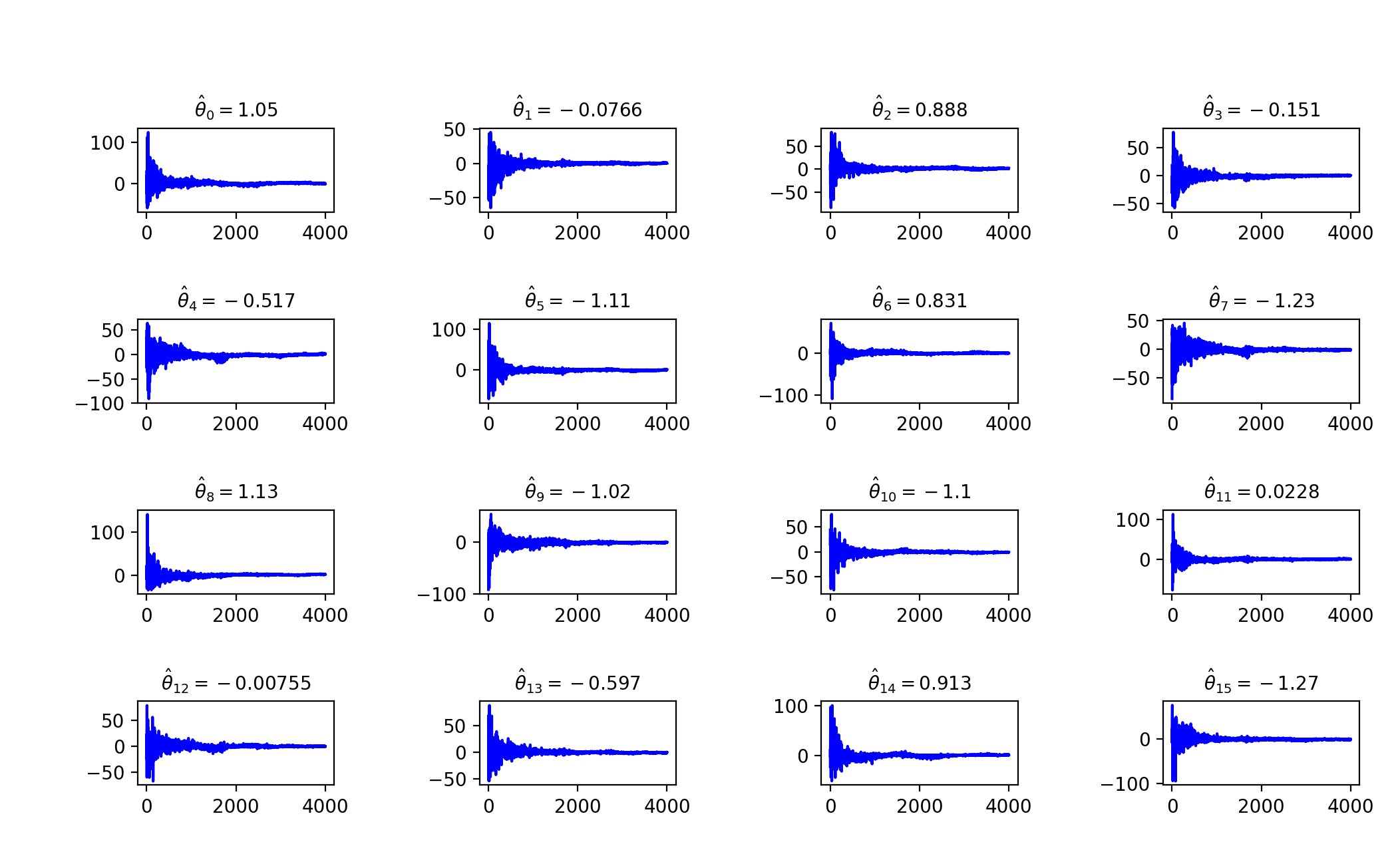
Figure 4: Inferred parameter values (true parameter is $\bf 0$) with prior $\theta_{i}\sim{\tt Uniform}(-100,100)$ and two layer feed-forward networks used for the generator and approximator in the ABC-GAN structure.

• Figure 4 shows the inferred parameter values in Section 4.1.3 of the main manuscript. The true parameter is $\bf 0$ with prior $\theta_{i}\sim{\tt Uniform}(-100,100)$ and two layer feed-forward networks used for the generator and approximator in the ABC-GAN structure.