CERN-TH-2017-247

TTP17-047

Three-loop mixed QCD-electroweak corrections to Higgs boson gluon fusion

Marco Bonetti^a, , Kirill Melnikov^a, and Lorenzo Tancredi^b,
a Institute for Theoretical Particle Physics, KIT, 76128 Karlsruhe, Germany

^b CERN Theory Division, CH-1211, Geneva 23, Switzerland

We compute the contribution of three-loop mixed QCD-electroweak corrections ($\alpha_{S}^{2}\alpha^{2}$) to the $gg\to H$ scattering amplitude. We employ the method of differential equations to compute the relevant integrals and express them in terms of Goncharov polylogarithms.

Key words: Higgs gluon fusion, electroweak corrections, 3-loop computations.

1 Introduction

It is an open question if the scalar boson discovered by ATLAS and CMS collaborations in 2012 is indeed the Higgs boson of the Standard Model. To answer this question, Higgs boson production cross sections and decay rates are measured experimentally and compared to theoretical predictions. Thanks to the renormalizability of the Standard Model, properties of the Higgs boson, including its quantum numbers and its couplings to gauge bosons and matter particles, are completely fixed. As a result, it is possible, at least in principle, to describe production and decay of the Higgs boson in the Standard Model with unlimited precision.

On the other hand, if the Standard Model is not a complete theory, New Physics at scale $\Lambda$ that couples to the Higgs boson is expected to modify its couplings to matter and gauge particles by an amount $\delta g/g\sim{\cal O}(v^{2}/\Lambda^{2})$ where $v=246\leavevmode\nobreak\ {\rm GeV}$ is the scale of electroweak symmetry breaking. Taking $\Lambda=1\leavevmode\nobreak\ {\rm TeV}$, we find a typical modification in Higgs couplings of about $5\%$, which sets a precision goal for both experimental measurements and theoretical computations.

The major Higgs-boson production channel at the LHC is gluon fusion $gg\to H$; it contributes more than $90\%$ to the total Higgs production cross section at $13\,\mathrm{TeV}$. As discussed in Refs. [1, 2], almost $5\%$ of the gluon fusion cross section comes from mixed QCD-electroweak (QCD-EW) contributions where the Higgs boson couples to electroweak gauge bosons that, later, convert to gluons through a quark loop. The remaining $95\%$ of the $gg\to H$ cross section is generated by pure QCD interactions.

The importance of the $gg\to H$ channel for the investigation of the Higgs boson properties motivated its extensive studies in the past. Since the Higgs boson is light and the top quarks are relatively heavy, it is possible to integrate them out and work with an effective Lagrangian where the $ggH$ coupling is point-like. The $gg\to H$ production cross section in the $m_{t}\to\infty$ approximation is known through N³LO in QCD while other, smaller contributions, are known less precisely.

At present, the theoretical uncertainty in $gg\to H$ cross section originates from (see [1, 2]) the ${\cal O}(2\%)$ residual scale uncertainty in pure QCD contributions, the ${\cal O}(1\%)$ uncertainty caused by unknown mass effects of $b$ and $c$ quarks in higher orders of QCD perturbation theory, and the ${\cal O}(1\%)$ uncertainty in QCD-EW contributions. The latter uncertainty is particularly peculiar since computation of QCD corrections to mixed QCD-EW contributions exists [3]. However, although the leading order QCD-EW $\mathcal{O}(\alpha_{S}^{\leavevmode\nobreak\ }\alpha^{2})$ contribution is known for arbitrary values of the Higgs and electroweak gauge boson masses [4, 5, 6, 7], the next-to-leading order (NLO) QCD corrections to it have only been computed in the unphysical limit $m_{H}\ll m_{W,Z}$ [3]. It turns out [3] that in this approximation the QCD corrections to mixed QCD-EW contributions are large and, in fact, similar to NLO corrections to leading QCD contributions. Nevertheless, the magnitude of QCD corrections and the approximate nature of the calculation of Ref. [3] are major reasons for assigning a large uncertainty to the QCD-EW contribution to $gg\to H$ in Ref. [1]. To remove this theoretical uncertainty, the NLO QCD corrections to QCD-EW contribution to $gg\to H$ should be re-computed for physical values of $m_{H},m_{W}$ and $m_{Z}$.

The goal of this paper is to present one of the ingredients of such a computation – the virtual QCD corrections to mixed QCD-EW contribution to $gg\to H$ amplitude. The NLO QCD-EW corrections are given by three-loop $\mathcal{O}(\alpha_{S}^{2}\alpha^{2})$ diagrams where gluons couple to electroweak gauge bosons through quark loops, and electroweak gauge bosons fuse into Higgs boson. In principle, all quark flavors contribute to mixed QCD-EW corrections but, since the Higgs boson is light, the contribution of top quark loops is small [3]. For this reason we focus on the contribution of massless quarks in what follows.

To compute the three-loop mixed QCD-EW contribution to the $gg\to H$ amplitude, we use the method of differential equations [8, 9, 10] to calculate the relevant master integrals (MIs). We employ the concept of canonical basis introduced in Ref.[11], and express the MIs in terms of Goncharov’s multiple polylogarithms (GPLs) [12, 13, 14], up to weight 6. We use the mathematical limit of small Higgs mass $m_{H}\ll m_{W,Z}$ to determine the boundary values for the solutions of the differential equations. Our final three-loop result for QCD-EW contributions to $gg\to H$ amplitude is expressed in terms of GPLs up to weight five.

The paper is organized as follows. We introduce the gluon fusion amplitude $gg\to H$ and discuss the QCD-EW contributions in Section 2. In Section 3 we describe the classes of integrals that contribute to the QCD-EW amplitude. In Section 4 we discuss differential equations for MIs and their simplification to a canonical form. We introduce the large-mass expansion in Section 5 and explain how we use it to provide boundary conditions for the solutions of the differential equations. The final result for the $gg\to H$ amplitude is given in Section 6. We conclude in Section 7. Additional information about integral topologies and MIs can be found, respectively, in Appendices A and B. We provide the analytic results for leading and next-to-leading order QCD-EW contributions to $gg\to H$ amplitude in the ancillary file.

Additional material that includes the expressions for MIs, the basis of canonical functions, the matrix of coefficients of the differential equations and the integration constants is available at https://www.ttp.kit.edu/_media/progdata/2017/ttp17-047/anc.tar.gz.

2 QCD-EW contribution to $gg\to H$ amplitude

We show the mixed QCD-electroweak corrections to the $gg\to H$ amplitude in Fig. 1. They appear for the first time at two loops. The two gluons annihilate to electroweak vector bosons through a quark loop. The vector bosons fuse into a Higgs boson in a second step. These leading order QCD-electroweak contributions are well-known [4, 5, 6, 7]. Our goal in this paper is to compute the QCD corrections to the leading order QCD-EW contribution to $gg\to H$ amplitude.

Both $W$ and $Z$ bosons appear in diagrams that contribute to the QCD-EW amplitude. In the case of $W$-bosons, we account for quarks of the first two generations; when considering $Z$-bosons, we include, in addition, bottom quarks. We treat all quarks as massless. To write an expression for the $gg\to H$ amplitude we assume that the two incoming gluons $g_{1}$ and $g_{2}$ carry on-shell momenta $p_{1,2}$, color indices $c_{1,2}$ and polarization labels $\lambda_{1,2}$. The momentum of the outgoing Higgs boson is taken to be $p_{3}=-p_{1}-p_{2}$, with $p_{3}^{2}=m_{H}^{2}=s$.

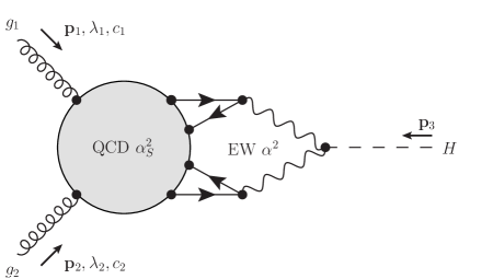
Figure 1: Mixed QCD-EW corrections to Higgs boson production in gluon fusion. The powers of the couplings refer to NLO contributions.

QCD gauge invariance ensures that the $gg\to H$ amplitude depends on a single form factor

$$\mathcal{M}^{c_{1}c_{2}}_{\lambda_{1}\lambda_{2}}=\mathcal{F}\left(s,m_{W}^{2},m_{Z}^{2}\right)\;\delta^{c_{1}c_{2}}\;\varepsilon_{\lambda_{1}}(\mathbf{p}_{1})\cdot\varepsilon_{\lambda_{2}}(\mathbf{p}_{2}),$$ (2.1)

where $\varepsilon_{\lambda_{1,2}}$ are gluon polarization vectors that satisfy the transversality conditions $\varepsilon_{\lambda_{i}}\cdot p_{1}=\varepsilon_{\lambda_{i}}\cdot p_{2}=0$, for $i=1,2$. It is convenient to construct a projection operator that can be applied to individual Feynman diagrams to extract their contributions to the form factor $\mathcal{F}$. The projection operator reads

$$\mathbb{P}_{c_{1}c_{2}}^{\lambda_{1}\lambda_{2}}=\frac{\varepsilon^{*\lambda_{1}}(\mathbf{p}_{1})\cdot\varepsilon^{*\lambda_{2}}(\mathbf{p}_{2})}{d-2}\frac{\delta_{c_{1}c_{2}}}{N_{c}^{2}-1},$$ (2.2)

where $d=4-2\varepsilon$ is the space-time dimensionality. Using the standard expression for the sum over polarizations for each of the two gluons, consistent with the transversality conditions

$$\sum\limits_{\lambda_{i}=\pm}\varepsilon^{\mu}_{\lambda_{i}}(\mathbf{p}_{i})\varepsilon^{*\lambda_{i},\nu}(\mathbf{p}_{i})=-g^{\mu\nu}+\frac{p_{1}^{\mu}p_{2}^{\nu}+p_{1}^{\nu}p_{2}^{\mu}}{p_{1}\cdot p_{2}},$$ (2.3)

it is easy to show that the following equation holds

$$\mathcal{F}\left(s,m_{W}^{2},m_{Z}^{2}\right)=\sum_{\lambda_{1},\lambda_{2},c_{1},c_{2}}\mathbb{P}_{c_{1},c_{2}}^{\lambda_{1}\lambda_{2}}\mathcal{M}_{\lambda_{1}\lambda_{2}}^{c_{1},c_{2}}.$$ (2.4)

We can further simplify this equation if we write the amplitude as

$$\mathcal{M}^{c_{1}c_{2}}_{\lambda_{1}\lambda_{2}}={\cal A}^{c_{1}c_{2}}_{\mu\nu}\varepsilon^{\mu}_{\lambda_{1}}(\mathbf{p}_{1})\varepsilon^{\nu}_{\lambda_{2}}(\mathbf{p}_{2}),$$ (2.5)

apply the projection operator and sum over helicity labels of the two gluons, to obtain

$$\mathcal{F}\left(s,m_{W}^{2},m_{Z}^{2}\right)=\frac{{\cal A}^{c_{1}c_{2}}_{\mu\nu}\delta_{c_{1}c_{2}}}{(N_{c}^{2}-1)(d-2)}\left(-g^{\mu\nu}+\frac{p_{1}^{\mu}p_{2}^{\nu}+p_{1}^{\nu}p_{2}^{\mu}}{p_{1}\cdot p_{2}}\right).$$ (2.6)

This formula can be used to extract the contribution of individual diagrams to the gauge-invariant form factor $\mathcal{F}$.

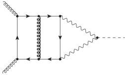
(a)

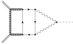
(b)

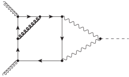
(c)

Figure 2: Examples of QCD corrections to the LO QCD-EW Higgs gluon fusion.

Examples of three loop diagrams that contribute to the NLO QCD corrections to the mixed QCD-electroweak $gg\to H$ amplitude are shown in Fig. 2. The majority of the diagrams contributes both to $Z$ and $W$ channels with a few exceptions that contribute only in the $Z$ channel; some examples are shown in Fig. 3. However, all diagrams that distinguish $Z$ and $W$ contributions vanish either because of color algebra (Fig. 3a), or Furry’s theorem (vector current contribution in case of Fig. 3b) or the fact that we consider complete generations of massless quarks (Fig. 3b, axial current). We note that in the latter case, because of the axial anomaly, the contribution of the $b$-quark is not well defined without the top quark; in this paper we ignore this issue and completely discard all contributions that lead to diagrams of the type (Fig. 3b) but we include the $b$-quark in all other three-loop QCD-EW diagrams that we consider in this paper. After these simplifications, there remain 47 three-loop non-vanishing diagrams for both $W$-bosons and the $Z$-bosons. All the relevant contributions can be obtained by considering diagrams where a massive vector boson interacts with the quark loop through a vector current.

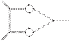
(a)

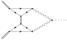
(b)

Figure 3: Typical diagrams that may provide $Z$- but not $W$-boson contributions to mixed QCD-EW corrections.

3 Topologies and master integrals

It is straightforward to compute contributions of individual diagrams to the invariant form factor $\mathcal{F}$ using Eq. (2.6). Upon doing so, we find that the form factor $\mathcal{F}$ is given by a linear combination of Feynman integrals that we write as follows

$$\int\frac{\mathrm{d}^{d}k_{1}\,\mathrm{d}^{d}k_{2}\,\mathrm{d}^{d}k_{3}}{\left[{\mathrm{i}\mathrm{\pi}^{d/2}\Gamma(1+\varepsilon)}\right]^{3}}\,\prod_{j=1}^{J}\frac{1}{[j]^{a_{j}}}.$$ (3.1)

The $[j]$s denote inverse Feynman propagators that we specify in Appendix A. Since $W$ and $Z$ bosons never appear in the same Feynman diagram, we use a generic notation $M$ for the mass of the vector bosons when we discuss Feynman diagrams and integrals. All Feynman integrals are analytic functions in the variables $s=(p_{1}+p_{2})^{2}$ and $M^{2}$ . Discontinuities common to all parent topologies occur at $s\geq 0$ (on-shell massless intermediate states), $s\geq M^{2}$ (production of an on-shell vector boson plus two massless quarks), and $s\geq 4M^{2}$ (production of an on-shell pair of vector bosons).

To compute the different Feynman integrals contributing to the form factor, we identify eleven different topologies; these topologies can be written using three different sets of the inverse Feynman propagators. The topologies are described in Appendix A. We use the program Reduze2 [15] to express all Feynman integrals that contribute to the invariant form factor $\mathcal{F}$ through 95 master integrals (MIs). The full list of MIs can be found in Appendix B.

4 Differential equations

4.1 General considerations

To calculate the MIs, we employ the differential equations method. The MIs depend on two dimensionfull variables $s$ and $M^{2}$ and it is convenient to trade them for one dimensionfull and one dimensionless variable. We take $s$ to be the dimensionfull variable, extract the mass dimensions of the MIs and write

$$I_{n}(\varepsilon,s,y)=(-s)^{-a_{n}-3\varepsilon}J_{n}(\varepsilon,y).$$ (4.1)

The dimensionless variable $y$ reads

$$y=\frac{\sqrt{1-4{M^{2}}/{s}}-1}{\sqrt{1-4{M^{2}}/{s}}+1}.$$ (4.2)

Values of the variable $y$ for different relations between $M^{2}$ an $s$ are shown in Table 1, together with prescriptions for analytic continuation.

Variable	Prescription	Euclidean region	Minkowski region
			Below threshold	Above threshold
$s$	$s+\mathrm{i}\,0$	$-\infty<s<0$	$0<s<4M^{2}$	$4M^{2}<s<+\infty$
$y=\frac{\sqrt{1-4{M^{2}}/{s}}-1}{\sqrt{1-4{M^{2}}/{s}}+1}$	$y+\mathrm{i}\,0$	$0<y<1$	$\mathrm{e}^{\mathrm{i}\vartheta}$, $0<\vartheta<\mathrm{\pi}$	$-1<y<0$

Table 1: Prescriptions for analytic continuation and different kinematic regions for $s$ and $y$.

To study the non-trivial dependence of the MIs on $y$, we differentiate the vector of rescaled MIs $\mathbf{J}(\varepsilon,y)$ with respect to $y$, express the resulting integrals again through MIs and obtain a closed system of differential equations

$$\frac{\mathrm{d}\mathbf{J}(\varepsilon,y)}{\mathrm{d}y}=A(\varepsilon,y)\mathbf{J}(\varepsilon,y).$$ (4.3)

To compute the MIs we need to solve this system of differential equations. To do so, we first determine a canonical basis of MIs. With the integrals in the canonical basis, the system of differential equations assumes the $\varepsilon$-homogeneous form [11]

$$\frac{\mathrm{d}\mathbf{F}(\varepsilon,y)}{\mathrm{d}y}=\varepsilon\mathcal{A}(y)\mathbf{F}(\varepsilon,y).$$ (4.4)

The necessary and sufficient conditions for the existence of a canonical basis are not known, but it is expected that for all cases where solutions can be written in terms of Chen iterated integrals, a canonical basis exists. Procedures to determine canonical bases were discussed in Ref. [11, 16, 17, 18, 19, 20, 21].

Once the canonical basis is found and integrals are normalized in such a way that the finite $\varepsilon$-limit exists $\lim\limits_{\varepsilon\to 0}\mathbf{F}(\varepsilon,y)=F_{0}\,,$ it becomes straightforward to obtain the solution to the system of differential equations as series expansion in the dimensional regularization parameter $\varepsilon$. An important property of the canonical form of differential equations in Eq. (4.4) is that the matrix $\mathcal{A}(y)$ contains only a finite number of simple poles in the variable $y$ [16]

$$\frac{\mathrm{d}\mathbf{F}(\varepsilon,y)}{\mathrm{d}y}=\varepsilon\sum_{k=1}^{K}\frac{B_{k}}{y-y_{k}}\mathbf{F}(\varepsilon,y),$$ (4.5)

where $B_{k}$ are $y$-independent matrices. Equations of the type shown in Eq.(4.5) are called fuchsian equations.

The solution of Eq.(4.5) is obtained upon iterative integration

$$\begin{split}\mathbf{F}(\varepsilon,y)=\quad&\mathbf{F}_{0}^{(0)}+\\ +\,\,&\varepsilon\left[\int_{0}^{y}\mathcal{A}(\tau_{1})\mathbf{F}_{0}^{(0)}\,\mathrm{d}\tau_{1}+\mathbf{F}_{0}^{(1)}\right]+\\ +\,\,&\varepsilon^{2}\left[\int_{0}^{y}\mathcal{A}(\tau_{1})\int_{0}^{\tau_{1}}\mathcal{A}(\tau_{2})\mathbf{F}_{0}^{(0)}\,\mathrm{d}\tau_{2}\mathrm{d}\tau_{1}+\int_{0}^{y}\mathcal{A}(\tau_{1})\mathbf{F}_{0}^{(1)}\,\mathrm{d}\tau_{1}+\mathbf{F}_{0}^{(2)}\right]+\\ +\,\,&O\left(\varepsilon^{3}\right)\,.\end{split}$$ (4.6)

Thanks to the fuchsian form of the matrix $\mathcal{A}$, the nested integrations in Eq.(4.6) can be performed in terms of multiple polylogarithms [22, 23], best known in the physics literature as Goncharov’s polylogarithms (GPLs) [13, 12, 24, 14]. GPLs are defined recursively using the following equations

$$G(\mathbf{m}_{w};y):=\begin{cases}\frac{1}{w!}\log^{w}y&\text{if $\mathbf{m}_{w}=(0,\dots,0)$}\\ \int\limits_{0}^{y}\frac{\mathrm{d}\tau}{\tau-m_{w}}\;G(\mathbf{m}_{w-1};\tau)&\text{if $\mathbf{m}_{w}\neq(0,\dots,0)$}\end{cases},$$ (4.7)

where $\mathbf{m}_{w}=(m_{w},\mathbf{m}_{w-1})$. The weight $w$ of a GPL is the length of the vector $\mathbf{m}_{w}$. GPLs evaluated at rational points are expressed by constants of the same weight. In Section 5, we use this property to efficiently fix the integration constants $\mathbf{F}_{0}^{(n)}$, c.f. Eq.(4.6).

4.2 The system of differential equations

We are now in position to discuss the system of differential equations and the steps that are required to transform it into a canonical form. To achieve that, we used a combination of different methods that we now explain.

The matrix $A(\varepsilon,y)$ that appears on the right hand side of the differential equation has a block-diagonal form. This form implies that differential equations for simpler MIs close and that simpler integrals appear as inhomogeneous terms in differential equations for more complex ones. This form of the differential equations suggests that one should start with bringing simplest topologies to a canonical form and then moving on to more complex topologies, step by step.

For MIs with four, five or six propagators coupled together in at most $3\times 3$ blocks, we first adjusted powers of propagators and introduced $\varepsilon$-dependent prefactors, as described in Ref. [17, 18]. It is well understood how to do this to reach canonical form for simple integrals, such as bubbles and triangles where the guiding principle is to ensure that integrals are free from ultraviolet divergences. After that, the candidate integrals are multiplied by a polynomial in $\varepsilon$ of the form $\varepsilon^{a_{1}}(c_{1}+c_{2}\varepsilon)^{a_{2}}$, to bring the system into a linear-$\varepsilon$ form

$$\frac{\mathrm{d}\tilde{\mathbf{F}}(\varepsilon,y)}{\mathrm{d}y}=\left[A_{0}(y)+\varepsilon A_{1}(y)\right]\tilde{\mathbf{F}}(\varepsilon,y).$$ (4.8)

We then integrate out the $\varepsilon$-independent part of the differential equation and obtain the canonical form

$$\frac{\mathrm{d}\mathbf{F}(\varepsilon,y)}{\mathrm{d}y}=\varepsilon\hat{S}_{A_{0}}^{-1}(y)A_{1}(y)\hat{S}_{A_{0}}(y)\mathbf{F}(\varepsilon,y),$$ (4.9)

$$\hat{S}_{A_{0}}(y)=P_{y}\mathrm{e}^{\int A_{0}(\tau)\,\mathrm{d}\tau}=\sum_{k=0}^{+\infty}\int_{y_{0}}^{y}A_{0}(\tau_{1})\int_{y_{0}}^{\tau_{1}}A_{0}(\tau_{2})\dots\int_{y_{0}}^{\tau_{k-1}}A_{0}(\tau_{k})\,\mathrm{d}\tau_{k}\dots\mathrm{d}\tau_{2}\mathrm{d}\tau_{1},$$ (4.10)

$$\mathbf{F}(\varepsilon,y)=\hat{S}_{A_{0}}^{-1}(y)\tilde{\mathbf{F}}(\varepsilon,y).$$ (4.11)

We stress that it is not always possible to integrate out $A_{0}(y)$ in the presence of off-diagonal terms and that, even if successful, this procedure is not guaranteed to keep the Fuchsian form of the system of differential equations. Nevertheless, it provides a practical way to achieve canonical form for some differential equations relevant for our problem.

For larger sets of coupled MIs or for MIs with a larger number of denominators, the differential equations become too complex to reach the linear-$\varepsilon$ form by a clever choice of propagator powers and prefactors. For these differential equations, we employ the algebraic algorithm presented in [19] and, in particular, its computer-algebraic implementation Fuchsia [25]. We also use techniques described in Ref. [20] and their implementation in the Mathematica package CANONICA [26]. Despite the power and versatility of these algorithms, their blind application to our system of differential equations results either in a failure of the procedure to reach a canonical fuchsian form, or in an incorrect redefinition of the MIs that have already been fixed. In the second case, the new system shows the correct differential structure, but the constants $\mathbf{F}_{0}^{(n)}$ are, in general, not of an uniform weight $n$. Again, by carefully selecting the MIs and choosing their prefactors, it is possible to overcome these problems.

A useful procedure to select candidate integrals for the canonical basis is to inspect their generalized unitarity cuts, as explained in [16]. The idea is that if one replaces a propagator in an integral by a delta-function $1/(p^{2}-m^{2})\to\delta(p^{2}-m^{2})$, the differential equation that this integral satisfies does not change except that all integrals on the right hand side of the differential equation where this propagator is not present have to be set to zero. Thanks to this observation, by cutting a MI in different ways we can inspect different subsets of the differential equation that it satisfies. By replacing all propagators of a given integral with the $\delta$-functions (the maximal cut), we obtain the differential equation which involves only MIs of the highest topology since all other integrals drop out [27]. The analysis of the cuts can be simplified by use of the so-called Baikov representation [28, 29]. The upshot of these discussions is that if all the cut integrals are of the $\mathrm{d}\log$-iterated form

$$I=C(\mathbf{x})\int\dots\int\int\,\mathrm{d}\log R_{n}(\mathbf{x},a_{1},\dots,a_{n})\,\mathrm{d}\log R_{n-1}(\mathbf{x},a_{1},\dots,a_{n-1})\dots\,\mathrm{d}\log R_{1}(\mathbf{x},a_{1}),$$ (4.12)

where $C(\mathbf{x})$ is a function of the kinematic invariants $\mathbf{x}$ and $R(\mathbf{x},a_{1},\dots,a_{k})$ are rational functions of $\mathbf{x}$ and of the integration variables $a_{i}$, the integral $I$ is a valid candidate for the canonical basis.

For our purposes, we require integrals with large number of propagators; they satisfy complex differential equations with up to four MIs coupled. For this reasons, the study of all the different cuts is prohibitive and in most of the cases we limit ourselves to the maximal cut. As explained above, the latter only allows us to inspect the part of the differential equation that corresponds to the highest topology. Once the $\mathrm{d}\log$-form is achieved for the maximal cut of all the coupled highest-level MIs, the homogeneous part of the equations is ensured to be canonical. Of course, integrals of lower topologies that appear in the differential equations still do not have a a canonical form, but the study of the maximal cut has proven to be sufficient to provide a starting points for a successful application of either Fuchsia or CANONICA.

Performing manipulations that we just described, we were able to transform the system of differential equations into a canonical Fuchsian form. We write it as

$$\mathrm{d}\mathbf{F}(\varepsilon,y)=\varepsilon\left[B_{0}\,\mathrm{d}\log y+B_{1}\,\mathrm{d}\log(1-y)+B_{-1}\,\mathrm{d}\log(1+y)+B_{r}\,\mathrm{d}\log(1-y+y^{2})\right]\mathbf{F}(\varepsilon,y).$$ (4.13)

We have chosen arguments of the logarithms to ensure that the logarithms are real-valued for $0<y<1$ ($s<0$). It follows from this form that integration kernels are identical to what was found in the calculation of MIs for leading order QCD-electroweak amplitude [7]. They read

$$f(0;y)=\frac{1}{y},\quad f(1;y)=\frac{1}{y-1},\quad f(-1;y)=\frac{1}{y+1},\quad f(r;y)=\frac{2y-1}{y^{2}-y+1},$$ (4.14)

where the function $f(r;y)$ is a short-hand notation for a particular linear combination of two integration kernels

$$f(r;y)=\frac{2y-1}{y^{2}-y+1}=\frac{1}{y-r_{+}}+\frac{1}{y-r_{-}}=f(r_{+};y)+f(r_{-};y),\;\;\;\;r_{\pm}=\mathrm{e}^{\pm\mathrm{i}\mathrm{\pi}/3},$$ (4.15)

that make the alphabet complex-valued. Note that this expansion is only needed for numerical evaluations, while the integration of the differential equation can be performed using the quadratic form that we associate with the alphabet symbol $r$ [30, 31]. Indeed, thanks to the linearity of both the differential equations and the definition of the GPLs, it is immediately possible to express the obtained generalized GPL in terms of the canonical ones

$$G(\dots,r,\dots;x)=G(\dots,r_{-},\dots;x)+G(\dots,r_{+},\dots;x)\,.$$ (4.16)

5 Boundary conditions and the large-mass expansion

To fully solve the system of linear differential equations Eq. (4.13), we need to determine the integration constants $\mathbf{F}_{0}^{(n)}$. The easiest way to fix them is to compute the MIs at some kinematic point $y_{0}$ using alternative methods and then compare the result of the computation with the solution of the differential equations. As we already explained in Ref. [7], it is convenient to compute the required integrals at $y=1$, corresponding to $s/M^{2}=0$. This kinematic condition can be studied using the large-mass expansion procedure [32] to independently compute the MIs in this limit. In this Section we explain how to apply the large-mass expansion procedure to obtain boundary values for the MIs.

A typical MI that we need to compute depends on two different scales: the energy of the external gluons $p_{1}\sim p_{2}\sim\sqrt{s}$, and the mass of the electroweak vector bosons $M$. We consider the hypothetical limit $M^{2}\gg s$. To provide a non-vanishing contribution in dimensional regularization, the loop momentum $k$ that flows through any sub-set of internal lines has to scale either as $k\sim\sqrt{s}$ or as $k\sim M$. All possible combinations of scalings for the three loop momenta are allowed and have to be considered, provided that momentum conservation is satisfied at each vertex. Once a valid momentum scaling is identified for a particular Feynman integral, the integrand is Taylor-expanded in all small momenta (both external and loop ones) and then integrated. This procedure is performed for all possible momenta assignments and the results are summed over to obtain the large-mass expansion of the original integral.

As an example of the large-mass expansion procedure, we consider MI $I_{7}$

$$I_{7}=\vbox{\hbox{\includegraphics[height=51.6665pt]{MI7}}},$$ (5.1)

where a dot on a line implies that the corresponding propagator is raised to second power. Among all allowed choices of large and small momenta only two give non-zero contributions. Indeed, it is possible to have large momenta flowing in the two-loop self-energy sub-graph and small momentum flowing in the “outer” loop, or to have all the three loop momenta to be large. It is clear that lines with large momenta “decouple” from adjacent propagators: they become tadpoles that multiply a diagram obtained by shrinking the corresponding “large momentum” lines to a point. For the two possible kinematic regions described above, the large mass expansion reads (bold internal lines in the original integral indicate the flow of large momenta)

$$\vbox{\hbox{\includegraphics[height=43.05542pt]{MI7_case1}}}\quad\to\quad \vbox{\hbox{\includegraphics[height=43.05542pt]{BMI7}}}\quad\times\quad\vbox{\hbox{\includegraphics[height=43.05542pt]{T2MI7}}},$$ (5.2)

$$\vbox{\hbox{\includegraphics[height=43.05542pt]{MI7_case2}}}\quad\to\quad \vbox{\hbox{\includegraphics[height=43.05542pt]{T3MI7}}}\quad+\quad s\frac{2(1+\varepsilon)}{2-\varepsilon}\,\vbox{\hbox{\includegraphics[height=43.05542pt]{T3MI7_2}}}\quad+\quad\mathcal{O}\left(\frac{(-s)^{2}}{(M^{2})^{4}}\right).$$ (5.3)

We note that in the first case the result is exact since, upon expansion, the tadpole produces a term that cancels one of the propagators of the massless bubble. We obtain the large-mass expansion of the integral (5.1) by summing over the two possible momenta flows described above

$$\lim_{M^{2}\gg s}\vbox{\hbox{\includegraphics[height=43.05542pt]{MI7}}}=\left[\,\vbox{\hbox{\includegraphics[height=43.05542pt]{BMI7}}}\,\times\,\vbox{\hbox{\includegraphics[height=43.05542pt]{T2MI7}}}\,\right]+\left[\,\vbox{\hbox{\includegraphics[height=43.05542pt]{T3MI7}}}\,+\,s\frac{2(1+\varepsilon)}{2-\varepsilon}\,\vbox{\hbox{\includegraphics[height=43.05542pt]{T3MI7_2}}}\,\right]\,+\,\mathcal{O}\left(\frac{s^{2}}{M^{8}}\right).$$ (5.4)

All integrals that appear on the right hand side of this equation can easily be evaluated.

Clearly, the number of different momenta flows that need to be considered increases as one moves from relatively simple to more complex integrals. Nevertheless, the complexity remains manageable. Indeed, once the large mass expansion is performed, the most complex integrals are three-loop tadpoles and two-loop massless triangles that are well-known, see e.g. Refs. [33, 34].

The large-mass expansions of the MIs computed to relevant order in $s/M^{2}$ expansion, is compared with the $y\to 1$ limit of the solutions of the differential equations; requiring that the two agree, we obtain all the integration constants $\mathbf{F}_{0}^{(n)}$, $n\leq 6$, c.f. Eq.(4.6). Since analytic expressions for GPLs with letters $\mathrm{e}^{\pm\mathrm{i}\mathrm{\pi}/3}$, evaluated at $y=1$, are unknown at present, we follow a numerical approach to determine the constants. The fact that the integrals of the canonical basis are of uniform weight is crucial, since in this case only a small variety of constants can appear at each order of their $\varepsilon$-expansion. In particular, $\mathbf{F}_{0}^{(1)}=0$, $\mathbf{F}_{0}^{(2,3,4)}$ must be proportional to $\mathrm{\pi}^{2}$, $\zeta(3)$ and $\mathrm{\pi}^{4}$, respectively, $\mathbf{F}_{0}^{(5)}$ should be given by a linear combination of $\mathrm{\pi}^{2}\zeta(3)$ and $\zeta(5)$, and $\mathbf{F}_{0}^{(6)}$ by a linear combination of $\mathrm{\pi}^{6}$ and $\zeta^{2}(3)$. We evaluate with high precision the canonical integrals written in terms of GPLs at $y=1$ and match their numerical values to rational linear combinations of analytic constant using PSLQ algorithm, to at least 750 digits. As a final check, all MIs have been compared for at least two different values of $s$ and $M^{2}$ to the numerical results obtained using the programs SecDec [35] and pySecDec [36]. In all cases agreement was found.

6 The final result for the $gg\to H$ amplitude

As explained in Section 2, the mixed QCD-electroweak contributions to $gg\to H$ amplitude are parametrized in terms of a single form factor. The form factor receives contributions from diagrams with $W$ and $Z$ bosons; such diagrams appear for the first time at two loops. We account for quarks of the first two generations and include $b$-quark contributions in diagrams with $Z$-boson. All quarks are taken to be massless. The CKM matrix is approximated by the identity matrix.

Computation of three-loop contribution to the form factor yields divergent results. The divergences are of both ultraviolet and infrared origin. The ultraviolet divergences are removed by ultraviolet renormalization; the infrared divergences remain but will, eventually, get canceled by the real emission contributions when infrared safe observables are computed.

To remove the ultraviolet divergences, we only need to renormalize the strong coupling constant; this is so because for massless quarks both vector and axial currents are conserved and, for this reason, weak couplings do not need an ultraviolet renormalization. To renormalize the strong coupling constant, we use the relation between bare and ${\overline{\rm MS}}$ coupling constants that reads

$$\alpha_{S}^{(0)}\mu_{0}^{2\varepsilon}=\frac{\mathrm{e}^{\varepsilon\gamma_{E}}}{(4\mathrm{\pi})^{\varepsilon}}\alpha_{S}^{\leavevmode\nobreak\ }(\mu)\mu^{2\varepsilon}\left(1-\frac{\beta_{0}}{\varepsilon}\frac{\alpha_{S}^{\leavevmode\nobreak\ }}{2\mathrm{\pi}}\right)+\mathcal{O}\left(\alpha_{S}^{3}\right),$$ (6.1)

where $\gamma_{E}$ is the Euler–Mascheroni constant and $\beta_{0}$ is the first coefficient of the QCD $\beta$-function. It reads

$$\beta_{0}=\frac{11}{6}C_{A}-\frac{2}{3}T_{F}N_{f},$$ (6.2)

where $C_{A}=N_{c}=3$, $T_{F}=1/2$ and $N_{f}=5$ is the number of massless fermions that contribute to the renormalization of the QCD coupling constant.

We write the UV-renormalized form factor as

$${\cal F}=-\mathrm{i}\frac{\alpha^{2}\alpha_{S}^{\leavevmode\nobreak\ }(\mu)v}{64\mathrm{\pi}\sin^{4}\vartheta_{W}}\sum\limits_{i=W,Z}C_{i}A(m_{i}^{2}/s,\mu^{2}/s),$$ (6.3)

where $\alpha$ is the QED fine structure constant, $\vartheta_{W}$ is the Weinberg angle and $v=m_{W}\sin\vartheta_{W}/\sqrt{\mathrm{\pi}\alpha}$ is the Higgs field vacuum expectation value. In addition,

$$C_{W}=4,\;\;\;\;\;\;\;C_{Z}=\frac{2}{\cos^{4}\vartheta_{W}}\left(\frac{5}{4}-\frac{7}{3}\sin^{2}\vartheta_{W}+\frac{22}{9}\sin^{4}\vartheta_{W}\right),$$ (6.4)

The two terms in Eq.(6.3) denote contributions of diagrams with $W$ and $Z$ bosons. The function $A$ can be written as an expansion in the strong coupling constant

$$A(m^{2}/s,\mu^{2}/s)=A_{\rm LO}+\frac{\alpha_{S}^{\leavevmode\nobreak\ }(\mu)}{2\mathrm{\pi}}A_{\rm NLO}+{\cal O}(\alpha_{S}^{2}).$$ (6.5)

It is interesting to remark that individual integrals that contribute to $gg\to H$ amplitude are strongly divergent; the strongest divergence is ${\cal O}(\varepsilon^{-6})$. When the integrals are combined to produce a form factor, all divergences stronger than ${\cal O}(\varepsilon^{-2})$ cancel out. The ultraviolet renormalization described above removes some of the $1/\varepsilon$ poles but infra-red singularities that start at $1/\varepsilon^{2}$ still remain. The general structure of these singularities in QCD is described by Catani’s formula [37]. This formula, applied to the form factor that describes mixed QCD-electroweak corrections to $gg\to H$ amplitude reads

$$A_{\rm NLO}=\mathbf{I}^{(1)}A_{\rm LO}+A_{\rm NLO}^{\rm fin},$$ (6.6)

where

$$\mathbf{I}^{(1)}=\left(\frac{-s-i0}{\mu^{2}}\right)^{-\varepsilon}\frac{\mathrm{e}^{\varepsilon\gamma_{E}}}{\Gamma(1-\varepsilon)}\left[-\frac{C_{A}}{\varepsilon^{2}}-\frac{\beta_{0}}{\varepsilon}\right].$$ (6.7)

Note that the leading order amplitude in Eq.(6.6) is needed through order ${\cal O}(\varepsilon^{2})$; it was computed in Ref. [7]. An analytic expression for the finite part of the NLO amplitude $A_{\rm NLO}^{\rm fin}$ is given in the ancillary file.

For future reference, we give numerical values of the two functions $A_{\rm LO}$ and $A_{\rm NLO}^{\rm fin}$, for physical values of the Higgs boson and vector boson masses. Taking $m_{H}=125.09\leavevmode\nobreak\ {\rm GeV}$, $m_{W}=80.385\,\textrm{GeV}$, $m_{Z}=91.1876\,\textrm{GeV}$ (see [2]), $N_{c}=3$, $N_{f}=5$ and $\mu=m_{H}$, we find

$$\begin{array}[]{lcll}A_{\text{LO}}(m_{Z}^{2}/m_{H}^{2},1)&=&-6.880846&-\mathrm{i}\,0.5784119\,,\\ A_{\text{LO}}(m_{W}^{2}/m_{H}^{2},1)&=&-10.71693&-\mathrm{i}\,2.302953\,,\\ A^{\text{fin}}_{\text{NLO}}(m_{Z}^{2}/m_{H}^{2},1)&=&-2.975801&-\mathrm{i}\,41.19509\,,\\ A^{\text{fin}}_{\text{NLO}}(m_{W}^{2}/m_{H}^{2},1)&=&-11.31557&-\mathrm{i}\,54.02989\,.\end{array}$$ (6.8)

Before concluding, it is interesting to point out a feature of the $gg\to H$ scattering amplitude, seen as a function of $s=m_{H}^{2}\,.$ Naively, one would expect that both the LO and the NLO scattering amplitudes have discontinuities at $s=0$, $s=m_{V}^{2}$ and $s=4m_{V}^{2}$, where $V=W,Z$ respectively. Physically, $s=m_{H}^{2}>m_{Z}^{2}>m_{W}^{2}$, so that the first two cuts $s=0$ and $s=m_{V}^{2}$ should both contribute to the imaginary parts in Eq. (6.8). However, comparing absolute values of real and imaginary parts in Eq. (6.8), the difference in the relative importance of imaginary parts at NLO compared to LO is striking. The reason for this can be traced back to the fact that, contrary to expectations, the LO amplitude is actually real in the region $0<s<m_{V}^{2}$, and that the discontinuity at $s=0$ contributes only to the imaginary part of NLO amplitude. This is easy to understand. Indeed, the imaginary part of the LO amplitude in this region is obtained by cutting through the fermion loop and schematically corresponds to the process $gg\to q\bar{q}\quad|\quad q\bar{q}\to H\,$, see Fig. 4a. Clearly, since the Higgs boson cannot couple to massless fermions, this contribution must vanish. We emphasize that this is a feature of the amplitude that does not hold at the level of individual MIs. The same is not true at NLO, where more cuts contribute to the discontinuity that starts at $s=0$. In particular, a cut through a gluon loop provides a non-vanishing contribution to the imaginary part of the amplitude for $0<s<m_{V}^{2}$ from the re-scattering process $gg\to gg\quad|\quad gg\to H,$ see Fig. 4b.

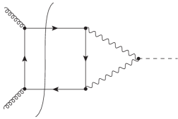
(a)

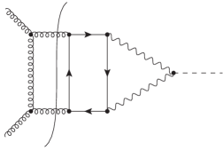
(b)

Figure 4: Examples of cut-diagrams contributing to the discontinuity for $0<s<m_{W,Z}^{2}$.

7 Conclusions

We computed the three-loop virtual contributions to next-to-leading order mixed QCD-electroweak corrections to Higgs boson production amplitude in the annihilation of two gluons $gg\to H$. The analytic result for the amplitude is obtained for arbitrary relation between the Higgs boson and the electroweak gauge boson masses. We computed the required integrals using the method of differential equations and obtained the boundary constants using the large-mass expansion valid in the limit $m_{H}\ll m_{W,Z}$. The finite part of the three-loop amplitude is written in terms of Goncharov polylogarithms and is easy to evaluate numerically.

To understand the impact of the mixed QCD-electroweak corrections on the Higgs boson production cross section, the virtual corrections computed in this paper will have to be combined with the real emission contributions of the type $gg\to Hg$, $qg\to Hq$ where, again, the Higgs boson couples to electroweak vector bosons. The computation of the relevant real emission amplitude is non-trivial as it involves two-loop box diagrams with both internal and external masses. Nevertheless, it is conceivable that, with the current computational technology, analytic results for these contributions can be obtained.

Appendix A Topologies

All the Feynman integrals appearing in the amplitude can be regrouped into three families, according to what propagators they feature. Table 2 shows the sets of inverse propagators for each family.

The parent topologies of each family are depicted in Figs. 5, 6 and 7. Solid lines are massive, wavy lines are massless.

Label	Families of denominators
	Planar (PP, Fig. 5)	Non-planar, A (NA, Fig. 6)	Non-planar, B (NB, Fig. 7)
$[1]$	$(k_{1})^{2}$	$(k_{2})^{2}$	$(k_{1})^{2}$
$[2]$	$(k_{2})^{2}$	$(k_{3})^{2}\,\,-\,\,M^{2}$	$(k_{2})^{2}$
$[3]$	$(k_{3})^{2}\,\,-\,\,M^{2}$	$(k_{1}+p_{3})^{2}$	$(k_{3})^{2}\,\,-\,\,M^{2}$
$[4]$	$(k_{1}+p_{3})^{2}$	$(k_{3}+p_{3})^{2}\,\,-\,\,M^{2}$	$(k_{1}+p_{3})^{2}$
$[5]$	$(k_{2}+p_{3})^{2}$	$(k_{3}-k_{2})^{2}$	$(k_{2}+p_{3})^{2}$
$[6]$	$(k_{3}+p_{3})^{2}\,\,-\,\,M^{2}$	$(k_{2}-k_{1})^{2}$	$(k_{3}+p_{3})^{2}\,\,-\,\,M^{2}$
$[7]$	$(k_{3}-k_{2})^{2}$	$(k_{3}-k_{1})^{2}$	$(k_{3}-k_{2})^{2}$
$[8]$	$(k_{2}-k_{1})^{2}$	$(k_{1}-p_{1})^{2}$	$(k_{2}-k_{1})^{2}$
$[9]$	$(k_{3}-k_{1})^{2}$	$(k_{2}-p_{1})^{2}$	$(k_{1}-p_{1})^{2}$
$[10]$	$(k_{1}-p_{1})^{2}$	$(k_{1}-k_{2}-p_{1})^{2}$	$(k_{3}-p_{1})^{2}$
$[11]$	$(k_{2}-p_{1})^{2}$	$(k_{1}-k_{2}+k_{3}+p_{3})^{2}$	$(k_{1}-k_{2}+k_{3}+p_{3})^{2}$
$[12]$	$(k_{3}-p_{1})^{2}$	$(k_{3}-k_{2}-p_{2})^{2}$	$(k_{2}-k_{1}-p_{2})^{2}$

Table 2: The three families of denominators appearing in the amplitude.

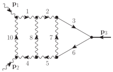
(a)

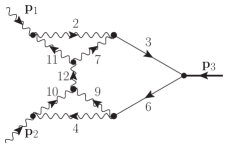
(b)

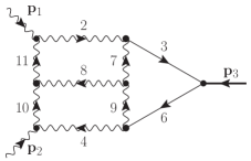
(c)

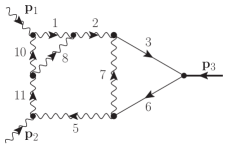
(d)

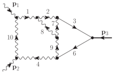
(e)

Figure 5: Planar parent topologies (PP).

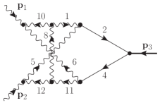
(a)

(b)

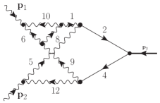
(c)

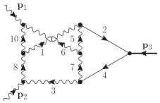
(d)

Figure 6: Non-planar A-type parent topologies (NA).

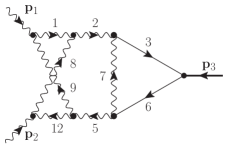
(a)

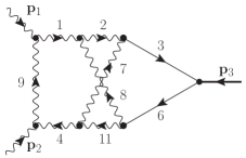
(b)

Figure 7: Non-planar B-type parent topologies (NB).

Appendix B Master integrals

The form factor $\mathcal{F}$ can be expressed in terms of 95 MIs, depicted in Figs. 8, 9 and 10.

A circled number besides the graph indicates that the corresponding denominator features in the numerator.

The MIs with an asterisk (^∗) do not contribute to the NLO form factor, but appear in the differential equations.

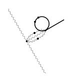
(a)

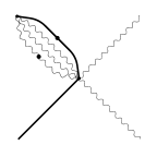
(b)

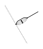
(c)

(d)

(e)

(f)

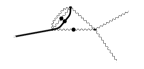
(g)

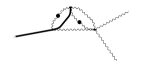
(h)

(i)

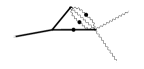
(j)

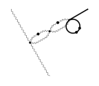
(k)

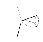
(l)

(m)

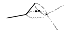
(n)

(o)

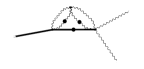
(p)

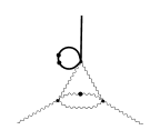
(q)

(r)

(s)

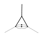
(t)

(u)

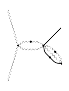
(v)

(w)

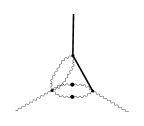
(x)

(y)

(z)

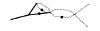
(aa)

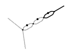
(ab)

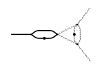
(ac)

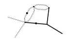
(ad)

Figure 8: Master Integrals (1/3).

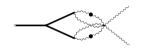
(a)

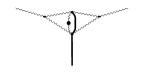
(b)

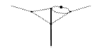
(c)

(d)

(e)

(f)

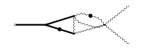
(g)

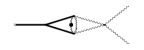
(h)

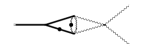
(i)

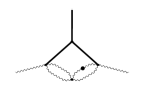
(j)

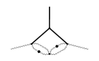
(k)

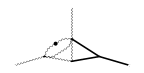
(l)

(m)

(n)

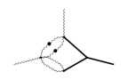
(o)

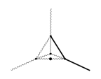
(p)

(q)

(r)

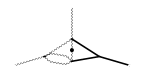
(s)

(t)

(u)

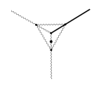
(v)

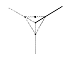
(w)

(x)

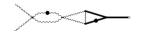
(y)

(z)

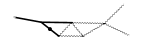
(aa)

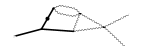
(ab)

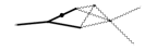
(ac)

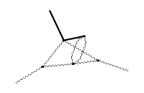
(ad)

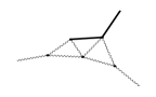
(ae)

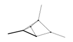
(af)

(ag)

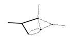
(ah)

(ai)

(aj)

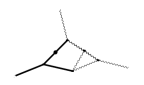
(ak)

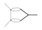
(al)

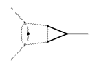
(am)

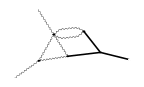
(an)

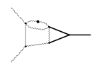
(ao)

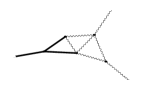
(ap)

Figure 9: Master Integrals (2/3).

(a)

(b)

(c)

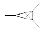
(d)

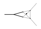
(e)

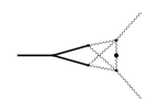
(f)

(g)

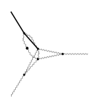
(h)

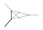
(i)

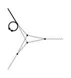
(j)

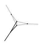
(k)

(l)

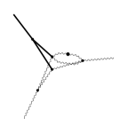
(m)

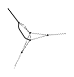
(n)

(o)

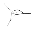
(p)

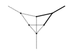
(q)

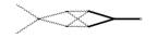
(r)

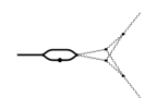
(s)

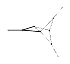
(t)

(u)

(v)

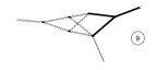
(w)

(x)

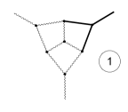
(y)

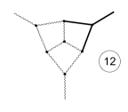
(z)

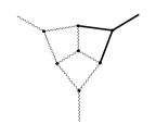
(aa)

(ab)

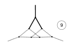
(ac)

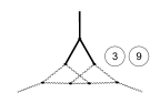
(ad)

(ae)

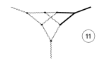
(af)

(ag)

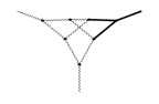
(ah)

Figure 10: Master Integrals (3/3).

References

- [1] C. Anastasiou, C. Duhr, F. Dulat, E. Furlan, T. Gehrmann, F. Herzog, A. Lazopoulos, and B. Mistlberger, High precision determination of the gluon fusion Higgs boson cross-section at the LHC, JHEP 05 (2016) 058, [arXiv:1602.0069].
- [2] Particle Data Group Collaboration, C. Patrignani et al., Review of Particle Physics, Chin. Phys. C40 (2016), no. 10 100001.
- [3] C. Anastasiou, R. Boughezal, and F. Petriello, Mixed QCD-electroweak corrections to Higgs boson production in gluon fusion, JHEP 04 (2009) 003, [arXiv:0811.3458].
- [4] U. Aglietti, R. Bonciani, G. Degrassi, and A. Vicini, Two-loop electroweak corrections to Higgs production in proton-proton collisions, in TeV4LHC Workshop: 2nd Meeting Brookhaven, Upton, New York, February 3-5, 2005, 2006. hep-ph/0610033.
- [5] U. Aglietti, R. Bonciani, G. Degrassi, and A. Vicini, Two loop light fermion contribution to Higgs production and decays, Phys. Lett. B595 (2004) 432–441, [hep-ph/0404071].
- [6] U. Aglietti, R. Bonciani, G. Degrassi, and A. Vicini, Master integrals for the two-loop light fermion contributions to and , Phys. Lett. B600 (2004) 57–64, [hep-ph/0407162].
- [7] M. Bonetti, K. Melnikov, and L. Tancredi, Two-loop electroweak corrections to Higgs–gluon couplings to higher orders in the dimensional regularization parameter, Nucl. Phys. B916 (2017) 709–726, [arXiv:1610.0549].
- [8] A. V. Kotikov, Differential equations method: New technique for massive Feynman diagrams calculation, Phys. Lett. B254 (1991) 158–164.
- [9] E. Remiddi, Differential equations for Feynman graph amplitudes, Nuovo Cim. A110 (1997) 1435–1452, [hep-th/9711188].
- [10] T. Gehrmann and E. Remiddi, Differential equations for two loop four point functions, Nucl. Phys. B580 (2000) 485–518, [hep-ph/9912329].
- [11] J. M. Henn, Multiloop integrals in dimensional regularization made simple, Phys. Rev. Lett. 110 (2013) 251601, [arXiv:1304.1806].
- [12] E. Remiddi and J. A. M. Vermaseren, Harmonic polylogarithms, Int. J. Mod. Phys. A15 (2000) 725–754, [hep-ph/9905237].
- [13] A. B. Goncharov, Polylogarithms in Arithmetic and Geometry, in Proceeding of the International Congress of Mathematicians, pp. 374–387, 1994.
- [14] J. Vollinga and S. Weinzierl, Numerical evaluation of multiple polylogarithms, Comput. Phys. Commun. 167 (2005) 177, [hep-ph/0410259].
- [15] A. von Manteuffel and C. Studerus, Reduze 2 - Distributed Feynman Integral Reduction, arXiv:1201.4330.
- [16] J. M. Henn, Lectures on differential equations for Feynman integrals, J. Phys. A48 (2015) 153001, [arXiv:1412.2296].
- [17] M. Argeri, S. Di Vita, P. Mastrolia, E. Mirabella, J. Schlenk, U. Schubert, and L. Tancredi, Magnus and Dyson Series for Master Integrals, JHEP 03 (2014) 082, [arXiv:1401.2979].
- [18] T. Gehrmann, A. von Manteuffel, L. Tancredi, and E. Weihs, The two-loop master integrals for , JHEP 06 (2014) 032, [arXiv:1404.4853].
- [19] R. N. Lee, Reducing differential equations for multiloop master integrals, JHEP 04 (2015) 108, [arXiv:1411.0911].
- [20] C. Meyer, Transforming differential equations of multi-loop Feynman integrals into canonical form, JHEP 04 (2017) 006, [arXiv:1611.0108].
- [21] L. Adams, E. Chaubey, and S. Weinzierl, Simplifying Differential Equations for Multiscale Feynman Integrals beyond Multiple Polylogarithms, Phys. Rev. Lett. 118 (2017), no. 14 141602, [arXiv:1702.0427].
- [22] N. Nielsen, Der Eulersche Dilogarithmus und seine Verallgemeinerungen, Nova Acta Leopoldina (Halle) 90 (1909), no. 123.
- [23] E. E. Kummer, Über die Transcendenten, welche aus wiederholten Integrationen rationaler Formeln entstehen, J. reine ang. Mathematik 21 (1840) 74–90; 193–225; 328–371.
- [24] T. Gehrmann and E. Remiddi, Two loop master integrals for 3 jets: The Planar topologies, Nucl. Phys. B601 (2001) 248–286, [hep-ph/0008287].
- [25] O. Gituliar and V. Magerya, Fuchsia: a tool for reducing differential equations for Feynman master integrals to epsilon form, Comput. Phys. Commun. 219 (2017) 329–338, [arXiv:1701.0426].
- [26] C. Meyer, Algorithmic transformation of multi-loop master integrals to a canonical basis with CANONICA, arXiv:1705.0625.
- [27] A. Primo and L. Tancredi, On the maximal cut of Feynman integrals and the solution of their differential equations, Nucl. Phys. B916 (2017) 94–116, [arXiv:1610.0839].
- [28] P. A. Baikov, Explicit solutions of the three loop vacuum integral recurrence relations, Phys. Lett. B385 (1996) 404–410, [hep-ph/9603267].
- [29] H. Frellesvig and C. G. Papadopoulos, Cuts of Feynman Integrals in Baikov representation, JHEP 04 (2017) 083, [arXiv:1701.0735].
- [30] J. Ablinger, J. Blumlein, and C. Schneider, Harmonic Sums and Polylogarithms Generated by Cyclotomic Polynomials, J. Math. Phys. 52 (2011) 102301, [arXiv:1105.6063].
- [31] A. von Manteuffel, R. M. Schabinger, and H. X. Zhu, The Complete Two-Loop Integrated Jet Thrust Distribution In Soft-Collinear Effective Theory, JHEP 03 (2014) 139, [arXiv:1309.3560].
- [32] V. A. Smirnov, Applied asymptotic expansions in momenta and masses, Springer Tracts Mod. Phys. 177 (2002) 1–262.
- [33] T. Gehrmann, T. Huber, and D. Maitre, Two-loop quark and gluon form-factors in dimensional regularisation, Phys. Lett. B622 (2005) 295–302, [hep-ph/0507061].
- [34] M. Steinhauser, MATAD: A Program package for the computation of MAssive TADpoles, Comput. Phys. Commun. 134 (2001) 335–364, [hep-ph/0009029].
- [35] S. Borowka, G. Heinrich, S. P. Jones, M. Kerner, J. Schlenk, and T. Zirke, SecDec-3.0: numerical evaluation of multi-scale integrals beyond one loop, Comput. Phys. Commun. 196 (2015) 470–491, [arXiv:1502.0659].
- [36] S. Borowka, G. Heinrich, S. Jahn, S. P. Jones, M. Kerner, J. Schlenk, and T. Zirke, pySecDec: a toolbox for the numerical evaluation of multi-scale integrals, arXiv:1703.0969.
- [37] S. Catani, The Singular behavior of QCD amplitudes at two loop order, Phys. Lett. B427 (1998) 161–171, [hep-ph/9802439].