TMCI and Space Charge

Abstract

Transverse mode-coupling instability (TMCI) is known to limit bunch intensity. Since space charge (SC) changes coherent spectra, it affects the TMCI threshold. Generally, there are only two types of TMCI with respect to SC: the vanishing type and the strong space charge (SSC) type. For the former, the threshold value of the wake tune shift is asymptotically proportional to the SC tune shift, as it was first observed twenty years ago by M. Blaskiewicz for exponential wakes. For the latter, the threshold value of the wake tune shift is asymptotically inversely proportional to the SC, as it was shown by one of the authors. In the presented studies of various wakes, potential wells, and bunch distributions, the second type of instability was always observed for cosine wakes; it was also seen for the sine wakes in the case of a bunch within a square potential well. The vanishing TMCI was observed for all other wakes and distributions we discuss in this paper: always for the negative wakes, and always, except the cosine wake, for parabolic potential wells. At the end of this paper, we consider high-frequency broadband wake, suggested as a model impedance for CERN SPS ring. As expected, TMCI is of the vanishing type in this case. Thus, SPS Q26 instability, observed at strong SC almost with the same bunch parameters as it would be observed without SC, cannot be TMCI.

I Introduction

The problems of coherent beam stability are known to be hard when the beam space charge (SC) has to be taken into account, which is necessary for low- and medium-energy hadron rings. So far the only universally accurate method available is macroparticle tracking; since the number of needed macroparticles per bunch may be up to a billion for reliable results, this method is very expensive in terms of CPU time. This is why analytical models are valuable: although each of them has limitations, they help build general understanding, providing important results within their areas of validity. Since these areas, as well as the models’ accuracy, are not always clear, the results of available analytical models should be compared whenever possible.

The transverse mode coupling instability (TMCI), also known as the strong head-tail instability, is one of the main intensity limitations of bunched beams in circular machines Chao (1993). The specifics and even existence of this instability for beams with strong space charge, i.e. when the SC tune shift exceeds the synchrotron tune, remained unclear for a rather long time. A breakthrough publication in this direction, authored by M. Blaskiewicz, appeared about twenty yeas ago Blaskiewicz (1998). A model of an AirBag bunch within a Square potential well (addressed here as the ABS model) was presented and analyzed there with the exponential wake and an arbitrary ratio of the SC tune shift to the synchrotron tune, or the space charge parameter. A method to extend this model to an arbitrary sum of exponential/oscillating wakes was also described. It was shown that for a wide range of the wake decay rate and the SC parameter the instability threshold grows with the latter. A qualitative explanation of why SC may work this way was suggested the next year Ng and Burov (1999). In 2009, a theory of head-tail instabilities with strong space charge (SSC) was presented in Refs. Burov (2009); Balbekov (2009). One of the authors of this paper speculated then that dependence of the TMCI threshold on the SC parameter might be non-monotonic, meaning that the threshold might start to decrease after a certain value of the SC tune shift. It was demonstrated that for the cosine wake this statement is true, but whether it is true for sign-constant wakes remained unclear. About a year ago, V. Balbekov confirmed his agreement Balbekov (2016a) with this hypothesis for the constant wake and the boxcar model (referred to as HP₀ distribution in this paper). Soon after that, however, he withdrew this result, claiming that for both ABS and boxcar models the threshold grows monotonically with the space charge parameter, showing no hint that this trend would change at a higher SC Balbekov (2016b, a, 2017a, 2017b). It has been also shown Balbekov (2017a) that for the cosine wake with the phase advance not exceeding $\pi$, the TMCI threshold monotonically increases with the SC parameter, similarly to the negative wakes.

In this paper, we are trying to get a better confidence and wider vision of the TMCI threshold versus the SC parameter for various wakes, potential wells and bunch longitudinal distributions. Our paper is a summary of results for several models.

We use two analytical approaches: the ABS of M. Blaskiewicz and the Strong Space Charge (SSC) theory of Ref. Burov (2009). While the ABS model can be applied for any SC strength, the SSC theory is applicable only when the SC tune shift sufficiently exceeds both the synchrotron tune and the coherent tune shift due to the wake. However, the SSC theory has an advantage in its applicability for any potential wells and longitudinal distributions, so the two approaches complement each other. Within the SSC approach, we examine first the square potential well with an arbitrary longitudinal distribution, and then the boxcar distribution for the parabolic potential well. The former of these we denote as SSCSW (strong space charge, square well), and to the latter we refer as the generalized Hofmann-Pedersen distribution of zeroth order, or SSCHP₀ model; the naming was suggested by Hofmann and Pedersen (1979).

In addition to SSCHP₀, we also consider elliptic arc and parabolic line densities for the same potential well, or SSCHP_1/2 and SSCHP₁ models. On top of that, TMCI for a Gaussian bunch at the strong space charge limit (SSCG) is discussed for various wakes.

Recently, the two-particle model for a bunch with SC and a constant wake has been suggested in Chin et al. (2016). We think that its main advantage, simplicity, is somewhat excessive for the specific problem under study, so we leave its possible application outside the framework of this paper.

For the negative exponential wakes our conclusion agrees with M. Blaskiewicz Blaskiewicz (1998) and the latest results of V. Balbekov Balbekov (2017a): SC always elevates the TMCI threshold; when the SC parameter is large, the threshold wake tune shift grows linearly with it. This result is also confirmed with all SSC models for the resistive wall wake.

For the cosine wakes and strong space charge, the situation is different. When SC is strong enough, it makes the beam less stable; the threshold is found to be inversely proportional to the SC parameter, provided that the wake phase advance is sufficiently large, $\omega\,\tau_{\mathrm{b}}>\pi$. However, for the same wake with a small or moderate SC parameter, the thresholds typically show some growth with SC, thus confirming the hypothesis of Ref. Burov (2009) about non-monotonic dependence of the TMCI threshold on the SC parameter for oscillating wakes. When the wake oscillations are not well-pronounced (either the phase advance is insufficient, $\omega\,\tau_{\mathrm{b}}<\pi$, or the wake oscillations are overshadowed by their exponential decay), the TMCI vanishes at the SSC limit, as expected.

For the sine wake at SSC, results for the square and parabolic potential wells were found to be qualitatively different. For the SSCSW model the TMCI behaves in a similar manner as for the cosine wake, but every mode coupling is followed by its decoupling at higher wake amplitude. Contrary to that, the modes never couple for the SSCHP₀ model; they either cross or approach-divert, as if the instability is prohibited for this case. For more realistic SSCHP_1/2,1 and SSCG models, we found that there is no TMCI either, even without any crossings or approach-diverts. Thus, from our numerical results we conclude that TMCI vanishes for the parabolic potential well and the sine wake.

It will be shown in Section II that there are only two types of TMCI with respect to the SC. The first one, called here vanishing TMCI, is such that its threshold wake tune shift asymptotically scales as the SC tune shift. For this sort of instability, there is an absolute threshold of the wake amplitude, inversely proportional to the transverse emittance: below this threshold, the beam is stable for any number of particles. For the second type of TMCI, which we call SSC TMCI, the wake threshold asymptotically drops in the inverse proportion to the SC tune shift. No other type of the asymptotic threshold behavior is possible.

I.1 Article structure

The paper is structured as follows. First, Sec. II summarizes the SSC and ABS main formulas for a single bunch at zero chromaticity for the reader’s convenience. Modes for the no-wake case, or the SSC harmonics, are presented in the subsection II.1 for all strong space charge models. Subsection II.2 describes the airbag model including the solution for a no-wake case. Two Sections III and IV are dedicated to the negative (delta-functional, constant, step-function, exponential and resistive wall) and oscillating (sine, cosine and resonator) wake functions respectively. In subsection IV.3, dedicated to resonator wakes, we compare SSC theory with the results of simulations Blaskiewicz (2012). The last subsection IV.4 presents TMCI threshold versus space charge parameter for the high-frequency broadband wake suggested for CERN SPS ring, using for that the ABS model; these results are compared with simulations of Ref. Quatraro and Rumolo (2010). Appendix A contains the expressions of the wake matrix elements $\widehat{\mathrm{W}}_{lm}$ for the SSCHP₀ and details of their computation for other models. Appendix B provides the reader with details on the exponential and trigonometric wakes for the ABS model. Since some of the results are qualitatively similar to each other, the last complementary Appendix C includes all bunch spectra for SSC models not presented into the main text.

II Analytical models

II.1 Strong space charge theory

In this subsection, we recall the main formulas of the SSC theory Burov (2009), which accuracy was verified by multiparticle tracking simulations of Ref Macridin et al. (2015). Consider a single bunch with a longitudinal distribution function $f(\tau,\mathrm{v})$, where $\tau$ is the position along the bunch, and $\mathrm{v}$ is the particle longitudinal velocity, $\mathrm{v}=\mathrm{d}\tau/\mathrm{d}\theta$. Both the position $\tau$ and the time $\theta$ are measured in radians. For zero wake, transverse modes satisfy an ordinary differential equation with zero-derivative boundary conditions, which composes a standard Sturm-Liouville (S-L) problem,

$$\left\{\begin{array}[]{l}\displaystyle\frac{1}{Q_{\text{eff}}(\tau)}\frac{\mathrm{d}}{\mathrm{d}\tau}\left[u^{2}(\tau)\frac{\mathrm{d}\,Y(\tau)}{\mathrm{d}\tau}\right]+\nu\,Y(\tau)=0,\\[14.22636pt] \displaystyle\left.\frac{\mathrm{d}}{\mathrm{d}\tau}\,Y(\tau)\right|_{\tau=\pm\infty}=0.\end{array}\right.$$ (1)

Solutions of this problem constitute an orthogonal basis, which when normalized will be referred to as the SSC harmonics $[\nu_{k},Y_{k}(\tau)]$:

$$\int_{\text{SB}}\rho(\tau)\,Y_{l}(\tau)\,Y_{m}(\tau)\,\mathrm{d}\tau=\delta_{lm},$$ (2)

with $\rho(\tau)$ being the normalized line density

$$\rho(\tau)=\int f(\tau,\mathrm{v})\,\mathrm{d}\mathrm{v}:\qquad\int_{\text{SB}}\rho(\tau)\,\mathrm{d}\tau=1.$$ (3)

The SB integration limit indicates integration along the bunch length of the single bunch. The temperature function $u^{2}(\tau)$ is the local average of the longitudinal velocity squared,

$$u^{2}(\tau)=\int f(\tau,\mathrm{v})\,\mathrm{v}^{2}\,\mathrm{d}\mathrm{v}\,\bigg{/}\,\rho(\tau).$$ (4)

$Q_{\text{eff}}$ is the effective space charge tune shift at the given position along the bunch,

$$Q_{\text{eff}}(\tau)=Q_{\text{eff}}(0)\,\frac{\rho(\tau)}{\rho(0)},$$ (5)

where “effective” means the transverse average at the given position $\tau$ along the bunch. If the transverse distribution is Gaussian, the effective space charge tune shift is $\approx 0.52$ of its value at the beam axis.

The wake function $W(\tau)$ modifies the collective dynamics as follows:

$$\frac{1}{Q_{\text{eff}}(\tau)}\frac{\mathrm{d}}{\mathrm{d}\tau}\left[u^{2}(\tau)\frac{\mathrm{d}\,\mathcal{Y}(\tau)}{\mathrm{d}\tau}\right]+\Delta q\,\mathcal{Y}(\tau)=\kappa\,\widehat{\mathrm{W}}\,\mathcal{Y}(\tau),$$ (6)

with

$$\widehat{\mathrm{W}}\,\mathcal{Y}(\tau)=\int_{\tau}^{\infty}W(\tau-\sigma)\,\rho(\sigma)\,\mathcal{Y}(\sigma)\,\mathrm{d}\sigma,$$ (7)

and

$$\kappa=N_{\text{b}}\,\frac{r_{0}R_{0}}{4\,\pi\,\gamma\,\beta^{2}\,Q_{\beta}}.$$ (8)

Here $N_{\text{b}}$ is the number of particles per bunch, $r_{0}$ is the particle classical radius, $R_{0}=C_{0}/(2\pi)$ is the average accelerator ring radius, $Q_{\beta}$ is the bare betatron tune, $\gamma$ is the Lorentz factor and $\beta$ is the ratio of particle velocity to the speed of light. Zero-derivative boundary condition, as in Eq. (1), is assumed. Equation (6) implies zero chromaticity, which is always the case in this paper.

Note that this eigensystem problem has a special scaling with respect to the SC. If $\{Y,\Delta q\}$ are an eigenfunction and eigenvalue for certain SC tune shift $Q_{\text{eff}}$ and wake $W$, then for $\alpha$ times larger SC, $\alpha\,Q_{\text{eff}}$, and $\alpha$ times smaller wake, $W/\alpha$, the eigenvalues scale as $\Delta q/\alpha$, while the eigenfunctions $Y$ remain the same. Consequently, the instability threshold, if there is any, scales inversely proportional to the SC tune shift $\kappa W_{\mathrm{th}}\propto 1/Q_{\text{eff}}(0)$. That sort of instabilities, seen within the SSC asymptotic approach, we call SSC TMCI. When modes of Eq. (6) never couple, it does not mean that TMCI is impossible. Instead, it means that TMCI can only be outside the SSC applicability area, when some of wake tune shifts are comparable with the SC tune shift of the core particles, $Q_{\text{eff}}(0)$. When the SC-asymptotic of the TMCI threshold is considered, $Q_{\text{eff}}(0)$ exceeds all other tune shifts, which means that the TMCI threshold, if it does exist at all, asymptotically has to be proportional to the SC tune shift, $\kappa W_{\mathrm{th}}\propto Q_{\text{eff}}(0)$. This type of TMCI we call vanishing, since it cannot be seen at SSC. An interesting feature of the vanishing type is that in this case there is an absolute threshold of the wake amplitude: if the wake is smaller that this threshold, the beam is stable for any number of particles. It is straightforward to show that the absolute wake threshold is inversely proportional to the transverse emittance and average beta-function. Let us stress one more time, that except these two types of TMCI no other type is possible, whatever are wakes, potential wells and bunch distributions.

Equation (6) can be solved by means of expansion over the orthonormal basis of its zero-wake eigenfunctions, or the SSC harmonics,

$$\mathcal{Y}_{k}(\tau)=\sum_{i=0}^{\infty}\mathbf{C}^{(k)}_{i}Y_{i}(\tau)$$ (9)

leads to the eigenvalue problem

$$\mathbf{M}\cdot\mathbf{C}^{(k)}=\Delta q_{k}\mathbf{C}^{(k)},\qquad\mathbf{M}_{lm}=\nu_{l}\,\delta_{lm}+\kappa\,\widehat{\mathrm{W}}_{lm},$$ (10)

with matrix elements of the wake operator being

$$\widehat{\mathrm{W}}_{lm}=\int_{-\infty}^{\infty}\int_{\tau}^{\infty}W(\tau-\sigma)\,\rho(\tau)\,\rho(\sigma)\,Y_{l}(\tau)\,Y_{m}(\sigma)\,\mathrm{d}\,\sigma\,\mathrm{d}\,\tau.$$ (11)

The eigenvalues $\Delta q_{k}$ constitute the bunch spectrum, and once they have been determined we look for imaginary values corresponding to coherent growth rates of instabilities. Real parts of $\Delta q_{k}$ correspond to coherent tune shifts and are equal to $\nu_{k}$ for the no-wake case. In order to study the effect of the wake on the bunch stability, we introduce a parameter combining the intensity and the wake amplitude, $W_{0}$,

$$\chi^{*}=\frac{\kappa\,W_{0}\,Q_{\text{eff}}(0)}{Q_{\text{s}}^{2}}.$$ (12)

As it was demonstrated by V. Balbekov Balbekov (2017a), the expansion over the SSC harmonics may have a poor convergence, so that the numerically obtained instability threshold is very sensitive to the accuracy of the matrix elements computation and the number of harmonics taken into account. In order to distinguish the illusory, purely numerical, threshold from the real one, two things are required: a large number of basis harmonics and high accuracy of the computed matrix elements. To provide that, we considered two different distributions with constant line density (SSCSW and SSCHP₀ defined below), where the matrix elements can be computed analytically, thus minimizing numerical errors up to machine precision and justifying the inclusion of large number of modes into analysis. Analytical expressions for the matrix elements $\widehat{\mathrm{W}}_{lm}$ are provided in Appendix A.1.

In order to compare results of these rather simplified models, some cases were considered with a parabolic potential well and smoother bunch distributions, including the Gaussian one. The eigensystems for the first 40 modes were found using Wolfram Mathematica 11.0. Then, the matrix elements were calculated using numerical integration (see Appendix A.2 for details). Below we give definitions of all our SSC models and describe SSC harmonics.

II.1.1 Square potential well

Our first SSC model relates to a bunch in the Square potential Well (SSCSW). In this case the distribution function is factorized

$$f_{\text{sw}}(\tau,\mathrm{v})=\frac{1}{\tau_{\mathrm{b}}}\,\text{H}\left[1-4\,\frac{\tau^{2}}{\tau_{\mathrm{b}}^{2}}\right]\mathrm{V}(\mathrm{v}).$$ (13)

Below we omit the Heaviside function, assuming that all bunch related functions are defined on its length, $|\tau|\leq\tau_{\mathrm{b}}/2$. The average square of velocity is position-independent,

$$u_{\text{sw}}^{2}(\tau)\equiv\mathrm{v}_{\mathrm{b}}^{2}.$$ (14)

Then, the equation for the SSC harmonics can be written as

$$0=\nu_{k}\,Y_{k}^{\text{sw}}(\tau)+\frac{\mathrm{v}_{\mathrm{b}}^{2}}{Q_{\text{eff}}(0)}\frac{\mathrm{d}}{\mathrm{d}\tau}\left[\frac{\mathrm{d}}{\mathrm{d}\tau}\,Y_{k}^{\text{sw}}(\tau)\right].$$ (15)

With $\tau$ measured in units of $\tau_{\mathrm{b}}$ and $\nu$ in units of $Q_{s}^{2}/Q_{\text{eff}}(0)\equiv\pi^{2}\mathrm{v}_{\mathrm{b}}^{2}/[\tau_{\mathrm{b}}^{2}Q_{\text{eff}}(0)]$, it reduces to

$$\left\{\begin{array}[]{l}\displaystyle Y^{\prime\prime}(\tau)+\pi^{2}\nu\,Y(\tau)=0,\\[7.11317pt] Y^{\prime}(\pm 1/2)=0.\end{array}\right.$$ (16)

This S-L problem yields the eigenvalues as integers squared,

$$\nu_{k}^{\text{sw}}=\left\{k^{2}\,|\,k\in\mathbb{Z}\right\}=\left\{0,1,4,9,25,36,\ldots\right\}.$$ (17)

The set of eigenfunctions, normalized according to the general SSC harmonics orthonormalization rule (3), consists of the constant 0-th mode, $Y^{\text{sw}}_{0}=1$, and a sequence of cosine and sine functions (see Fig. 1)

$$Y_{k}^{\text{sw}}(\tau)=\sqrt{2-\delta_{0k}}\times\left\{\begin{array}[]{lll}\displaystyle\cos(\pi\,k\,\tau),&&k\text{ is even},\\[7.11317pt] \displaystyle\sin(\pi\,k\,\tau),&&k\text{ is odd}.\end{array}\right.$$ (18)

II.1.2 Hofmann-Pedersen distribution

Another SSC model, where matrix elements for some wakes can be analytically calculated, is a bunch with a constant line density inside a parabolic potential well. Following M. Blaskiewicz, this distribution was previously referred as a boxcar, but since more than one of our models have a boxcar, or constant, line density, in order to avoid confusions, we refer to it as the $\text{HP}_{0}$ model, or zeroth Hofmann-Pedersen distribution. Its phase space density can be written as a function of the Hamiltonian

$$f_{\text{HP}_{0}}(\tau,\mathrm{v})=\frac{2}{\pi\,\tau_{\mathrm{b}}\mathrm{v}_{\mathrm{b}}}\,\left(1-\frac{\mathcal{H}}{\mathcal{H}_{b}}\right)^{-1/2}\text{H}\left[1-\frac{\mathcal{H}}{\mathcal{H}_{b}}\right],$$ (19)

where

$$\frac{\mathcal{H}}{\mathcal{H}_{b}}=4\,\left[\left(\frac{\tau}{\tau_{\mathrm{b}}}\right)^{2}+\left(\frac{\mathrm{v}}{\mathrm{v}_{\mathrm{b}}}\right)^{2}\right],$$ (20)

$\mathcal{H}_{b}$ is the Hamiltonian of the boundary particle, and, we omit the Heaviside step function understanding the domain where $f_{\text{HP}_{0}}(\tau,\mathrm{v})$ is properly defined.

This notation assumes a generalized Hofmann-Pedersen distribution of the $n$-th order

$$f_{\text{HP}_{n}}(\tau,\mathrm{v})=\frac{2\,(2\,n+1)}{\pi\,\tau_{\mathrm{b}}\mathrm{v}_{\mathrm{b}}}\left(1-\frac{\mathcal{H}}{\mathcal{H}_{b}}\right)^{n-1/2},$$ (21)

for $n=0,\frac{1}{2},1,\frac{3}{2},\ldots$. Independently of the order, the temperature function is parabolic

$$u_{\text{HP}_{n}}^{2}(t)=\frac{\mathrm{v}_{\mathrm{b}}^{2}}{8(n+1)}\left(1-4\,\frac{\tau^{2}}{\tau_{\mathrm{b}}^{2}}\right),$$ (22)

while the line density is given by

$$\rho_{\text{HP}_{n}}(t)=\frac{2\,\Gamma[n+3/2]}{\tau_{\mathrm{b}}\sqrt{\pi}\,\Gamma[n+1]}\left(1-4\,\frac{\tau^{2}}{\tau_{\mathrm{b}}^{2}}\right)^{n},$$ (23)

so the conventional Hofmann-Pedersen distribution Hofmann and Pedersen (1979), with its parabolic line density, can be addressed as $f_{\text{HP}_{1}}$.

In this paper, in addition to the SSCHP₀ case which admits the analytical expressions of the matrix elements, we also consider more realistic models with $n=1/2,1$ (referred to as SSCHP_1/2,1 respectively) for a bunch in a parabolic potential well, where integrals of the matrix elements were computed numerically; the SSCHP_1/2 model sometimes is referred as the waterbag distribution. Table 1 contains exact expressions for longitudinal distribution, temperature and density functions for all models under consideration.

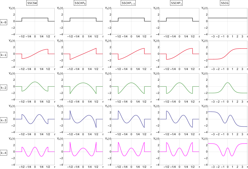
Figure 1: First five SSC harmonics $Y_{k}(\tau)$ for a bunch in a square potential well, bunch in a parabolic potential well (generalized Hofmann-Pedersen distributions with $n=0,1/2,1$) and the Gaussian bunch. The harmonics are presented in dimensionless units: $\tau$ is measured in units of $\tau_{\mathrm{b}}$ or in units of $\sigma_{\mathrm{b}}$ for the SSCG case.

Table 1: Longitudinal distribution function $f(\tau,\mathrm{v})$, the average of the longitudinal velocity squared $u^{2}(\tau)$, and, the normalized line density $\rho(\tau)$ for SSC models; last row shows graphs of the line density in dimensionless units.

	SSCSW	SSCHP0	SSCHP1/2	SSCHP1	SSCG
$f(\tau,\mathrm{v})$	$\displaystyle\frac{1}{\tau_{\mathrm{b}}}\text{H}\left[1-4\,\frac{\tau^{2}}{\tau_{\mathrm{b}}^{2}}\right]\mathrm{V}(\mathrm{v})$	$\displaystyle\frac{2}{\pi\,\tau_{\mathrm{b}}\mathrm{v}_{\mathrm{b}}}\left(1-\frac{\mathcal{H}}{\mathcal{H}_{b}}\right)^{-1/2}$	$\displaystyle\frac{4}{\pi\,\tau_{\mathrm{b}}\mathrm{v}_{\mathrm{b}}}\text{H}\left[1-\frac{\mathcal{H}}{\mathcal{H}_{b}}\right]$	$\displaystyle\frac{6}{\pi\,\tau_{\mathrm{b}}\mathrm{v}_{\mathrm{b}}}\left(1-\frac{\mathcal{H}}{\mathcal{H}_{b}}\right)^{1/2}$	$\displaystyle\frac{e^{-(\tau^{2}/\sigma_{\mathrm{b}}^{2}+\mathrm{v}^{2}/\mathrm{v}_{\mathrm{b}}^{2})/2}}{2\,\pi\,\sigma_{\mathrm{b}}\mathrm{v}_{\mathrm{b}}}$
$u^{2}(\tau)$	$\displaystyle\mathrm{v}_{\mathrm{b}}^{2}\equiv\int_{\text{SB}}\mathrm{v}^{2}\,\mathrm{V}(\mathrm{v})\,\mathrm{d}\mathrm{v}$	$\displaystyle\frac{\mathrm{v}_{\mathrm{b}}^{2}}{8}\,\left(1-4\,\frac{\tau^{2}}{\tau_{\mathrm{b}}^{2}}\right)$	$\displaystyle\frac{\mathrm{v}_{\mathrm{b}}^{2}}{12}\,\left(1-4\,\frac{\tau^{2}}{\tau_{\mathrm{b}}^{2}}\right)$	$\displaystyle\frac{\mathrm{v}_{\mathrm{b}}^{2}}{16}\,\left(1-4\,\frac{\tau^{2}}{\tau_{\mathrm{b}}^{2}}\right)$	$\displaystyle\mathrm{v}_{\mathrm{b}}^{2}$
$\rho(\tau)$	$\displaystyle\frac{1}{\tau_{\mathrm{b}}}$	$\displaystyle\frac{1}{\tau_{\mathrm{b}}}$	$\displaystyle\frac{4}{\pi\,\tau_{\mathrm{b}}}\sqrt{1-4\,\frac{\tau^{2}}{\tau_{\mathrm{b}}^{2}}}$	$\displaystyle\frac{3}{2\,\tau_{\mathrm{b}}}\left(1-4\,\frac{\tau^{2}}{\tau_{\mathrm{b}}^{2}}\right)$	$\displaystyle\frac{e^{-\tau^{2}/(2\,\sigma_{\mathrm{b}}^{2})}}{\sqrt{2\,\pi}\,\sigma_{\mathrm{b}}}$

The equation for SSC harmonics can be conveniently written in the normalized variables, when $\tau$ is measured in units of $\tau_{\mathrm{b}}$ and $\nu$ in units of $\mathrm{v}_{\mathrm{b}}^{2}/[\tau_{\mathrm{b}}^{2}Q_{\text{eff}}(0)]$,

$$\left\{\begin{array}[]{l}\displaystyle Y^{\prime\prime}-\frac{8\,\tau\,Y^{\prime}}{1-4\,\tau^{2}}+\frac{8\,\nu\,(n+1)\,Y}{(1-4\,\tau^{2})^{1-n}}=0,\\[14.22636pt] \displaystyle Y^{\prime}(\pm 1/2)=0.\end{array}\right.$$ (24)

Note that $\nu$ is measured in different units in SSCSW and SSCHP; this choice was made in order to have first eigenvalues $\nu_{1}\approx 1$ for all the models (for SSCSW and SSCHP₀ $\nu_{1}=1$) which simplifies the comparison.

When $n=0$, the S-L problem (24) doesn’t have solutions, due to the singularities at $\tau=\pm 0.5$. One way to overcome this problem is to add a small regularization term $\epsilon>0$,

$$Y^{\prime\prime}(\tau)-\frac{8\,\tau}{1+\epsilon-4\,\tau^{2}}\,Y^{\prime}(\tau)+\frac{8\,\nu}{1+\epsilon-4\,\tau^{2}}\,Y(\tau)=0,$$ (25)

thus removing the singularity within the same bunch length $[-0.5;0.5]$. With this regularization, the S-L solutions do exist, and, as $\epsilon\rightarrow 0$, the eigenvalues converge to the triangular numbers

$$\nu_{k}^{\text{HP}_{0}}=\left\{k\,(k+1)/2\,|\,k\in\mathbb{Z}\right\}=\left\{0,1,3,6,10,\ldots\right\}.$$ (26)

The eigenfunctions converge to functions proportional to the Legendre polynomials $P_{k}(\tau)$,

$$Y_{k}^{\text{HP}_{0}}(\tau)=(-1)^{\left\lfloor{k/2}\right\rfloor}\sqrt{2\,k+1}\,P_{k}(2\,\tau)$$ (27)

where the floor function $\left\lfloor n\right\rfloor$ is the integer part of $n$. The $(-1)^{\left\lfloor k/2\right\rfloor}$ factor guarantees that each even (odd) harmonic has cosine-like (sine-like) properties at the origin, see Eq. (28).

Another way to find eigenvalues is to look for an even and odd functions with

$$\left\{\begin{array}[]{l}Y\phantom{{}^{\prime}}(0)>0,\\ Y^{\prime}(0)=0,\end{array}\right.\qquad\text{or}\qquad\left\{\begin{array}[]{l}Y\phantom{{}^{\prime}}(0)=0,\\ Y^{\prime}(0)>0,\end{array}\right.$$ (28)

respectively. When the small regularization term $\epsilon>0$, the derivatives $Y^{\prime}(\pm 0.5)$ vanish for the same triangular values, $\nu_{k}^{\text{HP}_{0}}$. With $\epsilon=0$, only the triangular eigenvalues $\nu=k(k+1)/2$ yield the solutions, remaining finite at the bunch edges $\tau=\pm 0.5$.

The first ten numerically obtained values of $\nu_{k}$ for SSCHP_1/2,1 are given in Table 2 and first five harmonics for all cases are presented in Fig. 1.

Table 2: First ten eigenvalues $\nu_{k}$ for SSC models: bunch inside a square (SSCSW) and parabolic (SSCHP_0,1/2,1) potential wells, and, Gaussian bunch (SSCG).

$k$	SSCSW	SSCHP0	SSCHP1/2	SSCHP1	SSCG
0	0	0	0	0	0
1	1	1	1.1002	1.1555	1.342
2	4	3	3.378	3.5910	4.3245
3	9	6	6.8078	7.2713	8.8978
4	16	10	11.386	12.1905	15.0531
5	25	15	17.1115	18.3465	22.7868
6	36	21	23.9837	25.7383	32.0966
7	49	28	32.0023	34.3653	42.9817
8	64	36	41.1672	44.2272	55.441
9	81	45	51.4783	55.3235	69.474

II.1.3 Gaussian bunch

The last strong space charge case we present is the model of a thermalized beam with Gaussian distribution function (SSCG):

$$f_{\text{G}}(\tau,\mathrm{v})=\frac{1}{2\,\pi\,\sigma_{\mathrm{b}}\mathrm{v}_{\mathrm{b}}}\exp\left[-\frac{\tau^{2}}{2\,\sigma_{\mathrm{b}}}-\frac{\mathrm{v}^{2}}{2\,\mathrm{v}_{\mathrm{b}}}\right].$$ (29)

The normalized line density is simply a Gaussian distribution

$$\rho_{\text{G}}(\tau)=\frac{1}{\sqrt{2\,\pi}\sigma_{\mathrm{b}}}\exp\left[-\frac{\tau^{2}}{2\,\sigma_{\mathrm{b}}}\right],$$

and as in the case of SSCSW the average square of velocity is constant along the bunch

$$u_{\text{G}}^{2}(\tau)=\mathrm{v}_{\mathrm{b}}^{2}.$$ (30)

Using the similar normalized variables as for the SSCHP cases, where $\tau$ is measured in units of $\sigma_{\mathrm{b}}$ and $\nu$ in units of $Q_{s}^{2}/Q_{\text{eff}}(0)\equiv\mathrm{v}_{\mathrm{b}}^{2}/[\sigma_{\mathrm{b}}^{2}Q_{\text{eff}}(0)]$, the eigenfunction equation for transverse bunch oscillations is

$$\left\{\begin{array}[]{l}\displaystyle Y^{\prime\prime}(\tau)+\nu\,e^{-\tau^{2}/2}\,Y(\tau)=0,\\[7.11317pt] Y^{\prime}(\pm\infty)=0.\end{array}\right.$$ (31)

Below, we will adopt the convention that for all practical purposes the bunch length is defined as $\tau_{\mathrm{b}}=3\,\sigma_{\mathrm{b}}$. The first 10 numerically obtained eigenvalues $\nu_{k}$ are listed in the Table 2 and plots of first few eigenfunctions are given in Fig. 1.

II.2 Airbag in a square well

In addition to SSC cases, we consider the airbag longitudinal distribution inside a square well, abbreviated as ABS (AirBag Square well) model,

$$f_{\mathrm{ABS}}(\tau,\mathrm{v})\propto\left[\delta(\mathrm{v}-\mathrm{v}_{0})+\delta(\mathrm{v}+\mathrm{v}_{0})\right]\text{H}\left[1-4\,\frac{\tau^{2}}{\tau_{\mathrm{b}}^{2}}\right],$$ (32)

suggested by M. Blaskiewicz Blaskiewicz (1998). The ABS model allows the bunch spectrum to be determined for a wide class of wake functions in the presence of arbitrary space charge tune shift without requiring the expansion in basis functions, thereby avoiding convergence difficulties.

It is convenient to take for this model the following convention $\tau\in[-\tau_{\mathrm{b}}/2;\tau_{\mathrm{b}}/2]$ for the position along the bunch, where all particles move with the same absolute value of the velocity, $\mathrm{d}\,\tau/\mathrm{d}\theta=\pm\mathrm{v}_{0}$. Transverse offsets in the two fluxes of particles $X_{\pm}(\theta,\tau)$ can be looked for as

$$X_{\pm}(\theta,\tau)=e^{-i\,(Q_{\beta}+\Delta Q_{k})\theta}x_{\pm}(\tau)$$ (33)

where $Q_{\beta}$ is the bare betatron tune and $\Delta Q_{k}$ is the tune shift to be found. Then, equations for the amplitudes along the bunch $x_{\pm}(\tau)$ are given by

$$\frac{\mathrm{d}\,x_{+}}{\mathrm{d}\tau} = \frac{i}{\mathrm{v}_{0}}\left[\left(\frac{\Delta Q_{\mathrm{sc}}}{2}+\Delta Q_{k}\right)x_{+}-\frac{\Delta Q_{\mathrm{sc}}}{2}\,x_{-}-F\right],\qquad$$ (34)

$$\frac{\mathrm{d}\,x_{-}}{\mathrm{d}\tau} = \frac{i}{\mathrm{v}_{0}}\left[\frac{\Delta Q_{\mathrm{sc}}}{2}\,x_{+}-\left(\frac{\Delta Q_{\mathrm{sc}}}{2}+\Delta Q_{k}\right)x_{-}+F\right],\qquad$$ (35)

with the boundary conditions

$$\begin{array}[]{c}x_{+}(\tau_{\mathrm{b}}/2)=x_{-}(\tau_{\mathrm{b}}/2),\\[5.69046pt] x_{+}(-\tau_{\mathrm{b}}/2)=x_{-}(-\tau_{\mathrm{b}}/2).\end{array}$$ (36)

The force is defined by a wake function

$$F(\tau)=\kappa\,\int_{\tau}^{\tau_{\mathrm{b}}/2}W(\tau-\sigma)\,\overline{x}(\sigma)\,\mathrm{d}\sigma$$ (37)

and satisfies an integro-differential equation:

$$\frac{\mathrm{d}\,F(\tau)}{\mathrm{d}\tau}=-\kappa\,W(0)\,\overline{x}(\tau)+\kappa\,\int_{\tau}^{\tau_{\mathrm{b}}/2}\frac{\partial}{\partial\tau}W(\tau-\sigma)\overline{x}(\sigma)\,\mathrm{d}\sigma$$ (38)

with $\overline{x}=(x_{+}+x_{-})/2$. For a wake function in the form

$$W(\tau)=-W_{0}\,\sum_{k=1}^{n}C_{k}\,e^{\alpha_{k}\,\tau}$$ (39)

the force is

$$F=\sum_{k=1}^{n}F_{k}=-\kappa\,W_{0}\sum_{k=1}^{n}C_{k}\int_{\tau}^{\tau_{\mathrm{b}}/2}e^{\alpha_{k}(\tau-\sigma)}\,\overline{x}(\sigma)\,\mathrm{d}\sigma,$$ (40)

and for every $k=1,\ldots,n$,

$$\frac{\mathrm{d}\,F_{k}(\tau)}{\mathrm{d}\tau}=\frac{\kappa\,W_{0}}{2}\,C_{k}(x_{+}+x_{-})+\alpha_{k}\,F_{k},$$ (41)

with $F_{k}(\tau_{\mathrm{b}}/2)=0$.

Measuring $\tau$ in units of $\tau_{\mathrm{b}}$ and defining

$$f(\tau)=F(\tau)/Q_{\text{s}}$$ (42)

where $Q_{\text{s}}=\pi\,\mathrm{v}_{0}/\tau_{\mathrm{b}}$ is the synchrotron tune, Eqs. (34,35) and (41) can be presented as a set of ordinary linear homogeneous differential equations,

$$\frac{\mathrm{d}\,\mathrm{U}}{\mathrm{d}\tau}=\mathrm{M}\,\mathrm{U},$$ (43)

with boundary conditions

$$f_{k}(1/2) = 0,$$ (44)

$$x_{+}(1/2) = x_{-}(1/2),$$ (45)

$$x_{+}(-1/2) = x_{-}(-1/2),$$ (46)

where the vector $\mathrm{U}=(x_{+},x_{-},f_{1},f_{2},\ldots)$ has $n+2$ components and the matrix $\mathrm{M}$ is combined from the coefficients of Eqs. (34,35,41). To solve this set of equations, we suggest an algorithm different from one applied by M. Blaskiewicz.

The differential Eq. (43), first, can be transformed into a difference one,

$$\mathrm{U}_{n+1}-\mathrm{U}_{n}=\Delta\tau\,\mathrm{M}\,\mathrm{U}_{n}.$$ (47)

Choosing the number of steps to be $n=2^{m}$ and $\Delta\tau=1/2^{m}$, one has

$$\mathrm{U}_{0}\equiv\mathrm{U}(-1/2)=\left(\frac{1}{2^{m}}\,\mathrm{M}+\mathrm{I}\right)^{-2^{m}}\,\mathrm{U}_{n},$$ (48)

where $\mathrm{U}_{0}$ and $\mathrm{U}_{n}$ are values of $\mathrm{U}$ at the tail and the head of the bunch respectively, and, according to the boundary conditions (44–46)

$$\mathrm{U}_{n}\equiv\mathrm{U}(1/2)=(1,1,0,0,\ldots,0).$$

Those values of $\Delta Q_{k}$, with which the boundary condition at the tail of the bunch is satisfied, i.e.

$$x_{+}^{(0)}-x_{-}^{(0)}=0,$$ (49)

constitute the bunch spectrum; they can be found by a proper scan of the complex plane of $\Delta Q_{k}$. However, for the instability thresholds, it is sufficient to scan only real $\Delta Q_{k}$: the threshold can be detected as reduction of the number of these real modes by two.

This algorithm proves to be extremely time-efficient; the solution always converges with the number of intervals $1/\Delta\tau$, while the CPU time grows only logarithmically, $\propto\log_{2}(1/\Delta\tau)=m$.

For the no-wake case, the ABS spectrum is calculated as

$$\frac{\Delta Q_{k}}{Q_{\text{s}}}=-\frac{\Delta Q_{\mathrm{sc}}}{2\,Q_{\text{s}}}\pm\ \sqrt{\left(\frac{\Delta Q_{\mathrm{sc}}}{2\,Q_{\text{s}}}\right)^{2}+k^{2}},$$ (50)

for $k=1,2,3,\ldots$ and additional zeroth mode

$$\Delta Q_{0}=0$$

which is not affected by the SC. Without the SC, it results in the equidistant spectrum, $\Delta Q_{k}=k\,Q_{\text{s}}$. When the SC becomes strong,

$$\Delta Q_{\mathrm{sc}}\gg 2\,k\,Q_{\text{s}}$$ (51)

the spectrum separates on the positive part, quadratic with the mode number:

$$\Delta Q_{k}=k^{2}Q_{\text{s}}^{2}/\Delta Q_{\mathrm{sc}},$$

and the negative part, with

$$\Delta Q_{k}\approx-\Delta Q_{\mathrm{sc}}-k^{2}Q_{\text{s}}^{2}/\Delta Q_{\mathrm{sc}},$$

see Fig. 2. When the space charge parameter gets larger and larger, all the modes of each group become degenerate, with zero tune shift for the positive modes and $-\Delta Q_{\mathrm{sc}}$ for the negative ones. This degeneracy can be understood in the following way. Without wake, the ABS equations of motion do not change after the transformation $\tau\rightarrow\tau_{\mathrm{b}}-\tau$, $x_{+}\leftrightarrow x_{-}$. If the SC is so strong, that the synchrotron motion can be completely neglected, there is an additional symmetry between $\tau$ and $\tau_{\mathrm{b}}-\tau$. Thus, at that extremely high SC, the modes must be either stream-even, $x_{+}(\tau)=x_{-}(\tau)$, or stream-odd, $x_{+}(\tau)=-x_{-}(\tau)$. Due to the boundary conditions, stream-odd modes are zeroed at the edges, while stream-even ones have zero derivatives there. For the stream-even modes, when the two streams oscillate in phase, the tune shift is obviously zero, while for the stream-odd modes all the tunes have to be identically shifted down by the space charge tune shift.

In order to make a comparison with the SSC case, we use normalized tunes

$$\Delta q_{k}=\Delta Q_{k}/\Delta Q_{1},$$ (52)

so that the distance between the first and zeroth modes is equal to one for any value of the SC parameter, $Q_{\text{eff}}(0)/Q_{\text{s}}$, when there is no wake. When condition (51) is satisfied, ABS positive spectrum coincides with the SSCSW one:

$$\Delta Q_{k}=k^{2}Q_{\text{s}}^{2}/\Delta Q_{\mathrm{sc}},\qquad k=0,1,2,\ldots.;$$ (53)

for the SSCSW model, all the details of the longitudinal phase space density may play a role only by means of the average synchrotron frequency $Q_{\text{s}}$.

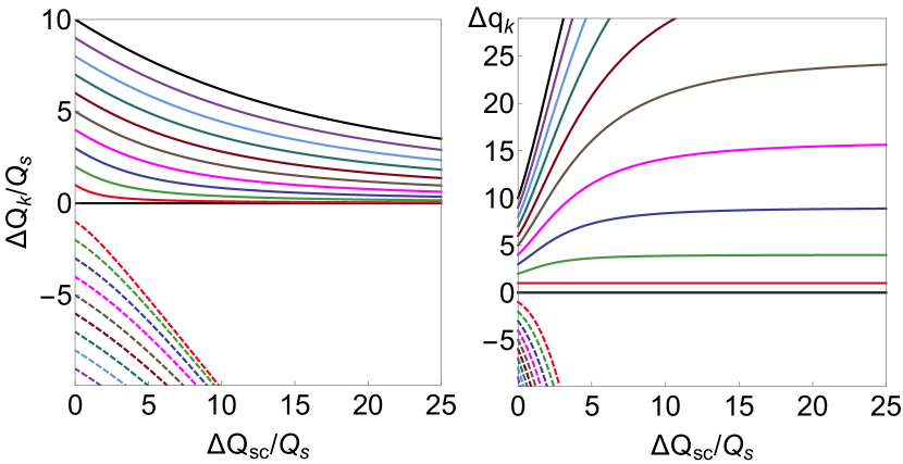
Figure 2: Eigenvalues (left) and normalized eigenvalues (right) for the ABS model as functions of the SC parameter for no-wake case, $k=-9,\ldots,10$. Positive and negative parts of spectrum are shown with solid and dashed lines respectively.

III Negative wakes

Without wakes, all ABS modes are divided into two groups, with positive and negative tune shifts $\Delta Q_{k}$; at growing SC, the former tend to zero, while the latter tend to the SC tune shift. The addition of wake fields will shift the tunes of the modes. It is convenient to number the mode using the same number to which that mode corresponds without wakes. This mode number definition is unambiguous provided that the given mode never coupled with its neighbors at smaller wake amplitudes, which is sufficient for our purposes. Following that, we distinguish all the modes at any wake between positive and negative modes, or positive or negative parts of the spectrum, which is unambiguous provided that there is no coupling between the positive and negative modes, which is always the case below. The reader should not be confused by the fact that wakes may shift tunes of some positive modes to negative values; we still refer to such modes as positive.

In this section, constant-sign wakes are considered for the ABS, as well as for the SSC problems; as it follows from the Maxwell equations, this sign can only be negative Chao (1993). We limit ourselves here by delta-functional, constant, step-function, exponential and resistive wall wakes. All the wakes are assumed to be causal. Sometimes, the tunes at a given wake and SC are convenient to present in units of the first eigenvalue at the same SC and zero wake. To facilitate this, we define

$$\kappa^{*}=\kappa\Big{/}\left[-\frac{\Delta Q_{\mathrm{sc}}}{2\,Q_{\text{s}}}+\ \sqrt{\left(\frac{\Delta Q_{\mathrm{sc}}}{2\,Q_{\text{s}}}\right)^{2}+1}\right].$$ (54)

In these units, the positive part of the spectrum shows scale invariance for large values of $\Delta Q_{\mathrm{sc}}$, Eq. (51). In order to describe the instability, we introduce a dimensionless wake parameter $\chi$ and its normalized value $\chi^{*}$:

$$\chi=\frac{\kappa\,W_{0}}{Q_{\text{s}}}\qquad\text{and}\qquad\chi^{*}=\frac{\kappa^{*}\,W_{0}}{Q_{\text{s}}},$$ (55)

where $\tau_{\mathrm{b}}$ and $W_{0}$ are the bunch length and the wake amplitude specified for every case separately ($\tau_{\mathrm{b}}=3\sigma_{\mathrm{b}}$ for SSCG). When the SC is getting strong, Eq. (55) corresponds to Eq. (12) with $Q_{\text{eff}}(0)/Q_{\text{s}}^{2}$ being understood as units of coherent tune shifts.

III.1 Delta wake

Our first negative-wake example is one of image charges, the delta wake,

$$W(\tau)=-W_{0}\tau_{\mathrm{b}}\,\delta(\tau).$$ (56)

In this case the airbag model allows analytical solution Boine-Frankenheim and Kornilov (2009)

$$\frac{\Delta Q_{k}}{Q_{\text{s}}}=-\frac{\Delta Q_{\mathrm{sc}}+\kappa\,W_{0}}{2\,Q_{\text{s}}}\pm\ \sqrt{\left(\frac{\Delta Q_{\mathrm{sc}}-\kappa\,W_{0}}{2\,Q_{\text{s}}}\right)^{2}+k^{2}},$$ (57)

for $k=\pm 1,\pm 2,\ldots$ and the zeroth mode

$$\Delta Q_{0}/Q_{\text{s}}=-\kappa\,W_{0}.$$

The system is stable for any values of wake amplitude and SC. The first row of Fig. 3 shows normalized tune shift for ABS model as a function of the wake parameter for different values of SC. As the SC parameter is increased, the positive and the negative parts of the spectrum begin to separate, and, at very high SC parameter the bunch spectra corresponds to the one of SSCSW (last plot in the first row of Fig. 3).

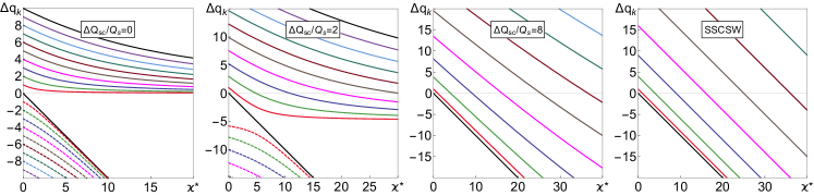
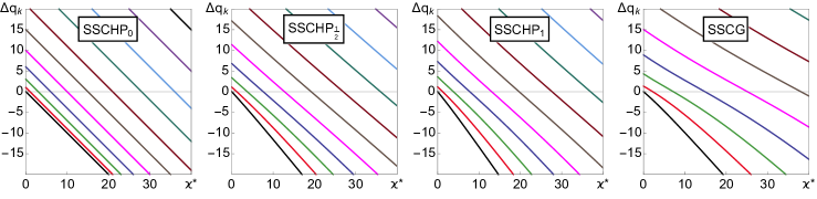
Figure 3: Top row: normalized tune shifts for the ABS model and delta wake for different values of the SC parameter; the last plot in a row is the spectrum at the SSC limit — SSCSW. Bottom row: normalized spectra for remaining SSC models.

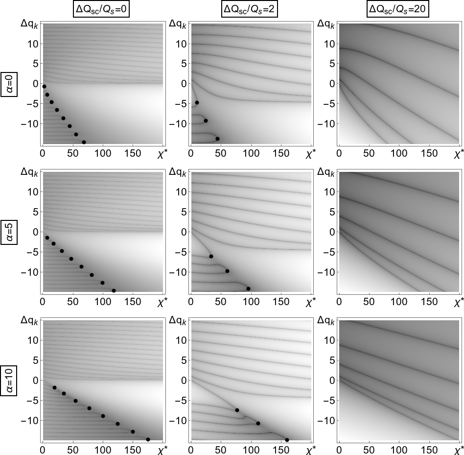
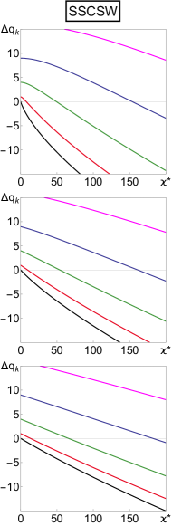
Figure 4: Spectra for the ABS model and constant ($\alpha=0$) or exponential ($\alpha=5,10$) wakes. Different columns correspond to different values of the space charge parameter $\Delta Q_{\mathrm{sc}}/Q_{\text{s}}=0,2,20$. The TMCI thresholds are shown by black points. The last plot in each row is the spectrum at the SSC limit — SSCSW model.

For the SSC models, matrix elements are given by

$$\widehat{\mathrm{W}}_{lm}=-W_{0}\,\int_{\text{SB}}\rho^{2}(\tau)\,Y_{l}(\tau)\,Y_{m}(\tau)\,\mathrm{d}\tau,$$ (58)

and were found numerically for the SSCHP_1/2,1 and SSCG cases. In the case of SSCSW and SSCHP₀ (and any other distribution with constant line density), this integral reduces to

$$\widehat{\mathrm{W}}_{lm}=-W_{0}\,\delta_{lm},$$ (59)

yielding the eigenvalues

$$\Delta q_{k}=\nu_{k}+\kappa\,\widehat{\text{W}}_{kk}=\nu_{k}-\kappa\,W_{0}.$$ (60)

The second row of Fig. 3 shows the normalized tune shift as a function of wake amplitude for all SSCHP and SSCG models. The spectra for the more realistic distributions (SSCHP_1/2,1 and SSCG) are similar to that of SSCHP₀ and SSCSW with the only difference of faster deflection of the zeroth mode compared to the other modes.

The Hamiltonian nature of the system ensures beam stability for delta wakes: the delta wake can be taken into account with a term proportional to a double sum

$$\Sigma_{lm}x_{l}x_{m}\delta(\tau_{l}-\tau_{m})$$

in the total Hamiltonian, where $x_{l}$ and $x_{m}$ are offsets of individual particles and $\tau_{l}$, $\tau_{m}$ are their positions inside the bunch.

III.2 Exponential and constant wakes

As the next example, consider exponential wakes

$$W(\tau)=-W_{0}\,e^{\alpha\,\tau},$$ (61)

including a constant wake, $\alpha=0$. With these wakes, TMCI problem for the ABS model was formulated and solved by M. Blaskiewicz and for HP₀ and SW cases by V. Balbekov, within the SSC approximation Balbekov (2016b, a, 2017a). Here we summarize some of these results and make a comparison with more realistic model of a Gaussian bunch and SSCHP_1/2,1.

III.2.1 ABS model

Figure 4 shows the normalized coherent tune shifts for constant and exponential ($\alpha=5,10$) wakes for the ABS model. As one can see, TMCI may occur only at the negative part of the spectrum and the thresholds monotonically increase with $\Delta Q_{\mathrm{sc}}$. The last two plots in each row show the spectra for large value of SC ($\Delta Q_{\mathrm{sc}}/Q_{\text{s}}=20$) and the one produced from the SSCSW model respectively. These plots look identical to each other and hence show the scale invariance at the SSC limit. Behavior of the TMCI thresholds for these cases is summarized in Fig. 5 which we reproduce, albeit by another method, after M. Blaskiewicz Blaskiewicz (1998). When the instability threshold increases with SC without limit, the TMCI is referred in this paper as vanishing.

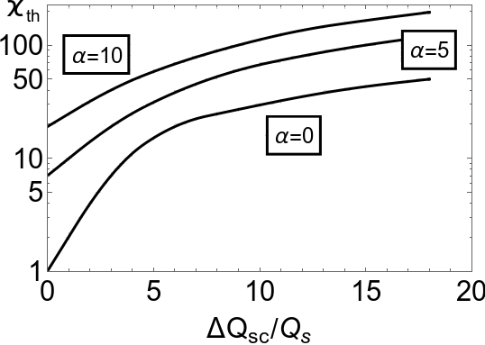
Figure 5: TMCI threshold as a function of SC for the ABS model with the exponential wakes (reproduction of Ref. Blaskiewicz (1998)).

Increase of the TMCI thresholds with space charge was first demonstrated in Ref. Blaskiewicz (1998), soon after that was explained in Ref. Ng and Burov (1999): while the wake deflects down mostly the zeroth mode, and to a lesser extent does that for the mode $\Delta Q_{-1}$, the space charge does exactly the opposite, deflecting down the mode $\Delta Q_{-1}$ and keeping the tune of the mode $0$ untouched; thus, the mode crossing either happens at higher wakes, or does not happen at all. However, it was later speculated in Ref. Burov (2009) that the increase of the threshold with the space charge may be non-monotonic, that at sufficiently high SC tune shift, the TMCI threshold may start to go down. A reason for that speculation was derived from the unlimited reduction of the mode separation with the space charge; when the neighbor modes are closer and closer, it should take less and less to couple them. This speculation was apparently confirmed within the SSC approximation by computation of the TMCI threshold versus the SC tune shift with constant and resistive-wall wakes, where the non-monotonic behavior of the instability threshold was observed. However, those computations of Ref. Burov (2009) were made with an insufficient number of modes and with limited accuracy of the matrix element computation, so the formulated hypothesis remained open. Some supporting results for that were provided by tracking simulations of Ref. Blaskiewicz (2012). This problem was recently addressed by V. Balbekov Balbekov (2017a). Specifically, it has been shown by him, that the TMCI threshold computed for the exponential wakes increases without limit as more basis functions are taken into account. In other words, for such wakes at SSC case there is no TMCI at all, the instability may happen only with comparable SC and wake-driven tune shifts, as in Fig. 5. Below we confirm that with our results.

III.2.2 Convergence of SSC models

In this subsection, we will discuss the question of spectra convergence for SSC models with respect to the number of modes taken into analysis. We will use the constant wake model for illustrative purposes. Figure 6 shows the spectra for SSCSW and SSCHP₀ for constant wake with different number of modes taken into account. Solid lines show real and imaginary parts of the spectra with truncation at 5 harmonics. Dashed lines are the same spectra computed with 50 basis harmonics. Although both cases look similar for smaller values of the wake parameter $\chi^{*}$, we clearly see the onset of instability with 5 harmonics, while no instability is observed when number of harmonics is sufficiently large.

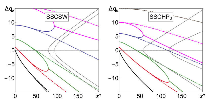
Figure 6: Real (shown in color) and imaginary (gray colors) parts of the spectra for SSCSW and SSCHP₀ with a constant wake. Solid and dashed lines are obtained using 5 or 50 modes respectively. For sufficiently large number of modes and sufficiently good accuracy of the matrix element computations, TMCI vanishes.

Figure 7 summarizes the results stated above. It demonstrates the growth of TMCI threshold with the truncation parameter, a number of harmonics included in the computations. For all the cases, the thresholds monotonically increase with the mode truncation parameter, thus demonstrating that the beam is stable against TMCI. The spectra for all SSCHP and SSCG models subjected to constant and exponential wakes with the same wake decay rates are presented in the Appendix C for the reader to consult; qualitatively, they are similar to the spectra presented in Fig. 6.

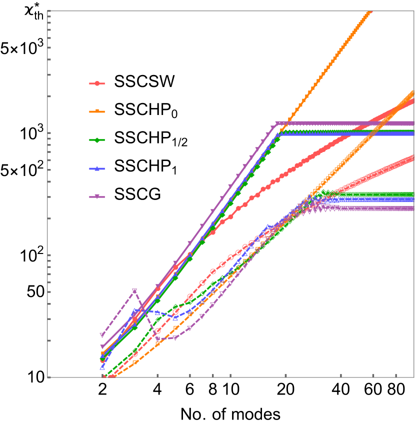
Figure 7: TMCI threshold as a function of number of modes for constant and resistive wall wakes (solid and dashed lines respectively) at SSC. The unlimited growth with the truncation parameter means that there is no TMCI. The saturation of the threshold for numerical models (SSCHP_1/2,1 and SSCG) does not reflect the instability and is due to limited precision of calculated matrix elements, $\widehat{\mathrm{W}}_{lm}$.

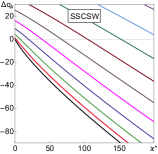
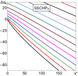
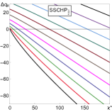
Figure 8: Spectra for SSC models with resistive wall wake, truncated at 40 modes. No TMCI.

III.3 Resistive wall wake

The SSC models can also be considered with the resistive wall wake function

$$W(\tau)=-W_{0}/\sqrt{|\tau|}.$$ (62)

Similar to the exponential and constant wakes, the apparent threshold increases without limit as more modes are taken into account, as it can be seen in Fig. 7; spectra are shown above in Fig 8.

III.4 Step Wake

When the wake is shorter than the bunch length, sometimes it is convenient to approximate it by a step function

$$W(\tau)=W_{0}\left(\text{H}\,[-\tau-\tau_{\text{w}}]-\text{H}\,[-\tau]\right),$$ (63)

where $\tau_{\text{w}}\in(0,1)$ is a characteristic wake length. While this wake was studied with SW and HP₀ models by V. Balbekov, we extend the result for Gaussian bunch and SSCHP_1/2,1 cases. It was established that, for any value of $\tau_{\text{w}}$, TMCI vanishes for all SSC models. The examples of spectra for $\tau_{\text{w}}=0.2,0.4,0.6$ and $0.8$ have been included in the Appendix C.

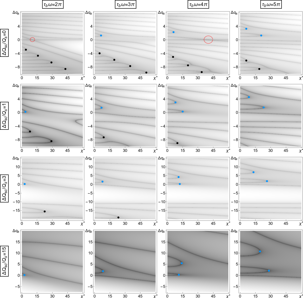
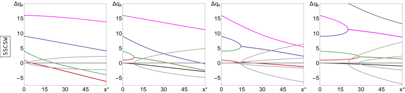
Figure 9: Bunch spectra for the ABS model with cosine wake. The top four rows correspond to various values of SC parameter (0, 1, 3, 15). The vanishing TMCI thresholds are shown with black points and non-vanishing with blue. The red dashed circles indicate mode crossing, when modes do not couple. The last row is for the SSC limit — SSCSW model; the real and imaginary parts of $\Delta q_{k}$ are shown in colors and in gray respectively. The columns correspond to different values of $\omega\,\tau_{\mathrm{b}}$: $2\,\pi$, $3\,\pi$, $4\,\pi$ and $5\,\pi$ from the left to the right respectively.

IV Oscillating wakes

As shown above, the instability for negative wakes takes place only when wake and space charge tune shifts are comparable, i.e. the TMCI is of the vanishing type. At positive (non-physical) wakes, the instability threshold monotonically decreases with the space charge; the wake moves 0-th tune up, while the space charge deflects the tune of the above 1-st mode down, so SC helps the two modes to meet each other. Since the positive wakes are impossible Chao (1993), they are not discussed any more in our paper. What is possible, though, is a combination of positive and negative wakes, i.e. oscillatory wakes. It can be expected that, at least for some of them, the instability threshold decreases with the SC, similar to the positive wakes. In fact, this was already shown for the cosine wake in Ref. Burov (2009): in contrast with negative wakes, the downward deflection of the cosine wake acting on one mode may be more than the deflection of the lower neighboring mode causing mode crossing and possible coupling. Since SC reduces the mode separation, in this case, the instability threshold goes down with an increase of the SC tune shift.

In this section, we consider oscillating wakes of two types: cosine and sine with variable decay rates. All of them can be treated within the ABS model, as suggested in Ref. Blaskiewicz (1998). For comparison, results of the complimentary SSC approximation are also provided below.

IV.1 Cosine wake

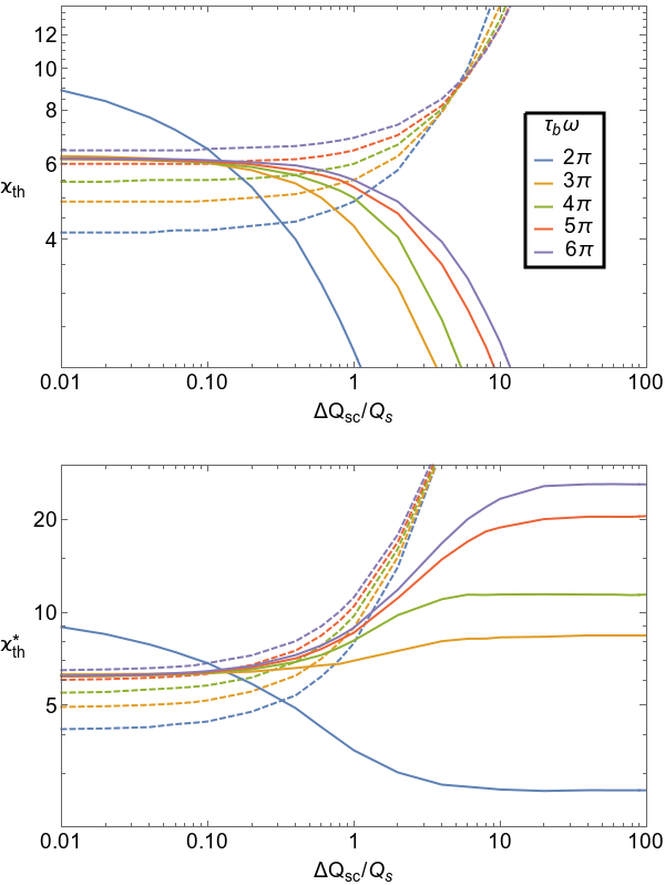
Figure 10: TMCI threshold as a function of space charge for the ABS model and a cosine wake. The dashed and solid lines correspond to the vanishing and non-vanishing TMCIs. The top figure shows thresholds in regular units. The bottom figure shows the same in terms of the normalized wake parameter.

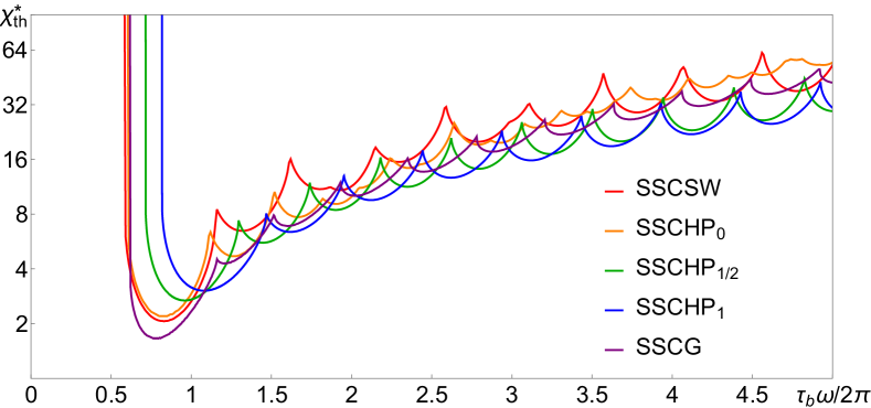
Figure 11: TMCI threshold for all SSC models with cosine wake as a function of wake phase advance $\omega\,\tau_{\mathrm{b}}$. The vertical lines reflect an absolute threshold with respect to $\omega\,\tau_{\mathrm{b}}$.

IV.1.1 ABS Model

For cosine wakes

$$W(\tau)=-W_{0}\cos(\omega\,\tau),$$ (64)

the normalized spectra for different values of the SC tune shift and the wake phase advance $\omega\,\tau_{\mathrm{b}}$ are shown in Fig. 9. When the oscillations are sufficiently pronounced ($\omega\,\tau_{\mathrm{b}}\gtrapprox\pi$), the spectra show that the situation is more diverse here than for the negative wakes: in addition to instabilities in the negative part of the spectra (indicated with black points again), there is a mode coupling for positive modes (blue points). Figure 10 summarizes the behavior of the lowest mode coupling thresholds for the modes with negative and positive indexes. While the TMCIs in the negative part of the spectra vanish, as in the case of constant-sign wakes, TMCI thresholds for positive modes are going down, as was speculated in Ref. Burov (2009); as a result, the TMCI threshold is non-monotonic. On the bottom plot, which repeats the top one in normalized units, one can see the saturated TMCI threshold at high SC, which reflects its inverse proportionality to the SC parameter.

IV.1.2 SSC Limit

In order to summarize the behavior of TMCI in the SSC limit when the bunch is subjected to cosine wake, we considered the threshold as a function of $\omega\,\tau_{\mathrm{b}}$ for all models, see Fig. 11. For smaller values of the wake phase advance, the wake is effectively negative, yielding TMCI has a threshold with respect to $\omega\,\tau_{\mathrm{b}}\approx\pi$, with $\tau_{\mathrm{b}}=3\,\sigma_{\mathrm{b}}$ for SSCG.

At high SC parameter values, all the models give similar results, with the SSCSW model becoming similar to the ABS (compare the 4-th and 5-th rows in Fig. 9). Since the behavior in SSC limit is similar for all cases, the corresponding spectra for all SSCHP and SSCG models have been included in the Fig 22 of Appendix C.

IV.1.3 Convergence in SSC approximation

In contrast to the case of negative wakes, the computed threshold quickly converges with the number of modes taken into account. Examples of convergence of $\chi^{*}_{\text{th}}$ for wake phase advance $\omega\,\tau_{\mathrm{b}}=2\,\pi$ and $3\,\pi$ are presented in Fig. 12. When the number of modes becomes too large (which is about 30 in our case), the SSCHP₀ shows a purely numerical instability: the threshold computations become unstable and its erroneously computed value drops to 0.

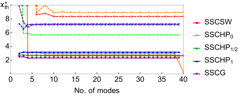
Figure 12: Instability threshold as a function of the number of modes taken into account at the SSC for the cosine wake. Solid and dashed lines correspond to different values of wake phase advance, $\omega\,\tau_{\mathrm{b}}$: $2\,\pi$ and $3\,\pi$ respectively.

IV.2 Sine wake

The sine wake

$$W(\tau)=W_{0}\,\sin(\omega\,\tau),$$ (65)

is considered for the same models as for the cosine wake and the resulting spectra are shown in Figs. 13 and 14.

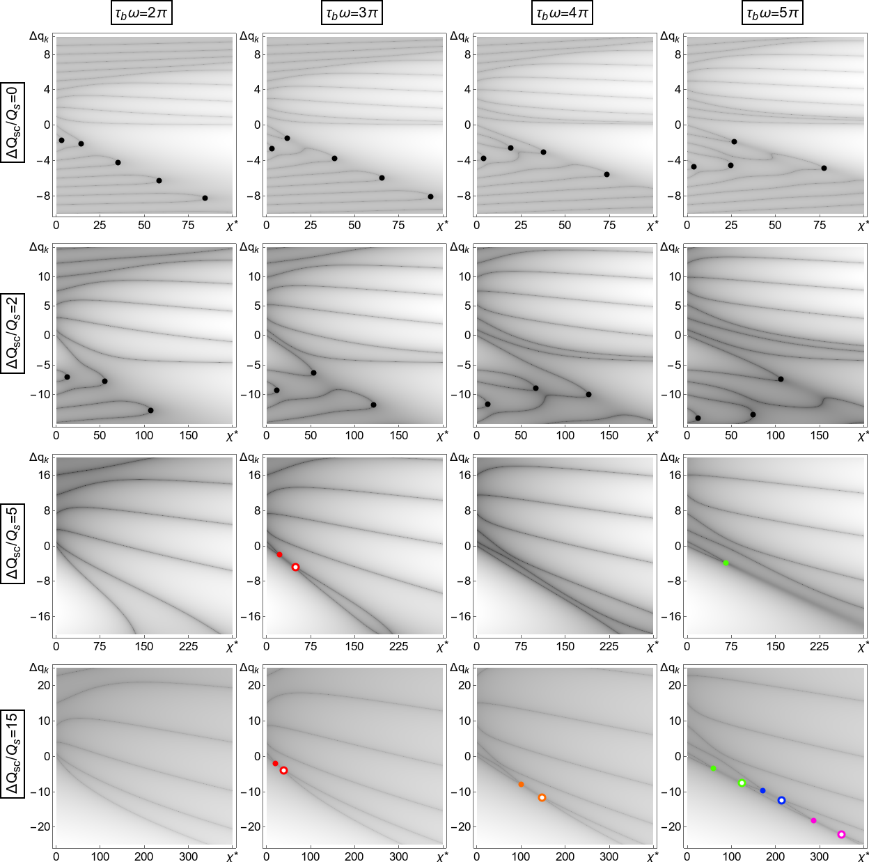
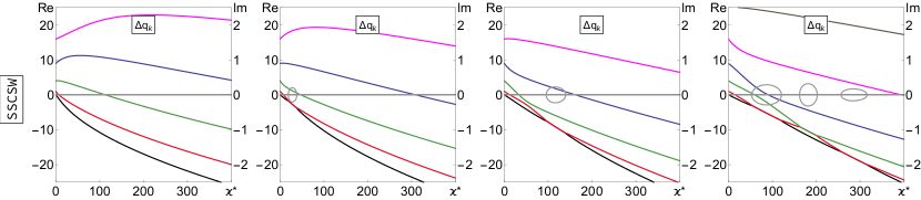
Figure 13: Bunch spectra for the sine wake. The top 4 rows show the ABS spectra for various values of SC (0, 2, 5, 15). The vanishing TMCI thresholds are shown with black and non-vanishing using points in colors (subsequent decoupling for each TMCI is shown by the point of the same color with an annulus). The last row is for the SSCSW model; the real and imaginary parts of $\Delta q_{k}$ are shown in colors and in gray respectively (note the different scaling for real and imaginary parts). The columns correspond to the different values of $\omega\,\tau_{\mathrm{b}}$ ($2\,\pi,3\,\pi,4\,\pi,5\,\pi$).

Figure 14: Bunch spectra for the sine wake with all SSC models. The real and imaginary parts of $\Delta q_{k}$ are shown in colors and in gray respectively (the scaling for the real and imaginary parts is the same as in Fig. 13). The columns correspond to the different values of $\omega\,\tau_{\mathrm{b}}$ ($2\,\pi,3\,\pi,4\,\pi,5\,\pi$). The instability is observed only for SSCSW model. SSCHP₀ spectra show mode crossing without coupling.

Figure 15: TMCI threshold in terms of the usual (top) and normalized (bottom) wake parameters versus the SC parameter for the ABS model and sine wake. The dashed lines correspond to the vanishing TMCI in a negative part of the spectra. The solid and dotted lines represent first couplings and first decouplings for positive modes.

IV.2.1 ABS Model

In the ABS model, the behavior of the negative modes looks similar to the cases of the cosine and negative wakes. In contrast, for the positive modes, there is no instability when the SC is zero, independently of the wake phase advance $\omega\tau_{\mathrm{b}}$ (first row in Fig. 13). However, when the SC is increased, a cascade of mode couplings and decouplings appears (3rd and 4th rows in Fig. 13). When $\omega\,\tau_{\mathrm{b}}=2\,\pi$, the threshold increases with the SC parameter, disappearing at the SSC case. The cases of $\omega\,\tau_{\mathrm{b}}=3\,\pi,4\,\pi$ show a single mode coupling followed by decoupling; the case $\omega\,\tau_{\mathrm{b}}=5\,\pi$ has a cascade of three couplings with subsequent decouplings. For wakes with even more oscillations per bunch, more complicated coupling-decoupling cascades were observed (not shown in the figure). Similar to the cosine wake, Fig. 15 summarizes the behavior of the lowest TMCI thresholds for both negative and positive modes. While all instabilities in the positive part of the spectrum decouple at higher wake parameter, the values of these coupling and decoupling intensities decrease inversely proportional to the SC parameter.

Figure 16: TMCI threshold for SSCSW model with resonator wake as a function of wake phase advance $\omega\,\tau_{\mathrm{b}}$. The different curves correspond to the different values of the wake decay rate, $\alpha\,\tau_{\mathrm{b}}$. The blue curve with $\alpha\,\tau_{\mathrm{b}}=0$ is for the sine wake. The vertical lines reflect an absolute threshold with respect to $\omega\,\tau_{\mathrm{b}}$.

IV.2.2 SSC limit

Figure 14 shows the spectra for all SSC models. The first row is the spectra for SSCSW which are in agreement with the ABS ones when the SC parameter is high enough (as expected). The spectra for SSCHP₀ is shown in the second row. Although it may look similar to both ABS and SSCSW models, they are different because the SSCHP₀ modes never couple. Instead, they either simply cross or approach-divert with respect to each other without coupling. It looks like there is an unknown reason forbidding the instability, and not only for this case.

Indeed, for more realistic distributions, i.e. the SSCHP_1/2,1 and SSCG, there are no instabilities as well (last three rows in Fig. 14). For these cases, the modes never cross each other. Thus, we conclude that there is no TMCI for these more realistic bunch distributions subjected to a sine wake.

The behavior of the non-vanishing TMCI as a function of $\omega\,\tau_{\mathrm{b}}$ for SSCSW is shown in Fig. 16. Similar to the cosine wake, the instability is impossible when the oscillations are not sufficiently pronounced, $\omega\,\tau_{\mathrm{b}}\lessapprox 3\,\pi$. Otherwise the instability threshold is a non-monotonic function of the wake phase advance $\omega\,\tau_{\mathrm{b}}$.

IV.3 Resonator wake

Finally, we consider the spectrum for a decaying sine wake:

$$W=W_{0}\,\sin(\omega\,\tau)\,e^{\alpha\,\tau};$$ (66)

conventionally, this wake function is referred as resonator.

The result for the SSCSW model is shown in Fig. 16. There is no surprise that the instability threshold increases with $\alpha$ for fixed $\omega$. When a certain threshold with respect to the decay parameter $\alpha$ is reached, the instability vanishes: strong enough suppression of the oscillating part by the exponential decay makes the wake effectively negative. Thus, the TMCI vanishes in certain zones of the wake decay and oscillation parameters $\alpha\tau_{\mathrm{b}}$ and $\omega\tau_{\mathrm{b}}$.

The ABS model confirms this result: for fixed $\omega$, when a threshold with respect to $\alpha$ is reached, instabilities in the positive part of the spectrum do not appear, even for large values of space charge. The only instabilities are for the negative modes, vanishing with an increment of SC, as expected. A particular example for CERN SPS ring is discussed in next Subsection IV.4.

In the SSCG and all SSCHP models there is no instability as was in the case of the sine wake; the mode crossing observed in the situation of the SSCHP₀ case turns into an approach-divert behavior and the modes separate when $\alpha$ is increased.

As an example, we compare the SSC theory results with macroparticle simulations of Ref. Blaskiewicz (2012). Two different bunch distributions, HP₀ and HP_7/2, were studied with constant and two resonator wake potentials:

$$\begin{array}[]{l}W_{1}(\tau)=W_{0}\,\sin(12\,\tau)\,e^{1.2\,\tau},\\[5.69046pt] W_{2}(\tau)=W_{0}\,\sin(24\,\tau)\,e^{2.4\,\tau},\end{array}$$

with $\tau$ in units of $\tau_{\mathrm{b}}$. According to Fig. 3 from Blaskiewicz (2012), the dependence of the threshold wake strength as a function of the space charge tune shift is a non-monotonic function. For some cases (HP_7/2 with constant and both HP_0,7/2 with $W_{1}$), the SC stabilizes the beam for $\Delta Q_{\mathrm{sc}}\lessapprox 2\,Q_{\text{s}}$, but then thresholds are getting smaller than without SC, when the last one is increased. For HP₀ with constant wake, the simulations demonstrated stabilization of TMCI with SC with a sign of turning over at larger values of SC. Finally, for HP_7/2 with $W_{2}$ wake, the TMCI threshold monotonically decreases, showing no improvement with SC.

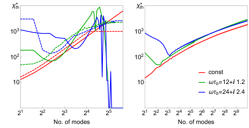
Figure 17: TMCI threshold as a function of the number of modes taken into account for SSCHP₀ (solid lines) and SSCHP_7/2 (dashed lines) models with wake functions from Blaskiewicz (2012). The saturation with number of modes for SSCHP_7/2 case is determined by precision in calculation of matrix elements. For SSCHP₀ with resonator wakes there is the numerical instability of threshold when the number of modes $\approx 20$. Right plot is for SSCHP₀ with the same wakes but using expansion in SSCSW basis: no saturation nor numerical instability is observed.

The macroparticle simulations of Blaskiewicz (2012) can be compared with SSC results shown in Fig. 17. The left figure illustrates the instability threshold as a function of the number of modes taken into account for a boxcar SSCHP₀ and smooth SSCHP_7/2 models with the same wake potentials. Few features of this figure can be noted. First, for both distributions, the calculated threshold goes down with the number of modes until the most resonant mode is added into analysis. Second, numerical effects for the two distributions are different: for the smooth SSCHP_7/2 one can see the saturation with the number of modes, while for the boxcar SSCHP₀ the threshold suddenly drops down after the monotonic growth. In the smooth case, the wake matrix elements were computed using numerical integration and one should not expect the correct result when $\epsilon\,\chi^{*}\approx 1$, which is about the distance between two closest eigenvalues of $\nu_{lm}$, and, $\epsilon$ is the average numerical error for the element of $\widehat{\mathrm{W}}_{lm}$. In the boxcar case, the matrix elements are given by the analytical expressions containing multiple summations (see Appendix A.1 for details). The available algorithm evaluating these sums is numerically unstable for a sufficiently large number $l+m$; as a result, the threshold erroneously tends to zero.

The last effect can be suppressed by using the decomposition of the SSCHP₀ modes using SSCSW basis. Looking for the solution of the Eq. (6) in the form

$$\mathcal{Y}_{k}^{\text{HP}_{0}}(\tau)=\sum_{i=0}^{\infty}\mathbf{B}^{(k)}_{i}Y_{i}^{\text{sw}}(\tau)$$ (67)

where SSCSW harmonics (18) are used instead of Legendre polynomials (27), the eigenvalue problem (10) becomes

$$\mathbf{M}\cdot\mathbf{B}^{(k)}=\Delta q_{k}\mathbf{B}^{(k)},\qquad\mathbf{M}_{lm}=\widehat{\Lambda}_{lm}+\kappa\,\widehat{\mathrm{W}}_{lm}^{\text{sw}},$$ (68)

where $\widehat{\mathrm{W}}_{lm}^{\text{sw}}$ is the wake matrix elements computed for SSCSW model, and, $\Lambda_{lm}$ is the matrix of SSCHP₀ harmonics in SSCSW basis

$$\widehat{\Lambda}_{lm}=\left\{\begin{array}[]{ll}\displaystyle-\frac{(-1)^{\frac{3\,l+m}{2}}4\,l^{2}m^{2}}{(l^{2}-m^{2})^{2}},&\text{if }l+m\text{ is even},\,l\neq m\\[9.95863pt] \displaystyle\frac{1-\delta_{l,0}}{4}+\frac{\pi\,l^{2}}{12},&\text{if }l=m\\[9.95863pt] 0,&\text{otherwise}.\end{array}\right.$$

The result for the same wake potentials is shown in the right plot of Fig. 17. The convergence is slower, since we expanding Legendre polynomials using the trigonometric series, but matrix elements become more stable and significantly larger number of modes can be used in verifying the convergence. As one can see, no sign of numerical instability or saturation is present.

Comparing the results of macroparticle simulations with the SSC theory, it should be noticed the methodical advantage of the last, provided it is applicable: there is only one numerical parameter — the number of modes, allowing a reliable convergence check, while in the first case there are many numerical parameters — a number of macroparticles, number of time steps per betatron oscillation, numerical size of delta functions, spacial grid size and the simulation time. Convergence checks with each of them are required, which cannot be an easy task. Since only one of these checks was reported in Blaskiewicz (2012), a poor convergence with its other numerical parameters could be suspected as a reason for the disagreement between Ref. Blaskiewicz (2012) and this paper.

IV.4 CERN SPS

In this last section we will consider the behavior of TMCI for CERN SPS using ABS model, allowing computations for arbitrary SC parameter. The wake field of the ring is modeled as a broadband resonator, Ref. Quatraro and Rumolo (2010),

$$W(\tau)=Z_{t}\,\frac{\omega_{r}^{2}}{\hat{\omega}\,Q_{r}}\,\sin(\hat{\omega}\,\tau)\,e^{\alpha\tau/2},\;\;\tau<0,$$ (69)

with

$$\hat{\omega}=\sqrt{\omega_{r}^{2}-\alpha^{2}},$$ (70)

$$\alpha=\omega_{r}/(2\,Q_{r}),$$ (71)

$\omega_{r}=1.3\times 2\pi$ GHz, $Q_{r}=1$ and $Z_{t}=5$ $\text{M}\Omega/\text{m}$. For this model, the presumably Gaussian bunch with rms length $\sigma_{\mathrm{b}}=30$ cm is substituted by a boxcar ABS bunch with the total length $\tau_{\mathrm{b}}=3\,\sigma_{\mathrm{b}}$.

Figure 18 shows the behavior of the lowest TMCI threshold as a function of space charge. With the provided decay rate, the wake is effectively negative: the only instabilities are in the negative part of spectrum and they all vanish with the growth of the SC parameter. A complementary Fig. 19 shows the spectra for no space charge case (left plot) and negative part of spectra when $\Delta Q_{\mathrm{sc}}/Q_{\text{s}}=20$. The lowest TMCI threshold is associated with coupling of the $(-6)$-th and $(-7)$-th modes, following the resonator frequency $\omega_{r}$. For parameters from Quatraro and Rumolo (2010), the threshold number of particles at zero SC is $N_{\text{b}}^{\text{th}}=1.8\times 10^{11}$.

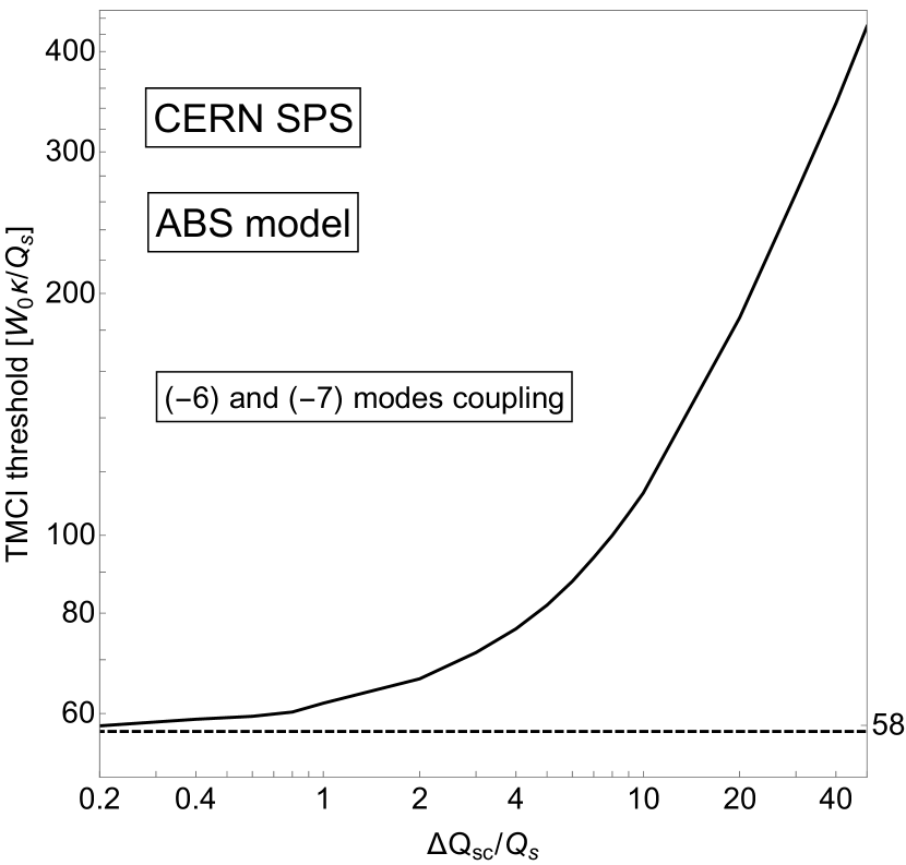
Figure 18: The lowest TMCI threshold as a function of space charge for CERN SPS ring (ABS model). Dashed line shows the value of threshold at zero $\Delta Q_{\mathrm{sc}}$.

This result apparently contradicts Quatraro and Rumolo (2010), where the threshold at high value of SC parameter is almost the same as for the no space charge case. In their case, the space charge parameter, computed with the effective value of the space charge tune shift is $\Delta Q_{\mathrm{sc}}/Q_{\text{s}}=23$; (the effective SC tune shift is a half of its maximum). According to the Fig. 18 the ratio of the thresholds with and without SC should be $\approx 3.5$. The last is confirmed by all SSC models: there is no instability for effectively negative broadband wakes.

To have more confidence in the ABS model, in its application to sinusoidal potential wells, we conducted its study for the high frequency broadband impedance and no SC, comparing its TMCI threshold with ones obtained by the NHT Vlasov solver Burov (2014) and pyHEADTAIL tracking simulations of A. Oeftiger Oeftiger (2018). As one may see from our Ref. Burov and Zolkin (2018), there is a remarkably good agreement between all the three approaches in terms of the threshold values, although the numbers of the coupling modes are higher for the ABS model.

As it was pointed out at the beginning of this article, for the vanishing type of TMCI, there is always an absolute threshold of the wake amplitude, such that the beam is stable for any number of particles as soon as the wake is below its absolute threshold value. Results of Fig. 18 allow to compute the absolute threshold for the SPS parameters of Ref. Quatraro and Rumolo (2010), expressing it in terms of the shunt impedance. For transverse normalized rms emittance $\epsilon_{n}=1.5{\mathrm{mm\cdot mrad}}$ accepted at the referred paper, the absolute threshold comes out as $25{\mathrm{M}\Omega/m}$. Thus, at this emittance, the accepted wake amplitude is about 5 times lower than the absolute threshold, and TMCI should not be seen with any number of particles. For higher emittance, the absolute threshold drops inversely proportionally to that.

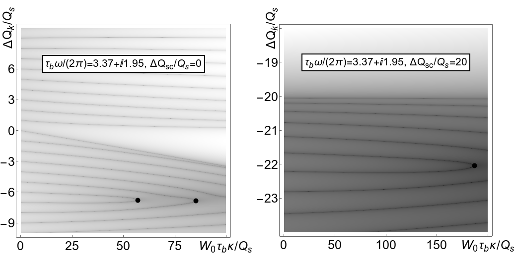
Figure 19: The bunch spectra for the CERN SPS ring in ABS model with broadband resonator wake. The vanishing TMCI thresholds are illustrated with black points. Left plot shows first 20 modes ($k=-10,\ldots,9$) at no SC. Right plot shows only negative part of spectra ($k=-10,\ldots,-1$) at $\Delta Q_{\mathrm{sc}}/Q_{\text{s}}=20$; no TMCI for positive modes. In both cases the lowest TMCI threshold is due to coupling of the $(-6)$-th and $(-7)$-th modes.

A resolution of the contradictions between the observations and macroparticle simulations for the SPS, on the one hand, and the Vlasov analysis of this and preceding publications, on the other, was recently suggested by one of the authors Burov (2018). As shown there, while SC moves up the TMCI wake threshold, it drives the saturating convective instability (SCI) and possibly the absolute-convective instability (ACI), pretty much for the same wake parameters, if not even lower. As a result, the observed wake instability threshold can hardly be considerably larger than its no-SC value.

V Summary

We investigated transverse mode coupling thresholds for various space charge, wakes, potential wells and bunch distribution functions. Two analytical approaches were used, the air-bag square well (ABS) model  Blaskiewicz (1998) and the strong space charge (SSC) theory  Burov (2009, 2015); Balbekov (2009). These approaches are complementary. The former is valid for a specific bunch configuration, allowing an arbitrary space charge, while the latter can be applied for any shape of the potential well and bunch distribution function, provided that SC is sufficiently strong.

As it was explained in Section II, there can be only two types of TMCI with respect to SC. The first one is vanishing TMCI: the threshold value of the wake tune shift $\kappa W_{0}$ grows linearly with the SC tune shift when the latter is high enough; this sort of instability cannot be seen in the SSC approximation, and that is why we call it vanishing. For the vanishing TMCI, there is an absolute threshold of the wake amplitude, such that the beam is stable for any number of particles, provided that the wake amplitude is below its absolute threshold value. Note that the latter is inversely proportional to the transverse emittance and beta-function.

The only other type of TMCI is the SSC one: in this case the threshold of the wake tune shift is asymptotically inversely proportional to the SC tune shift; in fact, it is proportional to $Q_{s}^{2}/Q_{\text{eff}}(0)$. In our studies of particular examples, vanishing type of TMCI was always observed for negative and effectively negative wakes, which agrees with similar results of M. Blaskiewicz and V. Balbekov. The same sort of TMCI has been found for resonator wakes with arbitrary decay rates, for all HP and Gaussian bunches inside a parabolic potential well.

The alternative type of TMCI, the SSC one, takes place for the cosine wakes without respect to the potential well and bunch distribution; it is also the case for the sine wakes at square potential wells, provided that phase advances of the oscillatory wakes are sufficiently large.

We compared our results with available multiparticle simulations with space charge Blaskiewicz (2012); Quatraro and Rumolo (2010), and some contradictions were found. To convince ourselves of correctness of our results, we inspected the agreement of our two models with each other whenever possible; the numerical convergence was thoroughly examined always. For the same purpose, we solved Cauchy problem for the ABS model for several selected cases. For all of them, the thresholds obtained by the described eigensystem analysis were confirmed. A resolution of the contradiction was recently suggested by one of the authors in Ref. Burov (2018), where he treats the SPS Q26 instability not as TMCI but as a convective one.

Appendix A Matrix elements $\widehat{\mathrm{W}}_{lm}$ for SSC models

A.1 Analytical expressions

Calculation of matrix elements for SSCSW model boils down to standard integrals of two trigonometric and an exponential (or inverse square root for resistive wall wake) functions. They are easy to compute and the reader can find them using almost any symbolic computation program; matrix elements for sine and cosine wake functions should be calculated with care when $\omega\,\tau_{\mathrm{b}}=\pi\,n$ with $n$ being integer due to a resonance condition.

For the SSCHP₀ the matrix elements are not that trivial and we provide $\widehat{\mathrm{W}}_{lm}$ with the corresponding wake function $W(\tau)$ in a Table 3 below.

A.2 $\widehat{\mathrm{W}}_{lm}$ for SSCHP_1/2,1 and SSCG models

The numerical evaluation of the double integral of wake matrix elements

$$\widehat{\mathrm{W}}_{lm}=\int_{-\infty}^{\infty}\int_{\tau}^{\infty}W(\tau-\sigma)\,\rho(\tau)\,\rho(\sigma)\,Y_{l}(\tau)\,Y_{m}(\sigma)\,\mathrm{d}\,\sigma\,\mathrm{d}\,\tau$$

is very expensive in terms of CPU time. The use of bunch dipole moments

$$I_{k}(\zeta)=\int_{-\infty}^{\infty}e^{i\,\zeta\,\tau}\,\rho(\tau)\,Y_{k}(\tau)\,\mathrm{d}\tau$$ (72)

along with the impedance function

$$Z^{\perp}(\zeta)=i\,\int_{-\infty}^{\infty}W(\tau)\,e^{-i\,\zeta\,\tau}\,\mathrm{d}\tau$$ (73)

reduces the original expression to a single integral

$$\widehat{\mathrm{W}}_{lm}=(-1)^{m+1}\,i\,\int_{-\infty}^{\infty}Z^{\perp}(\zeta)\,I_{l}(\zeta)\,I_{m}(\zeta)\,\frac{\mathrm{d}\zeta}{2\,\pi}.$$ (74)

Using this method, we are technically still calculating the double integral, but the integrals are decoupled and the inner integral ($I_{k}$) doesn’t depend on a wake function and have to be found just once.

Appendix B Wakes for ABS model

Matrix $\mathrm{M}$ for exponential, cosine and resonator wakes is provided below in a Table 4.

Table 3: Matrix elements $\widehat{\mathrm{W}}_{lm}$ for SSCHP₀ model with negative (delta function, constant, exponential and resistive wall) and oscillating (trigonometric and resonator) wakes. $\widehat{\mathrm{W}}_{lm}$ for all oscillating wakes is expressed using matrix elements of the exponential one.

$W(\tau),\,\tau\leq 0$	$\widehat{\mathrm{W}}_{lm}$
Negative wakes
$-W_{0}\,\delta(\tau)$	$\displaystyle-W_{0}\,\delta_{l,m}$
$-W_{0}$	$\displaystyle-\frac{W_{0}}{2}\left[\delta_{lm,l-m}-(-1)^{\left\lfloor{l/2}\right\rfloor+\left\lfloor{m/2}\right\rfloor}\frac{\delta_{l,m+1}-\delta_{l,m-1}}{\sqrt{(2\,l+1)(2\,m+1)}}\right]$
$-W_{0}\exp(\alpha\,\tau)$	$\displaystyle-W_{0}\sum_{lm}^{ij}\frac{j!}{\alpha^{j+1}}\sum_{k=0}^{j}2^{j-k+1}\frac{\alpha^{k}}{k!}\left\{\frac{1+(-1)^{i+k}}{i+k+1}-\frac{e^{-\alpha/2}}{(-\alpha/2)^{i+1}}\left[\Gamma(i+1,\alpha/2)-\Gamma(i+1,-\alpha/2)\right]\right\}$
$-W_{0}/\sqrt{|\tau|}$	$\displaystyle-\frac{W_{0}}{\sqrt{2}}\sum_{lm}^{ij}\frac{2^{i+j+\frac{3}{2}}}{i+j+\frac{3}{2}}\,\sum_{k=0}^{j}\frac{(-1)^{i+k}}{j-k+\frac{1}{2}}\,\begin{bmatrix}j\\ k\end{bmatrix}\,_{2}F_{1}\left[-\left(i+j+\frac{3}{2}\right);-\left(i+k\right);-\left(i+j+\frac{1}{2}\right);\frac{1}{2}\right]$
Oscillating wakes
$-W_{0}\cos(\omega\,\tau)$	$\Re\left[\widehat{\mathrm{W}}_{lm}^{\mathrm{exp}}(i\,\omega)\right]$
$W_{0}\sin(\omega\,\tau)$	$-\Im\left[\widehat{\mathrm{W}}_{lm}^{\mathrm{exp}}(i\,\omega)\right]$
$W_{0}\sin(\omega\,\tau)\,\exp(\alpha\,\tau)$	$-\Im\left[\widehat{\mathrm{W}}_{lm}^{\mathrm{exp}}(\alpha+i\,\omega)\right]$

Table 4: Matrix $\mathrm{M}$ for ABS model with exponential (or constant for $\alpha=0$), cosine and resonator (or sine for $\alpha=0$) wake functions.

$W(\tau),\,\tau\leq 0$	$\mathrm{M}$
$-W_{0}\,e^{\alpha\,\tau}$	$\begin{bmatrix}i\,\pi\left(\frac{1}{2}\frac{\Delta Q_{\mathrm{sc}}}{Q_{\text{s}}}+\frac{\Delta Q_{k}}{Q_{\text{s}}}\right)&-i\,\pi\,\frac{1}{2}\frac{\Delta Q_{\mathrm{sc}}}{Q_{\text{s}}}&i\,\pi\\ i\,\pi\,\frac{1}{2}\frac{\Delta Q_{\mathrm{sc}}}{Q_{\text{s}}}&-i\,\pi\left(\frac{1}{2}\frac{\Delta Q_{\mathrm{sc}}}{Q_{\text{s}}}+\frac{\Delta Q_{k}}{Q_{\text{s}}}\right)&-i\,\pi\\ -\frac{1}{2}\frac{\kappa\,W_{0}\tau_{\mathrm{b}}}{Q_{\text{s}}}&-\frac{1}{2}\frac{\kappa\,W_{0}\tau_{\mathrm{b}}}{Q_{\text{s}}}&\alpha\,\tau_{\mathrm{b}}\\ \end{bmatrix}$
$-W_{0}\,\cos(\omega\,\tau)$	$\begin{bmatrix}i\,\pi\left(\frac{1}{2}\frac{\Delta Q_{\mathrm{sc}}}{Q_{\text{s}}}+\frac{\Delta Q_{k}}{Q_{\text{s}}}\right)&-i\,\pi\,\frac{1}{2}\frac{\Delta Q_{\mathrm{sc}}}{Q_{\text{s}}}&i\,\pi&i\,\pi\\ i\,\pi\,\frac{1}{2}\frac{\Delta Q_{\mathrm{sc}}}{Q_{\text{s}}}&-i\,\pi\left(\frac{1}{2}\frac{\Delta Q_{\mathrm{sc}}}{Q_{\text{s}}}+\frac{\Delta Q_{k}}{Q_{\text{s}}}\right)&-i\,\pi&-i\,\pi\\ -\frac{1}{4}\frac{\kappa\,W_{0}\tau_{\mathrm{b}}}{Q_{\text{s}}}&-\frac{1}{4}\frac{\kappa\,W_{0}\tau_{\mathrm{b}}}{Q_{\text{s}}}&i\,\omega\,\tau_{\mathrm{b}}&0\\ -\frac{1}{4}\frac{\kappa\,W_{0}\tau_{\mathrm{b}}}{Q_{\text{s}}}&-\frac{1}{4}\frac{\kappa\,W_{0}\tau_{\mathrm{b}}}{Q_{\text{s}}}&0&-i\,\omega\,\tau_{\mathrm{b}}\end{bmatrix}$
$W_{0}\,\sin(\omega\,\tau)\,e^{\alpha\,\tau}$	$\begin{bmatrix}i\,\pi\left(\frac{1}{2}\frac{\Delta Q_{\mathrm{sc}}}{Q_{\text{s}}}+\frac{\Delta Q_{k}}{Q_{\text{s}}}\right)&-i\,\pi\,\frac{1}{2}\frac{\Delta Q_{\mathrm{sc}}}{Q_{\text{s}}}&i\,\pi&i\,\pi\\ i\,\pi\,\frac{1}{2}\frac{\Delta Q_{\mathrm{sc}}}{Q_{\text{s}}}&-i\,\pi\left(\frac{1}{2}\frac{\Delta Q_{\mathrm{sc}}}{Q_{\text{s}}}+\frac{\Delta Q_{k}}{Q_{\text{s}}}\right)&-i\,\pi&-i\,\pi\\ -\frac{i}{4}\frac{\kappa\,W_{0}\tau_{\mathrm{b}}}{Q_{\text{s}}}&-\frac{i}{4}\frac{\kappa\,W_{0}\tau_{\mathrm{b}}}{Q_{\text{s}}}&(\alpha+i\,\omega)\,\tau_{\mathrm{b}}&0\\ \frac{i}{4}\frac{\kappa\,W_{0}\tau_{\mathrm{b}}}{Q_{\text{s}}}&\frac{i}{4}\frac{\kappa\,W_{0}\tau_{\mathrm{b}}}{Q_{\text{s}}}&0&(\alpha-i\,\omega)\,\tau_{\mathrm{b}}\end{bmatrix}$

Appendix C Additional spectra for SSC models

Complementary SSC bunch spectra for constant and exponential (Fig. 20), step-function (Fig. 21) and cosine (Fig. 22) wakes are provided below.

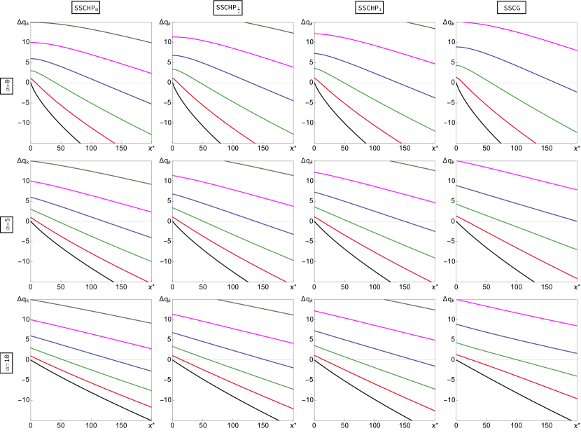
Figure 20: Bunch spectra for SSCHP${}_{0,\frac{1}{2},1}$ (1st – 3rd columns) and SSCG (4th column) models with the constant and exponential wakes. Different rows correspond to the different values of $\alpha=0,5,10$ measured in units of $\tau_{\mathrm{b}}$ with $\tau_{\mathrm{b}}=3\,\sigma_{\mathrm{b}}$ for SSCG.

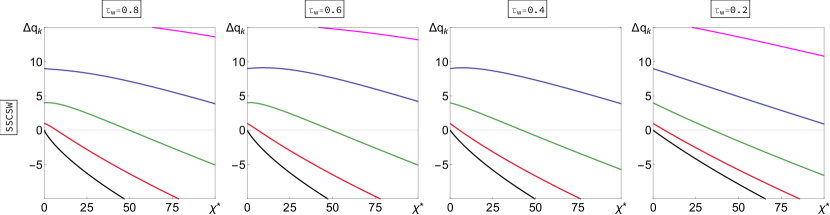
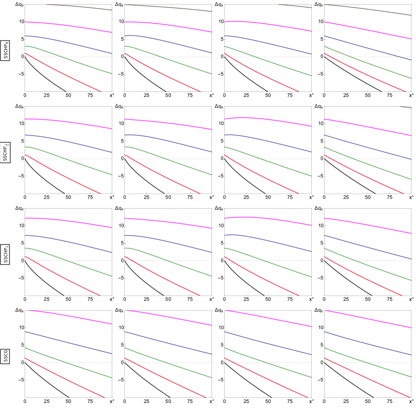
Figure 21: Bunch spectra for all SSC models with the step wake. Different columns correspond to the different values of wake length $\tau_{\text{w}}=0.8,0.6,0.4$ and $0.2$ measured in units of $\tau_{\mathrm{b}}$ (or $3\,\sigma_{\mathrm{b}}$ for SSCG).

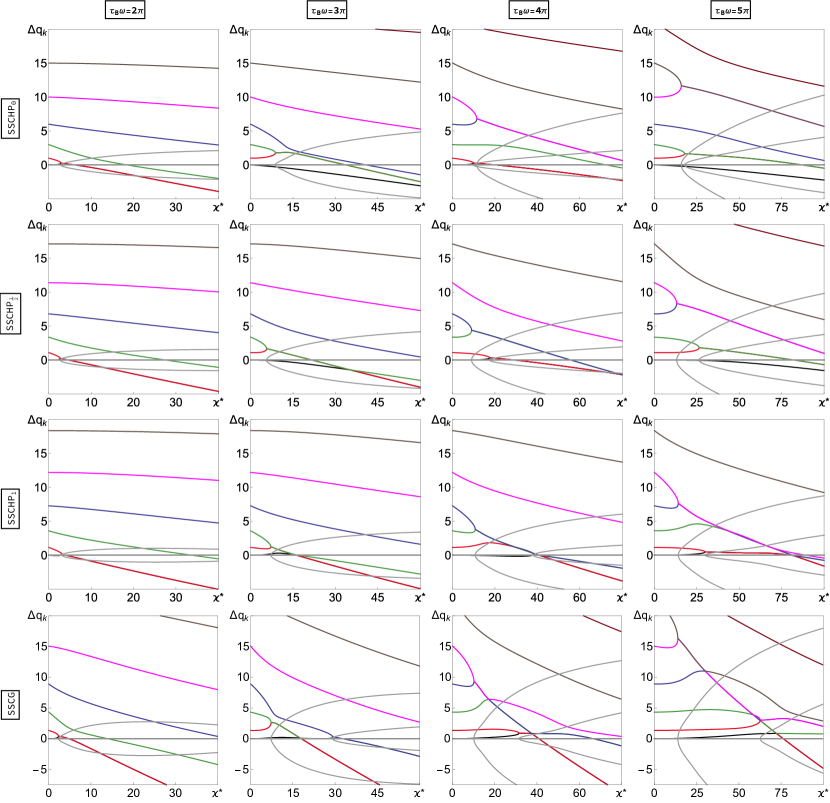
Figure 22: Bunch spectra for SSCHP_0,1/2,1 (1st – 3rd rows) and SSCG (bottom row) models with the cosine wake. Real and imaginary parts of the spectra are shown in colors and gray respectively. The columns correspond to the different values of wake phase advance $\omega\,\tau_{\mathrm{b}}$ with $\tau_{\mathrm{b}}=3\,\sigma_{\mathrm{b}}$ for SSCG.

References

- Chao (1993) A. W. Chao, Physics of collective beam instabilities in high energy accelerators (Wiley, 1993).
- Blaskiewicz (1998) M. Blaskiewicz, Physical Review Special Topics-Accelerators and Beams 1, 044201 (1998).
- Ng and Burov (1999) K. Ng and A. V. Burov, in AIP Conference Proceedings, Vol. 496 (AIP, 1999) pp. 49–63.
- Burov (2009) A. Burov, Physical Review Special Topics-Accelerators and Beams 12, 044202 (2009).
- Balbekov (2009) V. Balbekov, Physical Review Special Topics-Accelerators and Beams 12, 124402 (2009).
- Balbekov (2016a) V. Balbekov, arXiv preprint arXiv:1608.06243 (2016a).
- Balbekov (2016b) V. Balbekov, arXiv preprint arXiv:1607.06076 (2016b).
- Balbekov (2017a) V. Balbekov, Physical Review Accelerators and Beams 20, 034401 (2017a).
- Balbekov (2017b) V. Balbekov, Phys. Rev. Accel. Beams 20, 114401 (2017b).
- Hofmann and Pedersen (1979) A. Hofmann and F. Pedersen, IEEE transactions on nuclear science 26, 3526 (1979).
- Chin et al. (2016) Y. H. Chin, A. W. Chao, and M. M. Blaskiewicz, Physical Review Accelerators and Beams 19, 014201 (2016).
- Blaskiewicz (2012) M. Blaskiewicz, in Conf. Proc., Vol. 1205201 (2012) pp. 3165–3167.
- Quatraro and Rumolo (2010) D. Quatraro and G. Rumolo, Proceedings, 1st International Particle Accelerator Conference (IPAC’10): Kyoto, Japan, May 23-28, 2010, Tech. Rep. (2010).
- Macridin et al. (2015) A. Macridin, A. Burov, E. Stern, J. Amundson, and P. Spentzouris, Phys. Rev. ST Accel. Beams 18, 074401 (2015).
- Boine-Frankenheim and Kornilov (2009) O. Boine-Frankenheim and V. Kornilov, Phys. Rev. ST Accel. Beams 12, 114201 (2009).
- Burov (2014) A. Burov, Phys. Rev. ST Accel. Beams 17, 021007 (2014).
- Oeftiger (2018) A. Oeftiger, “private communication,” (2018).
- Burov and Zolkin (2018) A. Burov and T. Zolkin, arXiv preprint arXiv:1806.07521 (2018).
- Burov (2018) A. Burov, arXiv preprint arXiv:1807.04887 (2018).
- Burov (2015) A. Burov, arXiv preprint arXiv:1505.07704 (2015).