Majorana Zero Modes in Synthetic Dimensions

Abstract

Recent experimental advances in the field of cold atoms led to the development of novel techniques for producing synthetic dimensions and synthetic magnetic fields, thus greatly expanding the utility of cold atomic systems for exploring exotic states of matter. In this paper we investigate the possibility of using experimentally tunable interactions in such systems to mimic the physics of Majorana chains, currently a subject of intense research. Crucially to our proposal, the interactions, which are local in space, appear non-local in the synthetic dimension. We use this fact to induce coupling between counter-propagating edge modes in the quantum Hall regime. For the case of attractive interactions in a system composed of two tunneling-coupled chains, we find a gapless quasi-topological phase with a doubly-degenerate ground state. While the total number of particles in the system is kept fixed, this phase is characterized by strong fluctuations of the pair number in each chain. Each ground state is characterized by the parity of the total particle number in each chain, similar to Majorana wires. However, in our system this degeneracy persists for periodic boundary conditions. For open boundary conditions there is a small splitting of this degeneracy due to the single-particle hopping at the edges. We show how subjecting the system to additional synthetic flux or asymmetric potentials on the two chains can be used to control this nonlocal qubit. We propose experimental probes for testing the nonlocal nature of such a qubit and measuring its state.

I Introduction

Physical systems exhibiting topological order, interesting in their own right, have become a subject of intense attention recently due to their potential utility for quantum information processing Nayak et al. (2008). Much of the recent experimental effort has been focused on one- and quasi-one-dimensional systems hosting Majorana zero modes Alicea (2012); Beenakker (2013), in part due the recent advances in fabricating these systems using semiconducting nanowires, chains of atoms deposited on the surface of a superconductor and other similar systems. Meantime, a steady progress in the field of cold atoms led to the creation a new experimental toolbox Goldman et al. (2016), allowing new avenues for testing similar ideas outside of the realm of condensed matter systems. Interactions between atoms in cold atomic systems can be custom-tailored by coupling individual atomic states to light. At the same time, recent advances led to the dual possibility of creating synthetic gauge fields and endowing these systems with an extra synthetic dimension Celi et al. (2014). Using this approach, two recent milestone experiments demonstrated realizations of quantum Hall-like states and their associated chiral edge modes in synthetic ribbons with artificial gauge fields, one using fermions Mancini et al. (2015) and the other one – bosons Stuhl et al. (2015).

In addition, this approach opens interesting new possibilities for quantum engineering of topological states, e.g. 4D quantum Hall states Price et al. (2015), or for inducing strong correlation effects in low dimensions, e.g. in magnetic crystals Barbarino et al. (2015) where one could observe fractional charge pumping Zeng et al. (2015); Taddia et al. (2017) and probe signatures of chiral Laughlin-like edge states Petrescu and Le Hur (2015); Cornfeld and Sela (2015); Calvanese Strinati et al. (2017); Petrescu et al. (2017).

In this paper, we discuss the possibility of realizing topological states with Majorana-like zero modes within the aforementioned approach which relies on synthetic dimensions/synthetic gauge fields. Specifically, we demonstrate the appearance of such modes in a cold atomic system where a pairing interaction is induced between quantum Hall-like states “separated” in the synthetic dimension. Our proposal builds on an earlier proposal for inducing superconducting proximity in the helical edges of 2D topological insulators Fu and Kane (2008), an influential idea which led to subsequent proposals for Majorana zero modes in semiconductor nanowire settings Lutchyn et al. (2010); Oreg et al. (2010) as well as more recent fractional generalizations Clarke et al. (2013); Lindner et al. (2012); Cheng (2012); Alicea and Fendley (2016). Crucially, our setup is different from the usual condensed matter schemes in that it utilizes a closed system with particle conservation Cheng and Tu (2011); Sau et al. (2011); Kraus et al. (2013); Ruhman et al. (2015); Iemini et al. (2015); Mazza et al. (2015); Chen et al. (2017); Guther et al. (2017).

The idea of additional “synthetic” dimensions is schematically illustrated in Fig. 1, with the role of an extra “dimension” played by an internal atomic degree of freedom, such as nuclear spin. This extra dimension is intrinsically both discrete and finite, nonetheless it allows one to effectively turn a physical 1D atomic chain into a 2D strip/ladder.

A key feature of the synthetic dimension approach is that interactions become non-local in the synthetic dimension Celi et al. (2014); see Fig. 1(a,b). This opens a new possibility, which we exploit in our proposal: namely, it allows coupling between the degrees of freedom which are normally spatially separated in the usual condensed matter setting. In particular, this enables us to create attractive interactions between counter-propagating quantum Hall edge states Yan et al. (2015) in order to induce superconducting instabilities; see Fig. 1(c).

In what follows, we will focus on a system consisting of two identical chains, forming two synthetic ribbons in the quantum Hall regime. Using the renormalization group analysis Cheng and Tu (2011), we show that this closed system forms a many-body phase with strong pair-tunneling coupling between the two chains. Its ground state is doubly degenerate ground state, resembling that of the Kitaev chain Kitaev (2001). However, the total number of particles is fixed in our case. This is the crucial difference between our approach and a related earlier proposal presented in Ref. [Yan et al., 2015] where a single Hall ribbon has been treated in a BCS mean-field approximation. By its nature, such a mean-field approximation breaks particle number conservation, leading the authors of Ref. [Yan et al., 2015] to a physically tenuous conclusion about the existence of Majorana zero modes in their setup. In contrast, our approach does not rely on the mean-field approximation; we show that the prerequisite pairing instability is triggered by arbitrarily weak attractive interactions. Nevertheless, the presence of interactions is crucial here; zero modes found in a related, but non-interacting setup in Ref. [Klinovaja and Loss, 2013] are of the Su–Schriefer–Heeger Su et al. (1980), not Majorana type. (In particular, those zero modes can be individually occupied or empty, implying e.g. the wrong quantum dimension that is inconsistent with the claimed non-Abelian braiding statistics of the Ising type.) Meantime the particle conservation constraint is circumvented in our case by considering a double synthetic ribbon. The ground state degeneracy is no longer associated with the overall fermion parity of the closed system and is instead encoded in the parity in each chain.

The crucial advantage of using the quantum Hall regime is that it naturally allows for generalizations to the fractional case, where we expect that with small modifications the present setup will allow an experimental realization of fractional topological superconductor phases containing exotic anyons, e.g. of the parafermion type. In this paper we shall concentrate on the proof of concept for the simplest possible case, leaving such generalization to fractional state to the future.

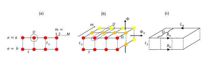
Figure 1: (a) Two coupled chains with an on-site interaction $U$ and internal atomic quantum number $m=1,...,M$. $m$ is conserved upon either intrachain ($t$) or interchain ($t_{\perp}$) hopping. (b) Equivalent picture where quantum number $m$, $1\leq m\leq M$, is interpreted as an additional “dimension”. In addition a finite transition amplitude $m\to m+1$ is included ($\Omega$) with imprinted phase $\Phi$. (c) In the quantum Hall regime the bulk modes $m=1,M$ are gapped and at low energy the system consists of edge modes. Counter propagating edge modes interact non-locally via the initially on-site Hubbard interaction $U$.

II Model

We consider a double chain, or two-leg ladder, of atoms with an internal quantum number $m=1,..,M$, as shown in Fig. 1(a). Atoms can hop along the chain or between the two chains with hopping amplitudes $t$ and $t_{\perp}$ respectively. These hopping processes conserve the internal quantum number $m$. In addition, our model allows internal transitions $m\to m\pm 1$ with amplitude $\Omega$ and an imprinted phase $\Phi$, which can be achieved in practice by illuminating the system by additional lasers at judiciously chosen angles Celi et al. (2014). These transitions can be regarded as hopping in the transverse ‘synthetic’ direction. I.e., each leg of the physical ladder is now effectively a strip, as shown in Figure 1(b). Finally, an on-site interaction $U$ – see in Fig. 1(a) – becomes in effect a non-local interaction within each synthetic strip. The resulting tight binding Hamiltonian for our system is $H_{\text{lattice}}=H_{t}+H_{\perp}+H_{\Omega}+H_{int}$ where

$$H_{t}=-t\sum_{x,\sigma,m}(c^{\dagger}_{x,m,\sigma}c_{x+1,m,\sigma}+h.c.),$$ (1a)

$$H_{\perp}=t_{\perp}\sum_{x,m}\left(e^{i\Phi_{x}\frac{m}{M}}c^{\dagger}_{x,m,a}c_{x,m,b}+h.c.\right),$$ (1b)

$$H_{\Omega}=\Omega\sum\limits_{x,\sigma}\sum\limits_{m=1}^{M-1}\left(e^{ix\Phi}c^{\dagger}_{x,m,\sigma}c_{x,m+1,\sigma}+h.c.\right),$$ (1c)

$$H_{int}=U\sum_{x,\sigma}n_{x,\sigma}^{2}.$$ (1d)

Here, $\sigma=\{a,b\}$ labels the legs (strips) of the ladder, and $n_{x,\sigma}=\sum_{m}c^{\dagger}_{x,m,\sigma}c_{x,m,\sigma}$. The inter-chain tunneling term (1b) also also allows for a position-dependent tunneling phase $\Phi_{x}$, which will be discussed later.

In what follows, we focus on the case of strongly anisotropic tunneling, specifically $t_{\perp}\ll t$. We envision each of the synthetic strips to be in the quantum Hall regime, so that the system forms two weakly coupled quantum Hall strips, which requires the following relation between the model parameters:

$$|U|,t_{\perp}\ll\Omega\ll t.$$ (2)

Let us first consider the case of decoupled strips, $t_{\perp}=0$. A single particle dispersion relation in the absence of the interaction term (1d) is shown in Fig. 2. When there is no tunneling in the synthetic dimension as well ($\Omega=0$), the dispersion relation for each strip ($\sigma=a,b$) consists of $M$ cosines (dashed lines in in Fig. 2), shifted with respect to one another horizontally in the momentum space due to the presence of the synthetic magnetic flux $\Phi$. For finite $\Omega$, $m\to m\pm 1$ transitions lead to avoided crossings and open gaps (solid lines in Fig. 2). Each synthetic strip thus realises a coupled-wire construction of Ref. [Kane et al., 2002]. We assume that the temperature is lower than the quantum Hall gap $\Omega$, allowing one to reach the quantum Hall regime. Specifically we consider the filling factor $\nu=1$, meaning that the Fermi level lies within the first gap, as shown in Fig. 2. This corresponds to the number of atoms per (synthetic) site being $\langle n_{x,m,\sigma}\rangle=\Phi/2\pi$.

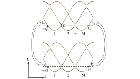
Figure 2: Energy-momentum diagram and interaction processes of the model Eq. (1). The cosine dispersions for each $m$ are shifted in momentum space due to the flux $\Phi$ (dashed lines). The $m\to m\pm 1$ processes $\Omega$ create avoided crossings and open energy gaps separating Landau levels (full lines). Two counter propagating edge modes $R_{\sigma}$, $L_{\sigma}$ remain at the Fermi level (dashed line) for each chain $\sigma=a,b$. Among interaction processes, the pair tunneling term transfers two particles between the two chains. It is facilitated by the non-local interaction $U$ between the edge states.

In the quantum Hall regime all modes in the bulk ($1<m<M$) are gapped and the low energy physics is governed solely by the two chiral edge states crossing the Fermi level. Specifically, for each physical chain of atoms $\sigma=a,b$, the first synthetic chain $m=1$ hosts a left-moving mode, and the $M$-th synthetic chain hosts a right-moving edge mode,

$$c_{x,M,\sigma}=e^{ik_{F}^{\sigma}x}R_{\sigma}(x),~{}~{}~{}c_{x,1,\sigma}=e^{-ik_{F}^{\sigma}x}L_{\sigma}(x).$$ (3)

Here $R_{\sigma}(x)$, $L_{\sigma}(x)$ are slowly varying fermionic fields (we have set the short distance cut-off $a_{0}=1$). The effective edge Hamiltonian is $H_{edge}=\int dx\left(\mathcal{H}_{0}+\mathcal{H}_{\perp}\right)$, where

$$\mathcal{H}_{0} =\sum_{\sigma}\left(iv_{\sigma}\left[R_{\sigma}^{\dagger}\partial_{x}R_{\sigma}-L^{\dagger}_{\sigma}\partial_{x}L_{\sigma}\right]+UR^{\dagger}_{\sigma}R_{\sigma}L^{\dagger}_{\sigma}L_{\sigma}\right)$$ (4a)

$$\mathcal{H}_{\perp} =t_{\perp}\left(e^{-i\delta kx}e^{i\Phi_{x}/2}R^{\dagger}_{a}R_{b}+e^{i\delta kx}e^{-i\Phi_{x}/2}L^{\dagger}_{a}L_{b}\right)+h.c.$$ (4b)

The first term contains both the kinetic energy and density–density interaction within each physical chain. Here $v_{\sigma}=2t\sin(k_{F}^{\sigma})$ where $k_{F}^{\sigma}=n_{\sigma}\pi$ with $n_{\sigma}=\langle\hat{n}_{x,\sigma,m}\rangle$ being the average density in each synthetic chain. We shall ignore band curvature and hence assume $v_{a}=v_{b}=v_{F}$. The second term describes tunneling between the two physical chains; using Eq. (3) we can see that for a finite density difference between the two chains this term oscillates as $e^{i\delta kx}$ where $\delta k=k_{F}^{a}-k_{F}^{b}$ and is therefore irrelevant as long as $k_{F}^{a}\neq k_{F}^{b}$.

III Superconducting phase for attractive interactions

With the goal of realising topological superconducting states, we now turn to the analysis of our model in the case of attractive interactions, $U<0$, which is a realistic possibility in the realm of cold atoms. For our analysis to be self-contained, we shall review some previous results on Majorana fermions in setups with particle number conservation Cheng and Tu (2011); Keselman and Berg (2015); Chen et al. (2017), whose effective description closely matches that of Eq. (4). We will emphasize features and experimental knobs that are specific to our proposed setup based on synthetic quantum Hall ribbons, particularly the role of the non-locality of interactions in the synthetic dimension and the flux $\Phi_{x}$ inserted within a loop in the plane containing the synthetic dimension. We begin by characterizing the resulting superconducting phase from the point of view of a Luttinger liquid instability to pair tunneling, see Fig. 2, by following the analysis and notations of Cheng and Hao Cheng and Tu (2011) who studied an identical effective model. We will address its ground state degeneracy using bosonization. In close analogy to the analysis of Ref. Chen et al., 2017, we will construct Majorana operators and show that the model has an emergent $Z_{2}$ symmetry obtained at a special value of the flux $\Phi_{x}$; when projected to the low energy subspace, this $Z_{2}$ symmetry coincides with the parity symmetry generated by the Majorana operators and hence protects the ground state degeneracy from local perturbations.

III.1 Renormalization group analysis

In the presence of interactions, the inter-chain tunneling [see Eq. (4b)] results in the generation of two more quartic terms in the effective low-energy Hamiltonian: simultaneous backscattering within the two physical chains, and pair tunneling between them. These terms are proportional to $\left(e^{2i\delta kx}L_{a}^{\dagger}R_{a}R_{b}^{\dagger}L_{b}+h.c.\right)$ and $R_{a}^{\dagger}L_{a}^{\dagger}L_{b}R_{b}$ respectively. As can be seen from Fig. 2, at energies much smaller than $\Omega$ these processes involve just the edge modes. Under normal circumstances the amplitudes of these processes would be suppressed due to the spatial separation of the counter-propagating edge modes. However, in our setting this separation occurs in the synthetic dimension, resulting in no such suppression: the interaction $U$ is nonlocal in this dimension.

Notice that for a finite density imbalance between the chains, $\delta k=k_{F}^{a}-k_{F}^{b}\neq 0$, while both the single particle tunneling described by Eq. (4b) as well as the aforementioned simultaneous backscattering operator do not conserve momentum and, as a result, oscillate with wavenumbers $\delta k$ and $2\delta k$ respectively. Meantime, the induced pair tunneling term does not oscillate. This property can be used to selectively promote the pair tunneling process.

It is convenient to bosonize this model,

$$R(L)_{\sigma}=\frac{1}{\sqrt{2\pi a_{0}}}e^{i\sqrt{\pi}(\theta_{\sigma}+r\varphi_{\sigma})},$$ (5)

where $r=+/-$ for $R/L$ and $\sigma=a,b$; $a_{0}$ is a short distance cutoff, and the two bosonic fields satisfy $[\partial_{x}\varphi_{\sigma}(x),\theta_{\sigma}(x^{\prime})]=i\delta(x-x^{\prime})$. The field $\varphi_{\sigma}$ is related to the charge density in chain $\sigma$ via $\rho_{\sigma}=\frac{1}{\sqrt{\pi}}\partial_{x}\varphi_{\sigma}(x)$, and its conjugate field $\theta_{\sigma}$ may be interpreted as the phase of the pair field $L_{\sigma}R_{\sigma}$. Finally we define even and odd combinations $\varphi_{\pm}=\frac{1}{\sqrt{2}}(\varphi_{a}\pm\varphi_{b})$ and $\theta_{\pm}=\frac{1}{\sqrt{2}}(\theta_{a}\pm\theta_{b})$.

In the bosonized language the edge Hamiltonian $H_{\text{edge}}$, which includes pair tunneling and backscattering, becomes $H=H_{0}+H_{\perp}+H_{2}$ where

$$H_{0}=\sum_{\mu=\pm}\frac{v_{\mu}}{2}\left[K_{\mu}(\partial_{x}\theta_{\mu})^{2}+K_{\mu}^{-1}(\partial_{x}\varphi_{\mu})^{2}\right],$$ (6a)

$$H_{\perp}=\frac{2t_{\perp}}{\pi a_{0}}\cos\!\left(\sqrt{2\pi}\tilde{\varphi}_{-}-{\Phi_{x}}/{2}\right)\cos\sqrt{2\pi}\theta_{-},$$ (6b)

$$H_{2}=\frac{g_{1}}{(\pi a_{0})^{2}}\cos\sqrt{8\pi}\tilde{\varphi}_{-}+\frac{g_{2}}{(\pi a_{0})^{2}}\cos\sqrt{8\pi}\theta_{-},$$ (6c)

with $K_{+}=K_{-}=1-O(U)$ being the Luttinger parameter, $v_{+}=v_{-}$ being the Luttinger liquid velocity, and $g_{1},g_{2}\propto t_{\perp}^{2}$. In the last two lines $\tilde{\varphi}_{-}\equiv\varphi_{-}+\delta kx/\sqrt{2\pi}$, which accounts for the density imbalance between the two chains.

This form of the Hamiltonian allows us to discuss instabilities of the Luttinger liquid. Notice that the even sector ($\mu=+$) remains gapless. The odd sector ($\mu=-$) contains both the single particle tunneling [Eq. (6b)] and the two-particle processes [Eq. (6c)]. Following the RG analysis of Ref. Cheng and Tu, 2011, we find that the single particle tunneling has scaling dimension $x_{\perp}=(K_{-}+K_{-}^{-1})/2$ and should therefore should be relevant ($x_{\perp}<2$) even for $U=0$. However, for a finite density mismatch between the chains (which we assume here), it becomes oscillating and hence irrelevant. The correlated backscattering and pair tunneling terms have scaling dimensions $x_{b}=2K_{-}$ and $x_{p}=2K^{-1}_{-}$ respectively; for arbitrarily small attraction, $U<0$, we have $K_{-}>1$ so that pair tunneling becomes relevant ($x_{p}<2$) while backscattering – irrelevant ($x_{b}>2$).

Hence even weak attractive interactions in the presence of density imbalance between the chains would stabilize a quantum phase dominated by pair tunneling. We now turn to a discussion of the properties of this phase.

III.2 Ground state degeneracy

We consider a system of linear extent $L$ (i.e. $0<x<L$), whose behavior is dominated by the relevant pair tunneling term $\cos\sqrt{8\pi}\theta_{-}$. It locks the $\theta_{-}$ field, i.e., the difference in the phases of the pair fields $L_{a}R_{a}$ and $L_{b}R_{b}$, to $\theta_{-}=\sqrt{\pi/2}~{}n_{\theta}$ with integer-valued operator $n_{\theta}$.

Generally, the ground state degeneracy associated with a topological nontrivial phase depends on the boundary conditions. Our 1D system dominated by pair tunneling is surrounded by trivial regions both on the left ($x<0$) and the right ($x>L$). We can mimic these boundaries by introducing a large mass term $M\sum_{\sigma}\int dxR^{\dagger}_{\sigma}L_{\sigma}+h.c.$ to the trivial regions Keselman and Berg (2015). Equivalently, after bosonization, this term can be written as

$$H_{M}=\sum_{\sigma}\int\frac{M}{\pi a_{0}}\cos(2\sqrt{\pi}\varphi_{\sigma})\\ =\int\frac{2M}{\pi a_{0}}\cos(\sqrt{2\pi}\varphi_{+})\cos(\sqrt{2\pi}\varphi_{-}).$$ (7)

In the strong coupling limit, it pins the $\varphi_{\pm}$ fields on the left and right sides, $\varphi_{-}(x)=\sqrt{2\pi}n_{\varphi}^{L}$, $(x<0)$ and $\varphi_{-}(x)=\sqrt{2\pi}n_{\varphi}^{R}$, $(x>L)$, with $n_{\varphi}^{L/R}$ being integer-valued operators. 

These integer eigenvalues have a transparent physical meaning. First consider the individual chains $\sigma=a,b$. The difference $\varphi_{\sigma}(x>L)-\varphi_{\sigma}(x<0)=\sqrt{\pi}n_{\sigma}$ according to Eq. (7). Using $\rho_{\sigma}=\frac{1}{\sqrt{\pi}}\partial_{x}\varphi_{\sigma}$, we see that $n_{\sigma}$ is the number of particles in chain $\sigma$. Conservation of the total particle number constraints $n_{a}+n_{b}=\text{const}$. Let us focus on the case when this number is even. Since both $n_{a}$ and $n_{b}$ are integer, the difference $n_{a}-n_{b}$ must be even as well. The individual particle numbers $n_{a}$ and $n_{b}$ are not conserved by the Hamiltonian due to both the single particle and pair tunneling terms. The pair tunneling operator changes this number by 2 in each chain, thus preserving their individual parities. Hence it commutes with parity $\hat{\mathcal{P}}=e^{i\pi\delta Q}$, where $\delta Q={\left(n_{a}-n_{b}\right)}/{2}=n_{\varphi}^{R}-n_{\varphi}^{L}$.

Therefore, if we ignore the single particle tunneling term (we shall return to this point later), the entire low energy spectrum (and not just the ground state!) is two-fold degenerate: the degeneracy corresponds to $\hat{\mathcal{P}}=\pm 1$. We denote the corresponding states as $|e\rangle$ and $|o\rangle$ respectively.

In the bulk, $0<x<L$, the pair tunneling operator pins the $\theta_{-}$ field to $\theta_{-}=\sqrt{\frac{\pi}{2}}n_{\theta}$ with integer-valued $n_{\theta}$. Thus one can consider the operator $e^{i\sqrt{2\pi}\theta_{-}}\equiv e^{i\pi n_{\theta}}$, and try to distinguish states within each parity sector, with different locking of $\theta_{-}$. However, despite of this additional pinning, the states $|e\rangle$ and $|o\rangle$ with well defined $\delta Q=n_{\varphi}^{R}-n_{\varphi}^{L}$ can not be further distinguished by the value of $\theta$ since the integer-valued operators $n_{\varphi}^{R/L}$ and $n_{\theta}$ do not all commute. Using the non-local commutation relation between $\varphi_{-}(x)$ and $\theta_{-}(x)$, and projecting them to the low energy subspace, one arrives at

$$\left[n^{R}_{\varphi},n_{\theta}\right]=\frac{i}{\pi},\qquad\left[n^{L}_{\varphi},n_{\theta}\right]=0.$$ (8)

This implies that $\hat{\mathcal{P}}=e^{i\pi\delta Q}$ and $\hat{\Theta}=e^{i\pi n_{\theta}}$ anti-commute rather than commute, $\hat{\mathcal{P}}\hat{\Theta}=-\hat{\Theta}\hat{\mathcal{P}}$. Consequently, working in the $\hat{\mathcal{P}}$ basis one finds that $\langle{\mathcal{P}}|e^{i\pi n_{\theta}}|{\mathcal{P}}\rangle=0$. Therefore, the low-energy spectrum of the system is indeed only two-fold degenerate.

The above algebra suggests a Pauli matrix representation of the aforementioned operators,

$$\hat{\mathcal{P}}=\sigma^{z},~{}~{}~{}\hat{\Theta}=\sigma^{x}.$$ (9)

One can change basis from the parity basis to the eigenbasis of $\hat{\Theta}$, as $|{\Theta}\rangle=\frac{1}{\sqrt{2}}\left(|e\rangle\pm|o\rangle\right)$.

III.3 Majorana operators, single particle tunneling, and $Z_{2}$ symmetry

Following Chen et. al. Chen et al. (2017) it is natural to define Majorana operators

$$\gamma_{L/R}=e^{i\pi(n_{\varphi}^{L/R}+n_{\theta})},$$ (10)

which are Hermitian, square to one, and anti-commute. In terms of these operators, the parity operator $\hat{\mathcal{P}}=i\gamma_{L}\gamma_{R}$. We note, however, that no symmetry protects the ground state degeneracy associated with this parity in the presence of a finite single particle hopping term, $t_{\perp}\neq 0$. Even if irrelevant, it can be effective near the edges, i.e., a local perturbation such as $H_{\perp}$ near the left or right edge can couple to one of the Majorana operators and change the parity. However, this coupling can be eliminated by tuning flux $\Phi_{x}$ to a specific value. A special symmetry emerges in this case and prohibits coupling to the individual Majorana operators.

Consider the bosonized Hamiltonian given by Eq. (6) at ${\Phi_{x}=\pi}$. One can identify the special symmetry

$$U:~{}\theta_{-} \to \theta_{-}+\sqrt{\pi/2},$$

$$\tilde{\varphi}_{-} \to -\tilde{\varphi}_{-}.$$ (11)

The latter transformation implies ${\varphi}_{-}\to-{\varphi}_{-}$ and $x\to-x$. The transformation $\theta_{-}\to\theta_{-}+\sqrt{\pi/2}$ shifts $\theta_{-}$ between subsequent minima of the pair-tunneling term, but changes the sign of $\cos(\sqrt{2\pi}\theta_{-})$ in the single particle hopping term, which however gets compensated by $\tilde{\varphi}_{-}\to-\tilde{\varphi}_{-}$ exactly at $\Phi_{x}=\pi$.

In addition, one can see how this transformation acts on the Majorana operators. Since it shifts $n_{\theta}$ by unity, and takes $n_{\phi}\to-n_{\phi}=n_{\phi}~{}{\text{mod}}~{}2$, we may conclude that this symmetry $U$ acts on the Majorana fermions as

$$U\gamma_{L/R}U^{-1}=-\gamma_{L/R}.$$ (12)

Thus within the low-energy subspace we can identify $U$ with the parity operator,

$$U=\hat{\mathcal{P}}\equiv i\gamma_{L}\gamma_{R},$$ (13)

which acts in the same way on the Majorana operators. Therefore, by fine tuning the parameter $\Phi_{x}$ we can reach a point where a coupling to a single Majorana fermion, which could change the parity quantum number $P$, becomes forbidden by symmetry. We shall see this mechanism in action in the calculation of matrix elements of the single particle tunneling term presented in the next section. We note that the symmetry discussed here does not correspond to any microscopic symmetry. For instance, it is different from the time reversal symmetry discussed in a similar context in [Haim et al., 2016].

It is instructive to bosonize the single particle tunneling operator, replace $\varphi_{-}$ and $\theta_{-}$ by their expressions in terms of integer-valued operators, and compare the resulting expression with that of the Majorana operators $\gamma^{R/L}$ in Eq. (10):

$$L^{\dagger}_{a}L_{b}(x=0)\sim e^{i\pi(2n_{\varphi}^{L/R}+n_{\theta})}.$$ (14)

Note that the single Majorana operators in our strongly interacting state are nonlocal in terms of the original particles.

III.4 Finite splitting for $\Phi_{x}\neq\pi$

We shall now address the single-particle tunneling process $H_{\perp}$ near the edges (i.e., the zero-dimensional boundary) in more detail, focusing on its effect on the approximate two-fold degeneracy. Although no local operator can measure the total parity and hence distinguish the $|e\rangle$ and $|o\rangle$ states, it is possible to mix these states by a local process – tunneling of a single particle.

Let us express the single particle tunneling operator of Eq. (6b) near the left edge, $x=0$, or the right edge, $x=L$, in terms of Pauli matrices $\sigma^{i}$. $\mathcal{H}_{\perp}(x)$ is off-diagonal in the parity basis since it transfers one particle between the chains, and therefore it has to be a combination of $\sigma^{x}$ and $\sigma^{y}$. In addition, as it contains $e^{2\pi in^{L/R}_{\varphi}}$ rather than $e^{\pi in^{L/R}_{\varphi}}$, it is diagonal in the $|\Theta\rangle$ basis. Thus $\mathcal{H}_{\perp}(x)$ acts in the ground state manifold as $\sigma^{x}$. To compute its $x$ dependence near the interfaces we approximate the cosine potential by a mass term in the appendix, and obtain

$$\langle\Theta|\mathcal{H}_{\perp}(x)|\Theta\rangle=\frac{2t_{\perp}}{\pi\xi}\cos(\Phi_{x}/2)e^{i\pi n_{\theta}}e^{-\pi x/(2\xi)},$$ (15)

with correlation length $\xi=v/\Delta$ and energy gap $\Delta\propto(g_{2})^{\frac{1}{2-x_{p}}}$ (here we have assumed $K_{-}=1$; for the dependence on $K_{-}$ see the appendix). Integrating over $x$ one obtains

$$\langle\Theta|H_{\perp}|\Theta\rangle=\frac{4t_{\perp}}{\pi^{2}}\cos(\Phi_{x}/2)e^{i\pi n_{\theta}}.$$ (16)

The exponential decay of these matrix elements could be tested numerically by computing the $x$ dependence of the operator the operator $H_{\perp}(x)=\sum_{m}c^{\dagger}_{x,m,1}c_{x,m,2}+h.c.$. In addition, such inter-site hopping process may be directly measurable in experiment using the techniques for detecting particle currents Atala et al. (2014).

In full agreement with the symmetry argument of the previous section, the synthetic magnetic flux $\Phi_{x}$ between the two synthetic ladders can completely cancel the effect of single particle tunneling within the low energy subspace. This cancellation has a simple physical interpretation in terms of a two-path interference. The total result for the matrix element of $H_{\perp}$ in Eq. (15) is in fact a sum of two independent hopping terms which turn out to have equal weight: $\langle n_{\theta}|R^{\dagger}_{a}R_{b}|n_{\theta}\rangle=\langle n_{\theta}|L^{\dagger}_{a}L_{b}|n_{\theta}\rangle$ - one due to the hopping between the right moving modes at one end in the synthetic dimension, and the other due to hopping between the left moving modes at the other end. In the presence of the flux $\Phi_{x}$, the phase difference between the two paths can result in a destructive interference. This once again emphasizes the fact that the Majorana operators are non-local in the synthetic dimension.

IV Fusion of Majorana fermions and non-local entanglement

So far we have been considering a single region where superconductivity emerges intrinsically and leads to an approximate two-fold degeneracy associated with Majorana edge operators. We now turn to the setting with multiple superconducting regions separated by trivial regions. Specifically, we will focus on the process of nucleating such an extra trivial region within a superconducting region in real time, which is a possibility in cold atom systems.

By analogy with the setup of Ref. [Aasen et al., 2016], consider the process whereby a uniform system is initialized in a well-defined parity state and then divided it into two separate parts by e.g. ramping up the potential energy term in the central region, as depicted by the step (b)$\to$(c) in Fig. 3. This process results in creating a pair of new Majorana operators, $\gamma_{2}$ and $\gamma_{3}$. Consequently, each new superconducting region can be either in an even or odd parity state, described by the eigenvalues of the operators $i\gamma_{1}\gamma_{2}$ and $i\gamma_{3}\gamma_{4}$. We should remind the reader that, owing to the particle conservation constraint in each segment, the notion of parity in our case is different from that of Ref. [Aasen et al., 2016]; for us the overall parity of each segment is fixed while the degeneracy is associated with the individual parity of its two constituent chains. Let us assume for concreteness that the system is initialized in an even parity state $i\gamma_{1}\gamma_{4}=1$, denoted as $|e_{14}\rangle$. Upon adiabatic creation of the middle barrier, two new Majorana operators$\gamma_{2,3}$ are created from the vacuum and hence are also in an even parity state $|e_{23}\rangle$. By changing to the basis associated with the fusion outcomes of Majorana pairs in the right and left halves, i.e. $\{\gamma_{1,2}\}$ and $\{\gamma_{3,4}\}$, one obtains

$$|e_{14}e_{23}\rangle=\frac{1}{\sqrt{2}}\left(|e_{12}e_{34}\rangle+|o_{12}o_{34}\rangle\right).$$ (17)

The parities associated with the of the left and right sides are maximally entangled. This is a topological effect, as it does not depend on the details such as the precise asymmetry of the bipartition of the system.

The resulting state contains maximal parity fluctuations in each segment. Detecting them can be done first preparing the system in the state with no overall parity fluctuations and then implementing a protocol similar to that of Ref. Aasen et al., 2016 and depicted in Fig. 3. This test requires measuring parity states of each segment of the system, using, for example, time of flight measurements as discussed e.g. in Ref. [Kraus et al., 2012];

The validity of the low-energy effective description of our system in terms of Majorana zero modes requires adiabaticity of the time dependent process, with respect to the relevant energy gaps. We should recall, however, that our system is in fact gapless due to the extra even sector associated with the total charge. Its effective description is the Luttinger liquid with fields $\theta_{+},\varphi_{+}$. As discussed in the previous sections and earlier works Cheng and Tu (2011); Keselman and Berg (2015); Chen et al. (2017), the topological properties in the odd sector (i.e. the spin sector), remain approximately impervious to the charge sector, which therefore acts merely as a spectator. However, as we shall see, the charge sector plays a crucial role in determining the adiabatic condition for our “fusion” protocol.

While the total charge $N$ is fixed, as the barrier is raised, the total number of particles in the left side $N_{L}$ or in the right side $N_{R}=N-N_{L}$ can fluctuate. Yet, it is precisely the Luttinger liquid of the charge sector which provides a finite charge compressibility. Assuming for concreteness that $N$ is even, as well as a symmetric left-right bipartition, the lowest energy charge state will have $(N_{L},N_{R})=(N/2,N/2)$. The excited charge states $(N_{L},N_{R})=(N/2\pm 1,N/2\mp 1)$ will have an energy cost of order $\frac{\hbar v}{L}$ originating from the Luttinger liquid Hamiltonian of the charge sector. This energy scale sets the adiabatic condition implying that the system size should not be too large.

As an alternative to this very restrictive adiabatic condition one may in fact choose the opposite, namely perform a sudden quench of the barrier. After a sudden ramp-up of the potential energy term in the central region, we end up with the vacuum state described by Eq. (7). The field $\varphi_{+}$ is pinned in the central region, but can take different values $\varphi_{+}(L/2)=\sqrt{\pi/2}N_{L}$ with $N_{L}$ being an integer-valued operator describing the total (summed over $\sigma=a,b$) number of particles in the left side. Imagine now performing a strong charge measurement of $N_{L}$. After such a measurement the quantum state collapses onto one with a fixed $N_{L}$. Independently, the value of $\varphi_{-}$ in the barrier region is described by the integer valued operator $n_{\varphi}^{\text{barrier}}$, taking two physically distinct values corresponding to the relative parity of the chains in the left side. The latter is linked with the parity in the right side: for even $N_{L}$ both parities are equal, and for odd $N_{L}$ the two parities are opposite. Since before the sudden quench the wave function in the central region was dominated by pair tunneling, with pinned $\theta_{-}$ field, it follows that this state is a superposition in terms of $n_{\varphi}^{\text{barrier}}$; Thus, we conclude that via a sudden quench of the barrier, and after a strong measurement of the charge in the left side, one effectively obtains the entangled state Eq. (17) for any outcome of the measured charge $N_{L}$.

In Appendix B we complement this discussion of the fusion protocol in a number conserving system by studying an exactly solvable toy model introduced by Iemini et. al. Iemini et al. (2015). This allows for an explicit treatment of the subtleties associated with the gapless charge sector.

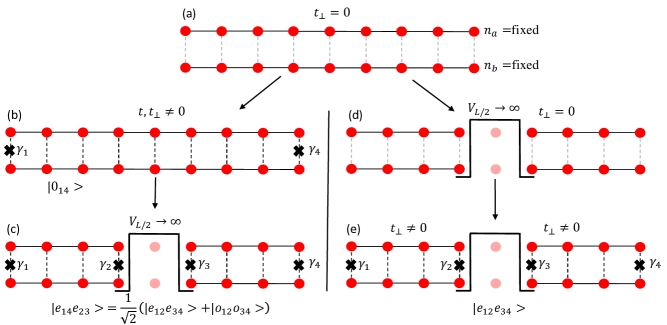
Figure 3: Implementation of a fusion-testing protocol analogous to Ref. [Aasen et al., 2016] in a cold atom setting with particle number conservation. (a) Two disconnected chains with $t_{\perp}=0$ and a fixed number of particles in each chain $n_{a},n_{b}$. (b) By turning on the inter-chain coupling $t_{\perp}$ the system is driven to the doubly degenerate state with well defined parity state of Majorana operators $i\gamma_{1}\gamma_{4}=+1$ dented $|e_{14}\rangle$. (c) A strong potential barrier is created in the center. The resulting central region has a trivial gap, similar to the regions at $x<0$ and $x>L$. Thus an additional degeneracy emerges described by two additional Majorana operators $\gamma_{2},\gamma_{3}$ which have been created from the vacuum in an even parity state $|e_{23}\rangle$. As described in Eq. (17) this is a maximally entangled state in terms of the parity of the left and right sides. (d,e) To test that parity fluctuations in each subregion are intrinsic to the system, we can prepare a system described by the same four Majorana operators but with a well defined parity in each half, by first breaking the decoupled chains into two separate segments each (d), and then turning on the inter-chain coupling $t_{\perp}$ (e).

V Conclusions

In this work we described a closed, particle-conserving setup in a cold atom system endowed with both a synthetic dimension and a synthetic gauge field with the goal of realizing close analogues of Majorana zero modes. In contrast to other approaches relying on the superconducting proximity effect, the two-particle hopping process, which is responsible for the topological superconducting phase, is generated in our setup from the single particle hopping in the presence of small attractive interaction. We emphasize, that our model builds upon an experimentally tested implementation of quantum Hall edge states in the cold atom setting.

The synthetic dimension approach has a number of advantages. Local particle-particle interactions in real space become non-local in the synthetic dimension. This is the key feature which effectively turns a small local attractive interaction into an attractive interaction between “distant” edge states in a synthetic quantum Hall ribbon, thus resulting in the formation of analogues of Majorana zero modes. The wavefunction of these modes, while local in the real space, remains non-local in the synthetic dimension. The prerequisite non-local interactions can not be induced in a conventional condensed matter setup.

The fact that Majorana operators are non-local in the synthetic dimension allows us to manipulate the associated degeneracy by adding a synthetic flux $\Phi_{x}$. This in turn can provide us with a useful knob for combining “topological” and “non-topological” qubit operations. An even more intriguing possibility is to utilize a similar setup for producing and manipulating fractionalized zero modes Clarke et al. (2013); Lindner et al. (2012); Cheng (2012); Alicea and Fendley (2016), a topic that we intend to cover elsewhere.

VI Acknowledgments

The authors would like to thank Hans Peter Büchler, Sebastian Diehl, Yuval Gefen, Leonardo Mazza, and Christophe Mora for useful discussion. This project was supported in part by the ISF Grant No. 1243/13 and by the BSF Grant No. 2016255; KS was supported in part by the NSF DMR-1411359 grant.

Appendix A Matrix elements of $\mathcal{H}_{\perp}$

Our goal is to compute matrix elements of $\mathcal{H}_{\perp}(x)$ in the ground state manifold. To set up the notation, we write the mode expansion (in this appendix we set $\theta=\sqrt{K_{-}}\theta_{-}$, $\varphi=\varphi_{-}/\sqrt{K_{-}}$, $v_{-}=v$)

$$\varphi(t,x)=\varphi_{0}+\sum_{k\neq 0}\frac{1}{\sqrt{4\pi|n|}}\left(\beta_{n}e^{ik_{n}x-iv|k_{n}|t}+h.c.\right),$$ (18)

where $k_{n}=\frac{2\pi n}{L}$ and $[\beta_{n},\beta_{n^{\prime}}]=\delta_{n,n^{\prime}}$. The free Hamiltonian is $H_{0}=\frac{v}{2}\int_{0}^{L}dx[(\partial_{x}\varphi)^{2}+\Pi^{2}]$ with the conjugate field $\Pi(t,x)=\frac{1}{v}\partial_{t}\varphi(t,x)$ satisfying $[\varphi(t,x),\Pi(t,y)]=i\delta(x-y)$. We define also $\Pi(t,x)=-\partial_{x}\theta(x)$. One can check that these canonical commutation relations are recovered using the mode expansion and that the Hamiltonian becomes $H_{0}=\frac{2\pi v}{L}\sum_{n=1}^{\infty}n[\beta_{n}^{\dagger}\beta_{n}+\beta_{-n}^{\dagger}\beta_{-n}]$.

We consider the interface $x=0$ between the region where $\theta$ is pinned $\theta(x)=\sqrt{\pi/2}~{}n_{\theta}$ for $x>0$, and $\varphi$ is pinned to $\varphi(x)=\sqrt{2\pi}n_{\varphi}^{L}$ for $x<0$. The latter is accounted for by the boundary condition $\varphi(x=0,t)=\sqrt{2\pi}n_{\varphi}^{L}$. Using the mode expansion, this boundary condition implies $\beta_{n}+\beta_{-n}=0$, hence

$$\varphi(t,x) = \sqrt{2\pi}n_{\varphi}^{L}+i\sum_{k\neq 0}\frac{1}{\sqrt{\pi n}}\sin(k_{n}x)\left(\beta_{n}-\beta_{n}^{\dagger}\right),$$

$$\theta(t,x) = \sum_{k\neq 0}\frac{1}{\sqrt{\pi n}}\cos(k_{n}x)\left(\beta_{n}+\beta_{n}^{\dagger}\right).$$ (19)

Ignoring tunneling between minima $\theta(x)=\sqrt{\pi/2}~{}n_{\theta}$ of the cosine potential in the region $x>0$, we replace the latter by a mass term $g(\theta-\sqrt{\pi/2}~{}n_{\theta})^{2}$ (where $g\rightarrow\tilde{g}=g/K_{-}$). This gives a finite average value $\langle\theta(x)\rangle=\sqrt{\pi/2}~{}n_{\theta}$. To account for fluctuations around this value, we rewrite the Hamiltonian using the mode expansion:

$$H_{n_{\theta}}=\sum_{n=1}^{\infty}[A_{n}(\beta^{\dagger}_{n}\beta_{n}+\beta_{n}\beta_{n}^{\dagger})+B_{n}(\beta_{n}^{2}+(\beta_{n}^{\dagger})^{2})],$$ (20)

where $A_{n}=vk_{n}+B_{n}$, $B_{n}=g/k_{n}$. After a Bogoliubov transformation one obtains $H=\sum_{n}E_{n}b_{n}^{\dagger}b_{n}$ where $\beta_{n}=f_{n}b_{n}+g_{n}b_{n}^{\dagger}$, $f_{n}=\sqrt{\frac{1}{2}\left(\frac{A_{n}}{E_{n}}+1\right)}$, $g_{n}=-\sqrt{\frac{1}{2}\left(\frac{A_{n}}{E_{n}}-1\right)}$, ${E_{n}^{2}=A_{n}^{2}-B_{n}^{2}}$. The Hamiltonian $H_{n_{\theta}}$ describes excitations above the $|n_{\theta}\rangle$ ground state.

Having argued that $\mathcal{H}_{\perp}$ is diagonal in this basis, we will evaluate

$$\langle n_{\theta}|\mathcal{H}_{\perp}(x)|n_{\theta}\rangle=t_{\perp}e^{i\Phi_{x}/2}\langle n_{\theta}|R^{\dagger}_{a}R_{b}|n_{\theta}\rangle\\ +t_{\perp}e^{-i\Phi_{x}/2}\langle n_{\theta}|L^{\dagger}_{a}L_{b}|n_{\theta}+c.c.\rangle$$ (21)

This requires calculating quantities such as

$$\langle n_{\theta}|R^{\dagger}_{a}R_{b}|n_{\theta}\rangle=\frac{1}{\pi a_{0}}\langle n_{\theta}|e^{-i\sqrt{\frac{2\pi}{K_{-}}}(\theta(x)+K_{-}\varphi(x))}|n_{\theta}\rangle.$$

Introducing a shorthand notation $\langle...\rangle\equiv\langle n_{\theta}|...|n_{\theta}\rangle$ and using $\langle e^{A}\rangle=e^{\langle A\rangle}e^{\frac{1}{2}\langle(A-\langle A\rangle)^{2}\rangle}$, we have

$$\langle e^{i\sqrt{\frac{2\pi}{K_{-}}}(\theta+K_{-}\varphi)}\rangle=e^{i\pi n_{\theta}}e^{-\pi/K_{-}(\langle(K_{-}\varphi+\theta)^{2}\rangle-(\langle K_{-}\varphi+\theta\rangle)^{2}}.$$ (22)

Computing the fluctuations using Eq. (A) we obtain

$$\langle e^{i\sqrt{\frac{2\pi}{K_{-}}}(\theta(x)+K_{-}\varphi(x))}\rangle=e^{i\pi n_{\theta}}e^{-\pi{\text{var}}(\theta_{-}(x))-\pi{\text{var}}(\varphi_{-}(x))},$$ (23)

and

$${\text{var}}(\theta(x))=\sum_{n=1}^{\infty}\frac{\cos^{2}(k_{n}x)}{\pi n}\frac{vk_{n}}{\sqrt{(vk_{n})^{2}+2gv}},$$

$${\text{var}}(\varphi(x))=\sum_{n=1}^{\infty}\frac{\sin^{2}(k_{n}x)}{\pi n}\frac{vk_{n}+\frac{2g}{k_{n}}}{\sqrt{(vk_{n})^{2}+2gv}}.$$ (24)

One can see a length scale $\xi=\sqrt{\frac{vK_{-}}{2g}}$. Evaluating these sums for $\xi\ll x\ll L$ gives

$${\text{var}}(\theta_{-}(x)) \sim \frac{1}{2\pi K_{-}}{\text{log}}(\xi/a_{0}),$$

$${\text{var}}(\varphi_{-}(x)) \sim \frac{K_{-}}{2\pi}{\text{log}}(\xi/a_{0})+\frac{1}{2}\frac{xK_{-}}{\xi}.$$ (25)

One can see then that

$$\langle n_{\theta}|R^{\dagger}_{a}R_{b}|n_{\theta}\rangle=\langle n_{\theta}|L^{\dagger}_{a}L_{b}|n_{\theta}\rangle\\ =\frac{e^{i\pi n_{\theta}}e^{-\pi xK_{-}/(2\xi)}a_{0}^{1/2K_{-}+K_{-}/2-1}}{\pi\xi^{1/2K_{-}+K_{-}/2}}$$ (26)

The result of the calculation is then

$$\langle n_{\theta}|\mathcal{H}_{\perp}(x)|n_{\theta}\rangle\\ =\frac{2t_{\perp}e^{i\pi n_{\theta}}e^{-\pi xK_{-}/(2\xi)}a_{0}^{1/2K_{-}+K_{-}/2-1}\cos(\Phi_{x}/2)}{\pi\xi^{1/2K_{-}+K_{-}/2}}.$$ (27)

Integrating over $x$ one obtains

$$\langle n_{\theta}|H_{\perp}|n_{\theta}\rangle\\ =\frac{4t_{\perp}}{\pi^{2}K_{-}}\cos(\Phi_{x}/2)e^{i\pi n_{\theta}}\left(\frac{a_{0}}{\xi}\right)^{1/2K_{-}+K_{-}/2-1}.$$ (28)

Appendix B Fusion protocol within an exactly solvable particle-number conserving model

In order to better understand the physics of the fusion process in our model, we turn to an exactly-solvable toy model Iemini et al. (2015), which is particle-number conserving as well. We begin by reviewing the construction of the model Iemini et al. (2015), and then we describe the fusion process.

The well known Kitaev model Kitaev (2001) is a non particle-number conserving model whose Hamiltonian is

$$H_{K}=\sum\limits_{j}\left(-Ja_{j}^{\dagger}a_{j+1}-\Delta a_{j}a_{j+1}+h.c.-\mu(n_{j}-\frac{1}{2})\right).$$ (29)

It is exactly solvable and at the “sweet spot” in the parameter space where $\mu=0$, and $\Delta=J>0$ (we set $\Delta=J=1$), it is diagonalized as $H_{K}=\sum_{j}\ell^{\dagger}_{j}\ell_{j}$, where $\ell_{j}=C^{\dagger}_{j}+A_{j}$, $C^{\dagger}_{j}=a^{\dagger}_{j}+a^{\dagger}_{j+1}$, and $A_{j}=a_{j}-a_{j+1}$. In order to construct a number conserving model out of the Kitaev model, we recall that in BCS theory we begin with a number-conserving, quartic Hamiltonian, and then by employing a mean field description, we turn into a quadratic Hamiltonian and lose number conservation. Analogously, one can write the quartic Hamiltonian $H_{a}=\sum\limits_{j}L^{\dagger}_{j}L_{j}$, where $L_{j}=C^{\dagger}_{j}A_{j}$. It is immediate to see that this model is number conserving. Also the ground state of the Kitaev model satisfying $\ell_{j}|\text{GS}_{K}\rangle=0$, is the ground state of this model as well since $L_{j}|\text{GS}_{K}\rangle=C_{j}^{\dagger}A_{j}|\text{GS}_{K}\rangle=C_{j}^{\dagger}C_{j}^{\dagger}|\text{GS}_{K}\rangle=0$. In fact, one can project from the model states with well defined number of particles, each of which is a ground state of $H_{a}$.

The next step is to create an interacting two-chain version of this model. Denoting the chains by an extra subscript $a,b$, we do this by adding an interaction term - $L_{I,j}=C^{\dagger}_{a,j}A_{b,j}+C^{\dagger}_{b,j}A_{a,j}$. This interaction term is selected since it annihilates the Kitaev ground state as well, while conserving the total particle number.

We can use this model to better understand the fusion process in our setup. The fusion/splitting processes can be modeled by making coupling constants for the central links $(\alpha=a,b)$ as well as central plaquette $(\alpha=I)$ time dependent:

$$\hat{H}=\sum\limits_{\alpha=a,b,I}\sum\limits_{j\neq\ell/2}^{\ell-1}\hat{L}^{\dagger}_{\alpha,j}\hat{L}_{\alpha,j}+g(t)\sum\limits_{\alpha=a,b,I}\hat{L}^{\dagger}_{\alpha,\ell/2}\hat{L}_{\alpha,\ell/2},$$ (30)

where $a,b$ label different chains and $\ell$ is the chain lenth (assumed to be even). Initially $g(0)=1$, corresponding to a uniform system, and eventually $g(t\to\infty)=0$, corresponding to two decoupled halves. It is important to notice that each single term in this Hamiltonian annihilates the ground state. Hence, if we begin in a ground state, the time dependent Schrödinger equation trivially guarantees that we remain in the same ground state. Therefore for this specific model we need not assume anything about the functional form of the time dependence $g(t)$.

The ground states of this Hamiltonian at $g=1$ are characterized by the total number of particles $N$, and by the parity of the two chains, being both even or both odd for an even number of particles, or one even and one odd if $N$ is odd. They are given by

$$\begin{gathered}|\psi_{\ell}(N)\rangle_{ee}=\mathcal{N}^{-1/2}_{ee,\ell,N}\sum\limits_{n=0}^{N/2}\sum\limits_{\begin{subarray}{c}\{\vec{j}_{2n}\}\\ \{\vec{q}_{N-2n}\}\end{subarray}}|\vec{j}_{2n}\rangle\otimes|\vec{q}_{N-2n}\rangle,\\ |\psi_{\ell}(N)\rangle_{oo}=\mathcal{N}^{-1/2}_{oo,\ell,N}\sum\limits_{n=0}^{N/2-1}\sum\limits_{\begin{subarray}{c}\{\vec{j}_{2n+1}\}\\ \{\vec{q}_{N-2n-1}\}\end{subarray}}|\vec{j}_{2n+1}\rangle\otimes|\vec{q}_{N-2n-1}\rangle.\end{gathered}$$ (31)

where $\vec{j}_{m},\vec{q}_{m}$ are m-sized vectors denoting the ordered locations of particles on the $a$ and $b$ chains respectively, and the sum is over all possible configurations,

$$\mathcal{N}_{ee,\ell,N} = \sum_{n=0}^{N/2}\binom{\ell}{2n}\binom{\ell}{N-2n},~{}~{}(N~{}{\rm{even}})$$

$$\mathcal{N}_{oo,\ell,N} = \sum_{n=0}^{N/2-1}\binom{\ell}{2n+1}\binom{\ell}{N-2n-1}.$$ (32)

Similarly for $N$ odd the number of configurations with well defined parities in each chain is

$$\mathcal{N}_{eo,\ell,N}=\mathcal{N}_{oe,\ell,N}=\sum_{n=0}^{(N-1)/2}\binom{\ell}{2n}\binom{\ell}{N-2n}.~{}~{}(N~{}{\rm{odd}})$$

In the end of the fusion process $g=0$ and the system separates into two halves. Since the wave function in this model does not change at all, in order to describe the final state we simply perform a left-right decomposition of the ground state wave function. We assume that the total number of particles $N$ as well as well as the number of particles in each individual chain is even. Since the system remains in the zero-energy ground state of the decoupled left-right Hamiltonians, it is guaranteed that we can use the same ground states Eq. (31) of the two half-systems $\ell\to\ell/2$. We find that the decomposition is given by

$$|\psi_{\ell}(N)\rangle_{ee}=\sum\limits_{\mu=e,o}\sum\limits_{\begin{subarray}{c}N_{L}=0\end{subarray}}^{N}A_{N_{L},\mu\mu^{\prime}}|\psi^{L}_{\ell/2}(N_{L})\rangle_{\mu\mu^{\prime}}\\ \otimes|\psi^{R}_{\ell/2}(N-N_{L})\rangle_{\mu\mu^{\prime}},$$ (33)

Here $N_{L}$ is the charge of the left part of the system. Writing

$$N=n_{a}+n_{b},~{}N_{L}=n_{a}^{L}+n_{b}^{L},~{}~{}~{}N-N_{L}=n_{a}^{R}+n_{b}^{R},$$ (34)

since we assumed $n_{a}$ and $n_{b}$ are even, the parity of $n_{a}^{L}$ equals that of $n_{a}^{R}$ and is denoted $\mu$; then the equal parities of $n_{b}^{L}$ and $n_{b}^{R}$ which are denoted $\mu^{\prime}$ equal

$$\mu^{\prime}=\mu({\rm{for}}~{}N_{L}~{}{\rm{even}}),~{}~{}~{}\mu^{\prime}=\bar{\mu}~{}{\rm{for}}~{}N_{L}~{}{\rm{odd}},$$ (35)

with $\bar{o}=e$ and $\bar{e}=o$. The coefficients are given by $A_{N_{L},\mu\mu^{\prime}}=\sqrt{\frac{\mathcal{N}_{\mu\mu^{\prime},\ell/2,N_{L}}\mathcal{N}_{\mu\mu^{\prime},\ell/2,N-N_{L}}}{\mathcal{N}_{ee,\ell,N}}}$. In fact the dependence of these coefficients on $\mu,\mu^{\prime}$ becomes exponentially small with increasing system size. Ignoring these exponentially small effects we have $A_{N_{L},\mu\mu^{\prime}}=A_{N_{L}}$ and can therefore write

$$|\psi_{\ell}(N)\rangle_{ee}\\ =\sum\limits_{\begin{subarray}{c}N_{L}=\text{even}\end{subarray}}A_{N_{L}}\left[|\psi^{L}_{\ell/2}(N_{L})\rangle_{ee}\otimes|\psi^{R}_{\ell/2}(N-N_{L})\rangle_{ee}\right.\\ +\left.|\psi^{L}_{\ell/2}(N_{L})\rangle_{oo}\otimes|\psi^{R}_{\ell/2}(N-N_{L})\rangle_{oo}\right]\\ +\sum\limits_{\begin{subarray}{c}N_{L}=\text{odd}\end{subarray}}A_{N_{L}}\left[|\psi^{L}_{\ell/2}(N_{L})\rangle_{eo}\otimes|\psi^{R}_{\ell/2}(N-N_{L})\rangle_{eo}\right.\\ +\left.|\psi^{L}_{\ell/2}(N_{L})\rangle_{oe}\otimes|\psi^{R}_{\ell/2}(N-N_{L})\rangle_{oe}\right]$$ (36)

We can now explicitly see that for each particle number $N_{L}$ in the left segment, the parity of each individual chain is not well defined and is in fact entangled between the left and right sides in accordance to the fusion rules for Majorana zero modes $\gamma_{3},\gamma_{4}$.

However one should note a peculiarity of this model. In this equation all charge states are equally likely. The degeneracy of the system is extensive as all these states differing by $N_{L}$ are degenerate, in addition to the degeneracy associated with the parity of each chain in each side, attributed to Majorana operators. In any generic system like the one considered in the main text, these states differing by $N_{L}$ are non-degenerate and actually have an energy difference which scales with the system size as power law. This can be understood using bosonization. While the odd sector is gapped everywhere, either by pair tunneling in the superconductor regions or by the mass term in the trivial regions, the even sector, i.e. the charge sector, is only gapped in the trivial regions. The superconductor regions act as Luttinger liquids for the charge sector. Hence they provide a finite stiffness, which favors a state with a fixed charge.

References

- Nayak et al. (2008) C. Nayak, S. H. Simon, A. Stern, M. Freedman, and S. Das Sarma, Rev. Mod. Phys. 80, 1083 (2008), arXiv:0707.1889 .
- Alicea (2012) J. Alicea, Rep. Prog. Phys. 75, 076501 (2012), arXiv:1202.1293 .
- Beenakker (2013) C. W. J. Beenakker, Annu. Rev. Condens. Matter Phys. 4, 113 (2013), arXiv:1112.1950 .
- Goldman et al. (2016) N. Goldman, J. C. Budich, and P. Zoller, Nat. Phys. 12, 639 (2016), arXiv:1607.03902 .
- Celi et al. (2014) A. Celi, P. Massignan, J. Ruseckas, N. Goldman, I. B. Spielman, G. Juzeliūnas, and M. Lewenstein, Phys. Rev. Lett. 112, 043001 (2014), arXiv:1307.8349 .
- Mancini et al. (2015) M. Mancini, G. Pagano, G. Cappellini, L. Livi, M. Rider, J. Catani, C. Sias, P. Zoller, M. Inguscio, M. Dalmonte, and L. Fallani, Science 349, 1510 (2015), arXiv:1502.02495 .
- Stuhl et al. (2015) B. K. Stuhl, H.-I. Lu, L. M. Aycock, D. Genkina, and I. B. Spielman, Science 349, 1514 (2015), arXiv:1502.02496 .
- Price et al. (2015) H. M. Price, O. Zilberberg, T. Ozawa, I. Carusotto, and N. Goldman, Phys. Rev. Lett. 115, 195303 (2015), arXiv:1505.04387 .
- Barbarino et al. (2015) S. Barbarino, L. Taddia, D. Rossini, L. Mazza, and R. Fazio, Nat. Commun. 6, 8134 (2015), arXiv:1504.00164 .
- Zeng et al. (2015) T.-S. Zeng, C. Wang, and H. Zhai, Phys. Rev. Lett. 115, 095302 (2015), arXiv:1504.02263 .
- Taddia et al. (2017) L. Taddia, E. Cornfeld, D. Rossini, L. Mazza, E. Sela, and R. Fazio, Phys. Rev. Lett. 118, 230402 (2017), arXiv:1607.07842 .
- Petrescu and Le Hur (2015) A. Petrescu and K. Le Hur, Phys. Rev. B 91, 054520 (2015), arXiv:1410.6105 .
- Cornfeld and Sela (2015) E. Cornfeld and E. Sela, Phys. Rev. B 92, 115446 (2015), arXiv:1506.08461 .
- Calvanese Strinati et al. (2017) M. Calvanese Strinati, E. Cornfeld, D. Rossini, S. Barbarino, M. Dalmonte, R. Fazio, E. Sela, and L. Mazza, Phys. Rev. X 7, 021033 (2017), arXiv:1612.06682 .
- Petrescu et al. (2017) A. Petrescu, M. Piraud, G. Roux, I. P. McCulloch, and K. Le Hur, Phys. Rev. B 96, 014524 (2017), arXiv:1612.05134 .
- Fu and Kane (2008) L. Fu and C. L. Kane, Phys. Rev. Lett. 100, 096407 (2008), arXiv:0707.1692 .
- Lutchyn et al. (2010) R. M. Lutchyn, J. D. Sau, and S. Das Sarma, Phys. Rev. Lett. 105, 077001 (2010), arXiv:1002.4033 .
- Oreg et al. (2010) Y. Oreg, G. Refael, and F. von Oppen, Phys. Rev. Lett. 105, 177002 (2010), arXiv:1003.1145 .
- Clarke et al. (2013) D. J. Clarke, J. Alicea, and K. Shtengel, Nat. Commun. 4, 1348 (2013), arXiv:1204.5479 .
- Lindner et al. (2012) N. H. Lindner, E. Berg, G. Refael, and A. Stern, Phys. Rev. X 2, 041002 (2012), arXiv:1204.5733 .
- Cheng (2012) M. Cheng, Phys. Rev. B 86, 195126 (2012), arXiv:1204.6084 .
- Alicea and Fendley (2016) J. Alicea and P. Fendley, Annu. Rev. Condens. Matter Phys. 7, 119 (2016), arXiv:1504.02476 .
- Cheng and Tu (2011) M. Cheng and H.-H. Tu, Phys. Rev. B 84, 094503 (2011).
- Sau et al. (2011) J. D. Sau, B. I. Halperin, K. Flensberg, and S. Das Sarma, Phys. Rev. B 84, 144509 (2011), arXiv:1106.4014 .
- Kraus et al. (2013) C. V. Kraus, M. Dalmonte, M. A. Baranov, A. M. Läuchli, and P. Zoller, Phys. Rev. Lett. 111, 173004 (2013), arXiv:1302.0701 .
- Ruhman et al. (2015) J. Ruhman, E. Berg, and E. Altman, Phys. Rev. Lett. 114, 100401 (2015), arXiv:1412.3444 .
- Iemini et al. (2015) F. Iemini, L. Mazza, D. Rossini, R. Fazio, and S. Diehl, Phys. Rev. Lett. 115, 1 (2015), arXiv:1504.04230 .
- Mazza et al. (2015) L. Mazza, M. Aidelsburger, H.-H. Tu, N. Goldman, and M. Burrello, New J. Phys. 17, 105001 (2015), arXiv:1506.08057 .
- Chen et al. (2017) C. Chen, W. Yan, C. Ting, Y. Chen, and F. Burnell, arXiv:1701.01794 (2017).
- Guther et al. (2017) K. Guther, N. Lang, and H. P. Büchler, Phys. Rev. B 96, 121109 (2017), arXiv:1705.01786 .
- Yan et al. (2015) Z. Yan, S. Wan, and Z. Wang, Sci. Rep. 5, 15927 (2015), arXiv:1504.03223 .
- Kitaev (2001) A. Y. Kitaev, Phys.-Usp. 44, 131 (2001), arXiv:cond-mat/0010440 .
- Klinovaja and Loss (2013) J. Klinovaja and D. Loss, Phys. Rev. Lett. 110, 126402 (2013).
- Su et al. (1980) W. P. Su, J. R. Schrieffer, and A. J. Heeger, Phys. Rev. B 22, 2099 (1980).
- Kane et al. (2002) C. L. Kane, R. Mukhopadhyay, and T. C. Lubensky, Phys. Rev. Lett. 88, 036401 (2002), cond-mat/0108445 .
- Keselman and Berg (2015) A. Keselman and E. Berg, Phys. Rev. B 91, 235309 (2015), arXiv:1502.02037 .
- Note (1) For finite density mismatch the integer-valued operators are defined in the same way in terms of rather than .
- Haim et al. (2016) A. Haim, K. Wölms, E. Berg, Y. Oreg, and K. Flensberg, Phys. Rev. B 94, 115124 (2016), arXiv:1605.09385 .
- Atala et al. (2014) M. Atala, M. Aidelsburger, M. Lohse, J. T. Barreiro, B. Paredes, and I. Bloch, Nat. Phys. 10, 588 (2014), arXiv:1402.0819 .
- Aasen et al. (2016) D. Aasen, M. Hell, R. V. Mishmash, A. Higginbotham, J. Danon, M. Leijnse, T. S. Jespersen, J. A. Folk, C. M. Marcus, K. Flensberg, and J. Alicea, Phys. Rev. X 6, 031016 (2016), arXiv:1511.05153 .
- Kraus et al. (2012) C. V. Kraus, S. Diehl, P. Zoller, and M. A. Baranov, New J. Phys. 14, 113036 (2012), arXiv:1201.3253 .