Probing SUSY effects in ${K_{S}^{0}\rightarrow\mu^{+}\mu^{-}}$

Abstract

We explore supersymmetric contributions to the decay $K_{S}^{0}\rightarrow\mu^{+}\mu^{-}$, in light of current experimental data. The Standard Model (SM) predicts $\mathcal{B}(K_{S}^{0}\rightarrow\mu^{+}\mu^{-})\approx 5\times 10^{-12}$. We find that contributions arising from flavour violating Higgs penguins can enhance the branching fraction up to $\approx 35\times 10^{-12}$ within different scenarios of the Minimal Supersymmetric Standard Model (MSSM), as well as suppress it down to $\approx 0.78\times 10^{-12}$. Regions with fine-tuned parameters can bring the branching fraction up to the current experimental upper bound, $8\times 10^{-10}$. The mass degeneracy of the heavy Higgs bosons in MSSM induces correlations between $\mathcal{B}(K_{S}^{0}\rightarrow\mu^{+}\mu^{-})$ and $\mathcal{B}(K_{L}^{0}\rightarrow\mu^{+}\mu^{-})$. Predictions for the $CP$ asymmetry in $K^{0}\rightarrow\mu^{+}\mu^{-}$ decays in the context of MSSM are also given, and can be up to eight times bigger than in the SM.

1 Introduction

Leptonic decays of pseudoscalar mesons with down-type quarks are known to be very sensitive to the Higgs sector of the Minimal Supersymmetric Standard Model (MSSM), due to, among others, enhancement factors proportional to $\left(\tan^{6}\beta/M_{A}^{4}\right)$. This factor comes from the so-called non-holomorphic Yukawa terms at large $\tan\beta$ Hamzaoui:1998nu ; Babu:1999hn ; Chankowski:2000ng ; Bobeth:2001sq ; Isidori:2001fv ; Isidori:2002qe , which are triggered by the supersymmetric (SUSY) $\mu$ term, and hence the non-SUSY two-Higgs-doublet model cannot produce this enhancement Isidori:2001fv . The best known example is $B_{s}^{0}\rightarrow\mu^{+}\mu^{-}$ Hamzaoui:1998nu ; Babu:1999hn ; Chankowski:2000ng ; Bobeth:2001sq ; Isidori:2001fv ; Isidori:2002qe ; Choudhury:1998ze ; Huang:2000sm ; Xiong:2001up ; Dedes:2001fv ; Bobeth:2002ch ; Baek:2002rt ; Dedes:2002zx ; Mizukoshi:2002gs ; Baek:2002wm . If Minimal Flavour Violation (MFV) is imposed, then $B_{s}^{0}\rightarrow\mu^{+}\mu^{-}$ is the dominant constraint in $P\rightarrow\mu^{+}\mu^{-}$ decays. This is due to the stronger Yukawa coupling of the $b$–quark compared to the $s$–quark, and to the better experimental precision in $B_{s}^{0}\rightarrow\mu^{+}\mu^{-}$ compared to $B_{d}^{0}\rightarrow\mu^{+}\mu^{-}$. However, in the presence of new sources of flavour violation, the sensitivity of each mode depends on the flavour and $CP$ structures of the corresponding terms. Hence, a priori, $B_{s}^{0}\rightarrow\mu^{+}\mu^{-}$, $B_{d}^{0}\rightarrow\mu^{+}\mu^{-}$, $K_{S}^{0}\rightarrow\mu^{+}\mu^{-}$, and $K_{L}^{0}\rightarrow\mu^{+}\mu^{-}$ are all separate constraints that carry complementary information in the general MSSM. The observables related to these decay modes are typically branching fractions and $CP$ asymmetries. Even though the muon polarization could carry interesting information, it cannot be observed by current experiments.

In this paper, we focus on the MSSM effects in the $K_{S}^{0}\rightarrow\mu^{+}\mu^{-}$ decay. The Standard Model (SM) expectation is $(5.18\pm 1.50_{\textrm{LD}}\pm 0.02_{\textrm{SD}})\times 10^{-12}$ Ecker:1991ru ; Isidori:2003ts ; DAmbrosio:2017klp , where the first uncertainty comes from the long-distance (LD) contribution and the second one comes from the short-distance (SD) contribution. On the other hand, the current experimental upper bound is $8\times 10^{-10}$ at $90\%$ C.L., using $3$ fb^-1 of LHCb data LHCb:KsMuMu . The LHCb upgrade could reach sensitivities at the level of about $1\times 10^{-11}$ or even below, approaching the SM prediction DMS_FPCP .

We predict the branching ratio $\mathcal{B}(K_{S}^{0}\rightarrow\mu^{+}\mu^{-})$ under consideration of MSSM contributions and taking into account the relevant experimental constraints on the branching fractions $\mathcal{B}(K_{L}^{0}\rightarrow\mu^{+}\mu^{-})$, $\mathcal{B}(B^{+}\rightarrow\tau^{+}\nu_{\tau})$ and $\mathcal{B}(K^{+}\rightarrow\mu^{+}\nu_{\mu})$, the $CP$ violation parameters $\varepsilon^{\prime}_{K}/\varepsilon_{K}$ and $\varepsilon_{K}$, the $K^{0}_{L}$–$K^{0}_{S}$ mass difference, $\Delta M_{K}\equiv M_{K^{0}_{L}}-M_{K^{0}_{S}}>0$, and the Wilson coefficient $C_{7}$ from $b\rightarrow s\gamma$. We use the Mass Insertion Approximation (MIA) MassInsertion , treating the mass insertion terms as phenomenological parameters at the SUSY scale. The details of the formalism are given in section 2. The subsets of the MSSM parameter space are studied in scans performed on Graphics Processing Units (GPU), as detailed in section 3. The results are shown in section 4 and conclusions are drawn in section 5.

2 Formalism

2.1 Definitions

In this paper, we follow the notations of refs. Altmannshofer:2009ne ; Rosiek:1995kg . We denote the right-handed down and up squarks as $D$ and $U$. On the other hand, the two left-handed squarks have the same mass because of the $\textrm{SU}(2)_{L}$ doublet, and they are denoted as $Q$. The average of the $Q$, $D$, and $U$-squark masses squared are denoted by $\tilde{m}^{2}_{Q}$, $\tilde{m}^{2}_{d}$, $\tilde{m}^{2}_{u}$, respectively.

The mass insertions (hereafter MIs) are defined as:

$$\left(\delta_{d}^{LL}\right)_{ij} =\frac{\left[\left(\mathcal{M}_{D}^{2}\right)_{LL}\right]_{ij}}{\tilde{m}_{Q}^{2}}=\frac{(m^{2}_{Q})_{ji}}{\tilde{m}_{Q}^{2}},$$ (2.1)

$$\left(\delta_{u}^{LL}\right)_{ij} =\frac{\left[\left(\mathcal{M}_{U}^{2}\right)_{LL}\right]_{ij}}{\tilde{m}_{Q}^{2}}=\frac{(Vm^{2}_{Q}V^{{\dagger}})_{ji}}{\tilde{m}_{Q}^{2}},$$ (2.2)

$$\left(\delta_{d}^{RR}\right)_{ij} =\frac{\left[\left(\mathcal{M}_{D}^{2}\right)_{RR}\right]_{ij}}{\tilde{m}_{d}^{2}}=\frac{(m^{2}_{D})_{ij}}{\tilde{m}_{d}^{2}},$$ (2.3)

where $V$ is the Cabibbo–Kobayashi–Maskawa (CKM) matrix and $\mathcal{M}^{2}_{D,U}$ are the $6\times 6$ squark mass matrices. Note that the indices $ij$ are inverted for $LL$. Comparison with the SUSY Les Houches Accord 2 convention Allanach:2008qq is given in the appendix of ref. Altmannshofer:2009ne .

The running coupling constants $\alpha_{1}$, $\alpha_{2}$, and $\alpha_{3}$ are defined as

$$\alpha_{1} =\frac{g_{1}^{2}}{4\pi}=\frac{5}{3}\frac{g^{\prime 2}}{4\pi},$$ (2.4)

$$\alpha_{2} =\frac{g_{2}^{2}}{4\pi}=\frac{g^{2}}{4\pi},$$ (2.5)

$$\alpha_{3} =\frac{g_{3}^{2}}{4\pi}=\frac{g_{s}^{2}}{4\pi},$$ (2.6)

where $g^{\prime}$, $g$, and $g_{s}$ are the $\textrm{U}(1)_{Y}$, $\textrm{SU}(2)_{L}$, and $\textrm{SU}(3)_{C}$ group coupling constants, respectively. In the following, these couplings are evaluated at the $\mu^{\textrm{SUSY}}$ scale, where we define $\mu^{\textrm{SUSY}}=\sqrt{\tilde{m}_{Q}M_{3}}$.

2.2 Observables

As will be shown in the next subsections, the main MSSM contribution to $\mathcal{B}(K_{S}^{0}\rightarrow\mu^{+}\mu^{-})$ is proportional to $\left[\left(\delta_{d}^{LL(RR)}\right)_{12}\mu\tan^{3}\beta M_{3}/M_{A}^{2}\right]^{2}$. In order to constrain those parameters, the following observables are calculated in addition to $\mathcal{B}(K_{S}^{0}\rightarrow\mu^{+}\mu^{-})$:

• Observables sensitive, among others, to the off-diagonal mass insertion terms $\left(\delta_{d}^{LL(RR)}\right)_{12}$:
  $\mathcal{B}(K_{L}^{0}\rightarrow\mu^{+}\mu^{-})$ , $\varepsilon^{\prime}_{K}/\varepsilon_{K}$, $\varepsilon_{K}$, and $\Delta M_{K}$.

• Observables sensitive to $\tan\beta$ and the heavy Higgs mass: $\mathcal{B}(B^{+}\rightarrow\tau^{+}\nu_{\tau})$, $\mathcal{B}(K^{+}\rightarrow\mu^{+}\nu_{\mu})$, $\Delta C_{7}$.

The definitions of $\mathcal{B}(B^{+}\rightarrow\tau^{+}\nu_{\tau})$, $\mathcal{B}(K^{+}\rightarrow\mu^{+}\nu_{\mu})$, and $C_{7}$ are given in ref. Altmannshofer:2009ne and the remaining observables are defined in the following subsections. The CKM matrix is fitted excluding measurements with potential sensitivity to MSSM contributions.

The constraints we impose on physics observables sensitive to the MSSM same parameters as $\mathcal{B}(K_{S}^{0}\rightarrow\mu^{+}\mu^{-})$ are listed in table 1, where the EXP/SM represents the measured value over the SM prediction with their uncertainties. Due to the poor theoretical knowledge of $\Delta M_{K}$, we assign a $100\%$ theoretical uncertainty; thus, the constraint imposed on this observable penalizes only $\mathcal{O}$(1) effects. It is not counted as a degree of freedom in the $\chi^{2}$ tests, so that the $\Delta M_{K}$ constraint can only make the bounds tighter, but never looser. Remaining constraints can in principle be satisfied by adjusting the other parameters of the model. In particular, $B$ physics constraints not included in our list can be satisfied by parameters unspecified in our scan, for example by setting $\delta_{13}\approx\delta_{23}\approx 0$ and small $A_{t}$. The relation of eq. (2.2) may induce non-zero up-type MIs in the $B$ sector and hence modify $B^{0}_{s(d)}\rightarrow\mu^{+}\mu^{-}$, however, we checked that these effects can be safely neglected in the scenarios we studied. The large SUSY masses in our scan are typically beyond the reach of LHC.

The lattice values for $(\varepsilon^{\prime}_{K}/\varepsilon_{K})^{\textrm{SM}}$ used are from refs. Blum:2011ng ; Blum:2012uk ; Blum:2015ywa ; Bai:2015nea , although the conclusions of our study remain largely unchanged if we use the $\chi_{PT}$ value from refs. Pallante:2001he ; Hambye:2003cy ; Mullor instead. The values of $\varepsilon_{K}^{\textrm{EXP}/\textrm{SM}}$ and $\Delta(\varepsilon^{\prime}_{K}/\varepsilon_{K})^{{\rm EXP}-{\rm SM}}$ are discussed in more detail in the following subsections.

Observable	Constraint
$\mathcal{B}(K_{S}^{0}\rightarrow\mu^{+}\mu^{-})^{\rm EXP/SM}$	unconstrained
$\mathcal{B}(K_{L}^{0}\rightarrow\mu^{+}\mu^{-})^{\rm EXP/SM}$	$1.00\pm 0.12$ (+) DAmbrosio:2017klp ; KLMuMu_theory ; Patrignani:2016xqp
	$0.84\pm 0.16$ ($-$) DAmbrosio:2017klp ; KLMuMu_theory ; Patrignani:2016xqp
$\Delta M^{\rm EXP/SM}_{K}$	$1\pm 1$
$\varepsilon_{K}^{\rm EXP/SM}$	$1.05\pm 0.10$ Patrignani:2016xqp ; Jang:2017ieg ; Endo:2017ums
$\Delta(\varepsilon^{\prime}_{K}/\varepsilon_{K})^{{\rm EXP}-{\rm SM}}$	$\left[15.5\pm 2.3\text{(EXP)}\pm 5.07\text{(TH)}\right]\times 10^{-4}$ Kitahara:2016nld ; Patrignani:2016xqp
$\mathcal{B}(B^{+}\rightarrow\tau^{+}\nu_{\tau})^{\rm EXP/SM}$	$0.91\pm 0.22$ Patrignani:2016xqp
$\mathcal{B}(K^{+}\rightarrow\mu^{+}\nu_{\mu})^{\rm EXP/SM}$	$1.0004\pm 0.0095$ Patrignani:2016xqp
$\Delta C_{7}$	$-0.02\pm 0.02$ C7_constraints
$\tan\beta$:$M_{A}$ plane	ATLAS limits for hMSSM scenario Aaboud:2017sjh
LSP	Lightest neutralino
$B_{G}$	$1\pm 3\text{(TH)}$ Buras:1999da ; Barbieri:1999ax

Table 1: Physics observables constraints imposed in this study. The two different constraints on $\mathcal{B}(K_{L}^{0}\rightarrow\mu^{+}\mu^{-})^{\rm EXP/SM}$ arise from an unknown sign of $A^{\mu}_{L\gamma\gamma}$ in eq. (2.16)  (see refs. DAmbrosio:2017klp ; KLMuMu_theory ).

2.3 $\boldsymbol{K^{0}\to\mu^{+}\mu^{-}}$

The $|\Delta S|=1$ effective Hamiltonian relevant for the $K^{0}\rightarrow\ell\overline{\ell}$ transition at the $Z$ boson mass scale is

$$\mathcal{H}_{\rm eff}=-C_{A}Q_{A}-\tilde{C}_{A}\tilde{Q}_{A}-C_{S}Q_{S}-\tilde{C}_{S}\tilde{Q}_{S}-C_{P}Q_{P}-\tilde{C}_{P}\tilde{Q}_{P}+{\rm H.c.},$$ (2.7)

where $C_{A}$, $C_{S}$ and $C_{P}$ are the axial, scalar and pseudoscalar Wilson coefficients. The right-handed and left-handed axial ($\tilde{Q}_{A}$, $Q_{A}$), scalar ($Q_{S}$, $\tilde{Q}_{S}$) and pseudoscalar ($Q_{P}$, $\tilde{Q}_{P}$) operators are given by:

$$Q_{A} =(\overline{s}\gamma^{\mu}P_{L}d)(\overline{\ell}\gamma_{\mu}\gamma_{5}\ell),\leavevmode\nobreak\ \leavevmode\nobreak\ \tilde{Q}_{A}=(\overline{s}\gamma^{\mu}P_{R}d)(\overline{\ell}\gamma_{\mu}\gamma_{5}\ell),$$

$$Q_{S} =m_{s}(\overline{s}P_{R}d)(\overline{\ell}\ell),\leavevmode\nobreak\ \leavevmode\nobreak\ \leavevmode\nobreak\ \leavevmode\nobreak\ \leavevmode\nobreak\ \leavevmode\nobreak\ \leavevmode\nobreak\ \tilde{Q}_{S}=m_{s}(\overline{s}P_{L}d)(\overline{\ell}\ell),$$

$$Q_{P} =m_{s}(\overline{s}P_{R}d)(\overline{\ell}\gamma_{5}\ell),\leavevmode\nobreak\ \leavevmode\nobreak\ \leavevmode\nobreak\ \leavevmode\nobreak\ \tilde{Q}_{P}=m_{s}(\overline{s}P_{L}d)(\overline{\ell}\gamma_{5}\ell),$$ (2.8)

where $P_{L,R}$ are the left and right-handed projection operators. For $\mathcal{B}(K^{0}_{S,L}\rightarrow\mu^{+}\mu^{-})$ , there are two contributions from S-wave ($A_{S,L}$) and P-wave transitions ($B_{S,L}$), resulting in: 

$$\mathcal{B}(K^{0}_{S,L}\to\mu^{+}\mu^{-})=\tau_{S,L}\Gamma(K^{0}_{S,L}\to\mu^{+}\mu^{-})=\tau_{S,L}\frac{f_{K}^{2}M_{K}^{3}\beta_{\mu}}{16\pi}\left(|A_{S,L}|^{2}+\beta_{\mu}^{2}|B_{S,L}|^{2}\right),$$ (2.9)

with

$$A_{S} =\frac{m_{s}M_{K}}{m_{s}+m_{d}}{\rm Im}(C_{P}-\tilde{C}_{P})+\frac{2m_{\mu}}{M_{K}}{\rm Im}(C_{A}-\tilde{C}_{A}),$$ (2.10)

$$B_{S} =\frac{2G_{F}^{2}M_{W}^{2}m_{\mu}}{\pi^{2}M_{K}}B^{\mu}_{S\gamma\gamma}-\frac{m_{s}M_{K}}{m_{s}+m_{d}}{\rm Re}(C_{S}-\tilde{C}_{S}),$$ (2.11)

and

$$A_{L} =\frac{2G_{F}^{2}M_{W}^{2}m_{\mu}}{\pi^{2}M_{K}}A^{\mu}_{L\gamma\gamma}-\frac{m_{s}M_{K}}{m_{s}+m_{d}}\textrm{Re}(C_{P}-\tilde{C}_{P})-\frac{2m_{\mu}}{M_{K}}\textrm{Re}(C_{A}-\tilde{C}_{A}),$$ (2.12)

$$B_{L} =\frac{m_{s}M_{K}}{m_{s}+m_{d}}\textrm{Im}(C_{S}-\tilde{C}_{S}),$$ (2.13)

where

$$\beta_{\mu}=\sqrt{1-\frac{4m_{\mu}^{2}}{M_{K}^{2}}}.$$ (2.14)

Here, the long-distance contributions are Ecker:1991ru ; Isidori:2003ts ; DAmbrosio:2017klp ; Mescia:2006jd :

$$\frac{2G_{F}^{2}M_{W}^{2}m_{\mu}}{\pi^{2}M_{K}}B^{\mu}_{S\gamma\gamma} =(-2.65+1.14i)\times 10^{-11}\textrm{\,(GeV})^{-2},$$ (2.15)

$$\frac{2G_{F}^{2}M_{W}^{2}m_{\mu}}{\pi^{2}M_{K}}A^{\mu}_{L\gamma\gamma} =\pm(0.54-3.96i)\times 10^{-11}\textrm{\,(GeV})^{-2},$$ (2.16)

with

$$B^{\mu}_{S\gamma\gamma} =\frac{\pi\alpha_{0}}{G_{F}^{2}M_{W}^{2}f_{K}{M_{K}}|H(0)|}\mathcal{I}\left(\frac{m_{\mu}^{2}}{M_{K}^{2}},\frac{m_{\pi^{\pm}}^{2}}{M_{K}^{2}}\right)\sqrt{\frac{2\pi}{{M_{K}}}\frac{\mathcal{B}(K_{S}^{0}\to\gamma\gamma)^{\rm EXP}}{\tau_{S}}},$$ (2.17)

$${A}^{\mu}_{L\gamma\gamma} =\frac{\pm 2\pi\alpha_{0}}{G_{F}^{2}M_{W}^{2}f_{K}M_{K}}\mathcal{A}\left(M_{K}^{2}\right)\sqrt{\frac{2\pi}{{M_{K}}}\frac{\mathcal{B}(K_{L}^{0}\to\gamma\gamma)^{\rm EXP}}{\tau_{L}}},$$ (2.18)

where a two-loop function $\mathcal{I}(a,b)$ from the $2\pi^{\pm}2\gamma$ intermediate state is given in refs. Isidori:2004rb ; Ecker:1991ru , a pion one-loop contribution with two external on-shell photons is represented as $H(0)=0.331+i0.583$ Ecker:1991ru , and a one-loop function $\mathcal{A}(s)$ from the $2\gamma$ intermediate state is given in refs. GomezDumm:1998gw ; Knecht:1999gb . Here, $\alpha_{0}=1/137.04$, $f_{K}=(155.9\pm 0.4)$ MeV Patrignani:2016xqp , and $\tau_{S,L}$ are the $K^{0}_{S,L}$ lifetimes. Note that there is a theoretically and experimentally unknown sign in $A^{\mu}_{L\gamma\gamma}$, which is determined by higher chiral orders than $\mathcal{O}(p^{4})$ contributions Pich:1995qp ; Gerard:2005yk , and they provide two different constraints on $\mathcal{B}(K_{L}^{0}\rightarrow\mu^{+}\mu^{-})^{\rm EXP/SM}$ in table 1. This sign can be determined by a precise measurement of the interference between $K^{0}_{L}\to\mu^{+}\mu^{-}$ and $K^{0}_{S}\to\mu^{+}\mu^{-}$ DAmbrosio:2017klp . In addition, in the MSSM, the correlation between $\mathcal{B}(K^{0}_{S}\to\mu^{+}\mu^{-})$ and $\mathcal{B}(K^{0}_{L}\to\mu^{+}\mu^{-})$ depends on the unknown sign of $A^{\mu}_{L\gamma\gamma}$. In the following, we derive some relations between the two branching fractions, for a better interpretation of the results of our scans. In the case in which new physics enters only in $\tilde{C}_{S}$ and $\tilde{C}_{P}=\tilde{C}_{S}$ (pure left-handed MSSM scenario), the following relations between the branching fractions of $K^{0}_{S}$ and $K_{L}^{0}$ decaying into $\mu^{+}\mu^{-}$ can be established:

$$\mathcal{B}\left(K^{0}_{S}\to\mu^{+}\mu^{-}\right)\propto \beta_{\mu}^{2}\left|N^{\rm LD}_{S}\right|^{2}+\left(A^{{\rm SD}}_{S,{\rm SM}}\right)^{2}-2M_{K}\left[A^{{\rm SD}}_{S,{\rm SM}}\textrm{Im}(\tilde{C}_{S})-\beta_{\mu}^{2}\textrm{Re}\left(N^{\rm LD}_{S}\right)\textrm{Re}(\tilde{C}_{S})\right]$$

$$+M_{K}^{2}\left\{\left[\textrm{Im}(\tilde{C}_{S})\right]^{2}+\beta_{\mu}^{2}\left[\textrm{Re}(\tilde{C}_{S})\right]^{2}\right\},$$ (2.19)

$$\mathcal{B}\left(K^{0}_{L}\to\mu^{+}\mu^{-}\right)\propto \left|N^{\rm LD}_{L}\right|^{2}+\left(A^{{\rm SD}}_{L,{\rm SM}}\right)^{2}-2M_{K}\textrm{Re}(\tilde{C}_{S})\left[A^{{\rm SD}}_{L,{\rm SM}}-\textrm{Re}\left(N^{\rm LD}_{L}\right)\right]$$

$$+M_{K}^{2}\left\{\left[\textrm{Re}(\tilde{C}_{S})\right]^{2}+\beta_{\mu}^{2}\left[\textrm{Im}(\tilde{C}_{S})\right]^{2}\right\}-2A^{{\rm SD}}_{L,{\rm SM}}\textrm{Re}\left(N^{\rm LD}_{L}\right),$$ (2.20)

with

$$A^{{\rm SD}}_{S,{\rm SM}}=\frac{2m_{\mu}}{M_{K}}\textrm{Im}(C_{A,{\rm SM}}),\quad A^{{\rm SD}}_{L,{\rm SM}}=\frac{2m_{\mu}}{M_{K}}\textrm{Re}(C_{A,{\rm SM}}),$$ (2.21)

and

$$N^{\rm LD}_{S}=\frac{2G_{F}^{2}M_{W}^{2}m_{\mu}}{\pi^{2}M_{K}}B^{\mu}_{S\gamma\gamma},\quad N^{\rm LD}_{L}=\frac{2G_{F}^{2}M_{W}^{2}m_{\mu}}{\pi^{2}M_{K}}A^{\mu}_{L\gamma\gamma},$$ (2.22)

where $m_{d}$ terms are discarded for simplicity. The long-distance term $\textrm{Re}\left(N^{\rm LD}_{L}\right)$ holds the unknown sign from $A^{\mu}_{L\gamma\gamma}$, which changes the correlation significantly, as will be shown. On the other hand, if new physics produces only $C_{S}$ and $C_{P}=-C_{S}$ (pure right-handed MSSM), the two branching fractions are

$$\mathcal{B}\left(K^{0}_{S}\to\mu^{+}\mu^{-}\right)\propto \beta_{\mu}^{2}\left|N^{\rm LD}_{S}\right|^{2}+\left(A^{{\rm SD}}_{S,{\rm SM}}\right)^{2}-2M_{K}\left[A^{{\rm SD}}_{S,{\rm SM}}\textrm{Im}(C_{S})+\beta_{\mu}^{2}\textrm{Re}\left(N^{\rm LD}_{S}\right)\textrm{Re}(C_{S})\right]$$

$$+M_{K}^{2}\left\{\left[\textrm{Im}(C_{S})\right]^{2}+\beta_{\mu}^{2}\left[\textrm{Re}(C_{S})\right]^{2}\right\},$$ (2.23)

$$\mathcal{B}\left(K^{0}_{L}\to\mu^{+}\mu^{-}\right)\propto \left|N^{\rm LD}_{L}\right|^{2}+\left(A^{{\rm SD}}_{L,{\rm SM}}\right)^{2}-2M_{K}\textrm{Re}(C_{S})\left[A^{{\rm SD}}_{L,{\rm SM}}-\textrm{Re}\left(N^{\rm LD}_{L}\right)\right]$$

$$+M_{K}^{2}\left\{\left[\textrm{Re}(C_{S})\right]^{2}+\beta_{\mu}^{2}\left[\textrm{Im}(C_{S})\right]^{2}\right\}-2A^{{\rm SD}}_{L,{\rm SM}}\textrm{Re}\left(N^{\rm LD}_{L}\right).$$ (2.24)

It is shown that $\mathcal{B}\left(K^{0}_{L}\to\mu^{+}\mu^{-}\right)$ is the same as the pure left-handed one by a replacement of $C_{S}\to\tilde{C}_{S}$, while $\mathcal{B}\left(K^{0}_{S}\to\mu^{+}\mu^{-}\right)$ is not; the final terms of the first line have opposite sign. Hence, the relations between the two branching fractions are different for left-handed and right-handed new physics scenarios.

For those cases, the experimental measurement of $\mathcal{B}(K_{L}^{0}\rightarrow\mu^{+}\mu^{-})$ Patrignani:2016xqp ,

$$\mathcal{B}(K_{L}^{0}\rightarrow\mu^{+}\mu^{-})^{\text{EXP}}=\left(6.84\pm 0.11\right)\times 10^{-9},$$ (2.25)

imposes an upper bound on $\mathcal{B}(K_{S}^{0}\rightarrow\mu^{+}\mu^{-})$. This bound can be alleviated if $|C_{S}|\neq|C_{P}|$ or if new physics is present simultaneously in the left-handed and right-handed Wilson coefficients.

Experimentally, one can also access an effective branching ratio of $K_{S}^{0}\to\mu^{+}\mu^{-}$ DAmbrosio:2017klp which includes an interference contribution with $K_{L}^{0}\to\mu^{+}\mu^{-}$ in the neutral kaon sample. We obtain

$$\mathcal{B}(K_{S}^{0}\to\mu^{+}\mu^{-})_{\rm eff}=\tau_{S}\left(\int^{t_{{\rm max}}}_{t_{{\rm min}}}dte^{-\Gamma_{S}t}\varepsilon(t)\right)^{-1}\Biggl{[}\int^{t_{{\rm max}}}_{t_{{\rm min}}}dt\Biggl{\{}\Gamma(K^{0}_{S}\to\mu^{+}\mu^{-})e^{-\Gamma_{S}t}$$

$$\leavevmode\nobreak\ \leavevmode\nobreak\ +\frac{Df_{K}^{2}M_{K}^{3}\beta_{\mu}}{{8}\pi}\textrm{Re}\left[i\left(A_{S}A_{L}-\beta_{\mu}^{2}{B_{S}^{\ast}}B_{L}\right)e^{-i\Delta M_{K}t}\right]e^{-\frac{\Gamma_{S}+\Gamma_{L}}{2}t}\Biggr{\}}\varepsilon(t)\Biggr{]},$$ (2.26)

where the dilution factor $D$ is a measure of the initial ($t=0$) $K^{0}$–$\overline{K}{}^{0}$ asymmetry,

$$D=\frac{K^{0}-\overline{K}{}^{0}}{K^{0}+\overline{K}{}^{0}},$$ (2.27)

$\varepsilon(t)$ is the decay-time acceptance of the detector. The second line of eq. (2.26) corresponds to an interference effect between $K_{L}^{0}$ and $K_{S}^{0}$, and for $D=0$, $\mathcal{B}(K_{S}^{0}\to\mu^{+}\mu^{-})_{\rm eff}$ corresponds to $\mathcal{B}(K_{S}^{0}\to\mu^{+}\mu^{-})$. The current experimental bound LHCb:KsMuMu ,

$$\mathcal{B}(K_{S}^{0}\rightarrow\mu^{+}\mu^{-})^{\text{EXP}}<8\times 10^{-10}\leavevmode\nobreak\ [90\%\leavevmode\nobreak\ {\rm C.L.}],$$ (2.28)

uses untagged $K^{0}$ and $\bar{K^{0}}$ mesons produced in almost equal amounts, and hence $D=0$ is assumed. A pure $K_{L}^{0}\rightarrow\mu^{+}\mu^{-}$ background can be subtracted by a combination of simultaneous measurement of $K^{0}_{S}\to\pi^{+}\pi^{-}$ events and knowledge of the observed value of $\mathcal{B}(K_{L}^{0}\rightarrow\mu^{+}\mu^{-})$ in eq. (2.25) DAmbrosio:2017klp . The decay-time acceptance of the LHCb detector is parametrized by $\varepsilon(t)=\exp(-\beta t)$ with $\beta\simeq 86\,$ns^-1, and the range of the detector for selecting $K^{0}\to\mu^{+}\mu^{-}$ is $t_{{\rm min}}=8.95\,$ps$=0.1\tau_{S}$ and $t_{{\rm max}}=130\,$ps $=1.45\tau_{S}$.

Given the potential measurement of an effective branching ratio by different dilution factors $D>0$ and $D^{\prime}<0$ using $K^{-}$ tagging and $K^{+}$ tagging DAmbrosio:2017klp , respectively, the direct $CP$ asymmetry can be measured using the difference $\mathcal{B}(K_{S}^{0}\to\mu^{+}\mu^{-})_{\rm eff}(D)-\mathcal{B}(K_{S}^{0}\to\mu^{+}\mu^{-})_{\rm eff}(D^{\prime})$, which is a theoretically clean quantity that emerges from a genuine direct $CP$ violation. Here, the charged kaon is accompanied by the neutral kaon beam as, for instance, $pp\to K^{0}K^{-}X$ or $pp\to\overline{K}{}^{0}K^{+}X$. Note that a definition of $D^{\prime}$ is the same as $D$ in eq. (2.27) but charged kaons of opposite sign are required in the event selection. Therefore, we define the following direct $CP$ asymmetry in $K^{0}_{S}\to\mu^{+}\mu^{-}$:

$$A_{CP}(K^{0}_{S}\to\mu^{+}\mu^{-})_{D,D^{\prime}}=\frac{\mathcal{B}(K^{0}_{S}\to\mu^{+}\mu^{-})_{\rm eff}(D)-\mathcal{B}(K^{0}_{S}\to\mu^{+}\mu^{-})_{\rm eff}(D^{\prime})}{\mathcal{B}(K^{0}_{S}\to\mu^{+}\mu^{-})_{\rm eff}(D)+\mathcal{B}(K^{0}_{S}\to\mu^{+}\mu^{-})_{\rm eff}(D^{\prime})}.$$ (2.29)

We discarded the indirect $CP$-violating contributions because they are numerically negligible compared to the $CP$-conserving and the direct $CP$-violating contributions DAmbrosio:2017klp .

Within the SM, the Wilson coefficients are,

$$C_{A,{\rm SM}} =-\frac{\left[\alpha_{2}(M_{Z})\right]^{2}}{2M_{W}^{2}}\left(V_{ts}^{\ast}V_{td}Y_{t}+V_{cs}^{\ast}V_{cd}Y_{c}\right),$$ (2.30)

$$\tilde{C}_{A,{\rm SM}} =C_{S,{\rm SM}}=\tilde{C}_{S,{\rm SM}}=C_{P,{\rm SM}}=\tilde{C}_{P,{\rm SM}}\simeq 0,$$ (2.31)

where $Y_{t}=0.950\pm 0.049$ and $Y_{c}=(2.95\pm 0.46)\times 10^{-4}$ Gorbahn:2006bm . Using the CKM matrix tailored for probing the MSSM contributions, we obtain the SM prediction of $A_{CP}$,

$$A_{CP}(K^{0}_{S}\to\mu^{+}\mu^{-})_{D,D^{\prime}}^{\rm SM}=\left\{\begin{array}[]{ll}-\frac{3.71\left(D-D^{\prime}\right)}{\left(10.53\pm 3.01\right)-3.71\left(D+D^{\prime}\right)},&(+)\\ \frac{3.98\left(D-D^{\prime}\right)}{\left(10.53\pm 3.01\right)+3.98\left(D+D^{\prime}\right)},&(-)\end{array}\right.$$ (2.34)

where $(+)$ and $(-)$ correspond to the unknown sign of $A^{\mu}_{L\gamma\gamma}$ in eq. (2.16). The uncertainty is totally dominated by $B^{\mu}_{S\gamma\gamma}$ DAmbrosio:2017klp and it will be sharpened by the dispersive treatment of $K_{S}^{0}\to\gamma^{({\ast})}\gamma^{({\ast})}$ Colangelo:2016ruc . If one considers the case of $D^{\prime}=-D$ achieved by the accompanying opposite-charged-kaon tagging, the SM prediction of $A_{CP}$ is simplified:

$$A_{CP}(K^{0}_{S}\to\mu^{+}\mu^{-})_{D,-D}^{\rm SM}=\left\{\begin{array}[]{ll}\left(-0.704{}_{-0.281}^{+0.156}\right)\times D,&(+)\\ \left(+0.756{}^{+0.302}_{-0.168}\right)\times D.&(-)\end{array}\right.$$ (2.37)

In the MSSM, the leading contribution to $C_{A}$, induced by terms of second order in the expansion of the squark mass matrix of the chargino $Z$-penguin, is Isidori:2002qe ; Colangelo:1998pm ,

$$C_{A} =-\frac{(\alpha_{2})^{2}}{16M_{W}^{2}}\frac{\left[(\mathcal{M}_{U}^{2})_{LR}\right]^{\ast}_{23}\left[(\mathcal{M}_{U}^{2})_{LR}\right]_{13}}{M_{2}^{4}}l\left(x^{Q}_{2},x^{u}_{2}\right),$$ (2.38)

$$\tilde{C}_{A} =0,$$ (2.39)

where $x^{Q}_{2}=\tilde{m}^{2}_{Q}/M_{2}^{2}$ and $x^{u}_{2}=\tilde{m}^{2}_{u}/M_{2}^{2}$. The loop function $l(x,y)$ Colangelo:1998pm is defined in appendix B.1. Here, contributions from the Wino-Higgsino mixing are omitted. Setting $\tilde{m}^{2}_{Q}=\tilde{m}^{2}_{u}$ gives the MIA result of refs. Buras:1999da ; Endo:2016aws .

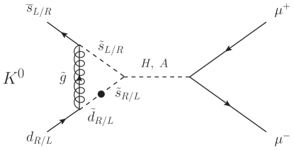
Figure 1: Feynman diagram of the leading (pseudo-)scalar MSSM contributions to $K^{0}_{S}\rightarrow\mu^{+}\mu^{-}$ and $K^{0}_{L}\rightarrow\mu^{+}\mu^{-}$, which include a gluino and a heavy Higgs boson. The black dot is the corresponding mass insertion term.

The leading MSSM contributions to $C_{S(P)}$ and $\tilde{C}_{S(P)}$ in $K^{0}_{S}\rightarrow\mu^{+}\mu^{-}$ and $K^{0}_{L}\rightarrow\mu^{+}\mu^{-}$ are shown in figure 1. For $C_{S}$ and $\tilde{C}_{S}$, we obtain

$${C}_{S}= -\frac{2}{3}\frac{\alpha_{s}\alpha_{2}m_{\mu}}{M_{W}^{2}}\frac{\mu M_{3}}{M_{A}^{2}\tilde{m}_{d}^{2}}\left(\delta^{RR}_{d}\right)_{12}\frac{\tan^{3}\beta}{(1+\epsilon_{g}\tan\beta)^{2}(1+\epsilon_{\ell}\tan\beta)}G\left(x^{3}_{d},x^{Q}_{d}\right)$$

$$-\frac{2}{3}\frac{\alpha_{s}\alpha_{2}m_{\mu}}{M_{W}^{2}}\frac{m_{b}}{m_{s}}\frac{\mu M_{3}\tilde{m}_{Q}^{2}}{M_{A}^{2}\tilde{m}_{d}^{4}}\left(\delta^{RR}_{d}\right)_{13}\left(\delta^{LL}_{d}\right)_{32}$$

$$\leavevmode\nobreak\ \leavevmode\nobreak\ \leavevmode\nobreak\ \leavevmode\nobreak\ \times\frac{\tan^{3}\beta}{(1+\epsilon_{g}\tan\beta)[1+(\epsilon_{g}+\epsilon_{Y}y_{t}^{2})\tan\beta](1+\epsilon_{\ell}\tan\beta)}H\left(x^{3}_{d},x^{Q}_{d}\right),$$ (2.40)

$$\tilde{C}_{S}= -\frac{2}{3}\frac{\alpha_{s}\alpha_{2}m_{\mu}}{M_{W}^{2}}\frac{\mu M_{3}}{M_{A}^{2}\tilde{m}_{Q}^{2}}\left(\delta^{LL}_{d}\right)_{12}\frac{\tan^{3}\beta}{(1+\epsilon_{g}\tan\beta)^{2}(1+\epsilon_{\ell}\tan\beta)}G\left(x^{3}_{Q},x^{d}_{Q}\right)$$

$$-\frac{2}{3}\frac{\alpha_{s}\alpha_{2}m_{\mu}}{M_{W}^{2}}\frac{m_{b}}{m_{s}}\frac{\mu M_{3}\tilde{m}_{d}^{2}}{M_{A}^{2}\tilde{m}_{Q}^{4}}\left(\delta^{LL}_{d}\right)_{13}\left(\delta^{RR}_{d}\right)_{32}$$

$$\leavevmode\nobreak\ \leavevmode\nobreak\ \leavevmode\nobreak\ \leavevmode\nobreak\ \times\frac{\tan^{3}\beta}{(1+\epsilon_{g}\tan\beta)[1+(\epsilon_{g}+\epsilon_{Y}y_{t}^{2})\tan\beta](1+\epsilon_{\ell}\tan\beta)}H\left(x^{3}_{Q},x^{d}_{Q}\right)$$

$$+\frac{(\alpha_{2})^{2}m_{\mu}m_{t}^{2}}{8M_{W}^{4}}\frac{\mu A_{t}}{M_{A}^{2}\tilde{m}_{Q}^{2}}V_{ts}^{\ast}V_{td}\frac{\tan^{3}\beta[1+(\epsilon_{g}+\epsilon_{Y}y_{t}^{2})\tan\beta]^{2}}{(1+\epsilon_{g}\tan\beta)^{4}(1+\epsilon_{\ell}\tan\beta)}F\left(x^{\mu}_{Q},x^{u}_{Q}\right)$$

$$+\frac{(\alpha_{2})^{2}m_{\mu}}{4M_{W}^{2}}\frac{\mu M_{2}}{M_{A}^{2}\tilde{m}_{Q}^{2}}\left(\delta^{LL}_{u}\right)_{12}\frac{\tan^{3}\beta}{(1+\epsilon_{g}\tan\beta)^{2}(1+\epsilon_{\ell}\tan\beta)}G\left(x^{2}_{Q},x^{\mu}_{Q}\right),$$ (2.41)

with

$$\epsilon_{g} =\frac{2\alpha_{s}}{3\pi}\frac{\mu M_{3}}{\tilde{m}_{Q}^{2}}F\left(x^{3}_{Q},x^{d}_{Q}\right),$$ (2.42)

$$\epsilon_{Y} =\frac{1}{16\pi}\frac{\mu A_{t}}{\tilde{m}_{Q}^{2}}F\left(x^{\mu}_{Q},x^{u}_{Q}\right),$$ (2.43)

$$\epsilon_{\ell} \simeq-\frac{3\alpha_{2}}{16\pi},$$ (2.44)

where $x^{3}_{d}=M_{3}^{2}/\tilde{m}_{d}^{2}$, $x^{Q}_{d}=\tilde{m}_{Q}^{2}/\tilde{m}_{d}^{2}$, $x^{3}_{Q}=M_{3}^{2}/\tilde{m}_{Q}^{2}$, $x^{d}_{Q}=\tilde{m}_{d}^{2}/\tilde{m}_{Q}^{2}$, $x^{\mu}_{Q}=\mu^{2}/\tilde{m}_{Q}^{2}$, $x^{u}_{Q}=\tilde{m}_{u}^{2}/\tilde{m}_{Q}^{2}$, $x^{2}_{Q}=M_{2}^{2}/\tilde{m}_{Q}^{2}$, and $x^{\mu}_{Q}=\mu^{2}/\tilde{m}_{Q}^{2}$. The loop functions $F(x,y)$, $G(x,y)$, and $H(x,y)$ are defined in appendix B.1. These results are consistent with ref. Altmannshofer:2009ne in the universal squark mass limit after changing the flavour and its chirality for $B_{s}^{0}$ decay. Here, we used the following approximation

$$\alpha\simeq\beta-\frac{\pi}{2},\quad M_{H}\simeq M_{A},$$ (2.45)

where $\alpha$ is an angle of the orthogonal rotation matrix for the $CP$-even Higgs mass, and $M_{H}$ ($M_{A}$) is a $CP$-even (odd) heavy Higgs mass. On the other hand, the contributions to $C_{P}$ and $\tilde{C}_{P}$ are

$$C_{P}=-C_{S},\quad\tilde{C}_{P}=\tilde{C}_{S}.$$ (2.46)

Note that the Wilson coefficients in the MSSM are given at the $\mu^{\rm SUSY}$ scale, and there is no QCD correction from the renormalization-group (RG) evolution at the leading order.

2.4 $\boldsymbol{\varepsilon^{\prime}_{K}/\varepsilon_{K}}$

New physics models affecting $\varepsilon^{\prime}_{K}/\varepsilon_{K}$ have recently attracted some attention since lattice results from the RBC and UKQCD collaborations Blum:2011ng ; Blum:2012uk ; Blum:2015ywa ; Bai:2015nea have been reported $2$–$3\sigma$ below Buras:2015yba ; Kitahara:2016nld the experimental world average of Re$(\varepsilon^{\prime}_{K}/\varepsilon_{K})$ Patrignani:2016xqp . This is consistent with the recent calculations in the large-$N_{c}$ analyses Buras:2015xba ; Buras:2016fys . Although the lattice simulation Bai:2015nea includes final-state interactions partially along the line of ref. Lellouch:2000pv , final-state interactions have to be still fully included in the calculations in light of a discrepancy of a strong phase shift $\delta_{0}$ Colangelo:2001df ; GarciaMartin:2011cn ; Colangelo:NA62 . Conversely combining large-$N_{c}$ methods with chiral loop corrections can bring the value of $\varepsilon^{\prime}_{K}/\varepsilon_{K}$ in agreement with the experiment Pallante:2001he ; Hambye:2003cy ; Mullor .

In this paper, we used the hadronic matrix elements obtained by lattice simulations. For the $\chi^{2}$ test, we use the following constraint,

$$\Delta\left(\frac{\varepsilon^{\prime}_{K}}{\varepsilon_{K}}\right)^{{\rm EXP}-{\rm SM}}\equiv\textrm{Re}\left(\frac{\varepsilon^{\prime}_{K}}{\varepsilon_{K}}\right)^{\rm EXP}-\left(\frac{\varepsilon^{\prime}_{K}}{\varepsilon_{K}}\right)^{\rm SM}=\left[15.5\pm 2.3\text{(EXP)}\pm 5.07\text{(TH)}\right]\times 10^{-4},$$ (2.47)

with

$$\left(\frac{\varepsilon^{\prime}_{K}}{\varepsilon_{K}}\right)^{\rm SM}\rightarrow\left(\frac{\varepsilon^{\prime}_{K}}{\varepsilon_{K}}\right)^{\rm SM}+\left(\frac{\varepsilon^{\prime}_{K}}{\varepsilon_{K}}\right)^{\rm SUSY},$$ (2.48)

where the SM prediction at the next-to-leading order in ref. Kitahara:2016nld is used. The experimental value of $\varepsilon_{K}$ is used in the calculation of the ratio. The SUSY contributions to $\varepsilon_{K}$ are given in the next subsection.

Within the MSSM, the SUSY contributions to $\varepsilon^{\prime}_{K}/\varepsilon_{K}$ are dominated by gluino box, chargino-mediated $Z$-penguin, and chromomagnetic dipole contributions. The first two contributions are represented by the same $|\Delta S|=1$ four-quark effective Hamiltonian at the $\mu^{\textrm{SUSY}}$ scale, which is:

$$\mathcal{H}_{\rm eff}=\frac{G_{F}}{\sqrt{2}}\sum_{q}\sum_{i=1}^{4}\left[C_{i}^{q}Q_{i}^{q}+\tilde{C}_{i}^{q}\tilde{Q}_{i}^{q}\right]+{\rm H.c.},$$ (2.49)

with

$$Q^{q}_{1}=\left(\bar{s}d\right)_{V-A}\left(\bar{q}q\right)_{V+A},\leavevmode\nobreak\ \leavevmode\nobreak\ \leavevmode\nobreak\ \leavevmode\nobreak\ \leavevmode\nobreak\ \leavevmode\nobreak\ \leavevmode\nobreak\ \leavevmode\nobreak\ \tilde{Q}^{q}_{1}=\left(\bar{s}d\right)_{V+A}\left(\bar{q}q\right)_{V-A},$$

$$Q^{q}_{2}=\left(\bar{s}_{\alpha}d_{\beta}\right)_{V-A}\left(\bar{q}_{\beta}q_{\alpha}\right)_{V+A},\leavevmode\nobreak\ \leavevmode\nobreak\ \tilde{Q}^{q}_{2}=\left(\bar{s}_{\alpha}d_{\beta}\right)_{V+A}\left(\bar{q}_{\beta}q_{\alpha}\right)_{V-A},$$

$$Q^{q}_{3}=\left(\bar{s}d\right)_{V-A}\left(\bar{q}q\right)_{V-A},\leavevmode\nobreak\ \leavevmode\nobreak\ \leavevmode\nobreak\ \leavevmode\nobreak\ \leavevmode\nobreak\ \leavevmode\nobreak\ \leavevmode\nobreak\ \leavevmode\nobreak\ \tilde{Q}^{q}_{3}=\left(\bar{s}d\right)_{V+A}\left(\bar{q}q\right)_{V+A},$$

$$Q^{q}_{4}=\left(\bar{s}_{\alpha}d_{\beta}\right)_{V-A}\left(\bar{q}_{\beta}q_{\alpha}\right)_{V-A},\leavevmode\nobreak\ \leavevmode\nobreak\ \tilde{Q}^{q}_{4}=\left(\bar{s}_{\alpha}d_{\beta}\right)_{V+A}\left(\bar{q}_{\beta}q_{\alpha}\right)_{V+A},$$ (2.50)

where $(V\mp A)$ refers to $\gamma_{\mu}(1\mp\gamma_{5})$, and $\alpha$ and $\beta$ are color indices.

The Wilson coefficients from the gluino box contributions are leading contributions when the mass difference between right-handed squarks exists Kitahara:2016otd ; Kagan:1999iq . They are shown in appendix A.1 with their corresponding loop functions defined in appendix B.2.1. Here, $(\delta_{d})_{13}(\delta_{d})_{32}$ terms are discarded for simplicity.

The Wilson coefficients of the chargino-mediated $Z$-penguin are induced by terms of second order in the expansion of MIA. These ones are shown in appendix A.2, where the loop function $l(x,y)$ is given by eq. (B.1).

The matching conditions to the standard four-quark Wilson coefficients Kitahara:2016nld are

$$\begin{array}[]{ll}s_{1}=0,&s_{2}=0,\\ \\ s_{3}=\frac{1}{3}\left(C_{3}^{u}+2C_{3}^{d}\right),&s_{4}=\frac{1}{3}\left(C_{4}^{u}+2C_{4}^{d}\right),\\ \\ s_{5}=\frac{1}{3}\left(C_{1}^{u}+2C_{1}^{d}\right),&s_{6}=\frac{1}{3}\left(C_{2}^{u}+2C_{2}^{d}\right),\\ \\ s_{7}=\frac{2}{3}\left(C_{1}^{u}-C_{1}^{d}\right),&s_{8}=\frac{2}{3}\left(C_{2}^{u}-C_{2}^{d}\right),\\ \\ s_{9}=\frac{2}{3}\left(C_{3}^{u}-C_{3}^{d}\right),&s_{10}=\frac{2}{3}\left(C_{4}^{u}-C_{4}^{d}\right).\end{array}$$ (2.60)

The coefficients for the opposite-chirality operators, $\tilde{s}_{1,\dots,10}$, are trivially found from the previous ones by replacing ${C}_{1,2,3,4}^{q}\rightarrow\tilde{C}_{1,2,3,4}^{q}$. Using the Wilson coefficients $\vec{s}=(s_{1},s_{2},\dots,s_{10})^{T}$ and $\vec{\tilde{s}}=(\tilde{s}_{1},\tilde{s}_{2},\dots,\tilde{s}_{10})^{T}$ at the $\mu^{\textrm{SUSY}}$ scale, the dominant box and penguin contributions to $\varepsilon^{\prime}_{K}/\varepsilon_{K}$ are given by Kitahara:2016nld

$$\left.\frac{\varepsilon^{\prime}_{K}}{\varepsilon_{K}}\right|_{\textrm{box}+\textrm{pen}} =\frac{G_{F}\omega_{+}}{2|\varepsilon_{K}^{\textrm{EXP}}|\textrm{Re}A_{0}^{\textrm{EXP}}}\langle\vec{Q}_{\varepsilon^{\prime}}(\mu)^{T}\rangle\hat{U}(\mu,\mu^{\textrm{SUSY}})\textrm{Im}\left[\vec{s}-\vec{\tilde{s}}\right],$$ (2.61)

with

$$\omega_{+} =\left(4.53\pm 0.02\right)\times 10^{-2},$$ (2.62)

$$|\varepsilon_{K}^{\textrm{EXP}}| =\left(2.228\pm 0.011\right)\times 10^{-3},$$ (2.63)

$$\textrm{Re}A_{0}^{\textrm{EXP}} =\left(3.3201\pm 0.0018\right)\times 10^{-7}\textrm{\leavevmode\nobreak\ GeV}.$$ (2.64)

The hadronic matrix elements at $\mu=1.3$ GeV, including $I=0$ and $I=2$ parts, are Kitahara:2016nld

$$\langle\vec{Q}_{\varepsilon^{\prime}}(\mu)^{T}\rangle= \Bigl{(}0.345,0.133,0.034,-0.179,0.152,0.288,2.653,17.305,0.526,0.281\Bigr{)}\leavevmode\nobreak\ \textrm{(GeV})^{3},$$ (2.65)

and the approximate function of the RG evolution matrix $\hat{U}(\mu,\mu^{\textrm{SUSY}})$ is given in ref. Kitahara:2016nld .

Next, the $|\Delta S|=1$ chromomagnetic-dipole operator that contributes to $\varepsilon^{\prime}_{K}/\varepsilon_{K}$ is

$$\mathcal{H}_{\textrm{eff}} =C_{g}^{-}Q_{g}^{-}+\textrm{H.c.},$$ (2.66)

with

$$Q_{g}^{-} =-\frac{g_{s}}{(4\pi)^{2}}\left(\overline{s}\sigma^{\mu\nu}T^{A}\gamma_{5}d\right)G^{A}_{\mu\nu}.$$ (2.67)

The complete expression for the Wilson coefficient $C_{g}^{-}$ at the $\mu^{\textrm{SUSY}}$ scale is shown in appendix A.3, where $(\delta_{d})_{13}(\delta_{d})_{32}$ terms are discarded for simplicity. The corresponding loop functions $I(x,y)$, $J(x,y)$, $K(x,y)$, $L(x,y)$, $M_{3}(x)$, and $M_{4}(x)$ are defined in appendix B.2.2.

The chromomagnetic-dipole contribution to $\varepsilon^{\prime}_{K}/\varepsilon_{K}$ is Buras:1999da

$$\left.\frac{\varepsilon^{\prime}_{K}}{\varepsilon_{K}}\right|_{\textrm{chromo}} =\frac{\omega_{+}}{|\varepsilon_{K}^{\textrm{EXP}}|\textrm{Re}A_{0}^{\textrm{EXP}}}\left(1-\hat{\Omega}_{{\rm eff}}\right)\frac{11\sqrt{3}}{64\pi^{2}}\frac{M^{2}_{\pi}M_{K}^{2}}{f_{\pi}(m_{s}+m_{d})}\eta_{s}B_{G}\textrm{Im}C_{g}^{-},$$ (2.68)

where $f_{\pi}=(130.2\pm 1.7)$ MeV Patrignani:2016xqp , and Cirigliano:2003nn ; Cirigliano:2003gt ; Buras:2015yba

$$\hat{\Omega}_{{\rm eff}} =0.148\pm 0.080,$$ (2.69)

$$\eta_{s} =\left[\frac{\alpha_{s}(m_{b})}{\alpha_{s}(1.3\textrm{\,GeV})}\right]^{\frac{2}{25}}\left[\frac{\alpha_{s}(m_{t})}{\alpha_{s}(m_{b})}\right]^{\frac{2}{23}}\left[\frac{\alpha_{s}(\mu^{\textrm{SUSY}})}{\alpha_{s}(m_{t})}\right]^{\frac{2}{21}}.$$ (2.70)

According to refs. Buras:1999da ; Barbieri:1999ax , the hadronic matrix element for the chromomagnetic-dipole operator into two pions, $B_{G}$, is enhanced by $1/N_{c}\cdot M_{K}^{2}/M_{\pi}^{2}$ from the large next-to-leading-order corrections that it receives. Therefore, the leading order in the chiral quark model, $B_{G}=1$, is implausible, and we consider $B_{G}=1\pm 3$ in our analyses.

The other contributions are negligible Kitahara:2016otd . Note that the sub-leading contributions which come from the gluino-mediated photon-penguin and the chargino-mediated $Z$-penguins induced by terms of first order in the expansion of the squark mass matrix, have opposite sign and practically cancel each other Kitahara:2016otd .

Finally, the SUSY contributions to $\varepsilon^{\prime}_{K}/\varepsilon_{K}$ are given as

$$\left(\frac{\varepsilon^{\prime}_{K}}{\varepsilon_{K}}\right)^{\textrm{SUSY}}\simeq\left.\frac{\varepsilon^{\prime}_{K}}{\varepsilon_{K}}\right|_{\textrm{box}+\textrm{pen}}+\left.\frac{\varepsilon^{\prime}_{K}}{\varepsilon_{K}}\right|_{\textrm{chromo}}.$$ (2.71)

Note that we discarded the contributions to $\varepsilon^{\prime}_{K}/\varepsilon_{K}$ from the heavy Higgs exchanges, although they give the strong isospin-violating contribution naturally: the contribution is enhanced by $\tan^{3}\beta$ for only down-type four-fermion scalar operators. These contributions must be proportional to $m_{d}m_{s}$ which cannot be compensated by $\tan^{3}\beta$, so that they should be the higher-order contributions for $\varepsilon^{\prime}_{K}/\varepsilon_{K}$.

2.5 $\boldsymbol{\varepsilon_{K}}$ and $\boldsymbol{\Delta M_{K}}$

Although $\varepsilon_{K}$ is one of the most sensitive quantities to new physics, the SM prediction is still controversial. Especially, the leading short-distance contribution to $\varepsilon_{K}$ in the SM is proportional to $|V_{cb}|^{4}$ (cf., ref. Bailey:2015tba ), whose measured values from inclusive semileptonic $B$ decays ($\overline{B}\to X_{c}\ell^{-}\overline{\nu}$) and from exclusive decays ($\overline{B}\to D^{(\ast)}\ell^{-}\overline{\nu}$ and $\Lambda_{b}\to\Lambda_{c}\ell^{-}\overline{\nu}$) are inconsistent at a $4.1\sigma$ level Amhis:2016xyh ; Jang:2017ieg . A recent discussion about the exclusive $|V_{cb}|$ is given in refs. Bigi:2017njr ; Grinstein:2017nlq ; Bernlochner:2017xyx .

In this paper, for the SM prediction, we use Endo:2017ums

$$\varepsilon_{K}^{\rm SM}=\left(2.12\pm 0.18\right)\times 10^{-3},$$ (2.72)

with

$$\varepsilon_{K}=e^{i\varphi_{\varepsilon}}\varepsilon_{K}^{\textrm{SM}},$$ (2.73)

where $\varphi_{\varepsilon}=\tan^{-1}(2\Delta M_{K}/\Delta\Gamma_{K})=(43.51\pm 0.05)^{\circ}$ Patrignani:2016xqp . This value and the uncertainty are based on the inclusive $|V_{cb}|$ Jang:2017ieg , the Wolfenstein parameters in the angle-only-fit method Bevan:2013kaa , and the long-distance contribution obtained by the lattice simulation Bai:2015nea . Combining the measured value in eq. (2.63), we impose

$$\varepsilon_{K}^{\rm EXP/SM}=1.05\pm 0.10\text{(TH)},$$ (2.74)

on the $\chi^{2}$ test, with

$$\varepsilon_{K}^{\textrm{SM}}\to\varepsilon_{K}^{\textrm{SM}}+\varepsilon_{K}^{\textrm{SUSY}}.$$ (2.75)

Note that we also impose $\textrm{Re}(\varepsilon_{K})>0$ from $\textrm{Re}(\varepsilon_{K})=(1.596\pm 0.013)\times 10^{-3}$ Ambrosino:2006ek .

Within the MSSM, the SUSY contributions to $\varepsilon_{K}$ are dominated by gluino box diagrams. In this paper, however, we will focus on their suppressed region. The crossed and uncrossed gluino-box diagrams give opposite sign contributions and there is a certain cancellation region Crivellin:2010ys ; Kitahara:2016otd , and/or simultaneous mixings of $(\delta_{d}^{LL})$ and $(\delta_{d}^{RR})$ can also produce the cancellation. Therefore, we also consider the sub-dominant contributions which come from Wino and Higgsino boxes. The $|\Delta S|=2$ four-quark effective Hamiltonian at the $\mu^{\rm SUSY}$ scale is Gabbiani:1996hi

$$\mathcal{H}_{\textrm{eff}}=\sum_{i=1}^{5}C_{i}Q_{i}+\sum_{i=1}^{3}\tilde{C}_{i}\tilde{Q}_{i}+\textrm{H.c.},$$ (2.76)

with

$$Q_{1} =\left(\overline{{d}}\gamma_{\mu}P_{L}s\right)\left(\overline{{d}}\gamma^{\mu}P_{L}s\right),\leavevmode\nobreak\ \leavevmode\nobreak\ \leavevmode\nobreak\ Q_{2}=\left(\overline{{d}}P_{L}s\right)\left(\overline{{d}}P_{L}s\right),\leavevmode\nobreak\ \leavevmode\nobreak\ \leavevmode\nobreak\ Q_{3}=\left(\overline{{d}}_{\alpha}P_{L}s_{{\beta}}\right)\left(\overline{{d}}_{\beta}P_{L}s_{{\alpha}}\right),$$

$$Q_{4} =\left(\overline{{d}}P_{L}s\right)\left(\overline{{d}}P_{R}s\right),\leavevmode\nobreak\ \leavevmode\nobreak\ \leavevmode\nobreak\ \leavevmode\nobreak\ \leavevmode\nobreak\ \leavevmode\nobreak\ \leavevmode\nobreak\ \leavevmode\nobreak\ \leavevmode\nobreak\ \,Q_{5}=\left(\overline{{d}}_{\alpha}P_{L}s_{{\beta}}\right)\left(\overline{{d}}_{\beta}P_{R}s_{{\alpha}}\right),$$

$$\tilde{Q}_{1} =\left(\overline{{d}}\gamma_{\mu}P_{R}s\right)\left(\overline{{d}}\gamma^{\mu}P_{R}s\right),\leavevmode\nobreak\ \leavevmode\nobreak\ \leavevmode\nobreak\ \tilde{Q}_{2}=\left(\overline{{d}}P_{R}s\right)\left(\overline{{d}}P_{R}s\right),\leavevmode\nobreak\ \leavevmode\nobreak\ \leavevmode\nobreak\ \tilde{Q}_{3}=\left(\overline{{d}}_{\alpha}P_{R}s_{{\beta}}\right)\left(\overline{{d}}_{\beta}P_{R}s_{{\alpha}}\right).$$ (2.77)

The kaon mixing amplitude $M_{12}^{(K)}$, $\Delta M_{K}$ and $\varepsilon_{K}$ are given by

$$M_{12}^{(K)} =\frac{\langle K^{0}|\mathcal{H}_{\textrm{eff}}|\overline{K}{}^{0}\rangle}{2M_{K}},$$ (2.78)

$$\Delta M_{K} =2\textrm{Re}[M_{12}^{(K)}],$$ (2.79)

$$\varepsilon_{K} =\kappa_{\varepsilon}\frac{e^{i\varphi_{\varepsilon}}}{\sqrt{2}}\frac{\textrm{Im}[M_{12}^{(K)}]}{\Delta M_{K}^{\textrm{EXP}}}=e^{i\varphi_{\varepsilon}}\varepsilon_{K}^{\rm SUSY},$$ (2.80)

where $\kappa_{\varepsilon}=0.94\pm 0.02$ Buras:2010pza . Using the latest lattice result Garron:2016mva , for the hadronic matrix elements, we obtain

$$\langle K^{0}|\vec{Q}(\mu)|\overline{K}{}^{0}\rangle=\Bigl{(}0.00211,-0.04231,0.01288,0.09571,0.02452\Bigr{)}\leavevmode\nobreak\ \textrm{(GeV})^{4},$$ (2.81)

with $\langle K^{0}|\tilde{Q}_{1,2,3}(\mu)|\overline{K}{}^{0}\rangle=\langle K^{0}|Q_{1,2,3}(\mu)|\overline{K}{}^{0}\rangle$, where $\mu=3$ GeV and we used $m_{s}(\mu)=(81.64\pm 1.17)$ MeV and $m_{d}(\mu)=(2.997\pm 0.049)$ MeV Garron:2016mva .

The leading-order QCD RG corrections are given by Bagger:1997gg

$$C_{1}(\mu) =\eta^{K}_{1}C_{1}(\mu^{\rm SUSY}),$$ (2.82)

$$\begin{pmatrix}C_{2}(\mu)\\ C_{3}(\mu)\end{pmatrix} =X_{23}\eta^{K}_{23}X^{-1}_{23}\begin{pmatrix}C_{2}(\mu^{\rm SUSY})\\ C_{3}(\mu^{\rm SUSY})\end{pmatrix},$$ (2.83)

$$\begin{pmatrix}C_{4}(\mu)\\ C_{5}(\mu)\end{pmatrix} =\begin{pmatrix}(\eta^{K}_{1})^{-4}&\frac{1}{3}\left[(\eta^{K}_{1})^{-4}-(\eta^{K}_{1})^{\frac{1}{2}}\right]\\ 0&(\eta^{K}_{1})^{\frac{1}{2}}\end{pmatrix}\begin{pmatrix}C_{4}(\mu^{\rm SUSY})\\ C_{5}(\mu^{\rm SUSY})\end{pmatrix},$$ (2.84)

with

$$\eta^{K}_{1} =\left[\frac{\alpha_{s}(m_{b})}{\alpha_{s}(\mu)}\right]^{\frac{6}{25}}\left[\frac{\alpha_{s}(m_{t})}{\alpha_{s}(m_{b})}\right]^{\frac{6}{23}}\left[\frac{\alpha_{s}(\mu^{\rm SUSY})}{\alpha_{s}(m_{t})}\right]^{\frac{6}{21}},$$ (2.85)

$$\eta^{K}_{23} =\begin{pmatrix}(\eta^{K}_{1})^{\frac{1}{6}\left(1-\sqrt{241}\right)}&0\\ 0&(\eta^{K}_{1})^{\frac{1}{6}\left(1+\sqrt{241}\right)}\end{pmatrix},$$ (2.86)

$$X_{23} =\begin{pmatrix}\frac{1}{2}\left(-15-\sqrt{241}\right)&\frac{1}{2}\left(-15+\sqrt{241}\right)\\ 1&1\end{pmatrix}.$$ (2.87)

The QCD corrections to $\tilde{C}_{1,2,3}$ are the same as ${C}_{1,2,3}$.

The Wilson coefficients from the $|\Delta S|=2$ gluino boxes are shown in appendix A.4 with their corresponding loop functions defined in appendix B.3.1. In the universal squark mass limit, these results are consistent with ref. Altmannshofer:2009ne . Here, the terms proportional to $\left[(\mathcal{M}_{D}^{2})_{LR}\right]_{12}$ or $(\delta_{d})_{13}(\delta_{d})_{32}$ are discarded for simplicity.

The Wilson coefficients and their corresponding loop functions for the sub-leading contributions to $\varepsilon_{K}$ are given in appendix A.5 and B.3.2, respectively.

3 Parameter scan

The MSSM parameter scan is performed with the framework Ipanema-$\beta$ Ipanema using a GPU of the model GeForce GTX 1080. The samples are a combination of flat scans plus scans based on genetic algorithms IEEE . The cost function used by the genetic algorithm is the likelihood function with the observable constrains. In addition, aiming to get a dense population in regions with $\mathcal{B}(K_{S}^{0}\rightarrow\mu^{+}\mu^{-})$ significantly different from the SM prediction, specific penalty contributions are added to the total cost function. We also perform specific scans at $\tan\beta\approx 50$ and $M_{A}\approx 1.6$ TeV as for those values the chances to get sizable MSSM effects are larger.

We study three different scenarios (for the ranges of the scanned parameters see table 2):

• Scenario A: A generic scan with universal gaugino masses. No constraint on the Dark Matter relic density is applied in this case, other than the requirement of neutralino Lightest Supersymmetric Particle (LSP). The LSP is Bino-like in most cases, although some points with Higgsino LSP are also found.

• Scenario B: A scan motivated by scenarios with Higgsino Dark Matter. In this scenario, the relic density is mostly function of the LSP mass, which fulfills the measured density Planck at $m_{\chi_{1}^{0}}\approx 1$ TeV Costa:2017gup ; Bagnaschi:2017tru ; Bagnaschi:2015eha ; Bagnaschi:2016xfg . Thus, we perform a scan with $|\mu|=1$ TeV $<M_{1}$. We assume universal gaugino masses in this scenario, which then implies that $M_{3}>4.5$ TeV.

• Scenario C: A scan motivated by scenarios with Wino Dark Matter, which is possible in mAMSB or pMSSM, although it is under pressure by $\gamma$-rays and antiprotons data Cuoco:2017iax . In those scenarios, the relic density is mostly function of the LSP mass, which fulfills the experimental value Planck at $m_{\chi_{1}^{0}}\approx 3$ TeV Hisano:2006nn ; Bagnaschi:2016xfg . Thus, we make a scan with $M_{2}=3$ TeV $<|\mu|,M_{1,3}$. The Bino mass $M_{1}$ is set to 5 TeV for simplicity. Since it is only necessary in order to ensure that the LSP is Wino-like, any other value above 3 TeV (such as, e.g., an mAMSB-like relation $M_{1}\approx 9.7$ TeV) could also be used without changing the obtained results. The lightest neutralino and the lightest chargino are nearly degenerate, and radiative corrections are expected to bring the chargino mass to be $\approx 160$ MeV heavier than the lightest neutralino Ibe:2012sx .

For simplicity, in all cases we set to zero the trilinear couplings and the mass insertions other than $\left(\delta_{d}^{LL(RR)}\right)_{12}$ and $\left(\delta_{u}^{LL}\right)_{12}$ which is given by the relations in eq. (2.2), and $\mu$ is treated as a real parameter, with both signs allowed a priori.

Parameter	Scenario A	Scenario B	Scenario C
$\tilde{m}_{Q}$	[2, 10]	[2, 10]	[4, 10]
$\tilde{m}_{Q}^{2}/\tilde{m}_{d}^{2}$	[0.25, 4]	[0.25, 4]	[0.25, 4]
$M_{3}$	[2, 10]	[4.5, 15]	[4, 15]
$\tan\beta$	[10, 50]	[10, 50]	[10, 50]
$M_{A}$	[1, 2]	[1, 2]	[1, 2]
$|\mu|$	[1, 10]	$1$	[5, 20]
$M_{1}$	$\frac{\alpha_{1}(\mu^{SUSY})}{\alpha_{3}(\mu^{SUSY})}M_{3}$	$\frac{\alpha_{1}(\mu^{SUSY})}{\alpha_{3}(\mu^{SUSY})}M_{3}$	5
$M_{2}$	$\frac{\alpha_{2}(\mu^{SUSY})}{\alpha_{3}(\mu^{SUSY})}M_{3}$	$\frac{\alpha_{2}(\mu^{SUSY})}{\alpha_{3}(\mu^{SUSY})}M_{3}$	3
$B_{G}$	[-2, 4]	[-2, 4]	[-2, 4]
$\textrm{Re}\left[(\delta_{d}^{LL(RR)})_{12}\right]$	[-0.2, 0.2]	[-0.2, 0.2]	[-0.2, 0.2]
$\textrm{Im}\left[(\delta_{d}^{LL(RR)})_{12}\right]$	[-0.2, 0.2]	[-0.2, 0.2]	[-0.2, 0.2]

Table 2: Scan ranges for scenario A, B (motivated by Higgsino Dark Matter) and C (motivated by Wino Dark Matter). All masses are in TeV. The nuisance parameter $B_{G}$ appears in the chromomagnetic-dipole contribution to $\varepsilon^{\prime}_{K}/\varepsilon_{K}$.

We also perform studies at the MFV limit, using RG equations induced MIs in CMSSM. As expected, no significant effect is found in this case.

For the squark masses, we use $\tilde{m}_{Q}=\tilde{m}_{u}\neq\tilde{m}_{d}$. This set up is motivated by the SUSY $\textrm{SU}(5)$ grand unified theory, where $Q$ and $U$-squark are contained in $\mathbf{10}$ representation matter multiplet while $D$-squark is in $\mathbf{\overline{5}}$ representation one. In general, their soft-SUSY breaking masses are different and depend on couplings between the matter multiplets and the SUSY breaking spurion field.

4 Results

In the following, we show the main results of our scans. The points with $\chi^{2}<12.5$, corresponding to $95\%$ C.L. for six degrees of freedom, are considered experimentally viable. The number of degrees of freedom has been calculated as the number of observables, not counting the nuisance parameter $B_{G}$, the rigid bound on the $\tan\beta$:$M_{A}$ plane, and $\Delta M_{K}$, which are not Gaussian distributed. Therefore, the $\chi^{2}$ requirement corresponds to a $95\%$ C.L. or tighter. Similar plots are obtained if one uses a looser bound on the absolute $\chi^{2}$ accompanied with a $\Delta\chi^{2}<5.99$ across the plane being plotted. Due to the large theory uncertainty, $\mathcal{B}(K_{L}^{0}\rightarrow\mu^{+}\mu^{-})$ can go up to $\approx 1\times 10^{-8}$ at 2$\sigma$ level. Values slightly above that limit can still be allowed if they reduce the $\chi^{2}$ contribution in other observables. The allowed regions are separated by the sign of $A^{\mu}_{L\gamma\gamma}$ in eq. (2.16). We also show results for $A_{CP}$, which could be experimentally accessed by means of a tagged analysis.

4.1 Effects from $\left(\delta_{d}^{LL(RR)}\right)_{12}$ separately

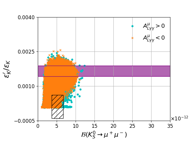
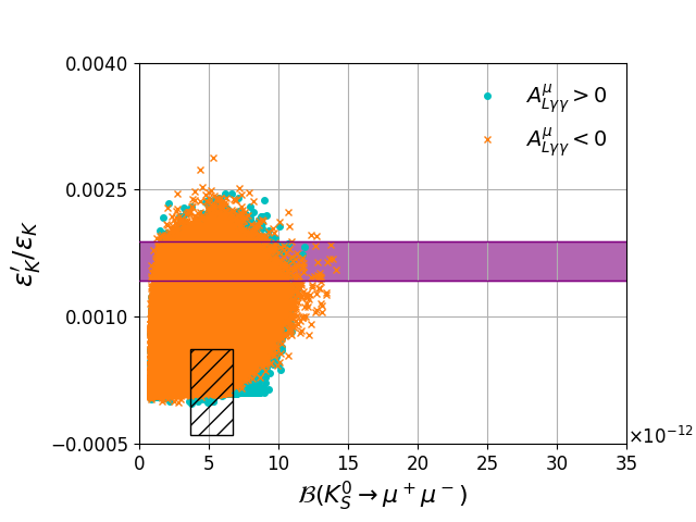
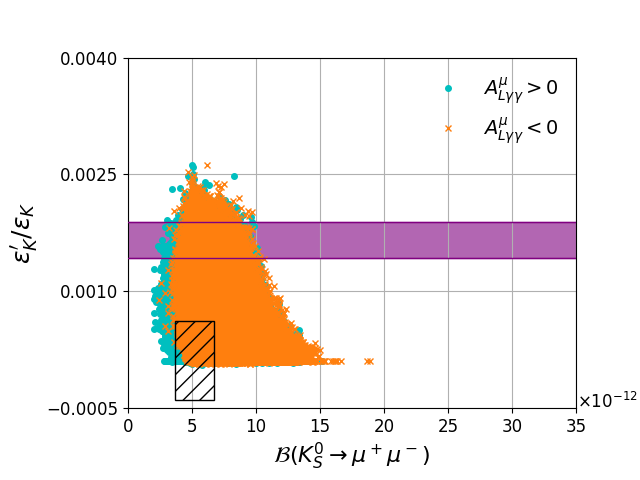
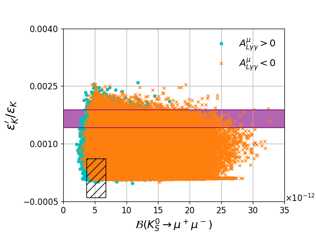
Figure 7: Scenario C, motivated by Wino Dark Matter, $\frac{\varepsilon^{\prime}_{K}}{\varepsilon_{K}}$ vs $\mathcal{B}(K_{S}^{0}\rightarrow\mu^{+}\mu^{-})$ for $\left(\delta_{d}^{LL}\right)_{12}\neq 0$ and $(M_{3}\cdot\mu)>0$ (upper left), $\left(\delta_{d}^{LL}\right)_{12}\neq 0$ and $(M_{3}\cdot\mu)<0$ (upper right), $\left(\delta_{d}^{RR}\right)_{12}\neq 0$ and $(M_{3}\cdot\mu)>0$ (lower left), and $\left(\delta_{d}^{RR}\right)_{12}\neq 0$ and $(M_{3}\cdot\mu)<0$ (lower right). The cyan dots correspond to $A^{\mu}_{L\gamma\gamma}>0$ and the orange crosses to $A^{\mu}_{L\gamma\gamma}<0$. The deep purple band corresponds to the experimental results and the hatched area to the SM prediction.

We first study separately the effects of pure left-handed or pure right-handed MIs, to study the regions of the MSSM parameter space in which either $LL$ MIs or $RR$ MIs dominate. The obtained scatter plots for $\mathcal{B}(K_{L}^{0}\rightarrow\mu^{+}\mu^{-})$ vs $\mathcal{B}(K_{S}^{0}\rightarrow\mu^{+}\mu^{-})$ and $\mathcal{B}(K_{S}^{0}\rightarrow\mu^{+}\mu^{-})$ vs $\varepsilon^{\prime}_{K}/\varepsilon_{K}$ are shown in figure 2 and figure 3 for Scenario A, figure 4 and figure 5 for Scenario B, and figure 6 and figure 7 for Scenario C. The points in the planes correspond to predictions from different values of the input parameters. One should note that in such cases, the SUSY contributions to $\varepsilon_{K}$ can be suppressed naturally in a heavy gluino region ($M_{3}\gtrsim 1.5\tilde{m}_{Q}$) Crivellin:2010ys ; Kitahara:2016otd .

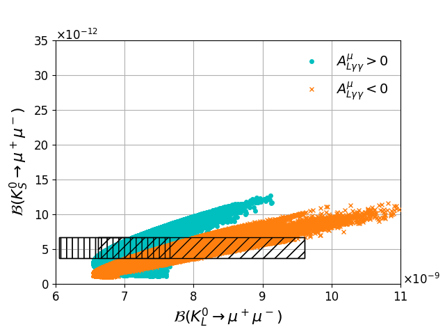
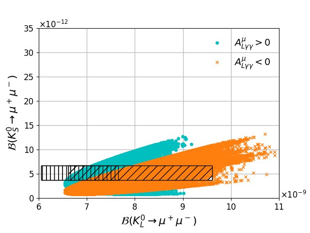
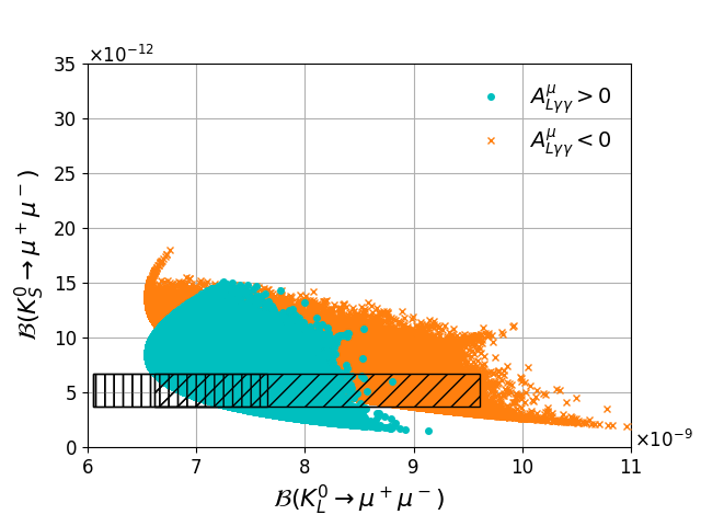
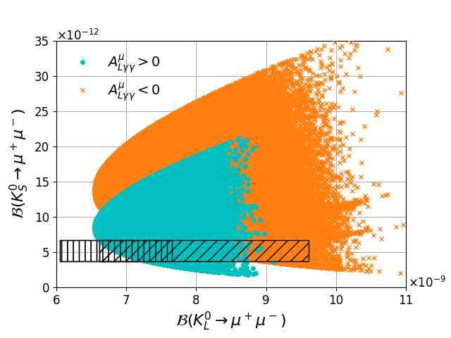
Figure 2: Scenario A $\mathcal{B}(K_{S}^{0}\rightarrow\mu^{+}\mu^{-})$ vs $\mathcal{B}(K_{L}^{0}\rightarrow\mu^{+}\mu^{-})$ for $\left(\delta_{d}^{LL}\right)_{12}\neq 0$ and $(M_{3}\cdot\mu)>0$ (upper left), $\left(\delta_{d}^{LL}\right)_{12}\neq 0$ and $(M_{3}\cdot\mu)<0$ (upper right), $\left(\delta_{d}^{RR}\right)_{12}\neq 0$ and $(M_{3}\cdot\mu)>0$ (lower left), and $\left(\delta_{d}^{RR}\right)_{12}\neq 0$ and $(M_{3}\cdot\mu)<0$ (lower right). The cyan dots correspond to $A^{\mu}_{L\gamma\gamma}>0$ and the orange crosses to $A^{\mu}_{L\gamma\gamma}<0$. The vertically hatched area corresponds to the SM prediction for $A^{\mu}_{L\gamma\gamma}>0$ and the inclined hatched area corresponds to the SM prediction for $A^{\mu}_{L\gamma\gamma}<0$.

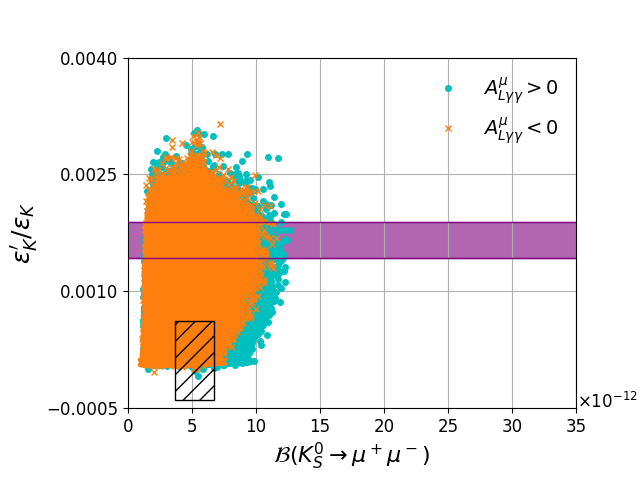
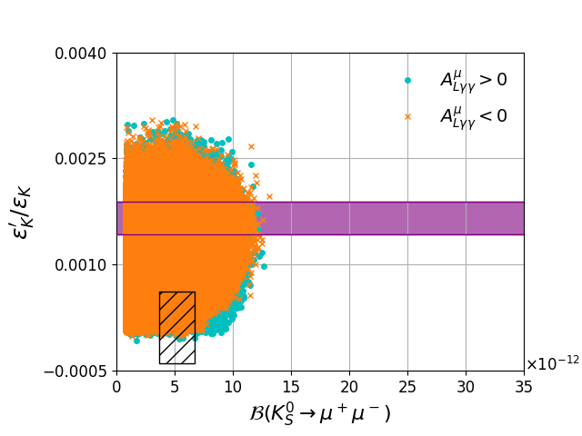
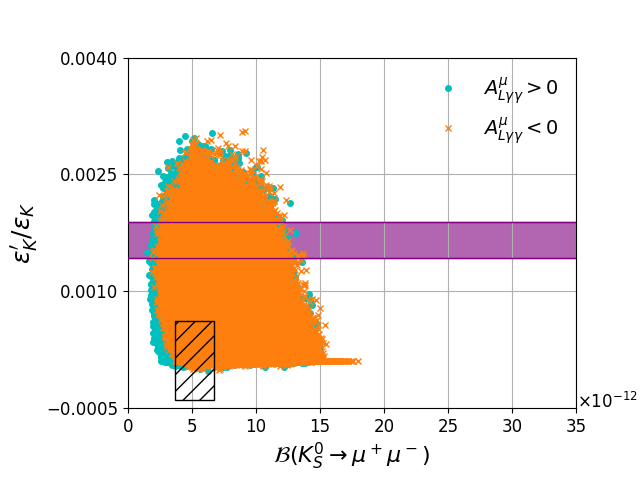
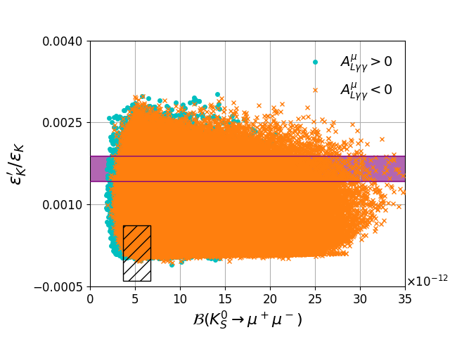
Figure 3: Scenario A $\frac{\varepsilon^{\prime}_{K}}{\varepsilon_{K}}$ vs $\mathcal{B}(K_{S}^{0}\rightarrow\mu^{+}\mu^{-})$ for $\left(\delta_{d}^{LL}\right)_{12}\neq 0$ and $(M_{3}\cdot\mu)>0$ (upper left), $\left(\delta_{d}^{LL}\right)_{12}\neq 0$ and $(M_{3}\cdot\mu)<0$ (upper right), $\left(\delta_{d}^{RR}\right)_{12}\neq 0$ and $(M_{3}\cdot\mu)>0$ (lower left), and $\left(\delta_{d}^{RR}\right)_{12}\neq 0$ and $(M_{3}\cdot\mu)<0$ (lower right). The cyan dots correspond to $A^{\mu}_{L\gamma\gamma}>0$ and the orange crosses to $A^{\mu}_{L\gamma\gamma}<0$. The deep purple band corresponds to the experimental results and the hatched area to the SM prediction.

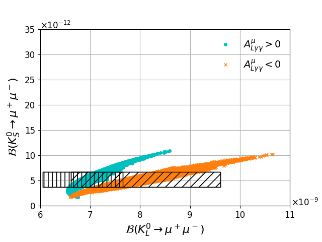
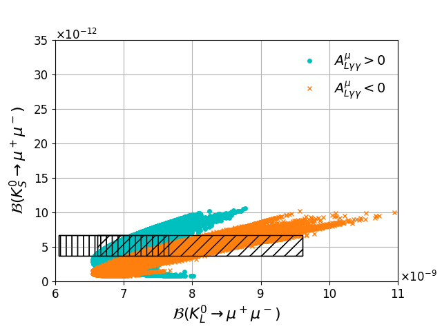
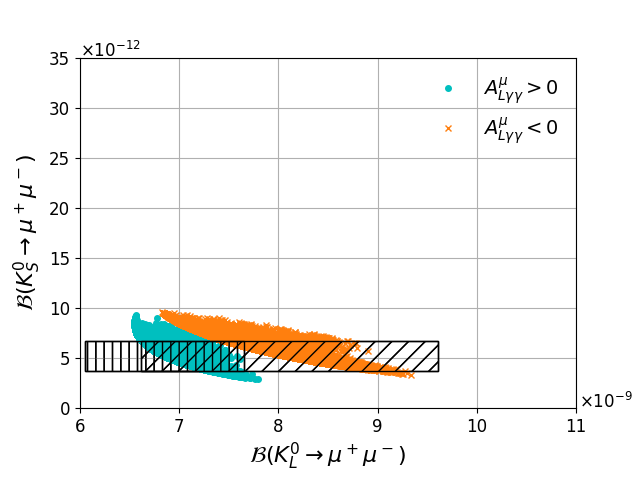
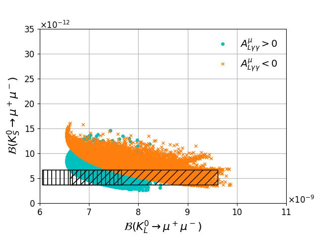
Figure 4: Scenario B, motivated by Higgsino Dark Matter with universal gaugino masses, $\mathcal{B}(K_{S}^{0}\rightarrow\mu^{+}\mu^{-})$ vs $\mathcal{B}(K_{L}^{0}\rightarrow\mu^{+}\mu^{-})$ for $\left(\delta_{d}^{LL}\right)_{12}\neq 0$ and $(M_{3}\cdot\mu)>0$ (upper left), $\left(\delta_{d}^{LL}\right)_{12}\neq 0$ and $(M_{3}\cdot\mu)<0$ (upper right), $\left(\delta_{d}^{RR}\right)_{12}\neq 0$ and $(M_{3}\cdot\mu)>0$ (lower left), and $\left(\delta_{d}^{RR}\right)_{12}\neq 0$ and $(M_{3}\cdot\mu)<0$ (lower right). The cyan dots correspond to $A^{\mu}_{L\gamma\gamma}>0$ and the orange crosses to $A^{\mu}_{L\gamma\gamma}<0$. The vertically hatched area corresponds to the SM prediction for $A^{\mu}_{L\gamma\gamma}>0$ and the inclined hatched area corresponds to the SM prediction for $A^{\mu}_{L\gamma\gamma}<0$.

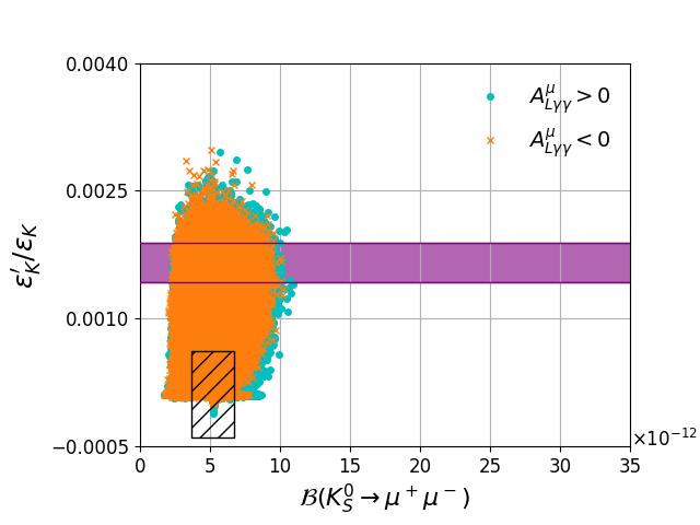
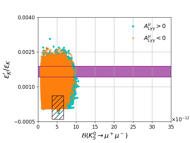
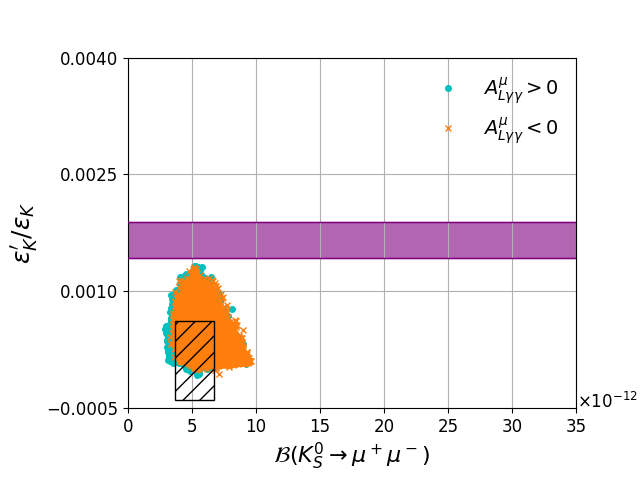
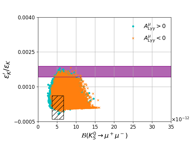
Figure 5: Scenario B, motivated by Higgsino Dark Matter and universal gaugino masses, $\frac{\varepsilon^{\prime}_{K}}{\varepsilon_{K}}$ vs $\mathcal{B}(K_{S}^{0}\rightarrow\mu^{+}\mu^{-})$ for $\left(\delta_{d}^{LL}\right)_{12}\neq 0$ and $(M_{3}\cdot\mu)>0$ (upper left), $\left(\delta_{d}^{LL}\right)_{12}\neq 0$ and $(M_{3}\cdot\mu)<0$ (upper right), $\left(\delta_{d}^{RR}\right)_{12}\neq 0$ and $(M_{3}\cdot\mu)>0$ (lower left), and $\left(\delta_{d}^{RR}\right)_{12}\neq 0$ and $(M_{3}\cdot\mu)<0$ (lower right). The cyan dots correspond to $A^{\mu}_{L\gamma\gamma}<0$ and the orange crosses to $A^{\mu}_{L\gamma\gamma}>0$. The deep purple band corresponds to the experimental results and the hatched area to the SM prediction.

In Scenario A (see figure 2) and Scenario C (see figure 6), we can see that the $95\%$ C.L. allowed regions for $\mathcal{B}(K_{S}^{0}\rightarrow\mu^{+}\mu^{-})$ in light of the constraints listed in table 1 are approximately $[0.78,14]\times 10^{-12}$ for $LL$-only contributions, and $[1.5,35]\times 10^{-12}$ for $RR$-only contributions, without any need of fine-tuning the parameters to avoid constraints from $\mathcal{B}(K_{L}^{0}\rightarrow\mu^{+}\mu^{-})$. The MSSM contributions are similar for $RR$ and $LL$, and the differences on the allowed ranges for $\mathcal{B}(K_{S}^{0}\rightarrow\mu^{+}\mu^{-})$ arise from the interference with the SM amplitudes in $K_{S(L)}^{0}\rightarrow\mu^{+}\mu^{-}$, which are shown in section 2.3. The allowed regions for scenarios A and C are very similar to each other, although marginally larger on A. It can also be seen that, in Scenario B (see figure 4) the maximum departure of $\mathcal{B}(K_{S}^{0}\rightarrow\mu^{+}\mu^{-})$ from the SM is smaller than in the other scenarios, since $C_{S,P}\propto\mu$ and $\mu$ is small relative to squark and gluino masses. In the contributions to $(\varepsilon^{\prime}_{K}/\varepsilon_{K})^{\rm SUSY}$, the chromomagnetic-dipole contribution can be significant in both $LL$-only and $RR$-only cases when $\mu\tan\beta$ and $B_{G}$ have large values, while the box contributions can be significant only via $LL$ MIs Kitahara:2016otd . Note that the penguin contributions to $(\varepsilon^{\prime}_{K}/\varepsilon_{K})^{\rm SUSY}$ are neglected in our parameter scan.

The effective branching fraction and $CP$ asymmetry are shown in figure 8 for Scenario A.Note that the negative value of ${\cal B}(K^{0}_{S}\rightarrow\mu^{+}\mu^{-})_{{\rm eff}}$ is compensated in data by inclusion of the background events from $K^{0}_{L}\rightarrow\mu^{+}\mu^{-}$, so that the overal $K^{0}\rightarrow\mu^{+}\mu^{-}$ is always positive. Correlation patterns of $A_{CP}$ with other observables can be seen in figure 9, where we choose $D^{\prime}=-D$ and $D=0.5$ for simplicity . We find that $CP$ asymmetries can be up to $\approx 6$ (at $D=1$), approximately eight times bigger than in the SM. The largest effects are found in left-handed scenarios.

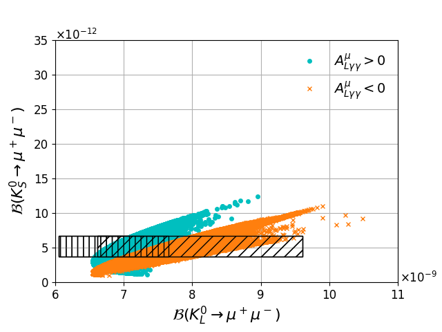
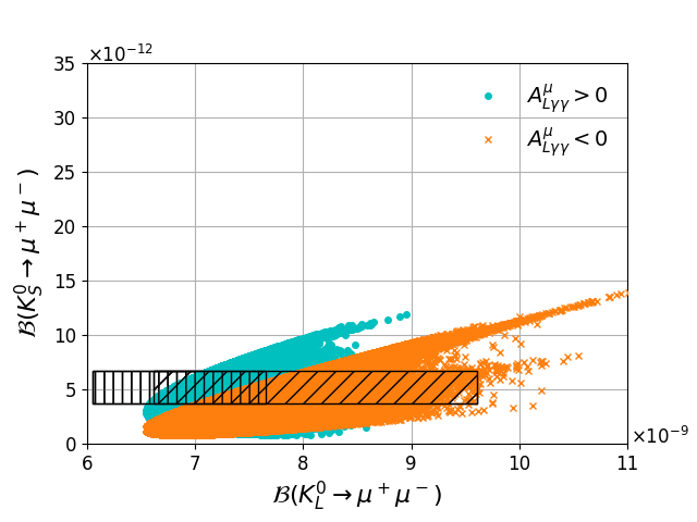
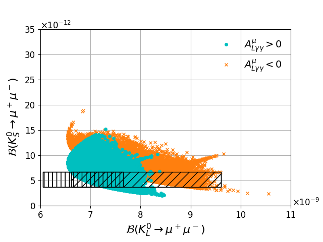
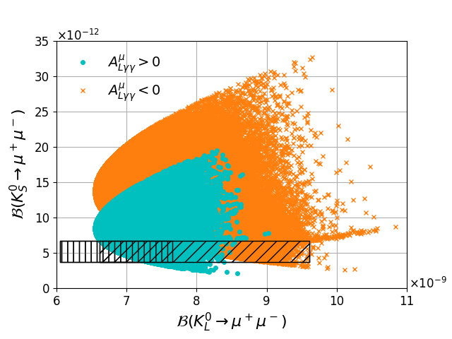
Figure 6: Scenario C (motivated by Wino Dark Matter) $\mathcal{B}(K_{S}^{0}\rightarrow\mu^{+}\mu^{-})$ vs $\mathcal{B}(K_{L}^{0}\rightarrow\mu^{+}\mu^{-})$ for $\left(\delta_{d}^{LL}\right)_{12}\neq 0$ and $(M_{3}\cdot\mu)>0$ (upper left), $\left(\delta_{d}^{LL}\right)_{12}\neq 0$ and $(M_{3}\cdot\mu)<0$ (upper right), $\left(\delta_{d}^{RR}\right)_{12}\neq 0$ and $(M_{3}\cdot\mu)>0$ (lower left), and $\left(\delta_{d}^{RR}\right)_{12}\neq 0$ and $(M_{3}\cdot\mu)<0$ (lower right). The cyan dots correspond to $A^{\mu}_{L\gamma\gamma}>0$ and the orange crosses to $A^{\mu}_{L\gamma\gamma}<0$. The vertically hatched area corresponds to the SM prediction for $A^{\mu}_{L\gamma\gamma}>0$ and the inclined hatched area corresponds to the SM prediction for $A^{\mu}_{L\gamma\gamma}<0$.

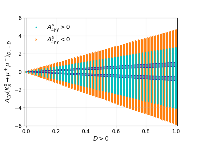
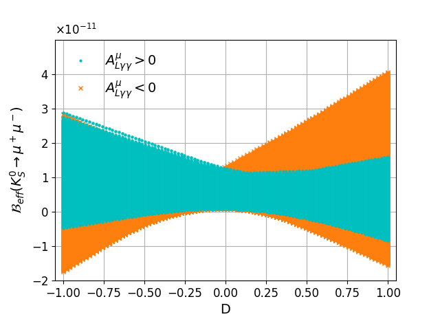
Figure 8: Scenario A, $\left(\delta^{LL}_{d}\right)_{12}\neq 0$ and $(M_{3}\cdot\mu)<0$. Plots of $A_{CP}(K^{0}_{S}\rightarrow\mu^{+}\mu^{-})$ vs $D$ (left) for the case $D=-D^{\prime}$ ($D>0$) where the cyan dots correspond to $A^{\mu}_{L\gamma\gamma}>0$, the orange crosses to $A^{\mu}_{L\gamma\gamma}<0$, and the deep purple bands correspond to the SM predictions in eq. (2.37). ${\cal B}(K^{0}_{S}\rightarrow\mu^{+}\mu^{-})_{{\rm eff}}$ vs $D$ (right).

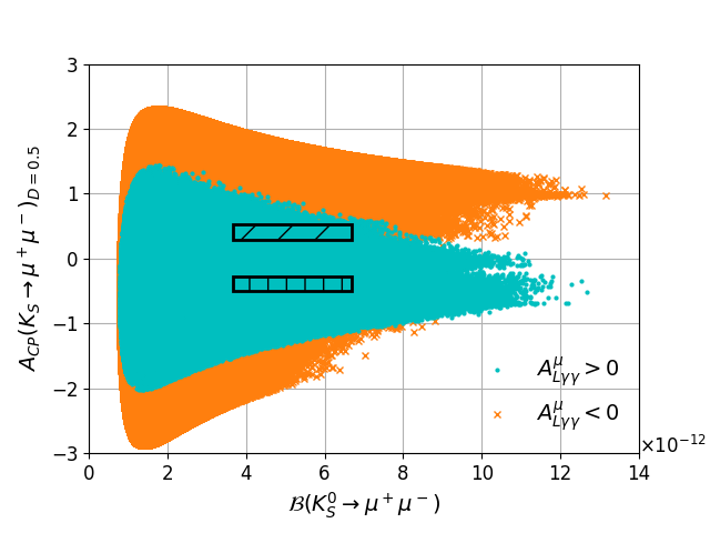
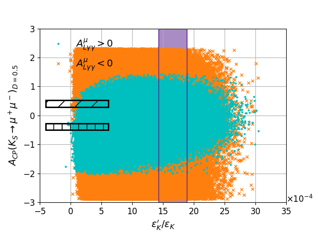
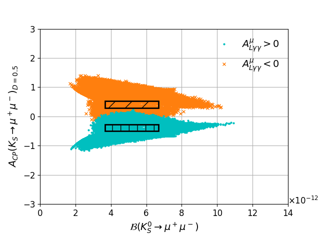
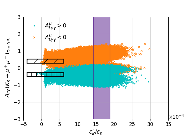
Figure 9: $A_{CP}$ vs $\mathcal{B}(K^{0}_{S}\rightarrow\mu^{+}\mu^{-})$ (left) and vs $\varepsilon^{\prime}_{K}/\varepsilon_{K}$ (right). The top panels correspond to Scenario A, $\left(\delta_{d}^{LL}\right)_{12}\neq 0$ and $(M_{3}\cdot\mu)<0$. The bottom panels correspond to Scenario B, $\left(\delta^{LL}_{d}\right)_{12}\neq 0$ and $(M_{3}\cdot\mu)>0$. The plots are done for $D=-D^{\prime}=0.5$ . The cyan dots correspond to $A^{\mu}_{L\gamma\gamma}>0$ and the orange crosses to $A^{\mu}_{L\gamma\gamma}<0$. The deep purple bands correspond to the experimental value of $\varepsilon^{\prime}_{K}/\varepsilon_{K}$, the vertically hatched areas correspond to the SM prediction for $A^{\mu}_{L\gamma\gamma}>0$ and the inclined hatched areas to the SM prediction for $A^{\mu}_{L\gamma\gamma}<0$ .

4.2 Floating $LL$ and $RR$ MIs simultaneously

A priori, one possibility to avoid the constraint from $\mathcal{B}(K_{L}^{0}\rightarrow\mu^{+}\mu^{-})$ is to allow simultaneously for non-zero $LL$ and $RR$ mass insertions. This way both $C_{S(P)}$ and $\tilde{C}_{S(P)}$ are non zero and eqs. (2.3)–(2.24) do not hold. One can then find regions in which the MSSM contributions to $\mathcal{B}(K_{S}^{0}\rightarrow\mu^{+}\mu^{-})$ do not alter $\mathcal{B}(K_{L}^{0}\rightarrow\mu^{+}\mu^{-})$ significantly.

For instance, if one chooses

$$\textrm{Re}\left[\left(\delta_{d}^{LL}\right)_{12}\right]=-\textrm{Re}\left[\left(\delta_{d}^{RR}\right)_{12}\right],\quad\textrm{Im}\left[\left(\delta_{d}^{LL}\right)_{12}\right]=\textrm{Im}\left[\left(\delta_{d}^{RR}\right)_{12}\right],$$ (4.1)

then the SUSY contributions to $\mathcal{B}(K_{L}^{0}\rightarrow\mu^{+}\mu^{-})$ are canceled, while the SUSY contributions to $\mathcal{B}(K_{S}^{0}\rightarrow\mu^{+}\mu^{-})$ are maximized (see eqs. (2.9)–(2.13)). However, it is known that in those cases the bounds from $\Delta M_{K}$ and $\varepsilon_{K}$ are very stringent. Using genetic algorithms with cost functions that target large values of $\mathcal{B}(K_{S}^{0}\rightarrow\mu^{+}\mu^{-})$, we find fine-tuned regions with $\mathcal{B}(K_{S}^{0}\rightarrow\mu^{+}\mu^{-})>10^{-10}$, or even at the level of the current experimental bound of $8\times 10^{-10}$ at $90\%$ C.L. LHCb:KsMuMu , which are consistent with all our constraints. These points are located along very narrow strips in the $\left(\delta_{d}^{LL}\right)_{12}$ vs $\left(\delta_{d}^{RR}\right)_{12}$ planes, as shown in figure 10. The figure corresponds to Scenario C as it is the one with higher density of points at large values of $\mathcal{B}(K_{S}^{0}\rightarrow\mu^{+}\mu^{-})$ and the pattern observed in Scenario A is nearly identical. A particularly favorable region corresponds to $|(\delta_{d}^{LL})_{12}|\approx 2|(\delta_{d}^{RR})_{12}|\sim 0.03$ and $arg\left[(\delta_{d}^{LL})_{12}\right]\approx-arg\left[(\delta_{d}^{RR})_{12}\right]+\pi$, which is in the vicinity of eq. (4.1), and with $\delta_{u}^{LL}$ given by the symmetry relation of eq. (2.2). They also favor narrow regions in the squark vs gluino masses planes as shown in figure 11. We checked that the values close to the experimental upper bound can still be obtained even if the constraint on $\Delta M_{K}$ is significantly tightened.

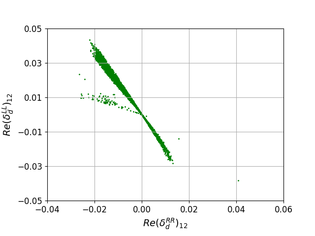
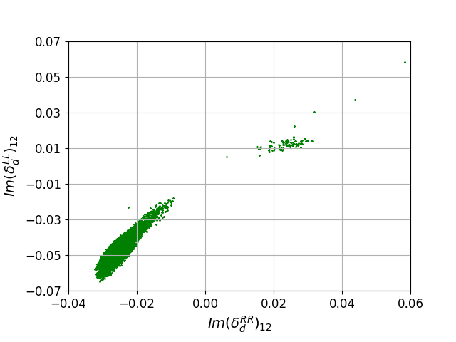
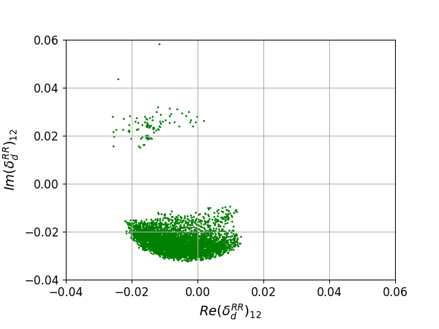
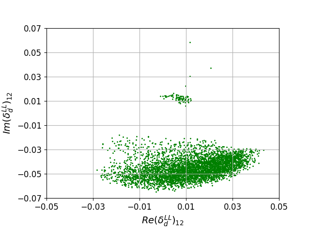
Figure 10: Scatter plots of the real (upper left) and the imaginary (upper right) parts of the mass insertions $\left(\delta_{d}^{RR}\right)_{12}$ and $\left(\delta_{d}^{LL}\right)_{12}$ for $\mathcal{B}(K_{S}^{0}\rightarrow\mu^{+}\mu^{-})>2\times 10^{-10}$, of the real vs imaginary $\left(\delta_{d}^{RR}\right)_{12}$ (lower left) and of the real vs imaginary $\left(\delta_{d}^{LL}\right)_{12}$ (lower right). All points in the plane pass the experimental constraints defined in section 2. The up-type MI $(\delta_{u}^{LL})_{12}$ is given by eq. (2.2). The plots correspond to Scenario C, with a sample of 4378 points with $\mathcal{B}(K_{S}^{0}\rightarrow\mu^{+}\mu^{-})>2\times 10^{-10}$ and $\chi^{2}<12.5$, produced after 6M generations of $200k$ points each. The pattern observed in Scenario A is very similar.

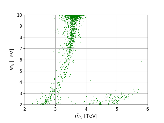
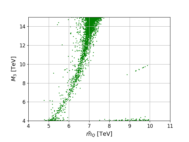
Figure 11: Scatter plot of the squark and gluino masses for $\mathcal{B}(K_{S}^{0}\rightarrow\mu^{+}\mu^{-})>2\times 10^{-10}$ taking into account the constraints defined in section 2. Left: Scenario A, Right: Scenario C. The $\chi^{2}$ cut in Scenario A has been relaxed to $14$ to increase the density of points.

We note that the authors in ref. Jang:2017ieg provide a SM prediction for $\varepsilon_{K}$ less consistent with data than the one we used. That prediction is obtained using $|V_{cb}|$ from exclusive decays. If we use that value instead of eq. (2.74),

$$\varepsilon_{K}^{\rm EXP/SM}=1.41\pm 0.16\text{(TH)},$$ (4.2)

then we can accommodate more easily $LL$ and $RR$ MIs of similar sizes, and fine-tuned regions with $\mathcal{B}(K_{S}^{0}\rightarrow\mu^{+}\mu^{-})>10^{-10}$ are found with higher chances. The shapes of the strips in the mass insertion planes do not change substantially.

4.3 Non degenerate Higgs masses

The results so far have been obtained in the MSSM framework, in which $|C_{S}|\approx|C_{P}|$. This is due to the mass degeneracy $M_{H}\approx M_{A}$. In models in which such degeneracy can be broken, the constraint that $\mathcal{B}(K_{L}^{0}\rightarrow\mu^{+}\mu^{-})$ imposes to $\mathcal{B}(K_{S}^{0}\rightarrow\mu^{+}\mu^{-})$ relaxes the more those two masses differ. This degeneracy is broken in MSSM at low values of $M_{A}$, and requiring $\tan\beta$ to be small to avoid constraints from $\tan\beta:M_{A}$ planes from LHC. Those regions are more difficult to study, since it would require a detailed specification of the MSSM and test it against bounds of the Higgs sector. The mass degeneracy is also broken in extensions such as NMSSM. According to our scans, on those cases one could, in principle, reach values of $\mathcal{B}(K_{S}^{0}\rightarrow\mu^{+}\mu^{-})>10^{-10}$ for mass differences of ${\cal O}(33\%)$ or larger without fine-tuning the MIs.

5 Conclusions

We explored MSSM contribution to $\mathcal{B}(K_{S}^{0}\rightarrow\mu^{+}\mu^{-})$ for non-zero $(\delta_{d}^{LL})_{12}$ and $(\delta_{d}^{RR})_{12}$ mass insertions, motivated by the experimental value of $\varepsilon^{\prime}_{K}/\varepsilon_{K}$, and in the large $\tan{\beta}$ regime. The expressions for the relevant MSSM amplitudes have been provided. We find that MSSM contributions to $\mathcal{B}(K_{S}^{0}\rightarrow\mu^{+}\mu^{-})$ can surpass the SM contributions [$\mathcal{B}(K_{S}^{0}\rightarrow\mu^{+}\mu^{-})^{\textrm{SM}}=5.18\times 10^{-12}$] by up to a factor of seven (see figure 2), reaching the level of $3.5\times 10^{-11}$ even for large SUSY masses, with no conflict with existing experimental data, and are detectable by LHCb. This is also the case even if $\varepsilon^{\prime}_{K}/\varepsilon_{K}$ turns out to be SM-like as predicted by refs. Pallante:2001he ; Hambye:2003cy ; Mullor . Figures of correlations between $\mathcal{B}(K_{S}^{0}\rightarrow\mu^{+}\mu^{-})$ and other observables have been provided for different regions of the MSSM parameter space, and can be used to understand which scenarios are more or less favoured, depending on the experimental outcomes. The $3.5\times 10^{-11}$ bound is due to the combined effect of $\Delta M_{K},\varepsilon_{K}$ , and $K^{0}_{L}\rightarrow\mu^{+}\mu^{-}$ constraints. Such bound is not rigid, and fine-tuned regions can bring the branching fraction above the $10^{-10}$ level, even up to the current experimental bound; the largest deviations from SM are found at $|(\delta_{d}^{LL})_{12}|\approx 2|(\delta_{d}^{RR})_{12}|\sim 0.03$ and $arg\left[(\delta_{d}^{LL})_{12}\right]\approx-arg\left[(\delta_{d}^{RR})_{12}\right]+\pi$ for large squark and gluino masses. We also find that the $CP$ asymmetry of $K^{0}\rightarrow\mu^{+}\mu^{-}$ can be significantly modified by MSSM contributions, being up to eight times bigger than the SM prediction in the pure LL case. Finally, we remind that, for simplicity, we have restricted our study to the main contributions in the large $\tan\beta$ regime. Discarded terms could, in principle, provide even more flexibility to the allowed regions.

Appendix A Wilson coefficients

A.1 $\boldsymbol{|\Delta S|=1}$ gluino box contribution

The Wilson coefficients of the gluino box contributions to $\varepsilon^{\prime}_{K}/\varepsilon_{K}$ are

$$C_{1}^{q} =\frac{(\alpha_{s})^{2}}{2\sqrt{2}G_{F}M_{3}^{2}}\left(\delta_{d}^{LL}\right)_{12}\left[\frac{1}{18}f\left(x^{Q}_{3},x^{q}_{3}\right)-\frac{5}{18}g\left(x^{Q}_{3},x^{q}_{3}\right)\right],$$

$$C_{2}^{q} =\frac{(\alpha_{s})^{2}}{2\sqrt{2}G_{F}M_{3}^{2}}\left(\delta_{d}^{LL}\right)_{12}\left[\frac{7}{6}f\left(x^{Q}_{3},x^{q}_{3}\right)+\frac{1}{6}g\left(x^{Q}_{3},x^{q}_{3}\right)\right],$$

$$C_{3}^{q} =\frac{(\alpha_{s})^{2}}{2\sqrt{2}G_{F}M_{3}^{2}}\left(\delta_{d}^{LL}\right)_{12}\left[-\frac{5}{9}f\left(x^{Q}_{3},x^{Q}_{3}\right)+\frac{1}{36}g\left(x^{Q}_{3},x^{Q}_{3}\right)\right],$$

$$C_{4}^{q} =\frac{(\alpha_{s})^{2}}{2\sqrt{2}G_{F}M_{3}^{2}}\left(\delta_{d}^{LL}\right)_{12}\left[\frac{1}{3}f\left(x^{Q}_{3},x^{Q}_{3}\right)+\frac{7}{12}g\left(x^{Q}_{3},x^{Q}_{3}\right)\right],$$

$$\tilde{C}_{1}^{q} =\frac{(\alpha_{s})^{2}}{2\sqrt{2}G_{F}M_{3}^{2}}\left(\delta_{d}^{RR}\right)_{12}\left[\frac{1}{18}f\left(x^{d}_{3},x^{Q}_{3}\right)-\frac{5}{18}g\left(x^{d}_{3},x^{Q}_{3}\right)\right],$$

$$\tilde{C}_{2}^{q} =\frac{(\alpha_{s})^{2}}{2\sqrt{2}G_{F}M_{3}^{2}}\left(\delta_{d}^{RR}\right)_{12}\left[\frac{7}{6}f\left(x^{d}_{3},x^{Q}_{3}\right)+\frac{1}{6}g\left(x^{d}_{3},x^{Q}_{3}\right)\right],$$

$$\tilde{C}_{3}^{q} =\frac{(\alpha_{s})^{2}}{2\sqrt{2}G_{F}M_{3}^{2}}\left(\delta_{d}^{RR}\right)_{12}\left[-\frac{5}{9}f\left(x^{d}_{3},x^{q}_{3}\right)+\frac{1}{36}g\left(x^{d}_{3},x^{q}_{3}\right)\right],$$

$$\tilde{C}_{4}^{q} =\frac{(\alpha_{s})^{2}}{2\sqrt{2}G_{F}M_{3}^{2}}\left(\delta_{d}^{RR}\right)_{12}\left[\frac{1}{3}f\left(x^{d}_{3},x^{q}_{3}\right)+\frac{7}{12}g\left(x^{d}_{3},x^{q}_{3}\right)\right],$$ (A.1)

where $q$ runs $u$ and $d$, and $x^{Q}_{3}=\tilde{m}_{Q}^{2}/M_{3}^{2}$ and $x^{q}_{3}=\tilde{m}_{q}^{2}/M_{3}^{2}$.

A.2 $\boldsymbol{|\Delta S|=1}$ chargino-mediated $\boldsymbol{Z}$-penguin contribution

The Wilson coefficients of the chargino-mediated $Z$-penguin are

$$C_{1}^{u} =-\frac{(\alpha_{2})^{2}\sin^{2}\theta_{W}}{12\sqrt{2}G_{F}M_{W}^{2}}\frac{\left[(\mathcal{M}_{U}^{2})_{LR}\right]^{\ast}_{23}\left[(\mathcal{M}_{U}^{2})_{LR}\right]_{13}}{M_{2}^{4}}l\left(x^{Q}_{2},x^{u}_{2}\right),$$

$$C_{1}^{d} =\frac{(\alpha_{2})^{2}\sin^{2}\theta_{W}}{24\sqrt{2}G_{F}M_{W}^{2}}\frac{\left[(\mathcal{M}_{U}^{2})_{LR}\right]^{\ast}_{23}\left[(\mathcal{M}_{U}^{2})_{LR}\right]_{13}}{M_{2}^{4}}l\left(x^{Q}_{2},x^{u}_{2}\right),$$

$$C_{3}^{u} =\frac{(\alpha_{2})^{2}}{16\sqrt{2}G_{F}M_{W}^{2}}\left(1-\frac{4}{3}\sin^{2}\theta_{W}\right)\frac{\left[(\mathcal{M}_{U}^{2})_{LR}\right]^{\ast}_{23}\left[(\mathcal{M}_{U}^{2})_{LR}\right]_{13}}{M_{2}^{4}}l\left(x^{Q}_{2},x^{u}_{2}\right),$$

$$C_{3}^{d} =-\frac{(\alpha_{2})^{2}}{16\sqrt{2}G_{F}M_{W}^{2}}\left(1-\frac{2}{3}\sin^{2}\theta_{W}\right)\frac{\left[(\mathcal{M}_{U}^{2})_{LR}\right]^{\ast}_{23}\left[(\mathcal{M}_{U}^{2})_{LR}\right]_{13}}{M_{2}^{4}}l\left(x^{Q}_{2},x^{u}_{2}\right),$$

$$C_{2,4}^{q} =\tilde{C}_{1,2,3,4}^{q}=0.$$ (A.2)

A.3 $\boldsymbol{|\Delta S|=1}$ chromomagnetic dipole contribution

The Wilson coefficients of the chromomagnetic dipole contributions to $\varepsilon^{\prime}_{K}/\varepsilon_{K}$ are

$$C_{g}^{-} =\frac{\alpha_{s}\pi}{3}\frac{\tilde{m}_{Q}^{2}\mu m_{s}}{M_{3}^{5}}\left(\delta_{d}^{LL}\right)_{12}\frac{\tan\beta}{1+\epsilon_{g}\tan\beta}\left[I\left(x^{Q}_{3},x^{d}_{3}\right)+9J\left(x^{Q}_{3},x^{d}_{3}\right)\right]$$

$$-\frac{\alpha_{s}\pi}{3}\frac{\tilde{m}_{d}^{2}\mu m_{s}}{M_{3}^{5}}\left(\delta_{d}^{RR}\right)_{12}\frac{\tan\beta}{1+\epsilon_{g}\tan\beta}\left[I\left(x^{d}_{3},x^{Q}_{3}\right)+9J\left(x^{d}_{3},x^{Q}_{3}\right)\right]$$

$$+\frac{\alpha_{s}\pi}{3}\frac{\left[(\mathcal{M}_{D}^{2})_{LR}\right]_{12}-\left[(\mathcal{M}_{D}^{2})_{LR}\right]^{\ast}_{21}}{M_{3}^{3}}\left[K\left(x^{Q}_{3},x^{d}_{3}\right)+9L\left(x^{Q}_{3},x^{d}_{3}\right)\right]$$

$$-\frac{\alpha_{s}\pi}{3}\frac{m_{s}}{\tilde{m}_{Q}^{2}}\left(\delta_{d}^{LL}\right)_{12}\left[M_{3}\left(x^{3}_{Q}\right)+9M_{4}\left(x^{3}_{Q}\right)\right]$$

$$+\frac{\alpha_{s}\pi}{3}\frac{m_{s}}{\tilde{m}_{d}^{2}}\left(\delta_{d}^{RR}\right)_{12}\left[M_{3}\left(x^{3}_{d}\right)+9M_{4}\left(x^{3}_{d}\right)\right].$$ (A.3)

A.4 $\boldsymbol{|\Delta S|=2}$ gluino box contribution

The Wilson coefficients of the gluino box contributions to $\varepsilon_{K}$ are

$$C_{1} =-\frac{(\alpha_{s})^{2}}{\tilde{m}_{Q}^{2}}\left[\left(\delta^{LL}_{d}\right)_{21}\right]^{2}g^{(1)}_{1}\left(x^{3}_{Q}\right),$$ (A.4)

$$C_{4} =-\frac{(\alpha_{s})^{2}}{M_{3}^{2}}\left[\left(\delta^{LL}_{d}\right)_{21}\left(\delta^{RR}_{d}\right)_{21}\right]g^{(1)}_{4}\left(x^{3}_{Q},x^{3}_{d}\right),$$ (A.5)

$$C_{5} \simeq-\frac{(\alpha_{s})^{2}}{M_{3}^{2}}\left[\left(\delta^{LL}_{d}\right)_{21}\left(\delta^{RR}_{d}\right)_{21}\right]g^{(1)}_{5}\left(x^{3}_{Q},x^{3}_{d}\right),$$ (A.6)

$$\tilde{C}_{1} =-\frac{(\alpha_{s})^{2}}{\tilde{m}_{d}^{2}}\left[\left(\delta^{RR}_{d}\right)_{21}\right]^{2}g^{(1)}_{1}\left(x^{3}_{d}\right),$$ (A.7)

$$C_{2} =C_{3}=\tilde{C}_{2}=\tilde{C}_{3}=0.$$ (A.8)

A.5 Sub-leading contributions to $\boldsymbol{\varepsilon_{K}}$

The Wilson coefficients of the Wino and Higgsino contributions are

$$C_{1} =-\frac{\alpha_{s}\alpha_{2}}{6\tilde{m}_{Q}^{2}}\left[\left(\delta^{LL}_{d}\right)_{21}\right]^{2}g^{(1)}_{\tilde{g}\tilde{w}}\left(x^{3}_{Q},x^{2}_{Q}\right)-\frac{(\alpha_{2})^{2}}{8\tilde{m}_{Q}^{2}}\left[\left(\delta^{LL}_{d}\right)_{21}\right]^{2}g^{(1)}_{\tilde{w}}\left(x^{2}_{Q}\right)$$

$$-\frac{(\alpha_{2})^{2}}{8\tilde{m}_{u}^{2}}\left(V_{ts}V_{td}^{\ast}\right)^{2}\frac{m_{t}^{4}}{M_{W}^{4}}f_{1}\left(x^{\mu}_{u}\right),$$ (A.9)

$$\tilde{C}_{3} =-\frac{(\alpha_{2})^{2}}{8}\left(V_{ts}V_{td}^{\ast}\right)^{2}\frac{m_{s}^{2}\tan^{2}\beta}{(1+\epsilon_{g}\tan\beta)^{2}}\frac{m_{t}^{4}}{M_{W}^{4}}\frac{\mu^{2}A_{t}^{2}}{\tilde{m}_{Q}^{4}\tilde{m}_{u}^{4}}f_{3}\left(x^{\mu}_{Q},x^{\mu}_{u}\right),$$ (A.10)

$$C_{2} =C_{3}=C_{4}=C_{5}=\tilde{C}_{1}=\tilde{C}_{2}=0.$$ (A.11)

Note that a $\tan^{4}\beta$ enhanced contribution to $\varepsilon_{K}$ comes from the exchange of neutral Higgses, which is discarded because of $\left(\delta_{d}\right)_{23}\left(\delta_{d}\right)_{31}=0$ in our analyses. For the Wilson coefficient, we obtain

$$C_{2} \simeq\tilde{C}_{2}\simeq 0,$$ (A.12)

$$C_{4} \simeq-\frac{8(\alpha_{s})^{2}\alpha_{2}}{9\pi}\frac{m_{b}^{2}}{M_{W}^{2}}\frac{\tan^{4}\beta}{(1+\epsilon_{g}\tan\beta)^{2}[1+(\epsilon_{g}+\epsilon_{Y}y_{t}^{2})\tan\beta]^{2}}\frac{\mu^{2}M_{3}^{2}}{M_{A}^{2}\tilde{m}_{Q}^{2}\tilde{m}_{d}^{2}}$$

$$\times\left[\left(\delta^{LL}_{d}\right)_{23}\left(\delta^{LL}_{d}\right)_{31}\left(\delta^{RR}_{d}\right)_{23}\left(\delta^{RR}_{d}\right)_{31}\right]H\left(x^{3}_{Q},x^{d}_{Q}\right)H\left(x^{3}_{d},x^{Q}_{d}\right),$$ (A.13)

$$C_{1} =C_{3}=C_{5}=\tilde{C}_{1}=\tilde{C}_{3}=0,$$ (A.14)

where the approximation in eq. (2.45) is used, and the loop function $H(x,y)$ is given in eq. (B.4). Note that the $CP$-even and $CP$-odd Higgs contributions to $C_{2}$ ($\tilde{C}_{2}$) are canceled out by each other.

Appendix B Loop functions

B.1 $\boldsymbol{K^{0}\rightarrow\mu^{+}\mu^{-}}$

The loop functions $l(x,y)$, $F(x,y)$, $G(x,y)$, and $H(x,y)$ are given by

$$l(x,y) =-\frac{\left[x^{2}+(x-2)y\right]x\ln x}{(x-1)^{2}(x-y)^{3}}+\frac{\left[y^{2}+(y-2)x\right]y\ln y}{(y-1)^{2}(x-y)^{3}}-\frac{x+y-2xy}{(x-1)(y-1)(x-y)^{2}},$$ (B.1)

$$F(x,y) =\frac{x\ln x}{(x-1)(x-y)}+\frac{y\ln y}{(y-1)(y-x)},$$ (B.2)

$$G(x,y) =\frac{x\ln x}{(x-1)^{2}(x-y)}+\frac{y\ln y}{(y-1)^{2}(y-x)}+\frac{1}{(x-1)(y-1)},$$ (B.3)

$$H(x,y) =\frac{x\ln x}{(x-1)^{2}(x-y)^{2}}+\frac{(x+xy-2y^{2})\ln y}{(y-1)^{3}(x-y)^{2}}-\frac{2x-y-1}{(x-1)(y-1)^{2}(x-y)},$$ (B.4)

where $l(1,1)=-1/12$, $F(1,1)=1/2$, $G(1,1)=-1/6$, and $H(1,1)=1/12$.

B.2 $\boldsymbol{\varepsilon^{\prime}_{K}/\varepsilon_{K}}$

B.2.1 $\boldsymbol{|\Delta S|=1}$ gluino box contributions

The loop functions $f(x,y)$ and $g(x,y)$ Kagan:1999iq are

$$f(x,y) =\frac{x[2x^{2}-(x+1)y]\ln x}{(x-1)^{3}(x-y)^{2}}-\frac{xy\ln y}{(y-1)^{2}(x-y)^{2}}+\frac{x(x+1-2y)}{(x-1)^{2}(y-1)(x-y)},$$ (B.5)

$$g(x,y) =-\frac{x^{2}[x(x+1)-2y]\ln x}{(x-1)^{3}(x-y)^{2}}+\frac{xy^{2}\ln y}{(y-1)^{2}(x-y)^{2}}+\frac{x[-2x+(x+1)y]}{(x-1)^{2}(y-1)(x-y)},$$ (B.6)

which lead to

$$f(x,x) =-\frac{1+4x-5x^{2}+2x(2+x)\ln x}{2(x-1)^{4}}=\frac{1}{x}B_{2}\left(\frac{1}{x}\right),$$ (B.7)

$$g(x,x) =\frac{x\left[5-4x-x^{2}+2(1+2x)\ln x\right]}{2(x-1)^{4}}=-\frac{4}{x}B_{1}\left(\frac{1}{x}\right).$$ (B.8)

The loop functions $B_{1,2}(x)$ are consistent with ref. Gabbiani:1996hi for the universal squark masses case.

B.2.2 Chromomagnetic-dipole operator

The loop functions $I(x,y)$, $J(x,y)$, $K(x,y)$, $L(x,y)$, $M_{3}(x)$, and $M_{4}(x)$ are given by

$$I(x,y) =\frac{(3x^{2}-y-2xy)\ln x}{(x-1)^{4}(x-y)^{2}}-\frac{y\ln y}{(y-1)^{3}(x-y)^{2}}$$

$$\leavevmode\nobreak\ \leavevmode\nobreak\ \leavevmode\nobreak\ +\frac{-2+(-5+x)x+9y+(2+x)xy-(5+x)y^{2}}{2(x-y)(x-1)^{3}(y-1)^{2}},$$ (B.9)

$$J(x,y) =-\frac{x[(1+2x)x-(2+x)y]\ln x}{(x-1)^{4}(x-y)^{2}}+\frac{y^{2}\ln y}{(y-1)^{3}(x-y)^{2}}$$

$$\leavevmode\nobreak\ \leavevmode\nobreak\ \leavevmode\nobreak\ +\frac{(5+x)x-3y(1+x)^{2}+(1+5x)y^{2}}{2(x-1)^{3}(y-1)^{2}(x-y)},$$ (B.10)

$$K(x,y) =\frac{x\ln x}{(x-y)(x-1)^{3}}+\frac{y\ln y}{(y-x)(y-1)^{3}}+\frac{xy+x+y-3}{2(x-1)^{2}(y-1)^{2}},$$ (B.11)

$$L(x,y) =-\frac{x^{2}\ln x}{(x-y)(x-1)^{3}}-\frac{y^{2}\ln y}{(y-x)(y-1)^{3}}+\frac{1+x+y-3xy}{2(x-1)^{2}(y-1)^{2}},$$ (B.12)

$$M_{3}(x) =\frac{-1+9x+9x^{2}-17x^{3}+6x^{2}(3+x)\ln x}{12(x-1)^{5}},$$ (B.13)

$$M_{4}(x) =\frac{-1-9x+9x^{2}+x^{3}-6x(1+x)\ln x}{6(x-1)^{5}},$$ (B.14)

which lead to

$$K(x,x) =\frac{-5+4x+x^{2}-2(1+2x)\ln x}{2(x-1)^{4}}=\frac{1}{x^{2}}M_{1}\left(\frac{1}{x}\right),$$ (B.15)

$$L(x,x) =\frac{1+4x-5x^{2}+2x(2+x)\ln x}{2(x-1)^{4}}=-\frac{1}{x}B_{2}\left(\frac{1}{x}\right).$$ (B.16)

The above $M_{1,3,4}(x)$ are consistent with ref. Gabbiani:1996hi in the universal squark masses case.

B.3 $\boldsymbol{\varepsilon_{K}}$

B.3.1 $\boldsymbol{|\Delta S|=2}$ gluino box contributions

The loop functions $g^{(1)}_{1}(x)$, $g^{(1)}_{4}(x,y)$, and $g^{(1)}_{5}(x,y)$ are given by

$$g^{(1)}_{1}(x) =-\frac{11+144x+27x^{2}-2x^{3}}{108(1-x)^{4}}-\frac{x(13+17x)}{18(1-x)^{5}}\ln x,$$ (B.17)

$$g^{(1)}_{4}(x,y) =-\frac{x^{2}y\ln x}{3(x-y)^{3}(1-x)^{3}}\left\{x^{2}(5+7x)+y\left[2+7(x-3)x\right]\right\}$$

$$-\frac{y^{2}x\ln y}{3(y-x)^{3}(1-y)^{3}}\left\{y^{2}(5+7y)+x\left[2+7(y-3)y\right]\right\}$$

$$+\frac{xy}{3(1-x)^{2}(1-y)^{2}(x-y)^{2}}\left(x+y-13x^{2}-13y^{2}+8xy+15x^{2}y+15xy^{2}-14x^{2}y^{2}\right),$$ (B.18)

$$g^{(1)}_{5}(x,y) =-\frac{x^{2}y\ln x}{9(x-y)^{3}(1-x)^{3}}\left[x^{2}(11+x)+(x-5)(x+2)y\right]$$

$$-\frac{y^{2}x\ln y}{9(y-x)^{3}(1-y)^{3}}\left[y^{2}(11+y)+(y-5)(y+2)x\right]$$

$$-\frac{xy}{9(1-x)^{2}(1-y)^{2}(x-y)^{2}}\left(5x+5y+7x^{2}+7y^{2}-32xy+3x^{2}y+3xy^{2}+2x^{2}y^{2}\right).$$ (B.19)

B.3.2 Wino and Higgsino contributions

The loop functions $g^{(1)}_{\tilde{g}\tilde{w}}$, $g^{(1)}_{\tilde{w}}(x)$, $f_{1}(x)$ and $f_{3}(x,y)$ are given by

$$g^{(1)}_{\tilde{g}\tilde{w}}(x,y) =-\sqrt{xy}\biggl{[}\frac{x\ln x}{(x-y)(1-x)^{4}}+\frac{y\ln y}{(y-x)(1-y)^{4}}$$

$$+\frac{11-7(x+y)+2(x^{2}+y^{2})-10xy+5xy(x+y)-x^{2}y^{2}}{6(1-x)^{3}(1-y)^{3}}\biggr{]}$$

$$-\frac{x^{2}\ln x}{2(x-y)(1-x)^{4}}-\frac{y^{2}\ln y}{2(y-x)(1-y)^{4}}$$

$$-\frac{2+5(x+y)-(x^{2}+y^{2})-22xy+5xy(x+y)+2x^{2}y^{2}}{12(1-x)^{3}(1-y)^{3}},$$ (B.20)

$$g^{(1)}_{\tilde{w}}(x) =\frac{-5-67x-13x^{2}+x^{3}}{12(1-x)^{4}}-\frac{x(3+4x)}{(1-x)^{5}}\ln x,$$ (B.21)

$$f_{1}(x) =-\frac{x+1}{4(1-x)^{2}}-\frac{x}{2(1-x)^{3}}\ln x,$$ (B.22)

$$f_{3}(x,y) =-\frac{x^{2}[x(1+x+y)-3y]}{(x-y)^{3}(1-x)^{3}}\ln x-\frac{y^{2}[y(1+x+y)-3x]}{(y-x)^{3}(1-y)^{3}}\ln y$$

$$\leavevmode\nobreak\ \leavevmode\nobreak\ -2\frac{x^{2}+y^{2}-xy-x^{2}y-xy^{2}+x^{2}y^{2}}{(1-x)^{2}(1-y)^{2}(x-y)^{2}},$$ (B.23)

$$f_{3}(x) =\frac{{x^{2}-8x-17}}{6(1-x)^{4}}-\frac{3x+1}{(1-x)^{5}}\ln x,$$ (B.24)

where $\displaystyle\lim_{y\to x}f_{3}(x,y)=f_{3}(x)$.

References

- (1) C. Hamzaoui, M. Pospelov, and M. Toharia, “Higgs mediated FCNC in supersymmetric models with large ,” Phys. Rev. D59 (1999) 095005, arXiv:hep-ph/9807350 [hep-ph].
- (2) K. S. Babu and C. F. Kolda, “Higgs mediated in minimal supersymmetry,” Phys. Rev. Lett. 84 (2000) 228–231, arXiv:hep-ph/9909476 [hep-ph].
- (3) P. H. Chankowski and L. Slawianowska, “ decay in the MSSM,” Phys. Rev. D63 (2001) 054012, arXiv:hep-ph/0008046 [hep-ph].
- (4) C. Bobeth, T. Ewerth, F. Kruger, and J. Urban, “Analysis of neutral Higgs boson contributions to the decays ( and ,” Phys. Rev. D64 (2001) 074014, arXiv:hep-ph/0104284 [hep-ph].
- (5) G. Isidori and A. Retico, “Scalar flavor changing neutral currents in the large limit,” JHEP 11 (2001) 001, arXiv:hep-ph/0110121 [hep-ph].
- (6) G. Isidori and A. Retico, “ and in SUSY models with nonminimal sources of flavor mixing,” JHEP 09 (2002) 063, arXiv:hep-ph/0208159 [hep-ph].
- (7) A. Crivellin, “Effective Higgs Vertices in the generic MSSM,” Phys. Rev. D83 (2011) 056001, arXiv:1012.4840 [hep-ph].
- (8) A. Crivellin, L. Hofer, and J. Rosiek, “Complete resummation of chirally-enhanced loop-effects in the MSSM with non-minimal sources of flavor-violation,” JHEP 07 (2011) 017, arXiv:1103.4272 [hep-ph].
- (9) A. Crivellin and C. Greub, “Two-loop supersymmetric QCD corrections to Higgs-quark-quark couplings in the generic MSSM,” Phys. Rev. D87 (2013) 015013, arXiv:1210.7453 [hep-ph]. [Erratum: Phys. Rev.D87,079901(2013)].
- (10) S. R. Choudhury and N. Gaur, “Dileptonic decay of meson in SUSY models with large ,” Phys. Lett. B451 (1999) 86–92, arXiv:hep-ph/9810307 [hep-ph].
- (11) C.-S. Huang, W. Liao, Q.-S. Yan, and S.-H. Zhu, “ lepton + lepton - in a general 2 HDM and MSSM,” Phys. Rev. D63 (2001) 114021, arXiv:hep-ph/0006250 [hep-ph]. [Erratum: Phys. Rev.D64,059902(2001)].
- (12) Z. Xiong and J. M. Yang, “ meson dileptonic decays enhanced by supersymmetry with large ,” Nucl. Phys. B628 (2002) 193–216, arXiv:hep-ph/0105260 [hep-ph].
- (13) A. Dedes, H. K. Dreiner, and U. Nierste, “Correlation of and (g-2) () in minimal supergravity,” Phys. Rev. Lett. 87 (2001) 251804, arXiv:hep-ph/0108037 [hep-ph].
- (14) C. Bobeth, T. Ewerth, F. Kruger, and J. Urban, “Enhancement of B(anti-B() / B(anti-B() in the MSSM with minimal flavor violation and large tan beta,” Phys. Rev. D66 (2002) 074021, arXiv:hep-ph/0204225 [hep-ph].
- (15) S. Baek, P. Ko, and W. Y. Song, “Implications on SUSY breaking mediation mechanisms from observing and the muon (g-2),” Phys. Rev. Lett. 89 (2002) 271801, arXiv:hep-ph/0205259 [hep-ph].
- (16) A. Dedes, H. K. Dreiner, U. Nierste, and P. Richardson, “Trilepton events and : No lose for mSUGRA at the Tevatron?,” arXiv:hep-ph/0207026 [hep-ph].
- (17) J. K. Mizukoshi, X. Tata, and Y. Wang, “Higgs mediated leptonic decays of and mesons as probes of supersymmetry,” Phys. Rev. D66 (2002) 115003, arXiv:hep-ph/0208078 [hep-ph].
- (18) S. Baek, P. Ko, and W. Y. Song, “SUSY breaking mediation mechanisms and (g-2) (), , and ,” JHEP 03 (2003) 054, arXiv:hep-ph/0208112 [hep-ph].
- (19) G. Ecker and A. Pich, “The Longitudinal muon polarization in ,” Nucl. Phys. B366 (1991) 189–205.
- (20) G. Isidori and R. Unterdorfer, “On the short distance constraints from ,” JHEP 01 (2004) 009, arXiv:hep-ph/0311084 [hep-ph].
- (21) G. D’Ambrosio and T. Kitahara, “Direct Violation in ,” Phys. Rev. Lett. 119 no. 20, (2017) 201802, arXiv:1707.06999 [hep-ph].
- (22) R. Aaij et al., “Improved limit on the branching fraction of the rare decay ,” The European Physical Journal C 77 no. 10, (Oct, 2017) 678.
- (23) D. Martinez Santos. https://cds.cern.ch/record/2270191/files/fpcp2017-MartinezSantos.pdf. LHCb-TALK-2017-164, at FPCP 2017.
- (24) L. Hall, V. Kostelecky, and S. Raby, “New flavor violations in supergravity models,” Nuclear Physics B 267 no. 2, (1986) 415 – 432.
- (25) W. Altmannshofer, A. J. Buras, S. Gori, P. Paradisi, and D. M. Straub, “Anatomy and Phenomenology of FCNC and CPV Effects in SUSY Theories,” Nucl. Phys. B830 (2010) 17–94, arXiv:0909.1333 [hep-ph].
- (26) J. Rosiek, “Complete set of Feynman rules for the MSSM: Erratum,” arXiv:hep-ph/9511250 [hep-ph].
- (27) B. C. Allanach et al., “SUSY Les Houches Accord 2,” Comput. Phys. Commun. 180 (2009) 8–25, arXiv:0801.0045 [hep-ph].
- (28) A. Crivellin, G. D’Ambrosio, T. Kitahara, and U. Nierste, “ in the MSSM in light of the anomaly,” Phys. Rev. D96 no. 1, (2017) 015023, arXiv:1703.05786 [hep-ph].
- (29) T. Blum et al., “The Decay Amplitude from Lattice QCD,” Phys. Rev. Lett. 108 (2012) 141601, arXiv:1111.1699 [hep-lat].
- (30) T. Blum et al., “Lattice determination of the Decay Amplitude ,” Phys. Rev. D86 (2012) 074513, arXiv:1206.5142 [hep-lat].
- (31) T. Blum et al., “ decay amplitude in the continuum limit,” Phys. Rev. D91 no. 7, (2015) 074502, arXiv:1502.00263 [hep-lat].
- (32) RBC, UKQCD Collaboration, Z. Bai et al., “Standard Model Prediction for Direct CP Violation in Decay,” Phys. Rev. Lett. 115 no. 21, (2015) 212001, arXiv:1505.07863 [hep-lat].
- (33) E. Pallante, A. Pich, and I. Scimemi, “The Standard model prediction for ,” Nucl. Phys. B617 (2001) 441–474, arXiv:hep-ph/0105011 [hep-ph].
- (34) T. Hambye, S. Peris, and E. de Rafael, “ and in large QCD,” JHEP 05 (2003) 027, arXiv:hep-ph/0305104 [hep-ph].
- (35) H. G. Mullor, “Updated standard model prediction for the kaon direct CP-violating ratio ,” 10, 2017. https://indico.ific.uv.es/indico/contributionDisplay.py?contribId=146&sessionId=6&confId=2960. Talk given at IX CPAN DAYS.
- (36) G. D’Ambrosio, G. Ecker, G. Isidori, and H. Neufeld, “Radiative non-leptonic kaon decays,” in 2nd DAPHNE Physics Handbook:265-313, pp. 265–313. 1994. arXiv:hep-ph/9411439 [hep-ph]. http://preprints.cern.ch/cgi-bin/setlink?base=preprint&categ=cern&id=th-7503-94.
- (37) Particle Data Group Collaboration, C. Patrignani et al., “Review of Particle Physics,” Chin. Phys. C40 no. 10, (2016) 100001.
- (38) SWME Collaboration, Y.-C. Jang, W. Lee, S. Lee, and J. Leem, “Update on with lattice QCD inputs,” in 35th International Symposium on Lattice Field Theory (Lattice 2017) Granada, Spain, June 18-24, 2017. 2017. arXiv:1710.06614 [hep-lat].
- (39) M. Endo, T. Goto, T. Kitahara, S. Mishima, D. Ueda, and K. Yamamoto. in preparation.
- (40) T. Kitahara, U. Nierste, and P. Tremper, “Singularity-free next-to-leading order S = 1 renormalization group evolution and in the Standard Model and beyond,” JHEP 12 (2016) 078, arXiv:1607.06727 [hep-ph].
- (41) S. Descotes-Genon, L. Hofer, J. Matias, and J. Virto, “Global analysis of anomalies,” Journal of High Energy Physics 2016 no. 6, (Jun, 2016) 92.
- (42) ATLAS Collaboration, M. Aaboud et al., “Search for additional heavy neutral Higgs and gauge bosons in the ditau final state produced in 36 fb-1 of collisions at = 13 TeV with the ATLAS detector,” arXiv:1709.07242 [hep-ex].
- (43) A. J. Buras, G. Colangelo, G. Isidori, A. Romanino, and L. Silvestrini, “Connections between and rare kaon decays in supersymmetry,” Nucl. Phys. B566 (2000) 3–32, arXiv:hep-ph/9908371 [hep-ph].
- (44) R. Barbieri, R. Contino, and A. Strumia, “ from supersymmetry with nonuniversal terms?,” Nucl. Phys. B578 (2000) 153–162, arXiv:hep-ph/9908255 [hep-ph].
- (45) F. Mescia, C. Smith, and S. Trine, “ and : A Binary star on the stage of flavor physics,” JHEP 08 (2006) 088, arXiv:hep-ph/0606081 [hep-ph].
- (46) W. Altmannshofer, P. Paradisi, and D. M. Straub, “Model-Independent Constraints on New Physics in Transitions,” JHEP 04 (2012) 008, arXiv:1111.1257 [hep-ph].
- (47) A. J. Buras, R. Fleischer, J. Girrbach, and R. Knegjens, “Probing New Physics with the Time-Dependent Rate,” JHEP 07 (2013) 77, arXiv:1303.3820 [hep-ph].
- (48) A. Crivellin, J. Heeck, and D. Mueller, “Large in generic two-Higgs-doublet models,” arXiv:1710.04663 [hep-ph].
- (49) G. Isidori, C. Smith, and R. Unterdorfer, “The Rare decay within the SM,” Eur. Phys. J. C36 (2004) 57–66, arXiv:hep-ph/0404127 [hep-ph].
- (50) D. Gomez Dumm and A. Pich, “Long distance contributions to the K(L) decay width,” Phys. Rev. Lett. 80 (1998) 4633–4636, arXiv:hep-ph/9801298 [hep-ph].
- (51) M. Knecht, S. Peris, M. Perrottet, and E. de Rafael, “Decay of pseudoscalars into lepton pairs and large N(c) QCD,” Phys. Rev. Lett. 83 (1999) 5230–5233, arXiv:hep-ph/9908283 [hep-ph].
- (52) A. Pich and E. de Rafael, “Weak amplitudes in the chiral and expansions,” Phys. Lett. B374 (1996) 186–192, arXiv:hep-ph/9511465 [hep-ph].
- (53) J.-M. Gerard, C. Smith, and S. Trine, “Radiative kaon decays and the penguin contribution to the rule,” Nucl. Phys. B730 (2005) 1–36, arXiv:hep-ph/0508189 [hep-ph].
- (54) M. Gorbahn and U. Haisch, “Charm Quark Contribution to at Next-to-Next-to-Leading,” Phys. Rev. Lett. 97 (2006) 122002, arXiv:hep-ph/0605203 [hep-ph].
- (55) G. Colangelo, R. Stucki, and L. C. Tunstall, “Dispersive treatment of and ,” Eur. Phys. J. C76 no. 11, (2016) 604, arXiv:1609.03574 [hep-ph].
- (56) G. Colangelo and G. Isidori, “Supersymmetric contributions to rare kaon decays: Beyond the single mass insertion approximation,” JHEP 09 (1998) 009, arXiv:hep-ph/9808487 [hep-ph].
- (57) M. Endo, S. Mishima, D. Ueda, and K. Yamamoto, “Chargino contributions in light of recent ,” Phys. Lett. B762 (2016) 493–497, arXiv:1608.01444 [hep-ph].
- (58) A. J. Buras, M. Gorbahn, S. Jäger, and M. Jamin, “Improved anatomy of in the Standard Model,” JHEP 11 (2015) 202, arXiv:1507.06345 [hep-ph].
- (59) A. J. Buras and J.-M. Gérard, “Upper bounds on parameters B and B from large N QCD and other news,” JHEP 12 (2015) 008, arXiv:1507.06326 [hep-ph].
- (60) A. J. Buras and J.-M. Gerard, “Final state interactions in decays: rule vs. ,” Eur. Phys. J. C77 no. 1, (2017) 10, arXiv:1603.05686 [hep-ph].
- (61) L. Lellouch and M. Luscher, “Weak transition matrix elements from finite volume correlation functions,” Commun. Math. Phys. 219 (2001) 31–44, arXiv:hep-lat/0003023 [hep-lat].
- (62) G. Colangelo, J. Gasser, and H. Leutwyler, “ scattering,” Nucl. Phys. B603 (2001) 125–179, arXiv:hep-ph/0103088 [hep-ph].
- (63) R. Garcia-Martin, R. Kaminski, J. R. Pelaez, J. Ruiz de Elvira, and F. J. Yndurain, “The Pion-pion scattering amplitude. IV: Improved analysis with once subtracted Roy-like equations up to 1100 MeV,” Phys. Rev. D83 (2011) 074004, arXiv:1102.2183 [hep-ph].
- (64) G. Colangelo. Talk given at the NA62 Physics Handbook MITP Workshop.
- (65) T. Kitahara, U. Nierste, and P. Tremper, “Supersymmetric Explanation of Violation in Decays,” Phys. Rev. Lett. 117 no. 9, (2016) 091802, arXiv:1604.07400 [hep-ph].
- (66) A. L. Kagan and M. Neubert, “Large contribution to in supersymmetry,” Phys. Rev. Lett. 83 (1999) 4929–4932, arXiv:hep-ph/9908404 [hep-ph].
- (67) V. Cirigliano, A. Pich, G. Ecker, and H. Neufeld, “Isospin violation in ,” Phys. Rev. Lett. 91 (2003) 162001, arXiv:hep-ph/0307030 [hep-ph].
- (68) V. Cirigliano, G. Ecker, H. Neufeld, and A. Pich, “Isospin breaking in decays,” Eur. Phys. J. C33 (2004) 369–396, arXiv:hep-ph/0310351 [hep-ph].
- (69) SWME Collaboration, J. A. Bailey, Y.-C. Jang, W. Lee, and S. Park, “Standard Model evaluation of using lattice QCD inputs for and ,” Phys. Rev. D92 no. 3, (2015) 034510, arXiv:1503.05388 [hep-lat].
- (70) Y. Amhis et al., “Averages of -hadron, -hadron, and -lepton properties as of summer 2016,” arXiv:1612.07233 [hep-ex].
- (71) D. Bigi, P. Gambino, and S. Schacht, “A fresh look at the determination of from ,” Phys. Lett. B769 (2017) 441–445, arXiv:1703.06124 [hep-ph].
- (72) B. Grinstein and A. Kobach, “Model-Independent Extraction of from ,” Phys. Lett. B771 (2017) 359–364, arXiv:1703.08170 [hep-ph].
- (73) F. U. Bernlochner, Z. Ligeti, M. Papucci, and D. J. Robinson, “Tensions and correlations in determinations,” Phys. Rev. D96 no. 9, (2017) 091503, arXiv:1708.07134 [hep-ph].
- (74) A. Bevan et al., “Standard Model updates and new physics analysis with the Unitarity Triangle fit,” Nucl. Phys. Proc. Suppl. 241-242 (2013) 89–94.
- (75) KLOE Collaboration, F. Ambrosino et al., “Determination of CP and CPT violation parameters in the neutral kaon system using the Bell-Steinberger relation and data from the KLOE experiment,” JHEP 12 (2006) 011, arXiv:hep-ex/0610034 [hep-ex].
- (76) A. Crivellin and M. Davidkov, “Do squarks have to be degenerate? Constraining the mass splitting with Kaon and D mixing,” Phys. Rev. D81 (2010) 095004, arXiv:1002.2653 [hep-ph].
- (77) F. Gabbiani, E. Gabrielli, A. Masiero, and L. Silvestrini, “A Complete analysis of FCNC and constraints in general SUSY extensions of the standard model,” Nucl. Phys. B477 (1996) 321–352, arXiv:hep-ph/9604387 [hep-ph].
- (78) A. J. Buras, D. Guadagnoli, and G. Isidori, “On Beyond Lowest Order in the Operator Product Expansion,” Phys. Lett. B688 (2010) 309–313, arXiv:1002.3612 [hep-ph].
- (79) RBC/UKQCD Collaboration, N. Garron, R. J. Hudspith, and A. T. Lytle, “Neutral Kaon Mixing Beyond the Standard Model with Chiral Fermions Part 1: Bare Matrix Elements and Physical Results,” JHEP 11 (2016) 001, arXiv:1609.03334 [hep-lat].
- (80) J. A. Bagger, K. T. Matchev, and R.-J. Zhang, “QCD corrections to flavor changing neutral currents in the supersymmetric standard model,” Phys. Lett. B412 (1997) 77–85, arXiv:hep-ph/9707225 [hep-ph].
- (81) D. M. Santos, P. Álvarez Cartelle, M. Borsato, V. G. Chobanova, J. G. Pardinñas, M. L. Martínez, and M. R. Pernas, “Ipanema-: tools and examples for hep analysis on gpu,” arXiv:1706.01420 [hep-ex].
- (82) J. Brest, S. Greiner, B. Boskovic, M. Mernik, and V. Zumer, “Self-Adapting Control Parameters in Differential Evolution: A Comparative Study on Numerical Benchmark Problems,” IEEE Transactions on Evolutionary Computation 10 (2006) 646–657.
- (83) P. A. R. Ade et al., “Planck 2015 results xiii. cosmological parameters,” Astronomy & Astrophysics 594 no. A13, (Oct, 2016) .
- (84) J. C. Costa et al., “Likelihood Analysis of the Sub-GUT MSSM in Light of LHC 13-TeV Data,” arXiv:1711.00458 [hep-ph].
- (85) E. Bagnaschi et al., “Likelihood Analysis of the pMSSM11 in Light of LHC 13-TeV Data,” arXiv:1710.11091 [hep-ph].
- (86) E. A. Bagnaschi et al., “Supersymmetric Dark Matter after LHC Run 1,” Eur. Phys. J. C75 (2015) 500, arXiv:1508.01173 [hep-ph].
- (87) E. Bagnaschi et al., “Likelihood Analysis of the Minimal AMSB Model,” Eur. Phys. J. C77 no. 4, (2017) 268, arXiv:1612.05210 [hep-ph].
- (88) A. Cuoco, J. Heisig, M. Korsmeier, and M. Krämer, “Constraining heavy dark matter with cosmic-ray antiprotons,” arXiv:1711.05274 [hep-ph].
- (89) J. Hisano, S. Matsumoto, M. Nagai, O. Saito, and M. Senami, “Non-perturbative effect on thermal relic abundance of dark matter,” Phys. Lett. B646 (2007) 34–38, arXiv:hep-ph/0610249 [hep-ph].
- (90) M. Ibe, S. Matsumoto, and R. Sato, “Mass Splitting between Charged and Neutral Winos at Two-Loop Level,” Phys. Lett. B721 (2013) 252–260, arXiv:1212.5989 [hep-ph].
- (91) R. Harnik, D. T. Larson, H. Murayama, and A. Pierce, “Atmospheric neutrinos can make beauty strange,” Phys. Rev. D69 (2004) 094024, arXiv:hep-ph/0212180 [hep-ph].