Interpretations of the DAMPE electron data

Abstract

The DArk Matter Particle Explorer (DAMPE), a high energy cosmic ray and $\gamma$-ray detector in space, has recently reported the new measurement of the total electron plus positron flux between 25 GeV and 4.6 TeV. A spectral softening at $\sim 0.9$ TeV and a tentative peak at $\sim 1.4$ TeV have been reported. We study the physical implications of the DAMPE data in this work. The presence of the spectral break significantly tightens the constraints on the model parameters to explain the electron/positron excesses. The spectral softening can either be explained by the maximum acceleration limits of electrons by astrophysical sources, or a breakdown of the common assumption of continuous distribution of electron sources at TeV energies in space and time. The tentive peak at $\sim 1.4$ TeV implies local sources of electrons/positrons with quasi-monochromatic injection spectrum. We find that the cold, ultra-relativistic $e^{+}e^{-}$ winds from pulsars may give rise to such a structure. The pulsar is requird to be middle-aged, relatively slowly-rotated, mildly magnetized, and isolated in a density cavity. The annihilation of DM particles ($m_{\chi}\sim 1.5$ TeV) into $e^{+}e^{-}$ pairs in a nearby clump or an over-density region may also explain the data. In the DM scenario, the inferred clump mass (or density enhancement) is about $10^{7}-10^{8}$ M_⊙ (or $17-35$ times of the canonical local density) assuming a thermal production cross section, which is relatively extreme compared with the expectation from numerical simulations. A moderate enhancement of the annihilation cross section via, e.g., the Sommerfeld mechanism or non-thermal production, is thus needed.

I Introduction

High energy electrons and positrons are very important probe of nearby cosmic ray (CR) sources (e.g., pulsars Shen (1970); Harding and Ramaty (1987); Aharonian et al. (1995); Chi et al. (1996); Zhang and Cheng (2001)) as well as the particle dark matter (DM; e.g., Bergström (2000); Bertone et al. (2005); Bergström (2009)). Recent discoveries of the excesses of positrons Adriani et al. (2009); Ackermann et al. (2012a); Aguilar et al. (2013); Accardo et al. (2014) and electrons Chang et al. (2008); Aharonian et al. (2008); Abdo et al. (2009); Aguilar et al. (2014a, b) stimulated quite a number of works to discuss their possible origin, either astrophysical sources (see e.g., Fan et al. (2010); Serpico (2012)) or the DM annihilation or decay (e.g., Bergström et al. (2008); Ibarra et al. (2009); Cirelli (2012); Bi et al. (2013); Gaskins (2016)). It has been shown that pulsars may explain the data well Hooper et al. (2009a); Yüksel et al. (2009); Profumo (2012). If the DM annihilation or decay is employed to explain the data, then only in a few cases with flat density profile and/or leptonic annihilation/decay channel the model can be consistent with $\gamma$-ray and antiproton observations Cirelli et al. (2009); Yin et al. (2009); Bertone et al. (2009); Zhang et al. (2009); Papucci and Strumia (2010).

TeV electrons can only travel by a small distance ($\sim$kpc) in the Milky Way due to strong radiative cooling via synchrotron and inverse Compton scattering (ICS) processes. Therefore, the electron spectrum up to TeV energies is expected to reveal directly the origin and transportation of electrons in the local Galaxy. In particular, the continuous source distribution of electrons (both in space and time) is expected to be violated at such high energies, and the local, perhaps fresh, sources play a significant role in regulating the TeV spectrum of electrons Aharonian et al. (1995). The inferred primary electron spectral hardening from the AMS-02 data Aguilar et al. (2013); Accardo et al. (2014); Aguilar et al. (2014a, b) may be an indication of the breakdown of continuous source distribution Feng et al. (2014); Yuan et al. (2015); Cholis and Hooper (2013); Yuan and Bi (2013); Li et al. (2015). The measurement of the electron spectrum to even higher energies with improved precision is thus crucial to further test this continuous source assumption, probe the nearby Galactic environment and/or even identify TeV electron sources.

The DArk Matter Particle Explorer (DAMPE; Chang (2014); Chang et al. (2017)) has recently measured the total electron plus positron fluxes up to 4.6 TeV with unprecedentedly high quality Ambrosi et al. (2017). The energy resolution of the DAMPE is better than $1.5\%$ at TeV energies, and the hadron rejection power is about $10^{5}$ Chang et al. (2017). Such excellent performance enables DAMPE to reveal (fine) structures of the $e^{+}+e^{-}$ fluxes. The DAMPE data display a spectral softening at $\sim 0.9$ TeV and a tentative peak at $\sim 1.4$ TeV Ambrosi et al. (2017). The spectral softening may be due to the breakdown of the conventional assumption of continuous source distribution or the maximum acceleration limits of electron sources. The peak structure at $\sim 1.4$ TeV, although its significance is not high, is more challenging to be understood. The energy density is estimated to be about $1.2\times 10^{-18}$ erg cm^-3. To produce such a structure, nearly monochromatic injection of electrons is required. Furthermore, the source should be young and close enough to the Earth that cooling is not significant to modify the injection spectrum. The cooling time of 1 TeV electrons in the local interstellar environment is about $3\times 10^{5}$ yr, which corresponds to a diffusion length of $\sim 1$ kpc. Therefore, the DAMPE peak should be predominantly originated from late-time injection of nearby sources.

In this work we study the implications of the DAMPE data on our understanding of high energy CR electron sources. Either astrophysical sources (e.g., pulsars) or exotic sources (e.g., the annihilation or deday of DM) will be discussed. We infer the properties and parameters of the sources from fitting to the data, and employ other kinds of observations such as $\gamma$-rays to further test or constrain the models.

The discussion consists of two parts: the updated constraints on models to explain the electron/positron excesses in light of AMS-02 and DAMPE data, and the interpretations of the potential spectral feature by DAMPE. The paper is outlined as follows. In Sec. II we briefly introduce the propagation of electrons in the Milky Way. In Sec. III we study the implications on the background and extra sources of CR electrons/positrons from the wide-band AMS-02 and DAMPE data. The models to explain the peak of DAMPE are investigated in Sec. IV. We discuss the anisotropy which may distinguish different models in Sec. V, and conclude in Sec. VI.

II Propagation of CR electrons

Charged CRs propagate diffusively in the turbulent magnetic field of the Milky Way. For electrons, a distinct property of the propagation is the radiative cooling, which is especially important at high energies. The electron cooling rate in the local environment can be approximated as Atoyan et al. (1995)

$$-{\rm d}E/{\rm d}t\equiv b(E)=b_{0}+b_{1}E_{\rm GeV}+b_{2}E_{\rm GeV}^{2},$$ (1)

where $E_{\rm GeV}\equiv E/{\rm GeV}$. The first term in the right hand side, with $b_{0}\approx 3\times 10^{-16}$ GeV s^-1, represents the ionization loss rate in a neutral gas with a density of 1 cm^-3, the middle term is the bremsstrahlung loss in the same neutral gas, with $b_{1}\approx 10^{-15}$ GeV s^-1, and the last term is the synchrotron and ICS losses with $b_{2}\approx 1.0\times 10^{-16}$ GeV s^-1 for a sum energy density of 1 eV cm^-3 for both the magnetic field and insterstellar radiation field. The cooling time of electrons is defined as $\tau(E)\equiv E/b(E)$, and the effective propagation length of an electron within its cooling time can be estimated as

$$\lambda(E)=2\left(\int_{E}^{\infty}\frac{D(E^{\prime})}{b(E^{\prime})}dE^{\prime}\right)^{1/2},$$ (2)

where $D(E)$ is the spatial diffusion coefficient. The strong cooling makes high energy electrons originate locally from the source. For typical diffusion parameters (see below), we find that the cooling time (propagation length) varies from 10 Myr (10 kpc) for GeV electrons to $<$Myr ($\sim$kpc) for TeV energies. For the energies we are mostly interested in, i.e., from hundreds of GeV to TeV, the electrons should dominately come from a volume of $\sim$kpc³.

Due to the local origin of high energy electrons, the propagation equation can be solved analytically, assuming a spherically symmetric geometry with infinite boundary conditions (see Atoyan et al. (1995) for details). For low energy electrons, however, the spherically symmetric solution may not be proper any longer. In this work, we employ the numerical tool GALPROP Strong and Moskalenko (1998); Moskalenko and Strong (1998) to solve the propagation of such low energy, “background” electrons, defined as contribution from a population of sources continuously distributed in the Galaxy. The spherical Green’s function will be used when isolate, nearby source(s) are discussed. The benchmark propagation parameters are Ackermann et al. (2012b): the diffusion coefficient $D(R)=\beta D_{0}(R/{\rm GV})^{\delta}$ with $D_{0}=3.3\times 10^{28}$ cm² s^-1 and $\delta=1/3$, the half height of the propagation cylinder $z_{h}=4$ kpc, and the Alfvenic speed of the medium $v_{A}=33.5$ km s^-1.

III Implications on the background and extra sources of electrons/positrons from DAMPE and AMS-02

The DAMPE measurements extend the total $e^{+}+e^{-}$ spectrum to multi-TeV energies with high precision, and hence more stringent constraints on the model parameters, for either the background or the extra sources, are expected. In this section we study the implications of the wide band behaviors of the electron/positron spectra from DAMPE and AMS-02.

III.1 Fitting method

We adopt the CosRayMC tool, which embeds the CR propagation tool GALPROP into a Markov Chain Monte Carlo (MCMC) sampler Lewis and Bridle (2002), to fit the data. More detailed description of the code can be found in Refs. Liu et al. (2010, 2012). Compared with the original version of the CosRayMC, we further employ a “Green’s function” method to enable fast computation of the propagation given the spatial distribution of the sources Huang et al. (2017).

We simply outline the model configuration here.

• The background electrons, assumed to be accelerated simultaneously with the primary nuclei, are injected into the Galaxy with a three-piece broken power-law spectrum. The first break at a few GeV is to fit the low energy data, and the second one at $O(100)$ GeV (a spectral hardening, probably due to nearby sources Bernard et al. (2013) or non-linear particle acceleration Ptuskin et al. (2013)) is inferred via a global fittting to the positron and electron data Feng et al. (2014); Yuan et al. (2015); Yuan and Bi (2013). Furthermore, we add an exponential cutoff of the background electron spectrum at $\sim$TeV, to reproduce the drop observed by DAMPE. The spatial distribution of background electrons is assumed to follow the supernova remnant (SNR) distribution with parameters adjusted to match the diffuse $\gamma$-ray data Trotta et al. (2011).

• The background positrons are assumed to be produced by the inelastic interactions between the primary nuclei and the interstellar medium (ISM) during the propagation. We assume a free re-normalization parameter of the background positrons, which describes possible uncertainties when predicting the positron fluxes, from e.g., the determination of the propagation parameters, the hadronic interaction cross section, and/or the fluctuation of positrons in the Milky Way.

• We assume two kinds of extra sources of electrons and positrons. The astrophysical sources are represented by a population of pulsars, whose spatial distribution is similar with the background CR sources as described above. The injection spectrum of electrons/positrons from pulsars is parameterized as an exponential cutoff power-law form. The annihilation or decay of DM particles will also be discussed. The DM density profile is assumed to be an Navarro-Frenk-White (NFW; Navarro et al. (1997)) distribution, $\rho(r)=\rho_{s}\left[(r/r_{s})(1+r/r_{s})^{2}\right]^{-1}$, with a scale radius of $r_{s}=20$ kpc and a local density of $\rho_{0}=\rho(r_{\odot})=0.4$ GeV cm^-3. The production spectrum of positrons is calculated according to the tables given in Ref. Cirelli et al. (2011).

• After entering the heliosphere, the low energy particles will be modulated by solar magnetic field. The force-field approximation of the solar modulation is assumed Gleeson and Axford (1968). The modulation potential $\Phi$ is treated as a free parameter in the fittings.

The data used in the fittings include the positron fraction and total $e^{+}+e^{-}$ spectrum measured by AMS-02 Accardo et al. (2014); Aguilar et al. (2014b), the total $e^{+}+e^{-}$ spectrum by HESS Aharonian et al. (2008), and/or the DAMPE data. The positron fraction by AMS-02 is fitted simultaneously with other data sets, because the flux ratio is expected to have lower systematics. Note that new measurements of the total $e^{+}+e^{-}$ spectrum up to 2 TeV by Fermi-LAT Abdollahi et al. (2017a), which are in general agreement with that of DAMPE, have not been included in the fittings. Furthermore, the AMS-02 data below 1 GeV are eliminated, because they are strongly affected by the solar modulation and may not be well reproduced by the force field model. When the DAMPE data are included, the AMS-02 data above $25$ GeV whose energy coverage overlaps with that of DAMPE but with slightly different absolute fluxes, are excluded. We further exclude the one DAMPE data point around $\sim 1.4$ TeV in the fittings, which reveals spiky structure and will be discussed separately.

III.2 Astrophysical sources

Astrophysical sources such as pulsars Shen (1970); Harding and Ramaty (1987); Chi et al. (1996); Zhang and Cheng (2001); Hooper et al. (2009a); Yüksel et al. (2009); Malyshev et al. (2009); Grasso et al. (2009); Kawanaka et al. (2010); Profumo (2012); Linden and Profumo (2013); Yin et al. (2013); Feng and Zhang (2016); Fang et al. (2017a), pulsar wind nebulae (PWNe; Lee et al. (2011); Di Mauro et al. (2014); Boudaud et al. (2015); Della Torre et al. (2015); Di Mauro et al. (2016)), and/or SNRs Blasi (2009); Shaviv et al. (2009); Hu et al. (2009); Fujita et al. (2009); Delahaye et al. (2010); Kohri et al. (2016)) have been widely discussed as origins of high energy electrons and positrons. We take the pulsar scenario as an illustration for the dicsussion here. The methodology is, however, applicable for other kinds of sources.

Fig. 1 shows the constraints on two parameters, the cutoff of the background electron spectrum $E_{\rm cut}^{\rm bkg}$, and the cutoff of the pulsar injection spectrum, $E_{\rm cut}^{\rm psr}$, through fitting to the AMS-02 + HESS data and AMS-02 + DAMPE data, respectively. Compared with the fitting to the AMS-02 + HESS data, we find that the high energy behaviors of both the background electrons and the pulsar component can be constrained much better after including the DAMPE data. Specifically, we get $E_{\rm cut}^{\rm bkg}=3.2^{+2.7}_{-1.5}$ TeV and $E_{\rm cut}^{\rm psr}=0.82^{+0.19}_{-0.15}$ TeV, for the fitting to the AMS-02 + DAMPE data. The cutoff of the background electrons can not be effectively constrained for the fitting to the AMS-02 + HESS data, primarily due to the large systematic uncertainties of the HESS data Aharonian et al. (2008).

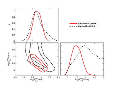
Figure 1: Constraints on the cutoff energies of the background electrons and electrons/positrons from pulsars. The bottom-left panel shows the 68% and 95% confidence regions of the two parameters, and the diagonal panels show the one-dimensional probability distributions of them. Black dashed lines and contours are for the fitting to the AMS-02 and HESS data, while red solid ones are for the AMS-02 and DAMPE data.

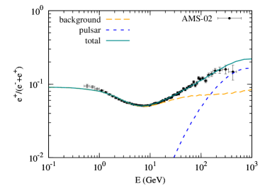
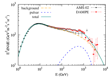
Figure 2: The positron fraction (left) and total $e^{+}+e^{-}$ fluxes (right) for the pulsar model that best-fits the AMS-02 and DAMPE data. The data points in gray are not included in the fitting.

Fig. 2 shows the best-fitting results of the positron fraction (left) and total $e^{+}+e^{-}$ fluxes (right) for the pulsar model, compared with the data. We find that the model is well consistent with the data.

III.3 DM annihilation or decay

The pair annihilation or decay of DM particles is widely postulated to be source of CR electrons/positrons Bergström (2000); Bertone et al. (2005); Bergström (2009). The DAMPE data are also expected to improve the constraints on the DM model parameters effectively. Fig. 3 shows the constraints on the mass and cross section for the annihilating DM model, assuming $\mu^{+}\mu^{-}$ annihilation channel, for fittings to AMS-02 + HESS data and AMS-02 + DAMPE data, respectively. We find that the DM parameters are much more tightly constrained in comparison with the pre-DAMPE data.

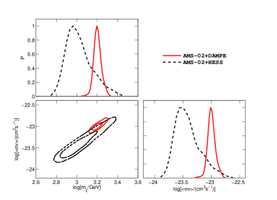
Figure 3: Same as Fig. 1 but for the constraints on the DM mass and annihilation cross section, assuming $\mu^{+}\mu^{-}$ channel.

Table 1: Best-fit $\chi^{2}$ values of the DM models through fitting to the AMS-02 + DAMPE data. The number of d.o.f. is 125.

channel	$e^{+}e^{-}$	$\mu^{+}\mu^{-}$	$\tau^{+}\tau^{-}$	$4e$	$4\mu$	$4\tau$
annihilation	214.3	139.7	135.8	147.4	130.9	133.8
decay	215.6	140.3	128.6	160.4	126.9	126.2

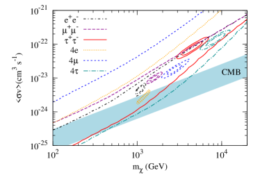
Figure 4: Favored parameter regions on the $m_{\chi}-\langle\sigma v\rangle$ (for annihilation; left) and $m_{\chi}-\tau$ (for decay; right) plane to explain the CR electron/positron data, for channels $e^{+}e^{-}$, $\mu^{+}\mu^{-}$, $\tau^{+}\tau^{-}$, $4e$, $4\mu$, and $4\tau$, respectively. The shaded region in the left panel shows the constraints from the Planck observations of CMB anisotropies, assuming an energy deposition efficiency, $f_{\rm eff}$, of $\sim 0.7$ (for $e^{+}e^{-}$ channel) to $\sim 0.15$ (for $\tau^{+}\tau^{-}$ channel) Planck Collaboration et al. (2016).

We also consider other leptonic channels of DM annihilation or decay to account for the AMS-02 and DAMPE data. Fig. 4 presents the fitting $68\%$ and $95\%$ parameter regions of $m_{\chi}$ and $\langle\sigma v\rangle$ (for annihilating DM) or $\tau$ (for decaying DM), for $e^{+}e^{-}$, $\mu^{+}\mu^{-}$, $\tau^{+}\tau^{-}$, $4e$, $4\mu$, and $4\tau$ channels. For the four-lepton cases, DM particles are assumed to first annihilate or decay into a pair of intermediate, light particles $\phi$ ($m_{\phi}<$ a few GeV), each of which decays quickly into a pair of leptons. All of these leptonic channels can give reasonably good fittings to the data. The reduced $\chi^{2}$ values of the fittings are about $1.0-1.3$ except for the $e^{+}e^{-}$ channel, for a number of degree-of-freedom (d.o.f.) of 125, as tabulated in Table 1. The annihilation or decay into $e^{+}e^{-}$ fits the data poorly, because the electron/positron spectrum is very hard that the AMS-02 positron fraction data requires a low DM mass, which is difficult to explain the DAMPE data above $\sim$TeV.

We compare the parameters derived in this work with that given in Ref. Yuan and Bi (2015) in which similar fittings to the AMS-02 and Fermi-LAT data were done. We find that the mass of DM particles required to account for the DAMPE data is larger by a factor of $\sim 2$ than that obtained through fitting to the AMS-02 and Fermi-LAT data.

The Fermi-LAT observations of dwarf spheroidal galaxies Ackermann et al. (2011); Geringer-Sameth and Koushiappas (2011); Sming Tsai et al. (2013); Ackermann et al. (2015a); Li et al. (2016) and the Planck observations of CMB anisotropies Planck Collaboration et al. (2016) give effective and robust constraints on the annihilating DM models. For the decaying DM, the extragalactic $\gamma$-ray background (EGRB) is especially suitable to constrain the DM model parameters Chen et al. (2010); Hütsi et al. (2010); Cirelli et al. (2012); Cheng et al. (2017). We use the LikeDM code Huang et al. (2017) to calculate the constraints from Fermi-LAT observations of a population of dwarf spheroidal galaxies (for annihilating DM models) and the EGRB Ackermann et al. (2015b) (for decaying DM models). In Fig. 4 we overplot the constraints on the annihilating (left) and decaying (right) DM model parameters on the $m_{\chi}-\langle\sigma v\rangle$ or $m_{\chi}-\tau$ plane. For annihilating DM models, we find that the channels with tauons will produce too many photons and exceed the upper limits set by $\gamma$-ray observations of dwarf galaxies. The channels with $e$ or $\mu$ final state particles can survive the constraints. However, when compared with the upper limits set by CMB (shaded region, with an energy deposition efficiency of $f_{\rm eff}\sim 0.15-0.7$; Slatyer et al. (2009)), none of these channels can survive. For decaying DM models, the recent EGRB data also tend to severely constrain all the models to explain the CR lepton data. Compared with recent studies Liu et al. (2017); Cheng et al. (2017) which showed that decaying DM models with $e^{+}e^{-}$ or $\mu^{+}\mu^{-}$ channels could (partially) survive the EGRB constraints, the different conclusion obtained here is primarily due to that the DAMPE data push the DM particle mass to the heavier end where the constraints are stronger. These results suggest that to account for the electron/positron excesses in the framework of DM, more tuning beyond the current simplified DM models is required.

III.4 Physical origin of the background electron spectrum

The fittings reveal that the energy spectrum of background electrons has a first break (softening) at several GeV, a second break (hardening) at $O(100)$ GeV, and a cutoff at $\sim$TeV. The GeV break may be due to the ion-neutral collisions around shocks which modifies (steepens) the accelerated particle spectrum Malkov et al. (2011). The spectral hardening and cutoff may have a common origin, i.e., the breakdown of continuous source distribution and imprint of nearby source(s) Aharonian et al. (1995); Lee et al. (2011); Di Mauro et al. (2014). As a rough estimate, the total supernova rate in a volume within 1 kpc from the Earth, which is the effective transport range of TeV electrons, is about $(1/15)^{2}\times 10^{-2}\sim 5\times 10^{-5}$ yr^-1 assuming a total rate of $10^{-2}$ yr^-1 in the Milky Way. The number of supernovae within the cooling time of $\sim 3\times 10^{5}$ yr is about 10. Observationally we indeed find roughly such a number of nearby and fresh pulsars and/or SNRs Delahaye et al. (2010). Therefore the discreteness of those sources should be important in regulating the TeV electron spectrum.

Alternatively, the break might be due to the cutoff of acceleration electron spectrum at the source. This scenario is similar to the “poly-gonato” model to explain the knee of the total CR spectra Hörandel (2003), i.e., the sum of sources with different cutoff energies gives rise to the spectral break. Observationally, however, we do find that many sources can actually accelerate electrons to energies well beyond TeV Rieger et al. (2013). Therefore, a fine tuning of the source luminosity function of different cutoff energies may be needed to explain the data.

IV Interpretations of the peak feature at $\sim 1.4$ TeV

The tentative spectral peak needs a very unusual intrinsic spectrum. It also imposes a very stringent constraint on the distance of the source, because the cooling would effectively smooth out the spectral features. For continuous injection, the cooled electron spectrum should be $\propto E^{-2}$ at high energies ($>$ a few tens of GeV where synchrotron and ICS coolings dominate), which is too soft to be consistent with the data. The characteristic cooling timescale of the electrons can be estimated as (with Eq. (1), it is straightforward to show that the first two terms are sub-dominant for the cooling of TeV electrons)

$$\tau_{\rm cool}\sim 3\times 10^{5}~{}{\rm yr}~{}\left(\frac{u_{\rm tot}}{\rm eV~{}cm^{-3}}\right)^{-1}\left(\frac{E}{\rm TeV}\right)^{-1},$$ (3)

where $u_{\rm tot}$ is the total energy density of the interstellar radiation field and the magnetic field. The travel distance of these electrons is limited to

$$\lambda\sim 0.8~{}{\rm kpc}~{}\left(\frac{D_{0}}{10^{28}~{}{\rm cm^{2}~{}s^{-1}}}\right)^{1/2}\left(\frac{u_{\rm tot}}{\rm eV~{}cm^{-3}}\right)^{-1/2}\left(\frac{E}{\rm TeV}\right)^{-1/3}.$$ (4)

Therefore the new electron source should be relatively nearby.

IV.1 Astrophysical interpretations of the DAMPE peak

IV.1.1 Energetics

We consider instantaneous injection of electrons/positrons from the source. In this case a source locating at a distance of $R_{\rm s}$ should have a lifetime $\tau>\tau_{\rm s}$, where

$$\tau_{\rm s}\sim R_{\rm s}^{2}/4D(E)\sim 8~{}{\rm kyr}~{}\left(\frac{R_{\rm s}}{0.1~{}{\rm kpc}}\right)^{2}\left(\frac{D(E)}{10^{29}~{}{\rm cm^{2}~{}s^{-1}}}\right)^{-1}.$$ (5)

The total energy of the source released can be roughly estimate as

$$\varepsilon_{\rm tot} \sim {4\pi\over 3}\left(2\sqrt{D(E)\tau_{\rm s}}\right)^{3}w_{\rm e}$$ (6)

$$\sim 10^{46}~{}{\rm erg}~{}\left(\frac{D(E)}{10^{29}~{}{\rm cm^{2}~{}s^{-1}}}\right)^{3/2}\left(\frac{\tau_{\rm s}}{10^{5}~{}{\rm yr}}\right)^{3/2}$$

$$\times \left({w_{\rm e}\over 1.2\times 10^{-18}~{}{\rm erg~{}cm^{-3}}}\right),$$

where $w_{e}$ is the energy density of the TeV peak. Clearly, for $\tau_{\rm s}\sim\tau_{\rm cool}\sim 3\times 10^{5}~{}{\rm yr}$ and $D({\rm TeV})\sim 3.3\times 10^{29}$ cm² s^-1, we have $\varepsilon_{\rm tot}\sim 3\times 10^{47}~{}{\rm erg}$, which is possible for a pulsar with a rotation period shorter than $\sim 0.1~{}{\rm s}$.

To account for the DAMPE peak, the age of the source needs to be relatively young (e.g., $\lesssim 10^{5}$ yr) and the distance needs to be close enough (e.g., $\lesssim 1$ kpc). A few sources may satisfy these conditions, such as Geminga, Monogem, Vela, Loop I, Cygnus Loop and so on Fan et al. (2010); Profumo (2012).

IV.1.2 Injection energy spectrum

While typical cutoff power-law spectrum from such astrophysical source(s) could be able to explain the observed electron/positron excesses, the peak structure in DAMPE spectrum requires quasi-monochromatic injection of particles from the sources. The cold, ultra-relativistic $e^{+}e^{-}$ plasma wind from pulsars located in the local bubble provides a possible source of such electrons and positrons Kennel and Coroniti (1984); Aharonian et al. (2012a, b). The Lorentz factor of the bulk flow of pulsar winds is suggested to be $\sim 10^{6}$, which just corresponds to the energy of the DAMPE peak. Furthermore, the density cavity of the local bubble, in which our solar system lies, makes pulsar winds less likely to form PWN, and the winds can easily escape and transport to the Earth without modification of the energy spectrum. Alternatively, Ref. Jin et al. (2016) proposed a scenario of the interaction between electrons and a kind of hypothetical particles to produce quasi-monochromatic spectrum of electrons.

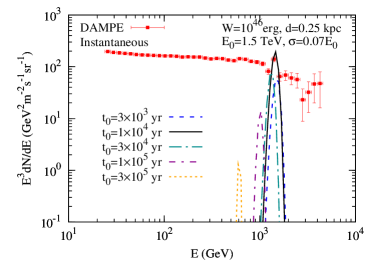
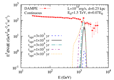
Figure 5: Fluxes of total $e^{+}+e^{-}$ from relativistic winds of a nearby pulsar. The left panel is for instantaneous injection, and the right one is for continuous injection. The injection spectrum is assumed to be Gaussian with mean energy of $E_{0}=1.5$ TeV and width of $\sigma=0.07~{}E_{0}$.

We assume a Gaussian spectrum to approximate the quasi-monochromatic injection spectrum of electrons/positrons. Fig. 5 shows the expected $e^{+}+e^{-}$ fluxes for instantaneous (left) and continuous (right) injection of such relativistic $e^{+}e^{-}$ winds from a nearby pulsar with a distance of $d=0.25$ kpc. The central energy is assumed to be $E_{0}=1.5$ TeV, and the width is $\sigma=0.07~{}E_{0}$. Different lines represent different injection time.

For instantaneous injection, two effects are clearly shown. First, we can see a remarkable cooling effect on the spectrum. The earlier the injection, the lower the cutoff energy. Second, an earlier injection also means a larger diffusion length, and hence a lower flux. We can simply estimate the diffusion length as $\lambda\sim 2\sqrt{Dt}\approx 0.2~{}{\rm kpc}~{}(E/{\rm TeV})^{1/6}(t/10^{4}\,{\rm yr})^{1/2}$. As long as $t\gtrsim 10^{4}$ yr, we have $\lambda\gtrsim 0.2$ kpc for TeV electrons, and hence $F\propto\lambda^{-3}\propto t^{-3/2}$. To match the data, the required injection energy of the pulsar is about $10^{46}-10^{48}$ erg, depending on the injection time. Such a value is, however, a little bit lower than that as expected from a typical pulsar Malyshev et al. (2009); Yin et al. (2013).

For continuous injection, we find that with the increase of the integral time, the high energy flux keeps on increasing until a certain level when an equillbrium between injection and cooling is reached. Furthermore, there are more low energy particles for longer injection time. This is because for lower energy particles more time is needed for the injected high energy ones to cool down. In the continuous injection scenario, the spectrum is typically broader than that of instantaneous injection, unless the source is fresh enough that cooling is unimportant. The luminosity of the source, $\sim 10^{34}-10^{36}$ erg s^-1, is again relatively low compared with that of a typical pulsar.

IV.1.3 “Realistic” pulsar model to account for the electron/positron data

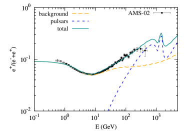
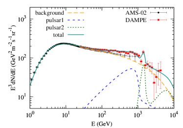
Figure 6: The positron fraction (left) and total $e^{+}+e^{-}$ fluxes (right) for the model with two nearby pulsars. The background is the same as that in Fig. 2.

For a realistic pulsar model, the spin-down luminosity decays as $t^{-2}$ after the characteristic decay time $\tau_{\rm dec}$ which is typically $10^{3}-10^{4}$ yr Malyshev et al. (2009); Profumo (2012). Furthermore, the quasi-monochromatic injection spectrum may be too ideal. In reality, a relativistic Maxwellian distribution, $f(E)\propto E^{2}\exp(-E/\Theta)$ with $\Theta$ being the electron temperature, may be more proper to describe the energy spectrum of the cold, untra-relativistic $e^{+}e^{-}$ wind. We show in Fig. 6 an illustration of the positron fraction (left) and total $e^{+}+e^{-}$ spectrum (right) from two such “realistic” pulsars. The injection luminosity is assumed to be a time-dependent form, $L=L_{0}\left(1+t/\tau_{\rm dec}\right)^{-2}$. For pulsar 1, the injection electron/positron spectrum is assumed to be a cutoff power-law form, $f(E)\propto E^{-\alpha}\exp(-E/E_{\rm max})$, which could be due to acceleration and/or cooling in the nebula. For pulsar 2, we assume a Maxwellian distribution of the injection wind particles. The model parameters are tabulated in Table 2. We can see in Fig. 6 that there are high energy tails of the pulsar components, which are due to late time injection (see e.g., Aharonian et al. (1995)). The main peaks come from the early time injection ($t<\tau_{\rm dec}$).

Table 2: Parameters of the two pulsars as shown in Fig. 6.

	$d$	$L_{0}$	$t_{\rm age}$	$\tau_{\rm dec}$	$\alpha$	$E_{\rm max}$ ($\Theta$)
	(kpc)	(erg s-1)	(kyr)	(kyr)		(TeV)
pulsar 1	0.25	$5.3\times 10^{37}$	260	3.0	1.7	3.0
pulsar 2	0.25	$0.9\times 10^{37}$	180	3.0	$-2.0$	2.0

Pulsar 1 is employed to account for the positron and electron excesses below TeV. It may be Geminga- or Monogem-like (e.g., Hooper et al. (2009a); Yüksel et al. (2009); Linden and Profumo (2013); Yin et al. (2013)). The initial spin-down luminosity is estimated to be about $5\times 10^{37}$ erg s^-1, which is smaller by a factor of $\sim 10$ than that of the crab pulsar. This value is not unusual, since the crab pulsar is among the fastest rotating family of normal pulsars Faucher-Giguère and Kaspi (2006). It is also possible that the ensemble of a large population of pulsars in the Milky Way plays the role of pulsar 1 Malyshev et al. (2009); Yin et al. (2013). In such a case, wiggles may be seen in the spectrum Malyshev et al. (2009) (see, however, Kawanaka et al. (2010)).

Pulsar 2 is introduced to explain the DAMPE peak. Its properties are more unique. First, the $e^{+}e^{-}$ winds should be directly injected into the interstellar space without effective acceleration by the SNR/PWN. This implies that either the pulsar moves fast away from the SNR, or the supernova explodes in a density cavity (e.g., the local bubble) and the ejecta expands fast without significant deceleration. Second, moderate cooling of electrons is necessary to form a peak of the spectrum, otherwise the spectrum would be too broad for Maxwellian injection. This requires that the pulsar should be middle-aged (mature). On the other hand, the pulsar’s age should not be too large to make most of the electrons cool down to energies lower than TeV. Therefore the age of pulsar 2 is constrained to be about $10^{5}$ yr. The initial spin-down luminosity of pulsar 2 is about $10^{37}$ erg s^-1, two orders of magnitude lower than the current crab pulsar’s spin-down luminosity. This luminosity is also reasonable, suggesting a rotation period of $\sim 0.15~{}{\rm s}~{}(L/10^{37}~{}{\rm erg~{}s^{-1}})^{1/4}~{}(B/10^{13}~{}{\rm G})^{-1/2}$ for a neutron star radius $\sim 10$ km. In Ref. Vranesevic et al. (2004) it was shown that $\sim 40\%$ normal pulsars are born with periods of $0.1-0.5$ s, about an order of magnitude longer than that of the crab pulsar.

For the pulsars assumed in the above discussion, the surface magnetic field can be estimated as $B=8.6\times 10^{12}(P/0.1~{}{\rm s})~{}(\tau_{\rm dec}/10^{4}~{}{\rm yr})^{-1/2}$ G $\sim 10^{13}$ G Kawanaka et al. (2010). Therefore mildly magnetized pulsar is needed to explain the data.

We conclude that a middle-aged, relatively slowly-rotated, mildly magnetized, isolate pulsar in the local bubble is a possible candidate source of the DAMPE peak. There may be more than one pulsars like pulsar 2 in the local environment. In that case we may expect to see more such peaks in the electron spectrum. The future measurement of the electron spectrum to higher energies by DAMPE with high energy resolution will critically test this scenario.

IV.2 DM annihilation interpretations of the DAMPE peak

IV.2.1 General consideration

Suppose the source injects monoenergetic electrons at a continuous rate $\dot{Q}$, the radial energy density distribution of electrons can be approximately as HESS Collaboration et al. (2016)

$$w_{\rm e}(R)={\dot{Q}\over 4\pi D(E)R}{\rm erfc}(R/\lambda).$$ (7)

Note that for monoenergetic electrons the above equation holds only for $R\ll\lambda$; otherwise the cooling effect can not be ignored any more. Under such a condition we have $w_{\rm e}(R)\approx\dot{Q}/[4\pi D(E)R]$, and the source injection power is

$$\dot{Q} \approx 5\times 10^{32}~{}{\rm erg~{}s^{-1}}~{}\left({R\over 0.1~{}{\rm kpc}}\right)\left({D(E)\over 10^{29}~{}{\rm cm^{2}~{}s^{-1}}}\right)$$ (8)

$$\times \left({w_{\rm e}\over 1.2\times 10^{-18}~{}{\rm erg~{}cm^{-3}}}\right).$$

In the case of a DM sub-halo with a dense core whose size is $\delta$, the energy density of the DM particles should be (assuming $m_{\chi}\approx 1.5$ TeV)

$$\rho_{\chi} \sim 0.4~{}{\rm TeV~{}cm^{-3}}~{}\left({\dot{Q}\over 5\times 10^{32}~{}{\rm erg~{}s^{-1}}}\right)^{1/2}$$ (9)

$$\times \left[{\langle\sigma v\rangle_{\chi\chi\rightarrow e^{+}e^{-}}\over 3\times 10^{-26}~{}{\rm cm^{3}~{}s^{-1}}}\right]^{-1/2}\left({\delta\over 10~{}{\rm pc}}\right)^{-3/2},$$

where $\langle\sigma v\rangle_{\chi\chi\rightarrow e^{+}e^{-}}$ is the velocity-averaged annihilation cross section. This density is about 1000 times higher than that of the widely-taken local DM energy density. Interestingly there is another possibility that the Sun is actually in a DM-density-enhanced region. Suppose such a region has a size of $\sim 100$ pc, we have $\rho_{\chi}\sim 0.012~{}{\rm TeV~{}cm^{-3}}$, about 30 times higher than the canonical local DM energy density. Such a density enhancement seems to be not in tension with other observations Hektor et al. (2014). The total mass of the DM sub-halo or density-enhanced region reads

$$M_{\chi} \sim 4\times 10^{4}~{}M_{\odot}~{}\left({\dot{Q}\over 5\times 10^{32}~{}{\rm erg~{}s^{-1}}}\right)^{1/2}$$ (10)

$$\times \left[{\langle\sigma v\rangle_{\chi\chi\rightarrow e^{+}e^{-}}\over 3\times 10^{-26}~{}{\rm cm^{3}~{}s^{-1}}}\right]^{-1/2}~{}\left({\delta\over 10~{}{\rm pc}}\right)^{3/2}.$$

The energy spectrum of electrons at production depends on the mass of the DM particle and the annihilation final state. For the quark final state, the electrons are produced through the hadronization of quarks, which results in a very soft spectrum. The spectrum is significantly harder for the leptonic and gauge bosonic final states due to the non-zero decaying branching ratios to direct production of electrons. The hardest spectrum comes from the direct annihilation into a pair of $e^{+}e^{-}$, which gives nearly monochromatic electrons (and positrons). The peak structure of the DAMPE data requires a branching ratio to $e^{+}e^{-}$ final state, and a local origin of the DM annihilation. These requirements suggest the scenario of a nearby DM clump Hooper et al. (2009b); Brun et al. (2009) or a local DM density enhancement Hektor et al. (2014).

In order to compare with the data, we also need to include the “background” electrons/positrons. The continuous $e^{+}+e^{-}$ fluxes that derived through fitting to the wide-band data in Sec. III are assumed to be the “background” here (similar approach has been used to search for potential prominent spectral features; Bergström et al. (2013); Hooper and Xue (2013); Ibarra et al. (2014)). Specifically, the fluxes shown in Fig. 2 are adopted.

IV.2.2 Nearby DM clump

The structures of matter in the universe are hierarchical. The N-body simulations of the cold DM (CDM) structure formation reveals a large amount of subhaloes in the Galactic DM halo Gao et al. (2004); Springel et al. (2008), with the smallest subhalo mass as light as the Earth Diemand et al. (2005). The DM subhaloes were exployed to account for the “boost factor” required to explain the HEAT positron excess Yuan and Bi (2007). More detailed calculation based on the N-body simulation results showed that the “boost factor” from DM clumpiness was usually negligible Lavalle et al. (2008). Alternatively, the local DM subhalo(es) were able to play the role of an effective “boost factor” if they are close enough to the Earth Cumberbatch and Silk (2007); Hooper et al. (2009b). In addition, this scenario can give harder positron spectrum than that of the average of the whole Galaxy, which can fit the data with more conventional annihilation channels of DM (e.g., gauge bosons and quarks). However, the comparison of the required conditions with the numerical simulations shows that the probability to have such a DM clump close and massive enough is very low Lavalle et al. (2007); Brun et al. (2009). Here we revisit this nearby DM clump model in light of the DAMPE data, and investigate what condition is needed to account for the data.

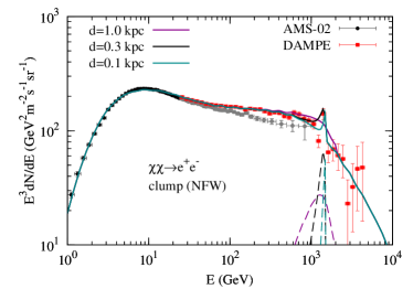
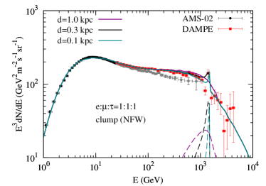
Figure 7: Fluxes of the total $e^{+}+e^{-}$, from the sum of the continuous background and the DM annihilation from a nearby clump. The left panel is for DM annihilation into a pair of $e^{+}e^{-}$, and the right one is for DM annihilation into all flavor leptons with universal couplings. Three distances of the clump, as labelled in the plot, are considered. See Table 3 for the mass of the DM particle, and the mass and annihilation luminosity of the clump.

Table 3: Mass of the DM particle, and mass and luminosity of the DM clump halo to fit the DAMPE data. The annihilation cross section is assumed to be $3\times 10^{-26}$ cm³s^-1.

channel	1.0 kpc				0.3 kpc				0.1 kpc
	$m_{\chi}$/TeV	$M_{\rm sub}$/M⊙	${\mathcal{L}}$/GeV2cm-3		$m_{\chi}$/TeV	$M_{\rm sub}$/M⊙	${\mathcal{L}}$/GeV2cm-3		$m_{\chi}$/TeV	$M_{\rm sub}$/M⊙	${\mathcal{L}}$/GeV2cm-3
$e^{+}e^{-}$	2.2	$3.8\times 10^{9}$	$1.0\times 10^{67}$		1.5	$8.0\times 10^{7}$	$3.8\times 10^{65}$		1.5	$5.0\times 10^{6}$	$3.5\times 10^{64}$
$e\mu\tau$	2.2	$1.0\times 10^{10}$	$2.3\times 10^{67}$		1.5	$2.6\times 10^{8}$	$1.0\times 10^{66}$		1.5	$1.9\times 10^{7}$	$1.1\times 10^{65}$

We assume that the density profile of the DM clump is NFW. For a clump close to the solar location, the strong tidal force of the Milky Way will remove the outer material of the clump, leaving a more compact core. We present the detailed determination of the mass distribution of a DM clump when considering the tidal stripping in the Appendix. We further assume that the annihilation cross section is $3\times 10^{-26}$ cm³s^-1, which corresponds to the value inferred from the thermal production of the DM. Fig. 7 shows the resulting $e^{+}+e^{-}$ fluxes for a DM clump locating at 1.0, 0.3, and 0.1 kpc away from the Earth. The left panel is for the $e^{+}e^{-}$ final state, and the right one is for annihilation to all flavors of charged leptons with equal branching ratios. The required DM particle mass, the total mass of the clump, and its annihilation luminosity, ${\mathcal{L}}=\int\rho^{2}dV$, are given in Table 3.

We find that a DM clump as massive as $10^{7}-10^{8}$ M_⊙ with a distance of $\sim 0.1-0.3$ kpc can account for the DAMPE data if the annihilation branching ratio to $e^{+}e^{-}$ is large enough. We have tested that for channels other than $e^{+}e^{-}$, such as $\mu^{+}\mu^{-}$, $\tau^{+}\tau^{-}$, and $W^{+}W^{-}$, no prominent peak feature can be generated. The distance of the DM clump should not be larger than a few hundred parsec so that the $\delta$-function like spectrum of electrons/positrons will not be smoothed out by the cooling. These two requirements are just consistent with what we expected in Sec. IV. A. Note also that for a distance of $1.0$ kpc, the required clump mass is about $10^{10}$ M_⊙, which is close to the maximum mass of subhalos in A Milky Way size halo Springel et al. (2008). Such a case is thus disfavored.

We need further to check that the contribution from such a DM clump dominates the Milky Way halo and other substructures so that the peak structure would not be smoothed out. Since the average enhancement due to substructures for charged particles is found to be small Lavalle et al. (2008), we consider only the Milky Way halo. It turns out that, for the $e^{+}e^{-}$ channel, $\langle\sigma v\rangle=3\times 10^{-26}$ cm³s^-1 and $m_{\chi}=1.5$ TeV, the contribution from the DM annihilation in the whole Milky Way halo is about two orders of magnitude lower than that shown in Fig. 7 at $\sim$TeV, which is thus negligible (this can also be seen from Fig. 4).

IV.2.3 Enhanced local DM density

Besides the gravitationally bound substructures, density fluctuations occur and disappear continuously in the Milky Way halo, as illustrated by numerical simulations Kamionkowski et al. (2010). An over-density region with $\rho/\rho_{0}<200\,({\rm kpc}/\delta)^{2}$, where $\rho_{0}$ is the average local density and $\delta$ is the region size, is gravitationally unbound Hektor et al. (2014). The density profile within the over-density regions may be shallower than the gravitationally bound substructures. It was proposed that a local DM density enhancement by a factor of $\sim 30-50$ within $R\sim 0.5$ kpc of the Earth and annihilation channels into gauge bosons or quarks could explain the observed positron excesses Hektor et al. (2014).

The results of the enhanced local density scenario are very similar to that of Fig. 7. To give the DAMPE peak, we need a considerable branching ratio to monochromatic $e^{+}e^{-}$ in the final states and a not too large size ($s\lesssim 0.3$ kpc) of the over-density region. If the annihilation cross section is assumed to be $\langle\sigma v\rangle=3\times 10^{26}$ cm³s^-1, the required density is about $17-35$ times of the canonical local density of $\rho_{0}=0.4$ GeV cm^-3 for the $e^{+}e^{-}$ channel.

IV.2.4 DM (sub-)structures from numerical simulations

In the above two subsections, we have shown that either a nearby DM clump or an enhanced local density is able to account for the DAMPE electron spectrum. Here we check from the numerical simulations of the DM structure formation to see whether the required conditions can be satisfied.

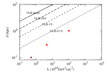
Figure 8: Required annihilation luminosity ${\mathcal{L}}$ and distance $d$ (red squares) from the Earth of the clump to fit the DAMPE data, assuming $e^{+}e^{-}$ channel, compared with the probability distributions (black lines) of finding a subhalo with ${\mathcal{L}}$ within $d$ inferred from the VLII simulations Brun et al. (2009).

Fig. 8 shows the probability distributions of finding a clump with annihilation luminosity ${\mathcal{L}}$ within distance $d$ from the Earth inferred from the Via Lactea II (VLII) simulations Diemand et al. (2008), as given in Ref. Brun et al. (2009). Red squares are the required values to account for the DAMPE electron data, as discussed in Sec. IV. B. Here the annihilation channel is assumed to be $e^{+}e^{-}$, and the cross section is fixed to be $3\times 10^{-26}$ cm³s^-1. It is shown that the probability of having a right clump to explain the data is relatively low, $p<10^{-3}$. For the annihilation to $e\mu\tau$ leptons with universal couplings, the required luminosity ${\mathcal{L}}$ is larger by a factor of 3, hence the situation is even worse. If there is moderate enhancement of the annihilation cross section from the particle physics, such as the non-thermal production of the DM Jeannerot et al. (1999); Lin et al. (2001); Yuan et al. (2012), the Sommerfeld enhancement mechanism (e.g., Sommerfeld (1931); Hisano et al. (2005); Arkani-Hamed et al. (2009)) or Breit-Wigner type resonance of the annihilation interaction Griest and Seckel (1991); Gondolo and Gelmini (1991), the required luminosity can be lower and the probability becomes higher. Alternatively, if there is mini-spike in the center of the DM clump, the annihilation luminosity may be significantly enhanced and the required mass of the clump may be much smaller Zhao and Silk (2005).

As for the enhanced local density scenario, we consider the distribution of density fluctuations. The density fluctuation was found to follow roughly a log-normal distribution with a Gaussian width of $\ln\rho$ of $\sim 0.2$ Kamionkowski et al. (2010). Therefore an over-density of $20$ times of the local average density indicates a $\sim 15\sigma$ deviation from the mean value. This probability, again, is very low. Note, however, the distribution of density fluctuation has a power-law tail at large $\rho$, due to substructures Kamionkowski et al. (2010). Therefore the actual probability to have an over-density region should be higher than the above estimate. Furthermore, if there is enhancement of the annihilation cross section the required over-density factor can be smaller.

IV.2.5 Gamma-ray constraints

The annihilation of DM will produce $\gamma$-ray photons accompanied with electrons/positrons, from the internal bremsstrahlung process for the charged fermion channel and/or the decay of the final state particles. We check whether such $\gamma$-ray emission can be detectble or constrained by the current observations.

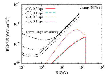
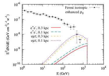
Figure 9: Left: expected $\gamma$-ray fluxes from the annihilation of DM in a nearby clump. The integral radius is chosen to be $1^{\circ}$. The dot-dashed lines show the 10-year point source sensitivities of Fermi-LAT with the Pass 8 instrument response for directions of $(l,b)=(0,0)$, $(0,30^{\circ})$, $(0,90^{\circ})$, and $(120^{\circ},45^{\circ})$ from top to bottom. Right: expected $\gamma$-ray fluxes from the annihilation of DM in the enhanced local density model, compared with the isotropic background measurements by Fermi-LAT Ackermann et al. (2015b).

We calculate the expected $\gamma$-ray fluxes from the DM annihilation for the models which can potentially explain the DAMPE electron data, i.e., with $e^{+}e^{-}$ or $e\mu\tau$ channels and a distance (for the clump) or radius (for the enhanced local density scenario) of $\leq 0.3$ kpc. For the nearby clump scenario, the $\gamma$-ray emission is essentially extended. For simplicity, we integrate the emission within $1^{\circ}$ radius, and compare them with the 10-year point source sensitivity of Fermi-LAT with the Pass 8 instrument response. For the enhanced local density scenario, the $\gamma$-ray emission is diffuse. Therefore we employ the Fermi-LAT isotropic background data as constraints Ackermann et al. (2015b). The results are shown in Fig. 9. We find that except for the annihilation to $e\mu\tau$ case of the enhanced DM density model which exceeds the highest point of the Fermi-LAT isotropic background marginally, other cases are not in conflict with Fermi-LAT observations.

IV.2.6 Particle model of DM

In this sub-section we discuss possible DM particle models which are able to interpret the DAMPE peak, and the relevant constraints from the relic density.

Lepton Portal DM model — Following Bai and Berger (2014), we discuss the lepton portal DM models. If DM particles are fermions, the interaction between DM and leptons can be written as

$$\mathcal{L}_{\rm fermion}\supset\lambda_{i}\phi_{i}\bar{\chi}_{L}e_{R}^{i}+h.c.,$$ (11)

where $\chi$ denotes the DM particle, $e^{i}=e,\mu,\tau$ represents charged leptons, and $\phi_{i}$ is the charged scalar mediator with unit lepton number. In this model, we have only two parameters (the coupling strength $\lambda_{i}$ and the mass of the mediator $m_{\phi,i}$) for each flavor. To avoid the decay of DM, $m_{\chi}$ should be smaller than the mass of the mediator.

If DM particles are Dirac fermions, the annihilation cross section is

$$\frac{1}{2}\,(\sigma v)^{\chi\bar{\chi}}_{\rm{Dirac}} = \frac{1}{2}\left[\frac{\lambda^{4}m_{\chi}^{2}}{32\,\pi\,(m_{\chi}^{2}+m_{\phi}^{2})^{2}}\right.$$

$$+ \left.v^{2}\frac{\lambda^{4}\,m_{\chi}^{2}\,(-\,5m_{\chi}^{4}\,-\,18m_{\chi}^{2}m_{\phi}^{2}+11m_{\phi}^{4})}{768\,\pi\,(m_{\chi}^{2}+m_{\phi}^{2})^{4}}\right],$$

where $v$ is the relative velocity between two DM particles and the factor $1/2$ accounts for the difference between particle and anti-particle of Dirac DM. Here we neglect the mass of leptons, and assume that $\lambda_{e}=\lambda_{\mu}=\lambda_{\tau}\equiv\lambda$. Obviously, the cross section is not velocity suppressed in this model.

We calculated the relic density of DM using micrOMEGAs Bélanger et al. (2007). The parameters that produce the correct DM relic density, $\Omega_{DM}h^{2}=0.119$, for different values of $m_{\phi}$ are shown in the left panel of Fig. 10. The corresponding annihilation cross section ($\langle\sigma v\rangle/2$) is shown in the right panel of Fig. 10 and the factor of 1/2 accounts for the fact that Dirac DM consists of both a particle and an anti-particle. In the previous sub-section, we set $\langle\sigma v\rangle=3\times 10^{-26}$ cm³s^-1 and get the corresponding annihilation luminosity $L=\int\rho^{2}dV$. From Fig. 10, we can see that there is a slight deviation of the DM annihilation cross section from the canonical value $3\times 10^{-26}$ cm³s^-1. So the annihilation luminosity should be

$$L=L^{\prime}\times\frac{3\times 10^{-26}{\rm cm^{3}s^{-1}}}{1/2\langle\sigma v\rangle}.$$

Here $L^{\prime}$ is the annihilation luminosity presented in Table 3.

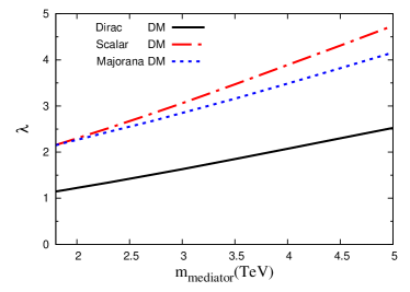
Figure 10: The coupling constants $\lambda$ as functions of the mediator mass that give the correct relic density (left), and the corresponding annihilation cross section for the Dirac fermion model (right).

For the Majorana DM case, the annihilation cross section is

$$(\sigma v)^{\chi\chi}_{\rm{Majorana}}=v^{2}\,\frac{\lambda^{4}\,m_{\chi}^{2}\,(m_{\chi}^{4}+m_{\phi}^{4})}{48\pi\,(m_{\chi}^{2}+m_{\phi}^{2})^{4}}\,.$$ (13)

Setting $\rm{m_{\chi}=1.5~{}TeV}$, we get the parameters that give the correct relic density, which are also shown in Fig. 10. The DM annihilation cross section is p-wave suppressed by the small velocity of DM particles. The typical velocity of DM particles is about $0.3c$ at freeze-out and $\sim 10^{-3}c$ at present. Therefore a boost factor of $10^{4}\sim 10^{5}$ is necessary. The Sommerfeld enhancement is a natural mechanism that could enhance the DM annihilation cross section for low relative velocities DM particles Sommerfeld (1931); Hisano et al. (2005); Arkani-Hamed et al. (2009). Other mechanisms such as the Breit-Wigner resonance was also proposed Griest and Seckel (1991); Gondolo and Gelmini (1991).

Then we consider the complex scalar DM model whose interaction can be written as

$${\cal L}_{\rm scalar}\supset\lambda_{i}X\overline{\psi^{i}}_{L}e_{R}^{i}\,+\,h.c.,$$ (14)

where $X$ denotes the DM particle and the mediator $\psi$ is a Dirac fermion with electric charge $-1$ and the corresponding lepton number. Here we only consider the complex scalar DM model because the direct detection rate can be effectively suppressed in this case Barger et al. (2008). The cross section is

$$\frac{1}{2}\,(\sigma v)^{\chi\chi^{\dagger}}_{\rm complex\,scalar}\,=\,\frac{1}{2}\,\left[v^{2}\,\frac{\lambda^{4}\,m_{X}^{2}}{48\,\pi\,(m_{X}^{2}+m_{\psi}^{2})^{2}}\right]\,.$$ (15)

The annihilation cross section is also p-wave suppressed. The coupling and cross section correspond to the observed DM relic density are shown in Fig. 10.

Lepton Flavored DM model — In the lepton portal DM model, DM particles annihilate into leptons through lepton-flavored mediators. We can also assume that the DM particles have electron lepton number for Dirac and complex scalar DM model. In such a model, the DM particles could only annihilate into electrons and positrons. The Lagrangian is the same as the previous lepton portal DM models. To get the same annihilation cross section and hence the correct relic density with the previous model, the coupling parameter needs to be $\sqrt[4]{3}=1.3$ times larger according to Eqs. (IV.2.6) and (15).

TeV Right-handed Neutrino DM model — One of the TeV right-handed neutrino models can be described by the following Lagrangian Krauss et al. (2003); Cheung and Seto (2004)

$${\cal L}_{\rm int} = f_{\alpha\beta}L^{T}_{\alpha}Ci\tau_{2}L_{\beta}S^{+}_{1}+g_{1\alpha}N_{1}S_{2}^{+}\ell_{\alpha R}+g_{2\alpha}N_{2}S_{2}^{+}\ell_{\alpha R}+h.c.$$ (16)

$$+ \,M_{N_{1}}N^{T}_{1}CN_{1}+M_{N_{2}}N^{T}_{2}CN_{2}-V(S_{1},S_{2}),$$

where $N_{1,2}$ are right-handed neutrinos, $L_{\alpha,\beta}$ and $l_{\alpha R}$ are the lepton doublet and singlet, $\alpha,\beta$ are the family indices, $C$ is the charge-conjugation operator, $V(S_{1},S_{2})$ is the scalar potential which contains two complex scalar fields ($S_{1}$, $S_{2}$), and $f_{\alpha\beta}$ is the anti-symmetric coupling matrix. The lighter one of the two right-handed neutrinos (denoted as $N$ here) can be the DM candidate. In this model, the DM particles annihilate into $e^{+}e^{-}$, $\mu^{+}\mu^{-}$ and $\tau^{+}\tau^{-}$ through $t$- and $u$-channel with an intermediate $S_{2}^{+}$. The cross section is given by

$$(\sigma v)_{\alpha} = \frac{g_{1\alpha}^{4}}{64\pi}\,\frac{1}{s}\;\int_{-1}^{1}\;dx\;\Biggr{\{}\frac{s^{2}(1-\beta_{N}x)^{2}}{4\left[M_{N}^{2}-M_{S_{2}}^{2}-\frac{s}{2}(1-\beta_{N}x)\right]^{2}}$$

$$+ \frac{s^{2}(1+\beta_{N}x)^{2}}{4\left[M_{N}^{2}-M_{S_{2}}^{2}-\frac{s}{2}(1+\beta_{N}x)\right]^{2}}$$

$$- \frac{2M_{N}^{2}s}{\left[M_{N}^{2}-M_{S_{2}}^{2}-\frac{s}{2}(1-\beta_{N}x)\right]\left[M_{N}^{2}-M_{S_{2}}^{2}-\frac{s}{2}(1+\beta_{N}x)\right]}\Biggr{\}}.$$

From the above equation we can see that $\sigma v\to 0$ for $v\to 0$, since $\beta_{N}=\left(1-4M^{2}_{N}/s\right)^{1/2}\sim 0$. The cross section is also $p$-wave suppressed, which is common for identical Majorana fermions Goldberg (1983).

V Anisotropies

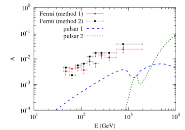
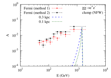
Figure 11: Dipole anisotropy of $e^{+}+e^{-}$ fluxes from the two-pulsar model (left) as shown in Fig. 6 and the DM subhalo model (right) as shown in Fig. 7. The 95% upper limits from Fermi-LAT observations are also shown Abdollahi et al. (2017b).

The anisotropies of high energy electrons can effectively test the local origin models. The amplitude of the dipole anisotropy can be calculated as

$$A=\frac{3D(E)}{c}\frac{|\nabla\phi_{e}|}{\phi_{e}},$$ (18)

where $\phi_{e}$ is the local flux of $e^{+}+e^{-}$. Assuming the background is isotropic, we calculate the anisotropies of the pulsar model (see Fig. 6) and DM subhalo model (see Fig. 7). The results are shown in Fig. 11.

For the pulsar model, the anisotropies from both sources are about $10^{-3}-10^{-2}$ at TeV energies. The high energy tails from pulsars give relatively high anisotropies, although their fluxes are small. This is because fresh particles injected just recently have smaller diffusion distance, and hence give larger gradient than earlier injected ones. We should keep in mind that the anisotropy of pulsar 1 is largely uncertain, depending on the model parameters (mainly the age) assumed Grasso et al. (2009). The age of pulsar 2 is better constrained, and its anisotropy prediction is more robust. If the injection spectrum of pulsar 2 is narrower than the Maxwellian distribution, then the age of pulsar 2 can be smaller, and hence a larger anisotropy is possible. For the DM subhalo model, the anisotropies can be as large as a few percents around the DAMPE peak.

Compared with the upper limits obtained with seven years of Fermi-LAT observations Abdollahi et al. (2017b), the expected anisotropies for both models are consistent with the data. Future experiments such as the High Energy cosmic-Radiation Detection facility (HERD; Zhang et al. (2014)) and the Cherenkov Telescope Array (CTA; Actis et al. (2011)) may reach a sensitivity of $\sim 10^{-3}$ around TeV energies and can effectively test these models Fang et al. (2017b); Linden and Profumo (2013).

VI Conclusion

The precise measurements about the high energy electron (including positron) spectrum by DAMPE are very helpful in understanding the origin of CR electrons. In this work we extensively discuss the physical implications of the DAMPE data. Both the astrophysical models and the exotic DM annihilation/decay scenarios are examined. Our findings are summarized as follows.

• The spectral softening at $\sim 0.9$ TeV suggests a cutoff (or break) of the background electron spectrum, which is expected to be due to either the discretness of CR source distributions in both space and time, or the maximum energies of electron acceleration at the sources. The DAMPE data enables a much improved determination of the cutoff energy of the background electron spectrum, which is about $3$ TeV assuming an exponential form, compared with the pre-DAMPE data.

• Both the annihilation and decay scenarios of the simplified DM models to account for the sub-TeV electron/positron excesses are severely constrained by the CMB and/or $\gamma$-ray observations. Additional tuning of such models, through e.g., velocity-dependent annihilation, is required to reconcile with those constraints.

• The tentative peak at $\sim 1.4$ TeV suggested by DAMPE implies that the sources should be close enough to the Earth ($\lesssim 0.3$ kpc) and inject nearly monochromatic electrons into the Galaxy. We find that the cold and ultra-relativistic $e^{+}e^{-}$ wind from pulsars is a possible source of such a structure. Our analysis further shows that the pulsar should be middle-aged, relatively slowly-rotated, mildly magnetized, and isolate in a density cavity (e.g., the local bubble).

• An alternative explanation of the peak is the DM annihilation in a nearby clump or a local density enhanced region. The distance of the clump or size of the over-density region needs to be $\lesssim 0.3$ kpc. The required parameters of the DM clump or over-density are relatively extreme compared with that of numerical simulations, if the annihilation cross section is assumed to be $3\times 10^{-26}$ cm³ s^-1. Specifically, a DM clump as massive as $10^{7}-10^{8}$ M_⊙ or a local density enhancement of $17-35$ times of the canonical local density is required to fit the data if the annihilation product is a pair of $e^{+}e^{-}$. Moderate enhancement of the annihilation cross section would be helpful to relax the tension between the model requirement and the N-body simulations of the CDM structure formation. The DM clump model or local density enhancement model is found to be consistent with the Fermi-LAT $\gamma$-ray observations.

• The expected anisotropies from either the pulsar model or the DM clump model are consistent with the recent measurements by Fermi-LAT. Future observations by e.g., CTA, will be able to detect such anisotropies and test different models.

DAMPE will keep on operating for a few more years. More precise measurements of the total $e^{+}+e^{-}$ spectrum extending to higher energies are available in the near future. Whether there are more structures in the high energy window, which can critically distinguish the pulsar model from the DM one, is particularly interesting. With more and more precise measurements, we expect to significantly improve our understandings of the origin of CR electrons.

Appendix A Density profiles of DM subhalos in the solar neighborhood

We follow the results of high-resolution N-body simulation Aquarius to determine the density profile of a DM subhalo in the solar neighborhood Springel et al. (2008). The NFW profile was found to give reasonable fit to the density profile of subhalos. The concentration of a subhalo, defined as the mean overdensity within the radius at which the maximum circular velocity is attained ($r_{\rm max}$) in units of the critical density, is found to vary with both the subhalo mass and the spatial location. For the solar neighborhood, we find approximately

$$\delta_{V}=1.2\times 10^{6}\left(M_{\rm sub}/10^{6}\,M_{\odot}\right)^{-0.18},$$ (19)

where $M_{\rm sub}$ is the mass of a subhalo (after the tidal stripping). The concentional NFW concentration parameter, $c\equiv r_{v}/r_{s}$ where $r_{v}$ is the virial radius and $r_{s}$ is the scale radius, relates with $\delta_{V}$ through

$$7.213~{}\delta_{V}=\delta_{c}=\frac{200}{3}\frac{c^{3}}{\ln(1+c)-c/(1+c)}.$$ (20)

The tidal force from the main halo will remove the outer matter of a subhalo, especially when it is close to the Milky Way center. This tidal radius can be approximated as the radius at which the density is 0.02 times of the local average unbound density (i.e., $0.4$ GeV cm^-3 at the solar neighborhood). We find that the tidal radius is roughly $0.2$ times of the original virial radius of a subhalo, and the enclose mass is about half of the original mass of $M_{\rm sub}^{\prime}$. So our procedure to determine the density profile of a subhalo with tidal stripping is as follows:

• Given a subhalo mass $M_{\rm sub}$, calculate its concentration with Eq. (19).

• Calculate the “original” density profile of the subhalo with $M_{\rm sub}^{\prime}=2M_{\rm sub}$ and the concentration.

• Calculate the tidal radius $r_{t}$ of the subhalo, and remove the DM outside of $r_{t}$.

References

- Shen (1970) C. S. Shen, Astrophys. J. Lett. 162, L181 (1970).
- Harding and Ramaty (1987) A. K. Harding and R. Ramaty, International Cosmic Ray Conference 2, 92 (1987).
- Aharonian et al. (1995) F. A. Aharonian, A. M. Atoyan, and H. J. Voelk, Astron. Astrophys. 294, L41 (1995).
- Chi et al. (1996) X. Chi, K. S. Cheng, and E. C. M. Young, Astrophys. J. Lett. 459, L83 (1996).
- Zhang and Cheng (2001) L. Zhang and K. S. Cheng, Astron. Astrophys. 368, 1063 (2001).
- Bergström (2000) L. Bergström, Reports of Progress in Physics 63, 793 (2000), eprint hep-ph/0002126.
- Bertone et al. (2005) G. Bertone, D. Hooper, and J. Silk, Phys. Rept. 405, 279 (2005), eprint hep-ph/0404175.
- Bergström (2009) L. Bergström, New Journal of Physics 11, 105006 (2009), eprint 0903.4849.
- Adriani et al. (2009) O. Adriani, et al., Nature 458, 607 (2009), eprint 0810.4995.
- Ackermann et al. (2012a) M. Ackermann, et al., Phys. Rev. Lett. 108, 011103 (2012a), eprint 1109.0521.
- Aguilar et al. (2013) M. Aguilar, et al., Phys. Rev. Lett. 110, 141102 (2013).
- Accardo et al. (2014) L. Accardo, et al., Phys. Rev. Lett. 113, 121101 (2014).
- Chang et al. (2008) J. Chang, et al., Nature 456, 362 (2008).
- Aharonian et al. (2008) F. Aharonian, et al., Phys. Rev. Lett. 101, 261104 (2008), eprint 0811.3894.
- Abdo et al. (2009) A. A. Abdo, et al., Phys. Rev. Lett. 102, 181101 (2009), eprint 0905.0025.
- Aguilar et al. (2014a) M. Aguilar, et al., Phys. Rev. Lett. 113, 121102 (2014a).
- Aguilar et al. (2014b) M. Aguilar, et al., Phys. Rev. Lett. 113, 221102 (2014b).
- Fan et al. (2010) Y.-Z. Fan, B. Zhang, and J. Chang, International Journal of Modern Physics D 19, 2011 (2010), eprint 1008.4646.
- Serpico (2012) P. D. Serpico, Astroparticle Physics 39, 2 (2012), eprint 1108.4827.
- Bergström et al. (2008) L. Bergström, T. Bringmann, and J. Edsjö, Phys. Rev. D 78, 103520 (2008), eprint 0808.3725.
- Ibarra et al. (2009) A. Ibarra, A. Ringwald, D. Tran, and C. Weniger, J. Cosmol. Astropart. Phys. 8, 017 (2009), eprint 0903.3625.
- Cirelli (2012) M. Cirelli, Pramana 79, 1021 (2012), eprint 1202.1454.
- Bi et al. (2013) X.-J. Bi, P.-F. Yin, and Q. Yuan, Frontiers of Physics 8, 794 (2013), eprint 1409.4590.
- Gaskins (2016) J. M. Gaskins, Contemporary Physics 57, 496 (2016), eprint 1604.00014.
- Hooper et al. (2009a) D. Hooper, P. Blasi, and P. Dario Serpico, J. Cosmol. Astropart. Phys. 1, 25 (2009a), eprint 0810.1527.
- Yüksel et al. (2009) H. Yüksel, M. D. Kistler, and T. Stanev, Phys. Rev. Lett. 103, 051101 (2009), eprint 0810.2784.
- Profumo (2012) S. Profumo, Central European Journal of Physics 10, 1 (2012), eprint 0812.4457.
- Cirelli et al. (2009) M. Cirelli, M. Kadastik, M. Raidal, and A. Strumia, Nuclear Physics B 813, 1 (2009), eprint 0809.2409.
- Yin et al. (2009) P. F. Yin, Q. Yuan, J. Liu, J. Zhang, X. J. Bi, S. H. Zhu, and X. M. Zhang, Phys. Rev. D 79, 023512 (2009), eprint 0811.0176.
- Bertone et al. (2009) G. Bertone, M. Cirelli, A. Strumia, and M. Taoso, J. Cosmol. Astropart. Phys. 3, 9 (2009), eprint 0811.3744.
- Zhang et al. (2009) J. Zhang, X. J. Bi, J. Liu, S. M. Liu, P. F. Yin, Q. Yuan, and S. H. Zhu, Phys. Rev. D 80, 023007 (2009), eprint 0812.0522.
- Papucci and Strumia (2010) M. Papucci and A. Strumia, J. Cosmol. Astropart. Phys. 3, 14 (2010), eprint 0912.0742.
- Feng et al. (2014) L. Feng, R.-Z. Yang, H.-N. He, T.-K. Dong, Y.-Z. Fan, and J. Chang, Physics Letters B 728, 250 (2014), eprint 1303.0530.
- Yuan et al. (2015) Q. Yuan, X.-J. Bi, G.-M. Chen, Y.-Q. Guo, S.-J. Lin, and X. Zhang, Astroparticle Physics 60, 1 (2015), eprint 1304.1482.
- Cholis and Hooper (2013) I. Cholis and D. Hooper, Phys. Rev. D 88, 023013 (2013), eprint 1304.1840.
- Yuan and Bi (2013) Q. Yuan and X.-J. Bi, Physics Letters B 727, 1 (2013), eprint 1304.2687.
- Li et al. (2015) X. Li, Z.-Q. Shen, B.-Q. Lu, T.-K. Dong, Y.-Z. Fan, L. Feng, S.-M. Liu, and J. Chang, Physics Letters B 749, 267 (2015), eprint 1412.1550.
- Chang (2014) J. Chang, Chinese Journal of Space Science 34, 550 (2014).
- Chang et al. (2017) J. Chang, et al., Astroparticle Physics 95, 6 (2017), eprint 1706.08453.
- Ambrosi et al. (2017) DAMPE collaboration, Nature xxx, xxx (2017); DOI: 10.1038/nature24475
- Atoyan et al. (1995) A. M. Atoyan, F. A. Aharonian, and H. J. Völk, Phys. Rev. D 52, 3265 (1995).
- Strong and Moskalenko (1998) A. W. Strong and I. V. Moskalenko, Astrophys. J. 509, 212 (1998), eprint astro-ph/9807150.
- Moskalenko and Strong (1998) I. V. Moskalenko and A. W. Strong, Astrophys. J. 493, 694 (1998), eprint astro-ph/9710124.
- Ackermann et al. (2012b) M. Ackermann, et al., Astrophys. J. 761, 91 (2012b), eprint 1205.6474.
- Lewis and Bridle (2002) A. Lewis and S. Bridle, Phys. Rev. D 66, 103511 (2002), eprint astro-ph/0205436.
- Liu et al. (2010) J. Liu, Q. Yuan, X. J. Bi, H. Li, and X. M. Zhang, Phys. Rev. D 81, 023516 (2010), eprint 0906.3858.
- Liu et al. (2012) J. Liu, Q. Yuan, X.-J. Bi, H. Li, and X. Zhang, Phys. Rev. D 85, 043507 (2012), eprint 1106.3882.
- Huang et al. (2017) X. Huang, Y.-L. S. Tsai, and Q. Yuan, Computer Physics Communications 213, 252 (2017), eprint 1603.07119.
- Bernard et al. (2013) G. Bernard, T. Delahaye, Y.-Y. Keum, W. Liu, P. Salati, and R. Taillet, Astron. Astrophys. 555, A48 (2013), eprint 1207.4670.
- Ptuskin et al. (2013) V. Ptuskin, V. Zirakashvili, and E.-S. Seo, Astrophys. J. 763, 47 (2013), eprint 1212.0381.
- Trotta et al. (2011) R. Trotta, G. Jóhannesson, I. V. Moskalenko, T. A. Porter, R. Ruiz de Austri, and A. W. Strong, Astrophys. J. 729, 106 (2011), eprint 1011.0037.
- Navarro et al. (1997) J. F. Navarro, C. S. Frenk, and S. D. M. White, Astrophys. J. 490, 493 (1997), eprint astro-ph/9611107.
- Cirelli et al. (2011) M. Cirelli, G. Corcella, A. Hektor, G. Hütsi, M. Kadastik, P. Panci, M. Raidal, F. Sala, and A. Strumia, J. Cosmol. Astropart. Phys. 3, 051 (2011), eprint 1012.4515.
- Gleeson and Axford (1968) L. J. Gleeson and W. I. Axford, Astrophys. J. 154, 1011 (1968).
- Abdollahi et al. (2017a) S. Abdollahi, et al., Phys. Rev. D 95, 082007 (2017a).
- Malyshev et al. (2009) D. Malyshev, I. Cholis, and J. Gelfand, Phys. Rev. D 80, 063005 (2009), eprint 0903.1310.
- Grasso et al. (2009) D. Grasso, et al., Astroparticle Physics 32, 140 (2009), eprint 0905.0636.
- Kawanaka et al. (2010) N. Kawanaka, K. Ioka, and M. M. Nojiri, Astrophys. J. 710, 958 (2010), eprint 0903.3782.
- Linden and Profumo (2013) T. Linden and S. Profumo, Astrophys. J. 772, 18 (2013), eprint 1304.1791.
- Yin et al. (2013) P.-F. Yin, Z.-H. Yu, Q. Yuan, and X.-J. Bi, Phys. Rev. D 88, 023001 (2013), eprint 1304.4128.
- Feng and Zhang (2016) J. Feng and H.-H. Zhang, European Physical Journal C 76, 229 (2016), eprint 1504.03312.
- Fang et al. (2017a) K. Fang, B.-B. Wang, X.-J. Bi, S.-J. Lin, and P.-F. Yin, Astrophys. J. 836, 172 (2017a), eprint 1611.10292.
- Lee et al. (2011) S.-H. Lee, T. Kamae, L. Baldini, F. Giordano, M.-H. Grondin, L. Latronico, M. Lemoine-Goumard, C. Sgrò, T. Tanaka, and Y. Uchiyama, Astroparticle Physics 35, 211 (2011), eprint 1010.3477.
- Di Mauro et al. (2014) M. Di Mauro, F. Donato, N. Fornengo, R. Lineros, and A. Vittino, J. Cosmol. Astropart. Phys. 4, 006 (2014), eprint 1402.0321.
- Boudaud et al. (2015) M. Boudaud, et al., Astron. Astrophys. 575, A67 (2015), eprint 1410.3799.
- Della Torre et al. (2015) S. Della Torre, M. Gervasi, P. G. Rancoita, D. Rozza, and A. Treves, Journal of High Energy Astrophysics 8, 27 (2015), eprint 1508.01457.
- Di Mauro et al. (2016) M. Di Mauro, F. Donato, N. Fornengo, and A. Vittino, J. Cosmol. Astropart. Phys. 5, 031 (2016), eprint 1507.07001.
- Blasi (2009) P. Blasi, Phys. Rev. Lett. 103, 051104 (2009), eprint 0903.2794.
- Shaviv et al. (2009) N. J. Shaviv, E. Nakar, and T. Piran, Phys. Rev. Lett. 103, 111302 (2009), eprint 0902.0376.
- Hu et al. (2009) H.-B. Hu, Q. Yuan, B. Wang, C. Fan, J.-L. Zhang, and X.-J. Bi, Astrophys. J. Lett. 700, L170 (2009), eprint 0901.1520.
- Fujita et al. (2009) Y. Fujita, K. Kohri, R. Yamazaki, and K. Ioka, Phys. Rev. D 80, 063003 (2009), eprint 0903.5298.
- Delahaye et al. (2010) T. Delahaye, J. Lavalle, R. Lineros, F. Donato, and N. Fornengo, Astron. Astrophys. 524, A51 (2010), eprint 1002.1910.
- Kohri et al. (2016) K. Kohri, K. Ioka, Y. Fujita, and R. Yamazaki, Progress of Theoretical and Experimental Physics 2016, 021E01 (2016), eprint 1505.01236.
- Planck Collaboration et al. (2016) Planck Collaboration, et al., Astron. Astrophys. 594, A13 (2016), eprint 1502.01589.
- Yuan and Bi (2015) Q. Yuan and X.-J. Bi, J. Cosmol. Astropart. Phys. 3, 033 (2015), eprint 1408.2424.
- Ackermann et al. (2011) M. Ackermann, et al., Phys. Rev. Lett. 107, 241302 (2011), eprint 1108.3546.
- Geringer-Sameth and Koushiappas (2011) A. Geringer-Sameth and S. M. Koushiappas, Phys. Rev. Lett. 107, 241303 (2011), eprint 1108.2914.
- Sming Tsai et al. (2013) Y.-L. Sming Tsai, Q. Yuan, and X. Huang, J. Cosmol. Astropart. Phys. 3, 018 (2013), eprint 1212.3990.
- Ackermann et al. (2015a) M. Ackermann, et al., Phys. Rev. Lett. 115, 231301 (2015a), eprint 1503.02641.
- Li et al. (2016) S. Li, Y.-F. Liang, K.-K. Duan, Z.-Q. Shen, X. Huang, X. Li, Y.-Z. Fan, N.-H. Liao, L. Feng, and J. Chang, Phys. Rev. D 93, 043518 (2016), eprint 1511.09252.
- Chen et al. (2010) C. Chen, S. K. Mandal, and F. Takahashi, J. Cosmol. Astropart. Phys. 1, 23 (2010), eprint 0910.2639.
- Hütsi et al. (2010) G. Hütsi, A. Hektor, and M. Raidal, J. Cosmol. Astropart. Phys. 7, 8 (2010), eprint 1004.2036.
- Cirelli et al. (2012) M. Cirelli, E. Moulin, P. Panci, P. D. Serpico, and A. Viana, Phys. Rev. D 86, 083506 (2012), eprint 1205.5283.
- Cheng et al. (2017) H.-C. Cheng, W.-C. Huang, X. Huang, I. Low, Y.-L. Sming Tsai, and Q. Yuan, J. Cosmol. Astropart. Phys. 3, 041 (2017), eprint 1608.06382.
- Ackermann et al. (2015b) M. Ackermann, et al., Astrophys. J. 799, 86 (2015b), eprint 1410.3696.
- Slatyer et al. (2009) T. R. Slatyer, N. Padmanabhan, and D. P. Finkbeiner, Phys. Rev. D 80, 043526 (2009), eprint 0906.1197.
- Liu et al. (2017) W. Liu, X.-J. Bi, S.-J. Lin, and P.-F. Yin, Chinese Physics C 41, 045104 (2017), eprint 1602.01012.
- Malkov et al. (2011) M. A. Malkov, P. H. Diamond, and R. Z. Sagdeev, Nature Communications 2, 194 (2011), eprint 1004.4714.
- Hörandel (2003) J. R. Hörandel, Astropart. Phys. 19, 193 (2003), eprint astro-ph/0210453.
- Rieger et al. (2013) F. M. Rieger, E. de Oña-Wilhelmi, and F. A. Aharonian, Frontiers of Physics 8, 714 (2013), eprint 1302.5603.
- Kennel and Coroniti (1984) C. F. Kennel and F. V. Coroniti, Astrophys. J. 283, 694 (1984).
- Aharonian et al. (2012a) F. A. Aharonian, S. V. Bogovalov, and D. Khangulyan, Nature 482, 507 (2012a).
- Aharonian et al. (2012b) F. Aharonian, D. Khangulyan, and D. Malyshev, Astron. Astrophys. 547, A114 (2012b), eprint 1207.0458.
- Jin et al. (2016) C. Jin, W. Liu, H.-B. Hu, and Y.-Q. Guo, ArXiv e-prints (2016), eprint 1611.08384.
- Faucher-Giguère and Kaspi (2006) C.-A. Faucher-Giguère and V. M. Kaspi, Astrophys. J. 643, 332 (2006), eprint astro-ph/0512585.
- Vranesevic et al. (2004) N. Vranesevic, et al., Astrophys. J. Lett. 617, L139 (2004), eprint astro-ph/0310201.
- HESS Collaboration et al. (2016) HESS Collaboration, et al., Nature 531, 476 (2016), eprint 1603.07730.
- Hektor et al. (2014) A. Hektor, M. Raidal, A. Strumia, and E. Tempel, Physics Letters B 728, 58 (2014), eprint 1307.2561.
- Hooper et al. (2009b) D. Hooper, A. Stebbins, and K. M. Zurek, Phys. Rev. D 79, 103513 (2009b), eprint 0812.3202.
- Brun et al. (2009) P. Brun, T. Delahaye, J. Diemand, S. Profumo, and P. Salati, Phys. Rev. D 80, 035023 (2009), eprint 0904.0812.
- Bergström et al. (2013) L. Bergström, T. Bringmann, I. Cholis, D. Hooper, and C. Weniger, Phys. Rev. Lett. 111, 171101 (2013), eprint 1306.3983.
- Hooper and Xue (2013) D. Hooper and W. Xue, Phys. Rev. Lett. 110, 041302 (2013), eprint 1210.1220.
- Ibarra et al. (2014) A. Ibarra, A. S. Lamperstorfer, and J. Silk, Phys. Rev. D 89, 063539 (2014), eprint 1309.2570.
- Gao et al. (2004) L. Gao, S. D. M. White, A. Jenkins, F. Stoehr, and V. Springel, Mon. Not. Roy. Astron. Soc. 355, 819 (2004), eprint astro-ph/0404589.
- Springel et al. (2008) V. Springel, J. Wang, M. Vogelsberger, A. Ludlow, A. Jenkins, A. Helmi, J. F. Navarro, C. S. Frenk, and S. D. M. White, Mon. Not. Roy. Astron. Soc. 391, 1685 (2008), eprint 0809.0898.
- Diemand et al. (2005) J. Diemand, B. Moore, and J. Stadel, Nature 433, 389 (2005), eprint astro-ph/0501589.
- Yuan and Bi (2007) Q. Yuan and X. Bi, J. Cosmol. Astropart. Phys. 5, 1 (2007), eprint astro-ph/0611872.
- Lavalle et al. (2008) J. Lavalle, Q. Yuan, D. Maurin, and X. Bi, Astron. Astrophys. 479, 427 (2008), eprint 0709.3634.
- Cumberbatch and Silk (2007) D. Cumberbatch and J. Silk, Mon. Not. Roy. Astron. Soc. 374, 455 (2007), eprint astro-ph/0602320.
- Lavalle et al. (2007) J. Lavalle, J. Pochon, P. Salati, and R. Taillet, Astron. Astrophys. 462, 827 (2007).
- Kamionkowski et al. (2010) M. Kamionkowski, S. M. Koushiappas, and M. Kuhlen, Phys. Rev. D 81, 043532 (2010), eprint 1001.3144.
- Diemand et al. (2008) J. Diemand, M. Kuhlen, P. Madau, M. Zemp, B. Moore, D. Potter, and J. Stadel, Nature 454, 735 (2008), eprint 0805.1244.
- Jeannerot et al. (1999) R. Jeannerot, X. Zhang, and R. Brandenberger, Journal of High Energy Physics 12, 3 (1999), eprint hep-ph/9901357.
- Lin et al. (2001) W. B. Lin, D. H. Huang, X. Zhang, and R. Brandenberger, Phys. Rev. Lett. 86, 954 (2001), eprint astro-ph/0009003.
- Yuan et al. (2012) Q. Yuan, Y. Cao, J. Liu, P.-F. Yin, L. Gao, X.-J. Bi, and X. Zhang, Phys. Rev. D 86, 103531 (2012), eprint 1203.5636.
- Sommerfeld (1931) A. Sommerfeld, Annalen der Physik 403, 257 (1931).
- Hisano et al. (2005) J. Hisano, S. Matsumoto, M. M. Nojiri, and O. Saito, Phys. Rev. D 71, 063528 (2005), eprint hep-ph/0412403.
- Arkani-Hamed et al. (2009) N. Arkani-Hamed, D. P. Finkbeiner, T. R. Slatyer, and N. Weiner, Phys. Rev. D 79, 015014 (2009), eprint 0810.0713.
- Griest and Seckel (1991) K. Griest and D. Seckel, Phys. Rev. D 43, 3191 (1991).
- Gondolo and Gelmini (1991) P. Gondolo and G. Gelmini, Nuclear Physics B 360, 145 (1991).
- Zhao and Silk (2005) H. Zhao and J. Silk, Phys. Rev. Lett. 95, 011301 (2005), eprint astro-ph/0501625.
- Bai and Berger (2014) Y. Bai and J. Berger, Journal of High Energy Physics 8, 153 (2014), eprint 1402.6696.
- Bélanger et al. (2007) G. Bélanger, F. Boudjema, A. Pukhov, and A. Semenov, Computer Physics Communications 176, 367 (2007), eprint hep-ph/0607059.
- Barger et al. (2008) V. Barger, W.-Y. Keung, and G. Shaughnessy, Phys. Rev. D 78, 056007 (2008), eprint 0806.1962.
- Krauss et al. (2003) L. M. Krauss, S. Nasri, and M. Trodden, Phys. Rev. D 67, 085002 (2003), eprint hep-ph/0210389.
- Cheung and Seto (2004) K. Cheung and O. Seto, Phys. Rev. D 69, 113009 (2004), eprint hep-ph/0403003.
- Goldberg (1983) H. Goldberg, Phys. Rev. Lett. 50, 1419 (1983).
- Abdollahi et al. (2017b) S. Abdollahi, et al., Physical Review Letters 118, 091103 (2017b), eprint 1703.01073.
- Ackermann et al. (2010) M. Ackermann, et al., Phys. Rev. D 82, 092003 (2010), eprint 1008.5119.
- Zhang et al. (2014) S. N. Zhang, et al., in Space Telescopes and Instrumentation 2014: Ultraviolet to Gamma Ray (2014), vol. 9144 of Proceedings of the SPIE, p. 91440X, eprint 1407.4866.
- Actis et al. (2011) M. Actis, et al., Experimental Astronomy 32, 193 (2011), eprint 1008.3703.
- Fang et al. (2017b) K. Fang, X.-J. Bi, and P.-f. Yin, ArXiv e-prints (2017b), eprint 1706.03745.