Dynamics of Temporal Localized States in Passively Mode-Locked Semiconductor Lasers

Abstract

We study the emergence and the stability of temporal localized structures in the output of a semiconductor laser passively mode-locked by a saturable absorber in the long cavity regime. For large yet realistic values of the linewidth enhancement factor, we disclose the existence of secondary dynamical instabilities where the pulses develop regular and subsequent irregular temporal oscillations. By a detailed bifurcation analysis we show that additional solution branches that consist in multi-pulse (molecules) solutions exist. We demonstrate that the various solution curves for the single and multi-peak pulses can splice and intersect each other via transcritical bifurcations, leading to a complex web of solution. Our analysis is based upon a generic model of mode-locking that consists in a time-delayed dynamical system, but also upon a much more numerically efficient, yet approximate, partial differential equation. We compare the results of the bifurcation analysis of both models in order to assess up to which point the two approaches are equivalent. We conclude our analysis by the study of the influence of group velocity dispersion, that is only possible in the framework of the partial differential equation model, and we show that it may have a profound impact on the dynamics of the localized states.

I Introduction

Passive mode-locking (PML) is a well known method for achieving short optical pulses haus00rev . It is achieved by combining two elements inside of an optical cavity, a laser amplifier providing gain and a nonlinear loss element, usually a saturable absorber (SA). The latter favors energetically pulsed emission over continuous wave emission and, for proper parameters, this combination leads to the emission of temporal pulses. These impulsions are much shorter than all the other relevant time-scales, the cavity round-trip $\tau$, the absorber and the gain recovery times $\tau_{a}$ and $\tau_{g}$, respectively. Despite having being discovered in 1965 in Ruby lasers MC-APL-65 , PML is still a subject of intense research, not only due to its important technological applications lorenser04 ; keller96 as high power sources, especially in vertical cavity surface emitting lasers haring01 ; haring02 , see KT-PR-06 for a review, but also because it involves the complex self-organization of a large number of laser modes. The PML dynamics was linked to out-of-equilibrium phase transitions GP-PRL-02 ; WRG-PRL-05 and it can occur without the need of a saturable absorber S-JSTQE-03 ; RMW-OE-12 . The rich PML dynamics can be controlled with time delayed feedback JNS-PRE-16 or coherent optical injection AHP-JOSAB-16 . In addition, the carrier dynamics in multi-level active materials as, e.g., quantum dots RBM-JQE-11 ; BSR-BOOK-14 leads to even richer behaviors.

Semiconductors offer unique properties as compared to other materials and recently, a regime of temporal localization was predicted and experimentally demonstrated in a semiconductor passively mode-locked laser MJB-PRL-14 . It was shown that, if operated in the long cavity regime, the PML pulses become individually addressable temporal localized structures (LSs) coexisting with the off solution. This regime may pave a path towards an optical arbitrary pattern generator of picoseconds light pulses. Such a functionality would have a large number of potential applications in different domains, e.g. time-resolved spectroscopy, pump-probe sensing of material properties, generation of frequency combs, optical code division multiple access communication networks ocdma and LIDAR lidar ; lidar2 . In this regime, the temporal interval that corresponds to the cavity round-trip $\tau$ can be seen as a blackboard upon which LSs can be written and erased at will. Yet, while PML pulses have a duration $\tau_{p}\sim 1\,$ps, they leave in the gain medium a material “trail” that follows their emission. As the gain recovery $\tau_{g}\sim 1\,$ns, is slowest variable, it defines the –effective– duration of the LS, so that the long cavity regime is only obtained when $\tau\gg\tau_{g}$, which resulted in a cavity of several meters MJB-JSTQE-15 . It is indeed the fast recovery of the gain of the semiconductor that allowed for the observation of the localization regime. Such a study would be for instance impractical in fiber or Ti:sapphire lasers Lederer:99 , for which the gain recovery is several orders of magnitude longer.

Because of the vast scale separation between the cavity length and the active gain chip, in our case a vertical-cavity surface emitting laser (VCSEL) and a resonant saturable absorber mirror (RSAM), the natural framework for our analysis is that of time-delayed systems (TDSs) and delay differential equations (DDEs). Interestingly, temporal LSs were also disclosed in a variety of optical and opto-electronical time-delayed systems MGB-PRL-14 ; MJB-NAP-15 ; GJT-NC-15 ; RAF-SR-16 . Delayed systems have been analyzed from the perspective of their equivalence with spatially extended systems GP-PRL-96 , and they have been shown to exhibit fronts and chimera states GMZ-PRE-13 ; LPM-PRL-13 ; MGB-PRL-14 , see YG-JPA-17 for a review. It is therefore not entirely surprising that TDSs may host LSs, which was a result already suggested in N-PRE-04 . However, while tempting and intuitive, the “equivalence” between delayed and spatially extended systems sought in the long delay limit is far from trivial and could so far be formally justified only close to an Andronov-Hopf bifurcation GP-PRL-96 . In general, the non-instantaneous and causal response of the medium implies a lack of parity in their spatiotemporal representation making the analysis more involved. While all time-delayed systems are causal and exhibit some amount of broken parity along the temporal axis, experimental and theoretical analysis demonstrated that the LSs observed in PML MJB-PRL-14 are a most prominent case of parity breaking. These LSs are particularly stiff multiple timescale objects in which the optical component and the material “trail” differ in extension by three orders of magnitude, which makes their motion in induced force fields, induced by, e.g., a modulation of the bias current, radically different JCM-PRL-16 ; CJM-PRA-16 than those found in parity preserving systems. MBH-PRE-00 ; MFH-PRE-02 . To add to the strong technological relevance in applied photonics of the temporal localization regime found in PML, the latter was found to be compatible with spatial confinement, which leads to the theoretical prediction of a regime of stable three-dimensional light bullets J-PRL-16 for realistic semiconductor cavity parameters.

Coarse analytical results regarding the pulse energy only, and preliminary continuation based upon direct numerical integration allowed finding some basic estimates of the range of stability for a generic parameter set. However, a full bifurcation study of the system described in MJB-PRL-14 is lacking. A multi-parameter bifurcation study considering the various design parameters of PML is of high relevance, as it would inform on the possible mechanisms of instability for these temporal LSs. The goals of this manuscript are to perform such a bifurcation analysis and to study the instabilities occurring to the temporal LSs found in the long delay limit.

In addition, the multiscale nature of these temporal LSs renders both their theoretical and numerical analysis difficult. It was shown for example in CJM-PRA-16 that an “equivalent” master Haus equation can be used. In this pulse iterative framework, the long tail of the LS that consists solely in the exponential gain recovery can be truncated, giving rise to a much more effective numerical approach. While both models predict very similar waveforms, one can however wonder how their bifurcation diagrams are consistent one with another. Is is also our goal to compare the partial differential equation (PDE) model described in CJM-PRA-16 with the DDE model of VT-PRA-05 . As such, we will compare the bifurcation results obtained in the context of the time-delayed model, where the LSs were initially discovered, with those obtained within the framework of an approximately equivalent spatially extended system, a pulse iterative equation that accounts for large gain and absorption.

The paper is organized as follows: In section II, we recall the basic ingredients of the DDE model VT-PRA-05 . Section III is devoted to the bifurcation and the stability analysis of the periodic solutions found in the long delay limit. For that purpose, we use the continuation package ddebiftool DDEBT . Section IV presents the analysis of the Haus PDE. In this case, the bifurcation analysis is performed using the continuation package pde2path pde2path and a comparison is drawn between the two approaches. Finally, our results are summarized in the conclusion.

II Model

The existence and the dynamical properties of temporal localized structures in passively mode-locked VCSELs have been theoretically described MJB-PRL-14 ; MJC-JSTQE-16 using the following delay differential equation (DDE) model VT-PRA-05 that considers unidirectional propagation in a ring laser. The equations for the field amplitude $A$, the gain $G$ and the absorption $Q$ read

$$\frac{\dot{A}}{\gamma} = \sqrt{\kappa}R\left(t-\tau\right)A\left(t-\tau\right)-A,$$ (1)

$$\dot{G} = \Gamma\left(G_{0}-G\right)-e^{-Q}\left(e^{G}-1\right)\left|A\right|^{2},$$ (2)

$$\dot{Q} = Q_{0}-Q-s\left(1-e^{-Q}\right)\left|A\right|^{2},$$ (3)

with $R\left(t\right)=\exp\left[\left(1-i\alpha\right)G\left(t\right)/2-\left(1-i\beta\right)Q\left(t\right)/2\right]$, $G_{0}$ the pumping strength, $\Gamma=\tau_{g}^{-1}$ the gain recovery rate, $Q_{0}$ the value of the unsaturated losses which determines the modulation depth of the SA and $s$ the ratio of the saturation energy of the gain and of the SA sections. We define $\kappa$ as the intensity transmission of the output mirror, i.e., the fraction of the power remaining in the cavity after each round-trip. In Eqs. (1-3) time has been normalized to the SA recovery time that we assume to be $\tau_{sa}=20\,$ps. The linewidth enhancement factor of the gain and absorber sections are noted $\alpha$ and $\beta$, respectively. In addition, $\gamma$ is the bandwidth of the spectral filter whose central optical frequency has been taken as the carrier frequency for the field. This spectral filter may (coarsely) represent, e.g., the resonance of a VCSEL MJB-JSTQE-15 . In this manuscript, we will address the bifurcations and the dynamics occurring as a function of the linewidth enhancement factors $\alpha$ and $\beta$ and of the gain normalized to threshold $g=G_{0}/G_{th}$, which we define as our main bifurcation parameters. If not otherwise stated $\kappa=0.8$, $s=30$ and $Q_{0}=0.3$ which corresponds to modulation of the losses of $\sim 26\,\%$. Also, setting $\gamma=10$ and $\Gamma=0.04$, corresponds to a full width at half maximum (FWHM) of $160\,$GHz for the gain bandwidth and a carrier recovery time $\tau_{g}=500\,$ps.

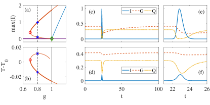
Figure 1: (Color online) (a,b) Branch of the single temporal LS as a function of the normalized gain $g$. We represent the maximum intensity (a) and the deviation of the period of the solution $T-T_{0}$. In (a) the blue line above threshold is the CW solution with minimal threshold, whose intensity was multiplied by $10^{2}$ for clarity. Temporal profiles for the stable solution (c) and the unstable branch (d). Other parameters are $\left(\alpha,\beta\right)=\left(0,0\right)$.

The spatial boundary condition due to the closing of a cavity onto itself after a propagation length $L$ appears as a time delay $\tau=L/c$ in Eq. (1). The latter governs the fundamental repetition rate of the PML laser. The lasing threshold $G_{th}$ is determined by the value of $G_{0}$ where the off solution $\left(A,G,Q\right)=\left(0,G_{0},Q_{0}\right)$ becomes linearly unstable. Above threshold, $G_{0}>G_{th}$, multiple monochromatic solutions $\left(A,G,Q\right)=\left(A_{k}e^{-i\omega_{k}t},G_{k},Q_{k}\right)$ exist VT-PRA-05 , with an amplitude $A_{k}$ and a frequency $\omega_{k}$ relative to the filter frequency. If $A_{k}\neq 0$, the modes are defined as the solutions of

$$\negthickspace\negthickspace\negthickspace\negthickspace\negthickspace 1-i\frac{\omega_{k}}{\gamma} = \sqrt{\kappa}\exp\left(\frac{\left(1-i\alpha\right)G-\left(1-i\beta\right)Q}{2}+i\omega_{k}\tau\right),$$ (4)

complemented with Eqs. (2-3) setting $\dot{G}=\dot{Q}=0$. Taking the modulus square of Eq. (4), we find the threshold condition with $A_{k}\rightarrow 0^{+}$,

$$G_{th}^{k} = Q_{0}+\ln\left[\frac{1+\left(\frac{\omega_{k}}{\gamma}\right)^{2}}{\kappa}\right]$$ (5)

while the modal frequency is given by the ratio of the real and imaginary parts and reads

$$\omega_{k}\tau -\left(\gamma\tau\right)\tan\left[\left(\alpha G_{th}-\beta Q_{0}\right)/2-\omega_{k}\tau\right]= 0.$$ (6)

In the long delay limit, one can safely assume that $\gamma\tau\gg 1$ and we can find a good approximation of the frequency of the mode with the lowest gain threshold $\omega_{0}$. Its expression reads simply

$$\omega_{0}\tau = \Theta$$ (7)

with $\Theta$ the material induced phase shift per round-trip $\Theta=\left(\alpha G_{0}-\beta Q_{0}\right)/2$. For this dominant mode, the threshold is $G_{th}^{0}=G_{th}=Q_{0}-\ln\kappa$.

Temporal LSs appear in TDSs in the long delay limit as periodic orbits whose period is always slightly larger than the time delay. This deviation is due to the inertia contained in the structure of a differential equation like Eq. (1). In our case, the physical interpretation of this reaction time is stemming from the finite bandwidth of the filter. The nominal period of the orbits in a PML laser described by Eqs. (1-3) is defined as $T_{0}=\tau+\gamma^{-1}$. The remaining deviation of the period with respect to $T_{0}$ results from the nonlinear contributions due to the dynamics of the gain and of the absorber and to phase-amplitude coupling. Finally we note that, as these temporal LSs are periodic orbits found in the long delay limit, they can be considered in principle as orbits approaching an homoclinic solution in the limit $\tau\rightarrow\infty$.

III Bifurcation analysis

(a)	(b)

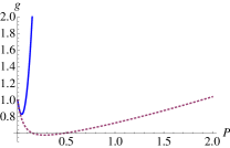
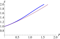
Figure 2: (Color online) Branch for the single pulse solution as a function of the normalized gain $g$ for strong (a) and weak (b) absorber nonlinearity. We represent the pulse energy as given by the weakly nonlinear analysis assuming a hyperbolic secant in blue, while the red dotted line is the result of a non-perturbative analysis, assuming a Dirac pulse shape. Only in the strong absorber regime in (a) $s=30$ and $Q_{0}=0.3$ we find a temporal LS bistable with the off solution while in (b) $s=5$ and $Q_{0}=0.01$, the pulse develops only above the lasing threshold. In this case a good agreement between the weakly nonlinear analysis and the non-perturbative analysis is found. Other parameters are $\alpha=\beta=0$.

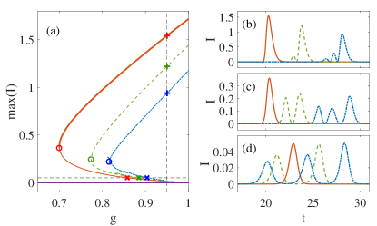
Figure 3: (Color online) (a) Multiple branches of temporal LSs as a function of the normalized gain $g$. In addition to the main branch appearing for the lowest values of the gain at $g_{SNL}^{\left(1\right)}=0.7$, other branches appear via additional SNL bifurcations at $g_{SNL}^{\left(2\right)}=0.774$, $g_{SNL}^{\left(3\right)}=0.816$, and consist in pulses composed of two or three maxima. The temporal profiles for the intensity are presented in panel (b-d), where, from top to bottom, we show the solutions on the upper branches (b) at $g=0.95$ (see vertical dashed line), the profiles at the saddle points (c), and those on the lower branch (d) with $\mathrm{max}\left(I\right)=0.05$ (see horizontal line). Other parameters are $\left(\alpha,\beta\right)=\left(0,0\right)$.

The main solution branch

We start by recalling the main characteristics of our temporal LSs setting $\alpha=\beta=0$. We operate in a regime of bistability in which, in addition to the stable off solution, two solutions that consist in temporal LSs exist. One is unstable and corresponds to a low intensity temporal pulse while the stable solution is the one of high intensity. The temporal LSs appear as a saddle-node bifurcation of limit cycle (SNL) below the lasing threshold, see Fig. 1(a), where we represented the maximal intensity of the pulse while Fig. 1(b) shows the deviation of the solution period $T-T_{0}$. We notice that the period of the stable portion of the branch is a decreasing function of $g$. As noted in JCM-PRL-16 ; CJM-PRA-16 , this results in repulsive interactions between temporal LSs as a gain depletion created by a LS will accelerate the next one away from it. We represent the temporal profile of the stable LS branch in Fig. 1(c), where the multiscale nature of the solution is apparent. While the optical pulse length is $\tau_{p}\sim 1$, the gain recovery is $3\tau_{g}\sim 75$. The inset Fig. 1(e) details the fast component of the LS. The unstable LS, that plays the role of a separatrix between the stable LS and the off solution, is represented in Fig. 1(d). We also show in Fig. 1(a) the dominant CW solution (the blue line). We stress that in our regime of localization the CW solutions are still supercritical and only develop above the lasing threshold. As such, we do not have bistability for the CW solution.

The typical pulse energy for the upper branch is $P\sim 1$, see Fig. 1(e), and $P\sim 0.1$ for the lower one, see Fig. 1(f). As such the absorber is operated in a strong saturation regime for which $sP\gg 1$. This regime is far beyond the reach of the usual hyperbolic secant ansatzes that allow finding values of the pulse energy and of the pulsewidth. Indeed, these hyperbolic secant ansatzes are correct only if the absorber saturation can be expanded up to second order, e.g. $\exp\left(-sP\right)\sim 1-sP+\left(sP\right)^{2}/2$. On the contrary, New’s approach of mode-locking N-JQE-74 only considers infinitely narrow pulses, e.g., Dirac deltas, but does not necessitate any approximation on the pulse energy. In our case, this second approach gives a much better agreement with exact numerics, although the details of the pulse shape and chirp cannot be obtained. The comparison of both approaches is depicted in Fig. 2 for the regime of strong and weak nonlinearities. The details of the calculations can be found in the appendix, for the simple case where $\alpha=\beta=0$. We notice that only in the strongly nonlinear regime one can obtain a sub-critical branch and bistability with the off solution. Also, only the beginning of the lower branch of solution is properly reproduced by the hyperbolic secant solution, since in this situation the pulse energy can be made arbitrarily small. While bistability is preserved by both approaches, neither the upper branch nor the folding point can be properly obtained using the hyperbolic secant ansatz. New’s approach is much more indicative for the extend of the bistable region and the pulse energy, if one compares with the results in Fig. 1 although it does not allow finding the details nor the possible instabilities of the temporal LSs. Finally, we note in Fig. 2(b) that for more standard parameters for PML, i.e., $s=5$ and $Q_{0}=0.01$, the pulsed solutions develops only above the lasing threshold an that in this case a good agreement between the weakly nonlinear analysis and the non-perturbative analysis is found. This comparison between the standard approaches of PML justifies the need for a detailed bifurcation analysis using path continuation techniques to fully study the localization regime.

Multi-peaked solutions

Still setting $\alpha=\beta=0$, we depict in Fig. 3(a) how, in addition to the main solution branch, additional solutions appear while increasing the bias current. We only present the first three branches bifurcating upon increasing $g$, yet additional solutions continue to appear at an increased rate when $g\rightarrow 1$. However, their evaluation becomes numerically tedious. We represent the temporal profiles of the intensity at $g=0.95$ on the upper part of the three branches in Fig. 3(b), at their respective folding points in Fig. 3(c), and on the lower part of the branches close to their appearance threshold, in Fig. 3(d). The low intensity branches are composed of LSs with an increasing number of bumps, similar to the molecules found for dissipative solitons systems, see e.g. GS-LNP-08 . Yet, the dynamics of the gain prevents, with parameters typical of semiconductors, the creation of stable molecules. As mentioned earlier, the gain dynamics induces a strong repulsion. All the multi-bump solutions evolve toward single pulse solutions when they reach the upper branch at high values of $g$.

Secondary Andronov-Hopf bifurcation

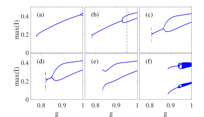
Figure 4: (Color online) (a-f) Stable branch of temporal LS as a function of the normalized gain $g$, obtained via direct numerical simulation of Eqs. (1-3). The dynamics are represented by the extrema of the time traces of the maximal pulse intensities. (a) $\alpha=3.7$, most of the branch is stable, although a secondary supercritical AH bifurcation is obtained for $g_{H_{1}}\simeq 0.98$. (b) For $\alpha=3.8$, the quasi-periodic regime shifts toward lower $g_{H_{1}}\simeq 0.92$ while another, subcritical, AH occurs at lower current $g_{H_{2}}\simeq 0.81$. (c) At $\alpha=4$ and (d) $\alpha=4.05$, the two quasi-periodic solutions come closer and finally merge at $\alpha=4.1$ as shown in (e). Higher values of $\alpha=5$ lead to a quasi-periodic cascade (f). Other parameters are $\beta=0.5$.

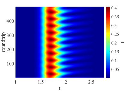
Figure 5: (Color online) Quasi-periodic limit cycle time trace obtained with $g=0.95$, see dotted line in Fig. 4(b), using a space-time representation. Other parameters are $\alpha=3.8$ and $\beta=0.5$.

We now turn our attention toward the dynamics found for large, yet realistic, values of the linewidth enhancement factors in the gain and the absorber sections. For the gain, we set $\alpha=3.7$ while for the absorber we set $\beta=0.5$. As the latter is operated below the transparency, the effects of band filling are much weaker, which justifies using a much smaller value of the Henry factor. As the bifurcation study of quasi-periodic orbits is not currently possible with ddebiftool, we performed direct numerical simulations of Eqs. (1-3). We integrated Eqs. (1-3) with a fourth order Runge-Kutta with Hermite interpolation of the time-delayed term and a step size $\Delta t=10^{-2}$. We depict in Fig. 4(a) the bifurcation diagram obtained by direct numerical integration, performing a parameter sweep in $g$, upward an downward starting from a central value. Using numerical integration, we can only show the upper part of the main branch, as it is the only stable solution. We observe that the main solution branch, that actually consists in a strongly nonlinear (pulsating) limit cycle, develops a secondary oscillation frequency (typically ranging between a few tens and a few hundreds of round-trips) when the gain is increased toward the lasing threshold. This slowly evolving orbit during which the pulse parameters are oscillating in time is depicted in Fig. 5 using a space-time representation for $\alpha=3.8$. Here, we show the evolution of the pulse train, from one round-trip to the next. This diagram allows us to identify this secondary Andronov-Hopf (AH) instability as a trailing edge instability. As it occurs for large values of $\alpha$ and increasing values of the gain, we posit it is a dispersive (phase) instability.

The evolution of this emerging limit cycle is depicted in Fig. 4(c) for higher values of $\alpha=4$ which shifts the secondary AH to lower values of $g$ while another subcritical AH appears at a lower value of the gain. In this regime, the region of stable operation is delimited by these two AH bifurcations. Using higher values of $\alpha=4.1$ leads to a collision and a merging of these two quasi-periodic solutions, see Fig. 4(d,e). In this regime, stable LSs do not exist and solely oscillating quasi-periodic solutions are found. For larger values of $\alpha$ and high gain, a typical transition to irregular dynamics via quasi-periodicity is observed, which is visible in Fig. 4(f) where the maximal pulse intensity shows quasi-continuous values.

In order to understand how the various regimes are connected together, we performed a double scan in the parameters $\alpha$ and $g$. Our results are summarized in Fig. 6. We superposed to these numerical results the evolution of the SNL point for the primary branch as well as the secondary AH point found by using ddebiftool, finding a good agreement. While ddebiftool cannot track the emerging solution, it can identifies the secondary AH point, which is actually a Neimark-Sacker bifurcation. First, we note in Fig. 6(a) that the SNL values depend rather weakly on $\alpha$ and that the minimal value of $g_{SNL}$ is not attained for $\alpha=0$. This is due to the presence of a non-zero value of $\beta$ and a small value of $\alpha$ can compensate for the chirp created by the absorber. However, the Lorentzian filter in Eq. (1) limits the optical bandwidth of the field and high values of $\alpha$ induce additional chirp for the pulses which, in turn, creates additional optical bandwidth that gets absorbed by the filter. As such, highly chirped pulses experience more losses and can not exist for too low values of the gain, which explains why the SNL point increases in $g$ for large values of $\alpha$. Also, one notices a different scenario depending on the value of $\alpha$. For low values of $\alpha$ an extended domain of stability ranges from the appearance of the SNL bifurcation for low $g=g_{SNL}$ toward threshold $g=1$. For higher values of $\alpha\in\left[3.7,3.75\right]$, the solution stability is still governed by the SNL for low values of $g$ but by the AH bifurcation that is crossed at higher values of $g$. We notice that the two AH bifurcations depicted in Fig. 4(b-d) are actually stemming from the same AH curve in the $\left(g,\alpha\right)$ plane that can be crossed twice upon increasing $g$. For higher values of $\alpha\in\left[3.75,4.1\right]$, the stable domain for the LS is enclosed between the two AH points. For values of $\alpha>4.1$, where the two AH points merged, the only kind of LS that exists is an oscillating one.

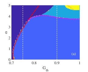
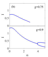
Figure 6: (Color online) (a) Two dimensional bifurcation diagram as a function of $g$ and $\alpha$. Dark blue: off solution. Blue: stable LS, light blue: periodically oscillating. Yellow: quasi-periodic LS oscillation. (b) Vertical cuts of the diagram in (a) obtained for $g_{1}=0.75$ and $g_{2}=0.9$ as a function of $\alpha$. One notices for low values of $\alpha$ an extended domain of stability ranging from the appearance of the SNL bifurcation for low $g$ toward threshold $g=1$. We superposed the results obtained with ddebiftool where the red dash-dotted and pink dashed lines correspond to the SNL and the secondary AH, respectively. Other parameters are $\beta=0.5$.

Similar diagrams were obtained for other values of parameters, and we note that, while it is not the case with $\beta=0.5$, some bistability between steady and oscillating solutions could be observed in a finite interval of $\left(g,\alpha\right)$ by setting $\beta=0$. It stands to reason that this bistability could be preserved for low values of $\beta$ and adapted values of the other parameters as, e.g., $\left(\kappa,q_{0},s\right)$.

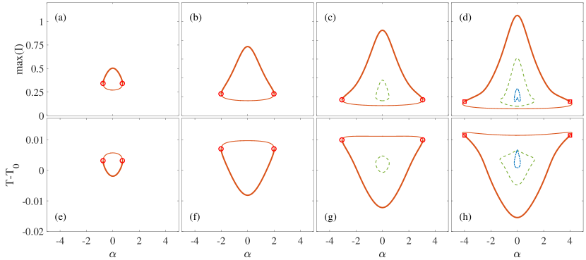
Figure 7: (Color online) (a) Two-dimensional bifurcation diagram in $\alpha$ for increasing values of $g$. We represent the maximum intensity (a-d) and the period deviation (e-h). The value of the gain is $g=0.707$ (a,e), $g=0.745$ (b,f), $g=0.784$ (c,g) and $g=0.822$ (d,h). Stability is indicated with thick lines. Additional solution loops are born via saddle-node bifurcations upon increasing $g$. Other parameters are $\beta=0$.

Organization of solutions in the $\left(g,\alpha\right)$ plane

We now turn our attention to how the multiple solution branches depicted in Fig. 3 organize by making a three-dimensional bifurcation diagram of the LS solutions where our control parameters are $\left(\alpha,g\right)$. First, we set the linewidth enhancement factor of the absorber to $\beta=0$. Our results are summarized in Fig. 7, where we present various slices of the diagram, the solution curves in $\alpha$, for increasing values of $g$. We represent the maximum pulse intensity as well as the period deviation of the solution. As we want to emphasize the solution structure, we extended our analysis to negative values of $\alpha$. For $\beta=0$, the diagram is perfectly symmetrical, since negative values of $\alpha$ simply consist in taking the complex conjugate of Eq. (1). Firstly, we note in Fig. 7(a,e) that the solution loop folds for larger values of $\alpha$, here $\alpha_{fold}\sim\pm 1$. As previously mentioned, $\alpha$ induces additional chirp of the solution which limits the region of existence of the LSs. A higher value of $g$ depicted in Fig. 7(b,f) allows the LS solution to exists at higher values of $\alpha$. This evolution of the folding point is another representation of the evolution of the SNL curve shown in Fig. 6. One notices that the solution structure, at low $g$, resembles a paraboloid growing in radius when $g$ is increased, that then deforms nonlinearly. At higher values of $g$, an additional solution loop emerges, see Fig. 7(c,g). This loop corresponds to the solutions with a double pulse, and it grows in radius at higher $g$, see Fig. 7(d,g), where also a third loop with a three peaked solution emerges.

We depict the interaction occurring between these various solution loops when they become of comparable amplitude. The interactions between the primary and the secondary loops is described in Fig. 8. For $g=0.879$, the outer branch, that is the stable solution for large $\alpha$, develops a pair of folds via a cusp bifurcation. This cusp takes the form of an additional loop along the branch, if one represents the maximum pulse intensity, see the inset in Fig. 8(c). For $g=0.898$, the primary and secondary solution loops have crossed each other via a transcritical bifurcation. This mechanism is important because, at high values $\alpha$, it is now the secondary branch, initially unstable and showing solutions with two peaks, that is responsible of giving the stable solution with a single peak, see Fig. 8(b) and the inset in Fig. 8(d). As previously mentioned, the mechanism by which the two solution loops can cross is a transcritical bifurcation. We depict this mechanism by which the solution curves are allowed to cross each other in a small vicinity of the bifurcation point in Fig. 9.

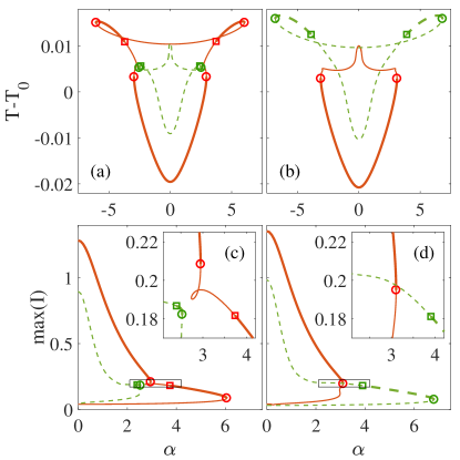
Figure 8: (Color online) (a-d) Bifurcation diagrams as a function of $\alpha$ for two close-by values of the gain, $g=0.879$ (a,c) and $g=0.898$ (b,d). We represent in (a,b) the deviation of the period and the maximum intensity in (c,d). Stable solutions are depicted in thick lines. Open circles denote the fold positions whereas squares indicate the AH bifurcation points. Other parameters are $\beta=0$.

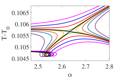
Figure 9: (Color online) (a) Zoom around the transcritical bifurcation depicted in Fig. 8. The deviation of the period is shown. The values of $g$ are interspersed in the interval $g\in\left[0.8793;0.8812\right]$. Other parameters are $\beta=0$.

Finally, we consider how to this bifurcation scenario changes when $\beta\neq 0$. We set $\beta=0.5$ and the first consequence of having $\beta\neq 0$ is that the symmetry $\alpha\rightarrow-\alpha$ of the bifurcation diagrams depicted in Fig. 7 is broken. While for $\beta=0$ pairs of transcritical bifurcations would appear symmetrically and reconnect parts of some solution loops with others on both sides, it is not the case anymore. Our results are depicted in Fig. 10 where we can appreciate the changes in the bifurcation scenario. While the gradual appearance of additional solutions is preserved when increasing $g$, see Fig. 10(a,e), we notice that the transcritical bifurcations appear in an alternated way, first for a negative value of $\alpha$, see Fig. 10(b,f), then for a positive, yet different value of $\alpha$, see Fig. 10(d,h). This has the consequence of giving the solution surface the visual appearance of a Klein bottle, as depicted for instance in Fig. 10(c,g). Here, the apparent self-intersection of the primary solution branch is visible. However, while the branch seems to self-intersect when looking at the maximum pulse intensity, another measure of the branch would give a different representation.

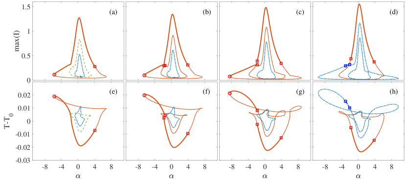
Figure 10: (Color online) (a) Two-dimensional bifurcation diagram in $\alpha$ for increasing values of $g$. We represent the maximum intensity (a-d) and the period deviation (e-h). The value of the gain is $g=0.879$ (a,e), $g=0.898$ (b,f), $g=0.937$ (c,g) and $g=0.956$ (d,h). Stability is indicated with thick lines. Open circles denote the fold positions whereas squares indicate the AH bifurcation points. The different branches intersect asymmetrically when increasing $g$ at $\beta=0.5$.

IV The exponential Haus master equation

In this section, we turn our attention toward the predictions given by a different approach that is based upon a partial differential equation (PDE) instead of a DDE. This modified Haus master equation considers the evolution of a pulse on a slow time scale that corresponds to the number of round-trips in the cavity. As such, this iterative pulse mapping can be much more efficient computationally. In addition, while the LSs are periodic solutions of a DDE, they become steady states of a one-dimensional PDE, which can lead to further bifurcation analysis. For instance, the branches of periodic solutions of a PDE can be computed using the path continuation methods while the quasi-periodic solutions of the DDE cannot be evaluated with ddebiftool at the moment. Another argument that makes the PDE approach appealing. One can actually restrict the numerical domain along the propagation axis to a box that is a few times the extension of the optical pulse. That way, the long gain recovery, during which the field is zero can be discarded, which results in a much reduced number of degree of freedom during the continuation.

We outline how the DDE given by Eqs. (1-3) can be recast into a PDE. We have seen that, at the lasing threshold, the maximum gain mode needs to have a frequency shift $\omega_{0}=\Theta/\tau$. While the frequency shift is arbitrarily small in the long delay limit, the phase shift per pass $\Theta$ is not. It is essential, as it compensates for the index variation created by the active medium after one round-trip. Within the framework of an iterative pulse model as the Haus master equation, that does not contain anymore proper boundary conditions for the field, this frequency shift has to be canceled out before making the correspondence between the DDE and the PDE. We perform the change of variable $A\left(t\right)=E\left(t\right)e^{-i\omega_{0}t}$ in order to cancel this rotation, which leads to the modified field equation

$$\frac{\dot{E}}{\gamma}-i\frac{\Theta}{\gamma\tau}E = R_{\tau}e^{i\Theta}E_{\tau}-E,$$ (8)

while the carrier equations are identical simply setting $A\rightarrow E$. Following the method depicted in CJM-PRA-16 , the Eqs. (8,2,3) can be transformed into a PDE, taking advantage of the long cavity limit at which we operate this system experimentally. We do not repeat the procedure that can be found in CJM-PRA-16 and only sketch the reasoning. We start by defining a smallness parameter as the inverse of the filter bandwidth setting $\varepsilon=1/\gamma$. Physical intuition dictates that the pulse-width scales as the inverse of the filter bandwidth and that it is proportional to $\gamma^{-1}=\varepsilon$. This intuition is confirmed by the numerical continuation. In a related way, one can foresee that the period of the pulse train scales as $T_{0}\sim\tau+\gamma^{-1}$, i.e., the period is always larger than the delay due to causality and the finite response time of the filtering element that limit the optical bandwidth available. As such, we assume that the solution is composed of two time scales and write

$$\frac{d}{dt} \rightarrow \frac{\partial}{\partial z}+\varepsilon^{2}\frac{\partial}{\partial s}$$ (9)

with $\left(z\right)$ governing the fast evolution along the cavity axis and $s$ depicting the slow dynamics after each round-trip. Following GP-PRL-96 , we express the delayed term as

$$E\left(t+\tau\right) = E\left(z+\varepsilon\upsilon,s+\varepsilon^{2}\tau\right),$$ (10)

which means that the solution after one round-trip is slowly evolving and drifting. Upon expanding all contributions up to $\mathcal{O}\left(\varepsilon^{3}\right)$, one finds that the drift term can be canceled setting $\upsilon=-1$. In other words, the solution at the next round-trip is shifted to the right, which precisely corresponds to a period of $T_{0}=\tau+\gamma^{-1}$. Finally, defining a time scale normalized by the round-trip as $\sigma=s/\varepsilon^{2}\tau$ and setting $I=\left|E\right|^{2}$ we find

$$\frac{\partial E}{\partial\sigma}-\frac{1}{2\gamma^{2}}\frac{\partial^{2}E}{\partial z^{2}} =$$

$$\left(\sqrt{\kappa}e^{\frac{1-i\alpha}{2}G-\frac{1-i\beta}{2}Q+i\Theta}-1+i\frac{\Theta}{\gamma\tau}\right)E,$$

$$\frac{\partial G}{\partial z}+\frac{1}{\tau}\frac{\partial G}{\partial\sigma} = \Gamma\left(G_{0}-G\right)-e^{-Q}\left(e^{G}-1\right)I,$$ (12)

$$\frac{\partial Q}{\partial z}+\frac{1}{\tau}\frac{\partial Q}{\partial\sigma} = Q_{0}-Q-s\left(1-e^{-Q}\right)I.$$ (13)

We can now invoke the long delay limit and discard in Eq. (IV-13), all the contributions that are proportional to $1/\tau$. Note that while the contribution $\Theta/\left(\gamma\tau\right)$ is irrelevant, we must keep the term $\exp\left(i\Theta\right)$ in Eq. (IV). Hence, we obtain the following PDE system

$$\frac{\partial E}{\partial\sigma}-\frac{1}{2\gamma^{2}}\frac{\partial^{2}E}{\partial z^{2}} = \left(\sqrt{\kappa}e^{\frac{1-i\alpha}{2}G-\frac{1-i\beta}{2}Q+i\Theta}-1\right)E,$$ (14)

$$\frac{\partial G}{\partial z} = \Gamma\left(G_{0}-G\right)-e^{-Q}\left(e^{G}-1\right)I,$$ (15)

$$\frac{\partial Q}{\partial z} = Q_{0}-Q-s\left(1-e^{-Q}\right)I.$$ (16)

The Eqs. (14-16) can be understood as a generalization of the Haus master equation to large gain and absorption per pass. Indeed, one of the main advantages of the model of VT-PRA-05 is the consideration of large gain and absorption per round-trip, a feature that is still preserved by the exponential terms in Eqs. (14-16). The longitudinal variable $\left(z\right)$ identifies as a fast time variable and represents the longitudinal evolution of the field within the round-trip. From the inspection of Eqs. (12,13) one can clearly see that the parity symmetry $\left(z\right)\rightarrow\left(-z\right)$, is being broken by the carrier dynamics that is only first order in $\partial_{z}$, a symmetry is only recovered upon making the adiabatic elimination of $G$ and $Q$. Notice that while the regime of a fast absorber is a meaningful limit, the gain is the slowest variable and it cannot be eliminated by taking the long cavity limit.

V Bifurcation Analysis of the Exponential Haus Equation

In this section we present the bifurcation analysis of the generalized Haus master equation described by Eqs. (14-16) and discuss how it is related to that of the DDE model given by Eqs. (1-3). The temporal LS solutions of Eqs. (14-16) are slowly drifting oscillating solutions that can be found as steady states of Eqs. (14-16) by setting

$$E\left(z,\sigma\right) = E\left(z-\upsilon\sigma,\sigma\right)\exp\left(-i\omega\sigma\right)$$ (17)

which adds a contribution $\left(\upsilon\partial_{z}+i\omega\right)E$ to the right hand side of Eq. (14). We recall that the steady states of Eqs. (14-16) are actually the periodic solutions of Eqs. (1-3). We followed the LS solutions of Eqs. (14,16) in parameter space, by using pseudo-arclength continuation within the pde2path framework uecker2014 .

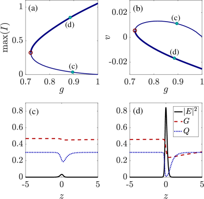
Figure 11: (Color online) (a,b) Branch of the single temporal LS as a function of the normalized gain $g$ calculated for $(\alpha,\text{\,$\beta$})=(1.5,\,0.5)$. We represent (a) the maximum intensity and (b) the drift velocity $\upsilon$. The LS is stable beyond the saddle-node bifurcation point $g_{SN}=0.721$ (red circle). (c,d) Two exemplary stationary LS profiles for the unstable branch (c) and the stable one (d) for $g=0.896$ and $g=0.886$, respectively. Other parameters are $(\gamma,\,\kappa,\,\Gamma,\,Q_{0},\,s)=\left(10,\,0.8,\,0.04,\,0.3,\,30\right)$.

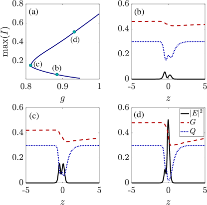
Figure 12: (Color online) (a) Branch for the two-peaked LS solution obtained for $(\alpha,\,\beta)=(1.5,\,0.5)$ as a function of the normalized gain $g$ where we represent the maximum intensity. Temporal profiles for the low intensity solution (b) at $g_{b}=0.885$, the solution at the fold $g_{c}=0.813$ (c) and on the upper branch (d) at $g_{d}=0.932$. The whole solution branch is unstable. Other parameters are the same as in Fig. 11.

In our case, the primary continuation parameter is, e.g., the gain parameter $g$ or the linewidth enhancement factor $\alpha$. However, the spectral parameter $\omega$ and the drift velocity $\upsilon$ become two additional free parameters that are automatically adapted during the continuation. In order to determine $\left(\omega,\upsilon\right)$, we impose additional auxiliary conditions. In particular, we set the solution speed, defining $u\left(z,\sigma\right)=\left[\Re\left(E\right),\,\Im\left(E\right),\,G,\,Q\right]$, by using the integral phase condition

$$\int u\cdot\frac{\partial u_{\mathrm{old}}}{\partial z}dz = 0,$$ (18)

where $u_{\mathrm{old}}$ denotes the solution obtained in the previous continuation step. Further, one needs an additional auxiliary condition to break the phase shift symmetry of the system in order to prevent the continuation algorithm to trivially follow solutions along the corresponding neutral degree of freedom. This condition can be easily implemented by, e.g., setting the phase of the LS to zero in the center of the computational domain. This condition allows finding the value of $\omega$ and reads

$$\Im\left[E\left(\frac{L}{2}\right)\right] = 0.$$ (19)

To increase computational efficiency, we used a domain whose length $L$ is much smaller than the recovery time of the gain and set $L=10$. In addition, we impose no-flux boundary conditions on both ends of the numerical domain

$$\frac{du}{dz}\left(0\right)=\frac{du}{dz}\left(L\right)=0,$$ (20)

while the number of mesh points is $N=512$. We note that other kinds of boundary conditions as, e.g., setting $E\left(0\right)=E\left(L\right)=0$ gave very similar results. Notice that in the case where the domain is sufficiently large so that if the field intensity is zero, the proper conditions for $G$ and $Q$ are of the Robin type and are simply Eqs. (15-16) setting $E=0$

$$\frac{\partial G}{\partial z}+\Gamma G = \Gamma G_{0}\,\quad\quad\frac{\partial Q}{\partial z}+Q=Q_{0}.$$ (21)

Now one can start at, e.g., a numerically given solution, continue it in parameter space, and obtain a LS solution branch. The result is depicted in Fig. 11, where the evolution of (a) the (peak) intensity $I$ and (b) the drifting speed $\upsilon$ as a function of the normalized gain $g$ is presented. We observe that the main branch of the temporal LS bifurcates from $g=g_{th}=1$, possesses a fold at some fixed value $g_{SN}$ (marked as the red circle in Fig. 11) and goes to higher intensities. Note that in the case of Eqs. (14-16), the solution appears upon increasing $g$ as a saddle-node bifurcation (SN) and not a saddle-node of limit cycle (SNL) as for Eqs. (1-3). The critical value is $g_{SN}=0.721$ which compares very well with the results of the DDE model for which we have $g_{SNL}=0.716$. We note that the drifting speed $\upsilon$ is a decreasing function of $g$ for the stable branch of the solution. This result is in good agreement with the solutions of Eqs. (1-3) because the drift velocity can be identified with the deviation of the period with respect to $T_{0}$, per unit of $\tau,$ hence the corresponding transformation is $\upsilon=\left(T-T_{0}\right)$. Further, in Fig. 11 (c,d) we show two exemplary stationary LS profiles that exist for different values of $g$. One can see that the peak intensity of the LS changes significantly along the branch, leading to the formation of a narrow peak of high intensity at the upper branch part.

The Haus PDE (14-16) also predicts the existence of additional branches of solutions that are composed of several peaks. We depict in Fig. 12 the secondary branch of two-peaked solutions. Here, a double peak LS emerges at low intensities and folds back at $g_{SN}^{\left(2\right)}=0.813$ which compares very well with $g_{SNL}^{\left(2\right)}=0.808$ given by the DDE model. In addition, in Fig. 12 (b-d) we depict three exemplary LS profiles that exist for different values of $g$. As in the case of the DDE model (cf. Fig. 3), the low intensity branch is composed of two-bumps solutions of different heights and evolve toward a single bump solution for high values of $g$ at the upper branch part. For the third branch, we were not able to find a proper starting solution, as the whole branch is unstable, which, however, does not mean the three-peaked solution does not exist in Eqs. (14-16).

In addition to stationary LS solutions, Eqs. (14-16) also predict the existence of temporally oscillating solutions. We start their analysis with the case where the line enhancement factor of the absorber $\beta=0$ and perform a continuation in $\alpha$. There, the branches with different numbers of peaks emerge and reconnect via the same scenario as in the DDE model (1-3) involving transcritical bifurcations (cf. Fig. 8) although it is much more difficult to obtain such results within the PDE continuation. An example of the resulting branch structure for $g=0.955$ is depicted in Fig. 13, where the branches of the primary (red) and secondary (cyan) solutions are shown after the re-connection.

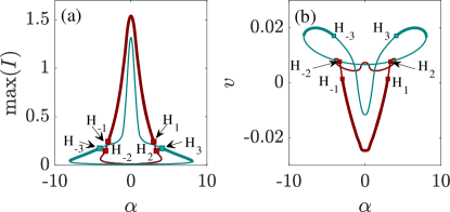
Figure 13: (Color online) A bifurcation diagram as a function of $\alpha$ obtained for $\beta=0$ at a fixed value of the gain $g=0.955$. We represent (a) the maximum intensity as well as (b) the drifting speed of the solution $\upsilon$. Stability is indicated with thick lines: On the main branch (red) the LS is stable between the AH points $\mathrm{H_{\pm 1}}$, the secondary AH bifurcations are indicated as $\mathrm{H_{\pm 2}}$. The LS on the secondary branch (cyan) is stable between the AH points $\mathrm{H_{\pm 3}}$ and the folds. Other parameters are the same as in Fig. 11.

One can see that on the main branch the LS is stable between the symmetrically situated AH bifurcation points $\mathrm{H_{\pm 1}}$, whereas the secondary AH bifurcations appear at $\mathrm{H_{\pm 2}}$. Further, the LS solution on the secondary branch becomes stable for the high $\alpha$ values between the AH points $\mathrm{H_{\pm 3}}$ and the corresponding folds, which is again in agreement with the DDE results (cf. Fig. 8). In addition, in Fig. 14 we show a space-time representation of the intensity field evolution obtained by direct numerical simulations of Eqs. (14-16) for two different values of $\alpha$ close to the AH bifurcation points $\mathrm{H_{1}}$, $\mathrm{H_{3}}$ keeping the other parameters fixed. For the numerical integration of the model in question a Fourier based semi-implicit split-step method is employed, see the appendix of GJ-PRA-17 . Our results reveal that indeed two AH bifurcations can be found for different values of $\alpha$ that co-exist at a fixed value of $g$.

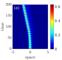
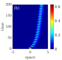
Figure 14: (Color online) Space-time representation of the intensity field of AH unstable solutions obtained from direct numerical simulations of the model (14-16) for different values of $\alpha$ at fixed $g=0.955$ and $\beta=0$ (cf. Fig. 13). Parameters are chosen to be close to the AH points $\mathrm{H_{1}}$(a) $\alpha=2.8$ and $\mathrm{H_{3}}$ (b) $\alpha=3.6$. Other parameters are the same as in Fig. 11.

As in the case of the DDE model, for $\beta=0$ the resulting branches are perfectly symmetrical. However, when $\beta\neq 0$ the symmetry of the diagram is broken and one does see how the solution curves deform when the gain is increased in Fig. 15. Here, the evolution of the peak intensity (a) and the drifting velocity (b) of the main solution branch are presented for $\beta=0.5$. Stability of the LS solution is indicated with thick lines, whereas cyan squares mark the positions of appearing AH bifurcations. At variance with ddebiftool, for the PDE model (14-16) we have an access to the critical eigenfunctions of the system that inform on the particular shape of the waveform. An example of the real parts of the first two components of the critical eigenfunction $\psi=[\psi_{1},\psi_{2},\psi_{3},\psi_{4}]$ associated with the AH instability (dashed red lines) are shown together with the corresponding $(\Re(E),\,\Im(E))$ components of the field (solid black lines) in Fig. 16. Here, the parameters are chosen to be close to the AH bifurcation point at the red line of Fig. 15, corresponding to $g=0.94$. It turns out that the components of the unstable eigenfunction are localized on the trailing edge of the field components. That is, the branch of the LS gets destabilized via oscillations, localized on the trailing edge of the LS (cf. Fig. 14).

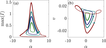
Figure 15: (Color online) Two-dimensional bifurcation diagram in $\alpha$ for $\beta=0.5$ when increasing the gain $g$. We represent the maximum intensity of the main LS solution (a) as well as its the drifting speed $\upsilon$ (b). The values of the gain are $g=0.73$ (green), $g=0.78$ (blue), $g=0.83$ (cyan) and $g=0.94$ (red). Stability is indicated with thick lines, whereas cyan squares indicate the positions of the AH bifurcation. Other parameters are the same as in Fig. 11.

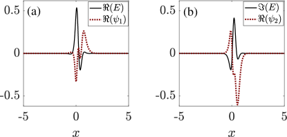
Figure 16: (Color online) Real parts of the first two components of the critical eigenfunction $\psi$ of the Hopf unstable solution (red dashed lines) together with the $(\Re(E),\Im(E))$ components of the field (black solid lines). Parameters are $\left(g,\alpha,\beta\right)=\left(0.94,4.179,0.5\right)$ (cf. Fig. 15). Other parameters are the same as in Fig. 11.

Interestingly, we can also show how the AH bifurcation can be inhibited or activated by considering the influence of group velocity dispersion (GVD). We note that, while this analysis is direct within the framework of the modified Haus equation, and simply consists in adding an imaginary contribution to the second order derivative in $z$ in Eq. (14) $+iD\partial_{z}^{2}E$, it is not directly possible to do the same transformation with the DDE model. Adding some amount of dispersion in a DDE model can only be done via a much more involved method PSH-PRL-17 . We note that the dispersion coefficient $D$ corresponds to $D=-\beta_{2}/\tau$ with $\beta_{2}$ the chromatic dispersion. As such $D>0$ corresponds to anomalous dispersion which favors, e.g., with a self-focusing nonlinearity $\sim+i\left|E\right|^{2}E$, the appearance of bright solitons. In our case, however, the effect of GVD is more complex than for the case of weakly dissipative solitons because the nonlinearity can be either focusing or defocusing depending on the values of $\alpha$ and $\beta$. In addition the nonlinearity is mediated by two dynamical variables having very different time scales. To illustrate the influence of GVD on the LS behavior we show in Fig. 17 the evolution of the main solution branch in $g$ for two different values of $\alpha$ and three different values of $D$. Here, we represent the maximum intensity (a,c) and the spectral parameter $\omega$ (b,d). We notice in Fig. 17(a-b) for $\alpha=4.5$ that the solution is stable beyond the AH bifurcation (cf. thick lines). This AH point actually corresponds to the first, subcritical, secondary AH bifurcation depicted in Fig. 6 below which the oscillation rapidly explodes nonlinearly. Here the effect of positive GVD is to inhibit the AH bifurcation. Some amount of anomalous dispersion favors the existence of the temporal LSs as it pushes the secondary AH bifurcation to higher values of $g$, resulting in an extended range of stability in Fig. 17(a,b). Yet, this scenario is changed for slightly smaller value of $\alpha=4.3$, where one can see that the effect of GVD is inverse and favors the secondary AH for $D>0$ while inhibits it for $D<0$. From this analysis we can draw the conclusion that while the main branch characteristics such as the folding point, intensity and pulse shape are well reproduced by the exponential Haus master equation, the scenario for the secondary AH bifurcation is affected. In particular, while we do see the emergence of the subcritical AH bifurcation, the supercritical AH is absent. This difference can be ascribed to the fact that the carrier frequency of the solution $\omega$ oscillates in time leading to a delayed phase $\omega\tau$ that is slowly evolving, a feature lost in the PDE mapping presented in Eqs. (14-16).

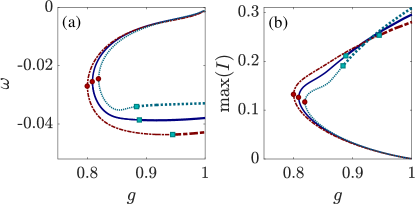
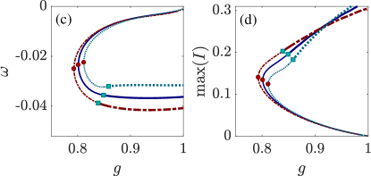
Figure 17: (Color online) Main solution branch as a function of the normalized gain $g$ for different amounts of the GVD parameter $D$ and different values of $\alpha$ at fixed $\beta=0.5$. (a,b) $\alpha=4.5$ and (c,d) $\alpha=4.3$. We represent the maximum intensity (a,c) and the frequency shift $\omega$ (b,d). The different curves correspond to $D=-10^{-3}$ (dash-dotted red), $D=0$ (solid blue) and $D=10^{-3}$(dotted cyan). The corresponding saddle-nodes (red circles) in (a,b) are located at $g_{SN}=[0.80,\,0.808,\,0.819]$, while the AH bifurcation positions (cyan squares) are $g_{AH}=[0.944,\,0.888,\,0.883]$. In (c,d) the saddle-nodes (red circles) are located at $g_{SN}=[0.793,\,0.801,\,0.811]$, while the AH bifurcation positions (cyan squares) are $g_{AH}=[0.839,\,0.849,\,0.858]$. Other parameters are the same as in Fig. 11.

Finally, we depict the summary of our bifurcation analysis of both the DDE and the PDE models in Fig. 18 allowing for a more direct global comparison. Here we represent the bifurcation diagram in the $(g,\,\alpha)$ plane, showing the SNL points of the DDE for both the primary (red dashed line) and the secondary (solid blue line) branches, and compared it with the SN points of the PDE (green circles), as well as the the secondary AH bifurcation occurring on the primary branch in the DDE (pink dotted line) in addition to the primary AH of the PDE model (cyan crosses). Here, the appearance of the cups is visible for both models. We do notice a small deviation for the folding point of the solution while the secondary Andronov-Hopf lines are significantly different. While the AH lines grows and falls as a function of $g$ in the DDE case, the one in the PDE model is steadily increasing, which explains the difference encountered in Fig. 17. While scanning $g$ in the DDE model, one can cross twice the AH line, giving rise to the sub- and supercritical limit cycles depicted, e.g., in Fig. 4(c,d), the line can only be crossed once in the PDE model, giving rise only to the subcritical limit cycle. Finally, it was not possible to follow the cusp bifurcation on the secondary branch in the PDE model for all values of $g$, although we believe that it would closely follow the same trend as in the DDE model.

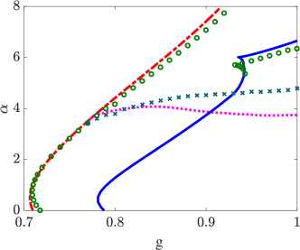
Figure 18: (Color online) Bifurcation diagram in the $\left(g,\alpha\right)$ plane, showing the evolution of the bifurcation points of both DDE and PDE models . The primary SNL bifurcation (dotted red line) of the DDE defines the breadth of the paraboloid for the primary solution. The secondary SNL is depicted in solid blue and the cusp is visible around $g=0.935$. The secondary AH bifurcation is depicted in dotted pink and it connects with the SNL on a codimension two point. The SN points of the PDE are shown as green circles, whereas cyan crosses stay for the primary AH points. The cusp for the PDE is around $g=0.932.$ Other parameters are $\beta=0.5$.

VI Conclusion

In conclusion, we discussed the bifurcation and the stability analysis of the time periodic solutions of the PML laser found in the long delay limit. We demonstrated that besides the main solution branch disclosed in MJB-PRL-14 , numerous additional branches exist, and that upon increasing the bias current, they splice with the main solution loop via transcritical bifurcations leading to a seemingly self-intersecting manifold for the solutions. We showed that for large but realistic values of the $\alpha$-factor in the gain section, the secondary branch is an essential part of the bifurcation scenario as it is the one giving the stable solution for large gain. A secondary Andronov-Hopf (AH) bifurcation is found either increasing the gain or the $\alpha$ factor leading to slowly evolving oscillations of the LS waveform. As the destabilization is found for increasing $\alpha$ factor, this points toward a dispersive nature of this instability. In addition, the bifurcation analysis of the modified Haus equation is presented. We showed that this model needs to consider an additional phase factor in order to properly reproduce the lasing threshold. A good agreement was found, not only for a single time trace, but for the whole bifurcation diagram, although the analysis with pde2path proved to be more technically involved. It was shown that the Andronov-Hopf instability found for large $\alpha$-values can be mitigated by introducing some amount of group velocity dispersion which counteracts the dispersive effect induced by the material. Our preliminary study indicated that GVD may have a profound impact on the dynamics of temporal LSs. Notice that introducing GVD at the level of the Haus PDE is direct while it is known to be quite challenging in the DDE approach.

While we found a good agreement for the bifurcation diagram explaining the emergence of the single LS, we found some discrepancies regarding the secondary instabilities. In particular, the evolution of the secondary AH line in the $\left(g,\alpha\right)$ plane was found to be significantly different, leading to a quantitatively different bifurcation scenario for values of $\alpha$ in a particular interval: While the AH line could be crossed twice in the DDE model, it is only crossed once in the “equivalent” PDE. However, this discrepancy was found to occur only in a small interval of the linewidth enhancement factor of the gain section. Overall we demonstrated in this manuscript that, while the coherent modal structure of the DDE is lost due to the absence of boundary conditions and the secondary AH regime can be shifted, the exponential Haus master equation can be considered as an effective order parameter equation representing the dynamics of a temporal LS found in the DDE model. The good agreement between the two approaches validates further studies regarding the effect of GVD on temporal LSs, but also on light bullets.

Appendix

Analytical solutions for the pulse shape in the subcritical region below threshold can only be found in the so-called Uniform Field Limit (UFL) where the gain, absorption and losses are small at each round-trip. We note that these approximations mean that $G$ and $Q$ are small, but their responses are not necessarily weakly nonlinear in the field intensity. The UFL consists in linearizing the gain and absorption per pass in Eqs. (14-16), setting $e^{G}=1+G$ and $e^{-Q}=1-Q$. This approximation will allow us to factor out the cavity losses. To do, so we define the new expression of the threshold in this linearized model as

$$G_{th} = Q_{0}+2\frac{1-\sqrt{\kappa}}{\sqrt{\kappa}}\,.$$ (22)

We also defined the normalized absorption as

$$q = \frac{\sqrt{\kappa}Q}{2\left(1-\sqrt{\kappa}\right)}$$ (23)

and as such, $g=G/G_{th}$, $g_{0}=G_{0}/G_{th}$ and $q_{0}=\sqrt{\kappa}Q_{0}/\left[2\left(1-\sqrt{\kappa}\right)\right]$ leading to

$$G_{0} = 2g_{0}\frac{1-\sqrt{\kappa}}{\sqrt{\kappa}}\left(q_{0}+1\right)\,.$$

Replacing these expressions into the linearized Eq. (14), we find the following,

$$\frac{\partial E}{\partial\tilde{\sigma}}-\frac{1}{2\tilde{\gamma}^{2}}\frac{\partial^{2}E}{\partial z^{2}} = \left[\left(1-i\alpha\right)\left(q_{0}+1\right)g-\right.$$

$$\left.-\left(1-i\beta\right)q-1+i\theta\right]E,$$

$$\frac{\partial g}{\partial z} = \Gamma\left(g_{0}-g\right)-g\left|E\right|^{2},$$ (25)

$$\frac{\partial q}{\partial z} = q_{0}-q-qs\left|E\right|^{2},$$ (26)

where we normalized the slow time as $\tilde{\sigma}=\left(1-\sqrt{\kappa}\right)\sigma$, the filter bandwidth $\tilde{\gamma}=\sqrt{1-\sqrt{\kappa}}$$\gamma$ and the phase $\Theta$ as $\theta=\Theta\sqrt{\kappa}/\left(1-\sqrt{\kappa}\right)$ hence $\theta=\alpha\left(q_{0}+1\right)g_{0}-\beta q_{0}$. In Eqs. (Appendix-26), the parameter $\kappa$ is now factored out, and the non-saturable losses are unity. Also, the lasing threshold is now conveniently $g=1$. Dimensional analysis indicates that the pulse-width is typically $\tau_{p}\sim 1/\tilde{\gamma}$ and the pulse peak intensity $\sim\tilde{\gamma}$, so that we can distinguish between the regimes of a slow absorber (found for short pulses) and that of a fast absorber depending if $\tilde{\gamma}\gg 1$ or $\tilde{\gamma}\ll 1$. In the first and second cases, the dynamics of $q\left(z\right)$ are respectively

$$q_{slow}\left(z\right) \simeq q_{0}\exp\left(-s\int_{0}^{z}I\left(u\right)du\right),$$ (27)

$$q_{fast}\left(z\right) \simeq \frac{q_{0}}{1+sI\left(z\right)}.$$ (28)

We search for solutions in the slow absorber regime as the bistable region below threshold can be found more easily in this regime. We denote the partially integrated pulse energy $P\left(z\right)=\int^{z}I\left(z,t\right)dz$. During the pulse emission, the fast stage in which stimulated terms are dominant, we have

$$g\left(z\right) = g_{0}\exp\left[-P\left(z\right)\right]\,,\,q\left(z\right)=q_{0}\exp\left[-sP\left(z\right)\right].$$ (29)

We note $P\left(+\infty\right)=P$, the total pulse energy. If, for the sake of simplicity, we set $\alpha=\beta=0$, the solutions of Eqs. (Appendix-26) are unchirped, drifting hyperbolic secants of the form

$$E\left(z,\tilde{\sigma}\right) =\sqrt{\frac{P}{2\tau}}\mathrm{sech}\left(\frac{z-\upsilon\tilde{\sigma}}{\tau}\right)$$ . (30)

Expanding $g\left(z\right)$ and $q\left(z\right)$ in Eq. (29) up to second order in $P\left(z\right)$ and identifying the constant, $\tanh\left(x\right)$ and $\tanh^{2}\left(x\right)$ terms allows finding a system of equations defining the pulse parameters $\left(P,\tau,\upsilon\right)$ as

$$0 = 2+\left[-4+g_{0}\left(4-2P+P^{2}\right)\left(1+q_{0}\right)\right.$$ (31)

$$- \left.q_{0}\left(4-2Ps+P^{2}s^{2}\right)\right]\tilde{\gamma}^{2}\tau^{2}\,,$$

$$0 = 4\upsilon-P\left[g_{0}\left(P-2\right)\left(1+q_{0}\right)+q_{0}s\left(2-sP\right)\right]\tau$$ (32)

$$0 = g_{0}P^{2}\left(1+q_{0}\right)+P^{2}q_{0}s^{2}+\frac{8}{\tilde{\gamma}^{2}\tau^{2}}\,.$$ (33)

Solving the power $P$ as a function of the gain leads to

$$g_{H}\left(P\right) = \frac{16\left(1+q_{0}\right)-8Pq_{0}s+3P^{2}q_{0}s^{2}}{\left(16-8P+3P^{2}\right)(1+q_{0})}\,.$$ (34)

On the other hand, assuming a Dirac pulse shape $E\left(z,\tilde{\sigma}\right)=\sqrt{P}\delta\left(z\right)$ leads to another solution for the pulse power, in which we neglect the effect of pulse filtering as given by the second derivative in Eq. (Appendix) but where we do not need to expand Eq. (29) up to second order in $P$. One can see for instance GJ-PRA-17 for the details of these calculations, that can also be obtained out of the UFL as in VT-PRA-05 . We find the following expression for the gain as a function of the pulse energy,

$$g_{N}\left(P\right) = \frac{\left(1-e^{-Ps}\right)q_{0}+Ps}{\left(1-e^{-P}\right)(1+q_{0})s}.$$ (35)

The comparison between the results given by Eq. (34) and Eq. (35) is given in Fig. 2.

References

- (1) H. A. Haus. Mode-locking of lasers. IEEE J. Selected Topics Quantum Electron., 6:1173–1185, 2000.
- (2) H. W. Mocker and R. J. Collins. Mode competition and self-locking effects in a q-switched ruby laser. Applied Physics Letters, 7(10):270–273, 1965.
- (3) D. Lorenser, H. J. Unold, D. J. H. C. Maas, A. Aschwanden, R. Grange, R. Paschotta, D. Ebling, E. Gini, and U. Keller. Towards wafer-scale integration of high repetition rate passively mode-locked surface-emitting semiconductor lasers. Appl. Phys. B, 79:927–932, 2004.
- (4) U. Keller, K. J. Weingarten, F. X. Kärtner, D. Kopf, B. Braun, I. D. Jung, R. Fluck, C. Hönninger, N. Matuschek, and J. Aus der Au. Semiconductor saturable absorber mirrors (SESAM’s) for femtosecond to nanosecond pulse generation in solid-state lasers. Selected Topics in Quantum Electronics, IEEE Journal of, 2:435–453, 1996.
- (5) R. Häring, R. Paschotta, E. Gini, F. Morier-Genoud, D. Martin, H. Melchior, and U. Keller. Picosecond surface-emitting semiconductor laser with 200 mW average output power. xxx, 37:766–768, 2001.
- (6) R. Häring, R. Paschotta, A. Aschwanden, E. Gini, F. Morier-Genoud, and U. Keller. High-power passively mode-locked semiconductor lasers. Quantum Electronics, IEEE Journal of, 38:1268–1275, 2002.
- (7) U. Keller and A. C. Tropper. Passively modelocked surface-emitting semiconductor lasers. Physics Reports, 429(2):67 – 120, 2006.
- (8) A. Gordon and B. Fischer. Phase transition theory of many-mode ordering and pulse formation in lasers. Physical Review Letters, 89:103901–3, 2002.
- (9) R. Weill, A. Rosen, A. Gordon, O. Gat, and B. Fischer. Critical behavior of light in mode-locked lasers. Physical Review Letters, 95:013903, 2005.
- (10) K. Sato. Optical pulse generation using fabry-pe acute;rot lasers under continuous-wave operation. IEEE Journal of Selected Topics in Quantum Electronics, 9(5):1288–1293, Sept 2003.
- (11) R. Rosales, S. G. Murdoch, R.T. Watts, K. Merghem, A. Martinez, F. Lelarge, A. Accard, L. P. Barry, and A. Ramdane. High performance mode locking characteristics of single section quantum dash lasers. Opt. Express, 20(8):8649–8657, Apr 2012.
- (12) L. Jaurigue, O. Nikiforov, E. Schöll, S. Breuer, and K. Lüdge. Dynamics of a passively mode-locked semiconductor laser subject to dual-cavity optical feedback. Phys. Rev. E, 93:022205, Feb 2016.
- (13) R. M. Arkhipov, T. Habruseva, A. Pimenov, M. Radziunas, S. P. Hegarty, G. Huyet, and A. G. Vladimirov. Semiconductor mode-locked lasers with coherent dual-mode optical injection: simulations, analysis, and experiment. J. Opt. Soc. Am. B, 33(3):351–359, Mar 2016.
- (14) M. Rossetti, P. Bardella, and I. Montrosset. Modeling passive mode-locking in quantum dot lasers: A comparison between a finite-difference traveling-wave model and a delayed differential equation approach. Quantum Electronics, IEEE Journal of, 47(5):569 –576, may 2011.
- (15) S. Breuer, D. Syvridis, and E. U. Rafailov. Ultra-Short-Pulse QD Edge-Emitting Lasers, pages 43–94. Wiley-VCH Verlag GmbH & Co. KGaA, 2014.
- (16) M. Marconi, J. Javaloyes, S. Balle, and M. Giudici. How lasing localized structures evolve out of passive mode locking. Phys. Rev. Lett., 112:223901, Jun 2014.
- (17) D. J. Richardson H. Yin. Optical Code Division Multiple Access Communication Networks: Theory and Applications. Springer Science and Business Media, 2009.
- (18) N. Takeuchi, N. Sugimoto, H. Baba, and K. Sakurai. Random modulation cw lidar. Appl. Opt., 22(9):1382–1386, May 1983.
- (19) K. S. N. Takeuchi, H. Baba and T. Ueno. Diode-laser random-modulation CW LIDAR. Applied Optics, 25:63–67, 1985.
- (20) M. Marconi, J. Javaloyes, S. Balle, and M. Giudici. Passive mode-locking and tilted waves in broad-area vertical-cavity surface-emitting lasers. Selected Topics in Quantum Electronics, IEEE Journal of, 21(1):85–93, Jan 2015.
- (21) M. J. Lederer, B. Luther-Davies, H. H. Tan, C. Jagadish, N. N. Akhmediev, and J. M. Soto-Crespo. Multipulse operation of a ti:sapphire laser mode locked by an ion-implanted semiconductor saturable-absorber mirror. J. Opt. Soc. Am. B, 16(6):895–904, Jun 1999.
- (22) F. Marino, G. Giacomelli, and S. Barland. Front pinning and localized states analogues in long-delayed bistable systems. Phys. Rev. Lett., 112:103901, Mar 2014.
- (23) M. Marconi, J. Javaloyes, S. Barland, S. Balle, and M. Giudici. Vectorial dissipative solitons in vertical-cavity surface-emitting lasers with delays. Nature Photonics, 9:450–455, 2015.
- (24) B. Garbin, J. Javaloyes, G. Tissoni, and S. Barland. Topological solitons as addressable phase bits in a driven laser. Nat. Com., 6, 2015.
- (25) B. Romeira, R. Avó, José M. L. Figueiredo, S. Barland, and J. Javaloyes. Regenerative memory in time-delayed neuromorphic photonic resonators. Scientific Reports, 6:19510 EP –, Jan 2016. Article.
- (26) G. Giacomelli and A. Politi. Relationship between delayed and spatially extended dynamical systems. Phys. Rev. Lett., 76:2686–2689, Apr 1996.
- (27) G. Giacomelli, F. Marino, M. A. Zaks, and S. Yanchuk. Nucleation in bistable dynamical systems with long delay. Phys. Rev. E, 88:062920, Dec 2013.
- (28) L. Larger, B. Penkovsky, and Y. Maistrenko. Virtual chimera states for delayed-feedback systems. Phys. Rev. Lett., 111:054103, Aug 2013.
- (29) S. Yanchuk and G. Giacomelli. Spatio-temporal phenomena in complex systems with time delays. Journal of Physics A: Mathematical and Theoretical, 50(10):103001, 2017.
- (30) M. Nizette. Stability of square oscillations in a delayed-feedback system. Phys. Rev. E, 70:056204, Nov 2004.
- (31) J. Javaloyes, P. Camelin, M. Marconi, and M. Giudici. Dynamics of localized structures in systems with broken parity symmetry. Phys. Rev. Lett., 116:133901, Mar 2016.
- (32) P. Camelin, J. Javaloyes, M. Marconi, and M. Giudici. Electrical addressing and temporal tweezing of localized pulses in passively-mode-locked semiconductor lasers. Phys. Rev. A, 94:063854, Dec 2016.
- (33) T. Maggipinto, M. Brambilla, G. K. Harkness, and W. J. Firth. Cavity solitons in semiconductor microresonators: Existence, stability, and dynamical properties. Phys. Rev. E, 62:8726–8739, Dec 2000.
- (34) J. M. McSloy, W. J. Firth, G. K. Harkness, and G.-L. Oppo. Computationally determined existence and stability of transverse structures. ii. multipeaked cavity solitons. Phys. Rev. E, 66:046606, Oct 2002.
- (35) J. Javaloyes. Cavity light bullets in passively mode-locked semiconductor lasers. Phys. Rev. Lett., 116:043901, Jan 2016.
- (36) A. G. Vladimirov and D. Turaev. Model for passive mode locking in semiconductor lasers. Phys. Rev. A, 72:033808, Sep 2005.
- (37) K. Engelborghs, T. Luzyanina, and D. Roose. Numerical bifurcation analysis of delay differential equations using dde-biftool. ACM Trans. Math. Softw., 28(1):1–21, March 2002.
- (38) H. Uecker, D. Wetzel, and J. Rademacher. pde2path - a matlab package for continuation and bifurcation in 2d elliptic systems. Numerical Mathematics: Theory, Methods and Applications, 7:58–106, 2014.
- (39) M. Marconi, J. Javaloyes, P. Camelin, D. Chaparro, S. Balle, and M. Giudici. Control and generation of localized pulses in passively mode-locked semiconductor lasers. Selected Topics in Quantum Electronics, IEEE Journal of, PP(99):1–1, 2015.
- (40) G. New. Pulse evolution in mode-locked quasi-continuous lasers. Quantum Electronics, IEEE Journal of, 10(2):115 – 124, February 1974.
- (41) P. Grelu and J.M. Soto-Crespo. Temporal soliton "molecules" in mode-locked lasers: Collisions, pulsations, and vibrations. In Dissipative Solitons: From Optics to Biology and Medicine, volume 751 of Lecture Notes in Physics, pages 1–37. Springer Berlin Heidelberg, 2008.
- (42) H. Uecker, D. Wetzel, and J. D. M. Rademacher. pde2path - a matlab package for continuation and bifurcation in 2d elliptic systems. Numerical Mathematics: Theory, Methods and Applications, 7(1):58–106, 002 2014.
- (43) S. V. Gurevich and J. Javaloyes. Spatial instabilities of light bullets in passively-mode-locked lasers. Phys. Rev. A, 96:023821, Aug 2017.
- (44) A. Pimenov, S. Slepneva, G. Huyet, and A. G. Vladimirov. Dispersive time-delay dynamical systems. Phys. Rev. Lett., 118:193901, May 2017.