The Block Point Process Model for Continuous-time Event-based Dynamic Networks

Abstract.

We consider the problem of analyzing timestamped relational events between a set of entities, such as messages between users of an on-line social network. Such data are often analyzed using static or discrete-time network models, which discard a significant amount of information by aggregating events over time to form network snapshots. In this paper, we introduce a block point process model (BPPM) for continuous-time event-based dynamic networks. The BPPM is inspired by the well-known stochastic block model (SBM) for static networks. We show that networks generated by the BPPM follow an SBM in the limit of a growing number of nodes. We use this property to develop principled and efficient local search and variational inference procedures initialized by regularized spectral clustering. We fit BPPMs with exponential Hawkes processes to analyze several real network data sets, including a Facebook wall post network with over $3,500$ nodes and $130,000$ events.

1. Introduction

Many application settings involve analysis of timestamped relational event data in the form of triplets (sender, receiver, timestamp), as shown in Figure 1a. Examples include analysis of messages between users of an on-line social network, emails between employees of a company, and transactions between buyers and sellers on e-commerce websites. These types of data can be represented as dynamic networks evolving in continuous time due to the fine granularity on the timestamps of events and the irregular time intervals at which events occur.

Sender	Receiver	Time
1	2	0.1
2	3	0.4
3	2	0.6
1	2	1.2
1	3	1.3
2	1	1.6

(a) Event table

$$A^{[0,1)} =\begin{bmatrix}0&1&0\\ 0&0&1\\ 0&1&0\end{bmatrix}$$

$$A^{[1,2)} =\begin{bmatrix}0&1&1\\ 1&0&0\\ 0&0&0\end{bmatrix}$$

(b) Adjacency matrix

Figure 1. Two representations of a continuous-time event-based dynamic network. The adjacency matrices discard the exact times and ordering of events.

Statistically modeling these types of relations and their dynamics over time has been of great interest, especially given the ubiquity of such data in recent years. Most prior work has involved modeling these relations using network representations, with nodes representing senders and receivers, and edges representing events. Such representations often either discard the timestamps altogether, which transforms the dynamic network into a static network, or aggregate events over time windows to form network snapshots evolving in discrete time as in Figure 1b. There have been numerous statistical models proposed for static networks dating back to the 1960s (Holland et al., 1983; Goldenberg et al., 2010), and more recently, for discrete-time networks (Xing et al., 2010; Ho et al., 2011; Yang et al., 2011; Xu and Hero III, 2014; Xu, 2015; Han et al., 2015; Corneli et al., 2016; Matias and Miele, 2017; Rastelli, 2017), but comparatively less attention has been devoted to continuous-time networks of timestamped relations.

The development of such continuous-time or point process-based network models (DuBois and Smyth, 2010; Blundell et al., 2012; DuBois et al., 2013; Xin et al., 2017; Matias et al., 2018; Fox et al., 2016) appears to have progressed separately from recent advances in static and discrete-time network models. There have been many recent developments on estimation for static network models such as the stochastic block model (SBM), including the development of consistent estimators such as regularized spectral clustering (Qin and Rohe, 2013; Rohe et al., 2016). Although some continuous-time models have drawn their inspiration from static network models, to the best of our knowledge, there has not been prior work connecting the two types of models, and in particular, examining whether provably accurate estimators for static network models can be used to estimate continuous-time models.

In this paper we introduce the block point process model (BPPM) for continuous-time event-based dynamic networks, inspired by the SBM for static networks. Our main contributions are as follows:

• We demonstrate an asymptotic equivalence between our proposed BPPM and the SBM in the limit of growing number of nodes, which allows us to use provably accurate and efficient estimators for the SBM, such as regularized spectral clustering, as a starting point to fit BPPMs.

• We develop efficient local search and variational inference procedures for the BPPM initialized by regularized spectral clustering on an aggregated adjacency matrix.

• We fit the BPPM to several real network data sets, including a Facebook network with over $3,500$ nodes and $130,000$ events and demonstrate that it is more accurate at predicting future interactions compared to discrete-time SBMs.

2. Background

We consider dynamic networks evolving in continuous time through the observation of events between pairs of nodes at recorded timestamps, as shown in Figure 1a. We assume that events are directed, so we refer to the two nodes involved in an event as the sender and receiver (although the model we propose can be trivially modified to handle undirected events by reducing the number of parameters). Such event data can be represented in the form of a matrix $E$ where each row is a triplet $\boldsymbol{\mathbf{e}}=(u,v,t)$ denoting an event from node $u$ to node $v$ at timestamp $t$. Let $N$ denote the total number of nodes in the network, and let $T$ denote the time of the last interaction, so that the interaction times are all in $[0,T]$.

From an event matrix $E$, one can obtain an adjacency matrix $A^{[t_{1},t_{2})}$ over any given time interval $[t_{1},t_{2})$ such that $0\leq t_{1}<t_{2}\leq T$. To simplify notation, we drop the time interval from the adjacency matrix, i.e. $A=A^{[t_{1},t_{2})}$. In this adjacency matrix, $a_{ij}=1$ if there is at least one event from node $i$ to node $j$ in $[t_{1},t_{2})$, and $a_{ij}=0$ otherwise. For example, Figure 1b shows two adjacency matrices constructed by aggregating events from the event table shown in Figure 1a over $[0,1)$ and $[1,2)$.

2.1. The Stochastic Block Model

Most statistical models for networks consider an adjacency matrix rather than event-based representation; many commonly used models of this type are discussed in the survey by Goldenberg et al. (2010). One model that has received significant attention is the stochastic block model (SBM), which is defined as follows (adapted from Definition 3 in Holland et al. (1983)):

Definition 2.1 (Stochastic block model).

Let $A$ denote a random adjacency matrix for a static network, and let $\boldsymbol{\mathbf{c}}$ denote a class membership vector. $A$ is generated according to a stochastic block model with respect to the membership vector $\boldsymbol{\mathbf{c}}$ if and only if,

1. For any nodes $i\neq j$, the random variables $a_{ij}$ are statistically independent.

2. For any nodes $i\neq j$ and $i^{\prime}\neq j^{\prime}$, if $i$ and $i^{\prime}$ are in the same class, i.e. $c_{i}=c_{i^{\prime}}$, and $j$ and $j^{\prime}$ are in the same class, i.e. $c_{j}=c_{j^{\prime}}$, then $a_{ij}$ and $a_{i^{\prime}j^{\prime}}$ are identically distributed.

The classes in the SBM are also commonly referred to in the literature as blocks. The class membership vector $\boldsymbol{\mathbf{c}}$ has $N$ entries where each entry $c_{i}\in\{1,\ldots,K\}$ denotes the class membership of node $i$, and $K$ denotes the total number of classes. Recent work has focused on estimating the class memberships from the adjacency matrix $A$. In this setting, spectral clustering (and regularized variants) has emerged as an efficient estimator that has theoretical accuracy guarantees (Rohe et al., 2011; Sussman et al., 2012; Qin and Rohe, 2013; Lei and Rinaldo, 2015; Rohe et al., 2016), scales to large networks with thousands of nodes, and is generally not sensitive to initialization.

2.2. Related Work

Most existing work on modeling dynamic networks has considered a discrete-time representation, where the observations consist of a sequence of adjacency matrices. This observation model is ideally suited for network data collected at regular time intervals, e.g. weekly surveys. In practice, however, dynamic network data is often collected at much finer levels of temporal resolution (e.g. at the level of a second or millisecond), in which case it likely makes more sense to treat time as continuous rather than discrete. In order to apply discrete-time dynamic network models to such data, it must first be pre-processed by aggregating events over time windows to form network snapshots, and this technique is used in many real data experiments (Yang et al., 2011; Xu and Hero III, 2014; Han et al., 2015; Xu, 2015; Matias et al., 2018). For example, an aggregated representation of the network in Figure 1a with time window of $1$ is shown in Figure 1b.

Aggregating continuous-time network data into discrete-time snapshots presents several challenges. One would ideally choose the time window to be as short as possible for the maximum temporal resolution. However, this increases the number of snapshots, and accordingly, the computation time (typically linear in the number of snapshots). More importantly, models fit using shorter time windows can lead to worse predictors than models fit using longer time windows because the models often assume short-term memory, such as the Markovian dynamics in many discrete-time SBMs (Xing et al., 2010; Ho et al., 2011; Yang et al., 2011; Xu and Hero III, 2014; Xu, 2015; Matias and Miele, 2017). We demonstrate some of these practical challenges in an experiment in Section 6.2.2.

Another line of research that has evolved independently of discrete-time network models involves the use of point processes to estimate the structure of a latent network from observations at the nodes (Hall and Willett, 2016; Linderman and Adams, 2015; Farajtabar et al., 2015; Tran et al., 2015; He et al., 2015). These models are often used to estimate networks of diffusion from information cascades. Such work differs from the setting we consider in this paper, where we directly observe events between pairs of nodes and seek to model the dynamics of such event sequences.

There have been several other models proposed using point processes to model continuous-time event-based networks (DuBois and Smyth, 2010; Blundell et al., 2012; DuBois et al., 2013; Linderman and Adams, 2014; Xin et al., 2017; Matias et al., 2018; Fox et al., 2016), which is the setting we consider in this paper. These models are typically fit using Markov chain Monte Carlo (MCMC) methods, which do not scale to large networks with thousands of nodes. The BPPM that we propose in this paper is a simpler version of the Hawkes IRM (Blundell et al., 2012). The relational event model (REM) (DuBois et al., 2013) is related to the BPPM in that it is also inspired by the SBM and shares parameters across nodes in the network in a similar manner. We discuss the Hawkes IRM and REM in greater detail and compare them to our proposed model in Section 3.4.

3. The Block Point Process Model

3.1. Model Specification

We propose to model continuous-time dynamic networks using a generative point process network model. Motivated by the SBM for static networks, we propose to divide nodes into $K$ classes or blocks and to associate a univariate point process with each pair of node blocks $b=(b_{1},b_{2})\in\{1,\ldots,K\}^{2}$, which we refer to as a block pair. Let $p=K^{2}$ denote the total number of block pairs. Let $\boldsymbol{\mathbf{\pi}}=\{\pi_{1},\ldots,\pi_{K}\}$ denote the class membership probability vector, where $\pi_{q}$ denotes the probability that a node belongs to class $q$. We call our model the block point process model (BPPM). The generative process for the BPPM for a network of duration $T$ time units is shown in Algorithm 1.

Algorithm 1 Generative process for BPPM

1:  for node $i=1$ to $N$ do

2:     Sample class $c_{i}$ from categorical distribution with parameter vector $\boldsymbol{\mathbf{\pi}}$

3:  for block pair $b=1$ to $p$ do

4:     loop

5:        Sample next event time $t_{b}$ from $b$th point process

6:        if $t_{b}>T$ then

7:           break

8:        Randomly select nodes $i\in b_{1},j\in b_{2}$ to form an edge from node $i$ to node $j$ at time $t_{b}$

The BPPM is a very general model—notice that we have not specified what type of point process to use in the model (we discuss this in Section 3.3). The proposed BPPM is less flexible than existing point process network models such as the Hawkes IRM and the REM (we compare the BPPM to these models in Section 3.4), but its simplicity enables theoretical analysis of the model. We then use the findings of our analysis to develop principled and efficient inference procedures that scale to large networks with thousands of nodes and hundreds of thousands of events. The proposed inference procedures, which we discuss in Section 4, take advantage of the close relationship between the BPPM and the SBM, which we discuss next.

3.2. Asymptotic Equivalence with the Stochastic Block Model

The BPPM is motivated by the SBM, where the probability of forming an edge between two nodes depends only the classes of the two nodes. Given the relation between the point process and adjacency matrix representations discussed in Section 2, a natural question is whether there is any equivalence between the BPPM and the SBM. Specifically, does an adjacency matrix $A=A^{[t_{1},t_{2})}$ constructed from an event matrix $E$ generated by the BPPM follow an SBM? As far as we know, this connection between point process and static network models has not been previously explored in the literature.

We first note that $A$ meets criterion 2 (identical distribution within a block pair) in Definition 2.1 due to the random selection of node pair for each event in step 8 of Algorithm 1. To check criterion 1 (independence of all entries of $A$), we first note that entries $a_{ij}$ and $a_{i^{\prime}j^{\prime}}$ in different block pairs, i.e. $(c_{i},c_{j})\neq(c_{i^{\prime}},c_{j}^{\prime})$, depend on different independent point processes (unlike in the Hawkes IRM), so $a_{ij}$ and $a_{i^{\prime}j^{\prime}}$ are independent.

Next, consider entries $a_{ij}$ and $a_{i^{\prime}j^{\prime}}$ in the same block pair $b=(c_{i},c_{j})=(c_{i^{\prime}},c_{j^{\prime}})$. In general, these entries are dependent so that criterion 1 is not satisfied. For example, if a Hawkes process (Laub et al., 2015) is used in step 5 of Algorithm 1, then $a_{i^{\prime}j^{\prime}}=1$ indicates that at least one event was generated in block pair $b$, i.e. there was at least one jump in the intensity of the process. This indicates that the probability of another event is now higher, so the conditional probability $\Pr(a_{ij}=1|a_{i^{\prime}j^{\prime}}=1)$ should be higher than the marginal probability $\Pr(a_{ij}=1)$. Thus $a_{ij}$ and $a_{i^{\prime}j^{\prime}}$ are dependent, so $A$ does not follow an SBM!

We denote the deviation from independence using the terms $\delta_{0}$ and $\delta_{1}$ defined by

(1) $$\delta_{0} =\Pr(a_{ij}=0|a_{i^{\prime}j^{\prime}}=0)-\Pr(a_{ij}=0)$$

(2) $$\delta_{1} =\Pr(a_{ij}=0|a_{i^{\prime}j^{\prime}}=1)-\Pr(a_{ij}=0).$$

If $\delta_{0}=\delta_{1}=0$, then the two adjacency matrix entries are independent. If $\delta_{0}\neq 0$ or $\delta_{1}\neq 0$, then the two entries are dependent, with smaller values of $|\delta_{0}|,|\delta_{1}|$ indicating less dependence. The following theorem bounds these values.

Theorem (Asymptotic Independence Theorem).

Consider an adjacency matrix $A$ constructed from the BPPM over some time interval $[t_{1},t_{2})$. Then, for any two entries $a_{ij}$ and $a_{i^{\prime}j^{\prime}}$ both in block pair $b$, the deviation from independence given by $\delta_{0},\delta_{1}$ defined in (1), (2) is bounded in the following manner:

(3) $$|\delta_{0}|,|\delta_{1}|\leq\min\left\{1,\mu_{b}/n_{b}\right\}$$

where $\mu_{b}$ denotes the expected number of events in block pair $b$ in $[t_{1},t_{2})$, and $n_{b}$ denotes the size of block pair $b$. In the limit as $n_{b}\rightarrow\infty$, $\delta_{0},\delta_{1}\rightarrow 0$ provided $\mu_{b}$ grows at a slower rate than $n_{b}$. Thus $a_{ij}$ and $a_{i^{\prime}j^{\prime}}$ are asymptotically independent for growing $n_{b}$.

The proof of the (Asymptotic Independence Theorem). is provided in Appendix A. We evaluate the tightness of the bound in (3) via simulation in Section 5.1. Since it depends only on the expected number of events $\mu_{b}$ and not the distribution, it is likely to be loose in general but applies to any choice of point process.

The (Asymptotic Independence Theorem). states that the deviation given by $\delta_{0},\delta_{1}$ is non-zero in general for fixed $n_{b}$, so the entries $a_{ij}$ and $a_{i^{\prime}j^{\prime}}$ are dependent, but the dependence decreases as the size of a block (and thus, a block pair) grows. This can be achieved by letting the number of nodes $N$ in the network grow while holding the number of classes $K$ fixed. In this case, the sizes of block pairs would be growing at rate $O(N^{2})$, so the asymptotic behavior should be visible for networks with thousands of nodes. Thus, an adjacency matrix constructed from the BPPM approaches an SBM in the limit of a growing network! To the best of our knowledge, this is the first such result linking networks constructed from point process models and static network models. It is also practically useful in that it allows us to leverage recent work on provably accurate and efficient inference on the SBM for the BPPM.

3.3. Choice of Point Process Model

Any temporal point process can be used to generate the event times in the BPPM. We turn our attention to a specific point process: the Hawkes process (Laub et al., 2015), which is a self-exciting process where the occurrence of events increases the probability of additional events in the future. The self-exciting property tends to create clusters of events in time, which are empirically observed in many settings. Prior work has suggested that Hawkes processes with exponential kernels provide a good fit to many real social network data sets, including email and conversation sequences (Halpin and De Boeck, 2013; Masuda et al., 2013) and re-shares of posts on Twitter (Zhao et al., 2015). Hence, we also adopt the exponential kernel, which has intensity function

$$\lambda(t)=\lambda^{\infty}+\sum_{t_{i}<t}\alpha e^{-\beta(t-t_{i})},$$

where $\lambda^{\infty}$ denotes the background rate that the intensity reverts to over time, $\alpha$ denotes the jump size for the intensity function, $\beta$ denotes the exponential decay rate, and the $t_{i}$’s denote times of events that occurred prior to time $t$. We refer to this model as the block Hawkes model (BHM).

3.4. Relation to Other Models

The block Hawkes model we consider is a simpler version of the Hawkes IRM, which couples a non-parametric Bayesian version of the SBM called the infinite relational model (IRM) (Kemp et al., 2006) with mutually-exciting Hawkes processes. By utilizing mutually-exciting Hawkes processes, the Hawkes IRM allows for reciprocity of events between block pairs. Similar to the BHM, node pairs in a block pair are selected at random to form an edge. The authors use MCMC-based inference that scales only to very small networks.

The BHM simplifies the Hawkes IRM by using a fixed number of classes $K$ and univariate rather than multivariate Hawkes processes. The use of univariate Hawkes processes is crucial because it allows for independence between block pairs, which we used in the analysis in Section 3.2 to demonstrate an asymptotic equivalence with an SBM. We use this asymptotic equivalence in Section 4 to devise an efficient inference procedure that scales to networks with thousands of nodes.

The BHM also has similarities with the relational event model (REM) (DuBois et al., 2013), which associates a non-homogeneous Poisson process with each pair of nodes, where the intensity function is piecewise constant with knots (change points) at the event times. Different node pairs belonging to the same block pair are governed by the same set of parameters. The REM also incorporates other edge formation mechanisms within block pairs such as reciprocity and transitivity, similar to an exponential random graph model. The authors also use MCMC for inference.

4. Inference Procedure

The observed data is in the form of triplets $\boldsymbol{\mathbf{e}}_{s}=(u_{s},v_{s},t_{s})$ for each event $s$ denoting the nodes $u_{s},v_{s}$ involved and the timestamp $t_{s}$. Consider an event matrix $E$ where each row corresponds to an event in the form of a triplet $\boldsymbol{\mathbf{e}}_{s}$. Fitting the BPPM involves estimating both the unknown classes or blocks for each node and the point process parameters $\theta_{b}$ for each block pair $b$ from $E$. In the case of an exponential Hawkes process, the parameters are given by

$$\theta_{b}=\left(\alpha_{b},\beta_{b},\lambda_{b}^{\infty}\right)$$

for each block pair $b$. Let $\theta=\{\theta_{b}\}_{b=1}^{p}$ denote the set of point process parameters over all $p$ block pairs.

Exact inference is impractical for all but the smallest networks due to the discrete class memberships $\boldsymbol{\mathbf{c}}$. Thus, we consider two approximate inference methods: a greedy local search (Section 4.1) and variational inference (Section 4.2). Both approaches are iterative and converge to a local maximum and are thus sensitive to the choice of initialization, which we discuss in Section 4.3.

4.1. Local Search

Consider a conditional likelihood function for the point process parameters $\theta$ given the values of the class memberships $\boldsymbol{\mathbf{c}}$ that determine the block pairs. Let $E^{(b)}$ denote rows of $E$ corresponding to events involving block pair $b=(b_{1},b_{2})$; that is, rows $\boldsymbol{\mathbf{e}}_{s}$ where $u_{s}\in b_{1}$ and $v_{s}\in b_{2}$. The $p$ row blocks $E^{(b)}=[\boldsymbol{\mathbf{u}}^{(b)},\boldsymbol{\mathbf{v}}^{(b)},\boldsymbol{\mathbf{t}}^{(b)}]$ form a partition of the rows of matrix $E$. Let $m_{b}$ denote the number of events observed in block pair $b$. Let $n_{b}$ denote the size of block pair $b$, i.e. the number of node pairs or possible edges in block pair $b$, which is given by $|b_{1}|(|b_{1}|-1)$ if $b_{1}=b_{2}$ and $|b_{1}||b_{2}|$ otherwise. The conditional log-likelihood function is given by

$$\log\Pr(E|\theta,\boldsymbol{\mathbf{c}}) =\log\prod_{b=1}^{p}\Pr\left(\boldsymbol{\mathbf{u}}^{(b)},\boldsymbol{\mathbf{v}}^{(b)},\boldsymbol{\mathbf{t}}^{(b)}\Big{|}\theta_{b},\boldsymbol{\mathbf{c}}\right)$$

$$=\log\prod_{b=1}^{p}\Pr\left(\boldsymbol{\mathbf{t}}^{(b)}\big{|}\theta_{b}\right)\prod_{s\in b}\Pr(u_{s},v_{s}|\boldsymbol{\mathbf{c}})$$

$$=\log\prod_{b=1}^{p}\Pr\left(\boldsymbol{\mathbf{t}}^{(b)}\big{|}\theta_{b}\right)\left(\frac{1}{n_{b}}\right)^{m_{b}}$$

(4) $$=\sum_{b=1}^{p}\left[\log\Pr\left(\boldsymbol{\mathbf{t}}^{(b)}\big{|}\theta_{b}\right)-m_{b}\log n_{b}\right]$$

where the expression for $\Pr(u_{s},v_{s}|\boldsymbol{\mathbf{c}})$ follows from the random selection of nodes in step 8 of the BPPM generative process. The term $\log\Pr\big{(}\boldsymbol{\mathbf{t}}^{(b)}|\theta_{b}\big{)}$ is simply the log-likelihood of the point process model parameters given the timestamps of events in block pair $b$. For the block Hawkes model, this term can be expressed in the following form (Ozaki, 1979; Laub et al., 2015):

$$\log\Pr \left(t_{(1)},\ldots,t_{(m)}|\alpha_{b},\beta_{b},\lambda_{b}^{\infty}\right)=\sum_{s=1}^{m}\Bigg{\{}\frac{\alpha_{b}}{\beta_{b}}\Big{[}e^{-\beta_{b}\left(t_{(m)}-t_{(s)}\right)}-1\Big{]}$$

(5) $$+\log\left[\lambda_{b}^{\infty}+\alpha_{b}\sum_{r=1}^{s-1}e^{-\beta_{b}\left(t_{(s)}-t_{(r)}\right)}\right]\Bigg{\}}-\lambda_{b}^{\infty}t_{(m)},$$

where $t_{(s)}$ denotes the $s$th event corresponding to block pair $b$. (5) can be written in a recursive form as shown in (Ogata, 1981).

The conditional log-likelihood (4) requires knowledge of class memberships $\boldsymbol{\mathbf{c}}$, which are used to partition the event matrix into row blocks $E^{(b)}$ and thus affect both terms in (4) through $\boldsymbol{\mathbf{t}}^{(b)}$, $m_{b}$, and $n_{b}$. However, in practice, class memberships are unknown, so we must maximize (4) over all possible class assignments.

We use a local search (hill climbing) procedure, which is also often referred to as label switching or node swapping in the network science literature (Karrer and Newman, 2011; Zhao et al., 2012) to iteratively update the class assignments to reach a local maximum in a greedy fashion. Recent work has found that such greedy algorithms are competitive with more computationally demanding estimation algorithms in both the static SBM (Côme and Latouche, 2015) and discrete-time dynamic SBM (Xu and Hero III, 2014; Corneli et al., 2016) while scaling to much larger networks. At each iteration, we swap a single node to a different class by choosing the swap that increases the log-likelihood the most. For each possible swap, we evaluate the log-likelihood by partitioning events using to the new class assignments, obtaining the maximum-likelihood estimates of the point process model parameters, and substituting these estimates along with the new class assignments into (4). For the block Hawkes model, we maximize (5) with respect to $(\alpha_{b},\beta_{b},\lambda_{b}^{\infty})$ for each block using a standard interior point optimization routine (Byrd et al., 2000).

Each iteration of the local search considers $N(K-1)$ possible swaps. Computing the log-likelihood for each swap involves iterating over the timestamps of all $M$ events. Thus, each iteration of the local search has time complexity $O(KMN)$, which is linear in both the number of nodes and events, allowing it to scale to large networks. We verify this time complexity experimentally in Section 5.3. The local search is easily parallelized by evaluating each possible swap on a separate CPU core. We terminate the local search procedure when no swap is able to increase the log-likelihood, indicating that we have reached a local maximum.

4.2. Variational Inference

Variational inference is commonly used as an optimization-based alternative to MCMC and scales to much larger data sets. We implement a mean-field variational inference approach for the BPPM to approximate the intractable posterior distribution by a fully factorizable variational distribution. To reduce the Kullback-Leibler (KL) divergence between the true posterior and the mean-field approximation, we derive the evidence lower bound (ELBO) using an approach similar to the derivation in (Daudin et al., 2008) for a static SBM.

Let $Z$ denote an $N\times K$ class membership matrix, where the notation $z_{iq}=1$ is equivalent to $c_{i}=q$, both denoting that node $i$ is in class $q$. We use a $K$-dimensional multinomial distribution for each row $\boldsymbol{\mathbf{z}}_{i}=[z_{i1},z_{i2},\ldots,z_{iK}]$ of $Z$ resulting in the following variational distribution:

(6) $$R_{E}(Z)=\prod_{i=1}^{N}\text{Multinomial}(\boldsymbol{\mathbf{z}}_{i}|\boldsymbol{\mathbf{\tau}}_{i}),$$

where $\boldsymbol{\mathbf{\tau}}_{i}$ denotes the variational parameter for node $i$. Unlike for a static SBM, we don’t have a closed-form update equation for the block Hawkes model, so we optimize the ELBO using coordinate ascent. The derivation of the ELBO and the variational expectation-maximization algorithm are provided in Appendix B.

4.3. Spectral Clustering Initialization

In order to ensure that the local search or variational inference procedures do not get stuck in poor local maxima, it is important to provide a good initialization. Methods used to initialize class estimates in static and discrete-time SBMs include variants of k-means clustering (Côme and Latouche, 2015; Matias and Miele, 2017; Matias et al., 2018) and spectral clustering (Xu and Hero III, 2014; Xu, 2015). Variational inference is often executed with multiple random initializations, although some structured approaches have been used successfully in practice for certain models. Given the close relationship between the proposed BPPM and the SBM discussed in Section 3.2, we use a spectral clustering initialization, which is much faster and more principled than the typical approach of multiple random initializations. Spectral clustering is an attractive choice because it scales to large networks containing thousands of nodes and has theoretical performance guarantees applicable to the BPPM, as we discuss next.

Recent work has demonstrated that applying spectral clustering (or a regularized variant) to a network generated from an SBM results in consistent estimates of class assignments as the number of nodes $N\rightarrow\infty$ (Rohe et al., 2011; Sussman et al., 2012; Qin and Rohe, 2013; Lei and Rinaldo, 2015; Rohe et al., 2016). These theoretical guarantees typically require the expected degrees of nodes to grow polylogarithmically with the number of nodes so that the network is not too sparse. Networks that satisfy this requirement belong to the polylog degree regime. On the other hand, the (Asymptotic Independence Theorem). shows an asymptotic equivalence between the BPPM and SBM provided that there are not too many events, i.e. the network is not too dense.

Algorithm 2 Regularized spectral clustering algorithm used to initialize the local search in the BPPM inference procedure

0:  Adjacency matrix $A$, number of classes $K$, regularization parameter $\tau\geq 0$ (Default: $\tau$ = average node degree)

1:  Compute diagonal matrices $O^{\tau}$ with entries $o_{ii}^{\tau}=\sum_{j}a_{ij}+\tau$ and $P^{\tau}$ with entries $p_{jj}^{\tau}=\sum_{i}a_{ij}+\tau$

2:  Compute regularized graph Laplacian $L=(O^{\tau})^{-1/2}A(P^{\tau})^{-1/2}$

3:  Compute singular value decomposition of $L$

4:  $\tilde{\Sigma}\leftarrow$ diagonal matrix of $K$ largest singular values of $L$

5:  $(\tilde{U},\tilde{V})\leftarrow$ left and right singular vectors for $\tilde{\Sigma}$

6:  $\tilde{Z}\leftarrow[\tilde{U},\tilde{V}]$ {concatenate left and right singular vectors}

7:  Normalize each row of $\tilde{Z}$ to have magnitude of $1$

8:  $\hat{\boldsymbol{\mathbf{c}}}\leftarrow$ k-means clustering on rows of $\tilde{Z}$

9:  return  $\hat{\boldsymbol{\mathbf{c}}}$

In the polylog degree regime, the ratio

$$\frac{\mu_{b}}{n_{b}}=O\left(\frac{N\operatorname{poly}(\log N)}{N^{2}}\right)\rightarrow 0\text{ as }N\rightarrow\infty,$$

so the network is not too dense, and the (Asymptotic Independence Theorem). holds. Thus, spectral clustering should provide an accurate estimate of the class assignments in the polylog degree regime, which is commonly observed in real networks such as social networks. Since we consider directed relations, we use a regularized spectral clustering algorithm for directed networks (pseudocode provided in Algorithm 2) to initialize the local search. It is a variant of the DI-SIM co-clustering algorithm (Rohe et al., 2016) modified to produce a single set of clusters for directed graphs by concatenating scaled left and right singular vectors in a manner similar to Sussman et al. (2012). For variational inference, we require an initialization on the variational parameters $\boldsymbol{\mathbf{\tau}}_{i}$ rather than a hard clustering solution, so we set $\boldsymbol{\mathbf{\tau}}_{i}$ to the $i$th row of $\tilde{Z}$ to represent a soft clustering initialization.

5. Simulated Data Experiments

5.1. Deviation from Independence

The (Asymptotic Independence Theorem). demonstrates that pairs of adjacency matrix entries in the same block pair are dependent, but that the dependence is upper bounded by (3), and that the dependence goes to $0$ for growing blocks. To evaluate the slackness of the bounds, we simulate networks from the block Hawkes model (BHM). Since $\delta_{0}$ and $\delta_{1}$ depend only on the size of the blocks, we simulate networks with a single block and let the number of nodes $N$ grow from $10$ to $1,000$. For each number of nodes, we simulate $100,000$ networks from the block Hawkes model for a duration of $T=20$ time units. We choose the Hawkes process parameters to be $\alpha=5N$, $\beta=10N$, and $\lambda^{\infty}=0.5N$. The expected number of events $\mu=NT=20N$, which grows with $N$ and is slower than the growth of the size $n=N(N-1)$ of the block pair, so the (Asymptotic Independence Theorem). applies.

(a)

(b)

Figure 2. Comparison of empirical deviation from independence with theoretical upper bound. Empirical deviations are well within the theoretical bound.

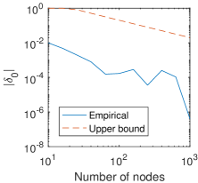
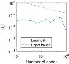
We evaluate the absolute difference between the empirical marginal probability $\widehat{\Pr}(a_{ij}=0)$ and the empirical conditional probabilities $\widehat{\Pr}(a_{ij}=0|a_{i^{\prime}j^{\prime}}=0)$ and $\widehat{\Pr}(a_{ij}=0|a_{i^{\prime}j^{\prime}}=1)$. The empirical deviation from independence is shown to be well below the upper bound in Figure 2. The bound (3) in the (Asymptotic Independence Theorem). depends only on the mean number of events, so it is somewhat loose when applied to the block Hawkes model.

5.2. Class Estimation

Figure 3. Mean adjusted Rand indices ($\pm$ standard error) for class estimation simulation experiment with varying durations. Spectral clustering with local search produces the most accurate class estimates, while the spectral initialization for variational EM does not appear to work well.

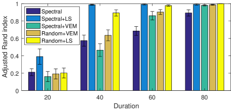
This simulation experiment is based on the synthetic network generator from Newman and Girvan (2004), where all the diagonal block pairs have the same parameters, and the off-diagonal block pairs have the same parameters, but different from the diagonal block pairs. We generate networks with $128$ nodes and $4$ classes from the block Hawkes model using Algorithm 1 with varying durations from $20$ to $80$ time units. We generate $10$ networks for each duration, with Hawkes process parameters $\alpha$ and $\beta$ being $0.6$ and $0.8$, respectively, for all block pairs. The baseline rates $\lambda^{\infty}$ are $1.8$ for diagonal block pairs and $0.6$ for off-diagonal block pairs. Classes are estimated using $5$ methods: spectral clustering, local search initialized with spectral clustering, variational EM initialized with spectral clustering, variational EM with $10$ random initializations, and local search with $10$ random initializations.

The results shown in Figure 3 demonstrate that local search initialized with spectral clustering (Spectral+LS) is the most accurate. Conversely, the spectral clustering initialization for variational EM (Spectral+VEM) results in significantly worse results. Variational EM and local search using $10$ random initializations (Random+VEM and Random+LS) take significantly longer than Spectral+LS; however, they are also less accurate, so we use Spectral+LS in the remainder of this paper.

5.3. Scalability of Local Search

(a)

(b)

Figure 4. CPU time per iteration of local search inference in seconds with varying number of nodes and events.

(a) Singular values

(b) $\alpha$: Jump sizes

(c) $\beta$: Jump decay rates

(d) $\lambda^{\infty}$: Background intensity

Figure 5. Block Hawkes model fit on Reality Mining data with 2 blocks. Nodes 1-15 belong to block 1 and the rest to block 2. LABEL:sub@fig:RealitySingularValues First 15 singular values of the adjacency matrix. LABEL:sub@fig:RealityAlpha-LABEL:sub@fig:RealityLambda Hawkes process parameter estimates.

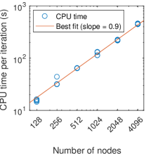
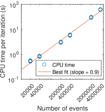
We evaluate the scalability of the proposed local search inference procedure by generating networks with varying number of nodes and events from the block Hawkes model. When varying the number of nodes, we choose a time duration of $1,200$ time units and set the Hawkes process parameters $(\alpha,\beta,\lambda^{\infty})$ to $(1.6,2,1.2)$ for diagonal block pairs and $(0.6,0.8,0.6)$ for off-diagonal block pairs. When varying the number of events, we choose a network with $128$ nodes and set the Hawkes process parameters $(\alpha,\beta,\lambda^{\infty})$ to $(0.6,0.8,1.8)$ for diagonal block pairs and $(0.6,0.8,0.6)$ for off-diagonal block pairs. We keep the number of classes fixed to be $4$ in both settings and simulate $5$ networks for each configuration.

The CPU times per iteration for both varying number of nodes and events are shown in Figure 4 along with best-fit lines for a power law relationship (beginning with $512$ nodes for the varying nodes experiment). The best-fit line has slope $0.9$ in both cases, confirming the linear time complexity both in terms of the number of nodes $N$ and the number of events $M$, which is as expected according to the computed time complexity in Section 4.1. All CPU times are recorded on a Linux workstation using $18$ Intel Xeon processor cores operating at $2.8$ GHz.

6. Real Data Experiments

6.1. MIT Reality Mining

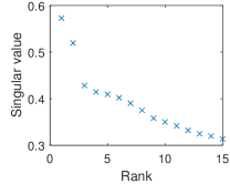
We analyze the MIT Reality Mining data (Eagle et al., 2009), using start times of phone calls as events from the caller to the recipient. Nodes in this data set correspond to students and staff at MIT. The data were collected over approximately 10 months beginning in August 2004. We remove all nodes who do not either make or receive a call at any point in the data trace, resulting in a network with 86 nodes.

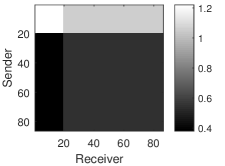
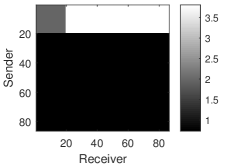
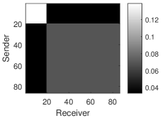
We observe a significant gap after the second largest singular value of the regularized graph Laplacian, as shown in Figure 5a so we choose $K=2$ blocks. From examining the block Hawkes model parameter estimates shown in Figure 5b-5d, block pair $(1,1)$ has both higher background intensity $\lambda^{\infty}$ and longer bursts due to high $\alpha$ and low $\beta$. Thus, not only does it appear to be a community, but phone calls within the community tend to happen in prolonged bursts. On the other hand, block pair $(2,2)$ has higher background intensity than the off-diagonal block pairs but without the large jump sizes, indicating a lack of bursty behavior compared to block pair $(1,1)$. Block pair $(1,2)$ has high values for both $\alpha$ and $\beta$, indicating large bursts of short duration. However, since block pair $(1,2)$ has a lower background intensity than $(2,2)$, the overall density of the block pair in the aggregated adjacency matrix is not necessarily higher. Indeed, block pair $(2,2)$ has a density of $0.041$, while block pair $(2,1)$ has a density of $0.034$. Thus, the continuous-time model of the network enables greater analysis of the dynamics of interactions over both short and long periods of time, and the findings may be quite different from those of static and discrete-time network representations.

6.2. Facebook Wall Posts

6.2.1. Model-Based Exploratory Analysis

(a) Singular values

(b) $\alpha$: Jump sizes

(c) $\beta$: Jump decay rates

(d) $\lambda^{\infty}$: Background intensity

Figure 6. Block Hawkes model parameter estimates on Facebook wall post data with 2 blocks. Nodes 1-1421 belong to block 1 and the rest to block 2. LABEL:sub@fig:FacebookSingularValues First 15 singular values of the adjacency matrix. LABEL:sub@fig:FacebookAlpha-LABEL:sub@fig:FacebookLambda Hawkes process parameter estimates.

We analyze the Facebook wall post data collected by Viswanath et al. (2009), which contains over $60,000$ nodes. We consider events between January 1, 2007 and January 1, 2008. We remove nodes with degree less than $10$, resulting in a network with $137,170$ events among $3,582$ nodes.

Figure 7. Hawkes process intensity function for events in block pair (1,1) of the Facebook data. Event times are denoted by black ticks along the horizontal axis.

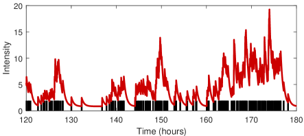
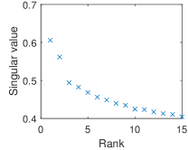
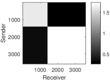
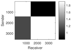
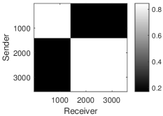
We select a model with $K=2$ blocks, as suggested by the singular values of the regularized graph Laplacian shown in Figure 6a. The parameters inferred from the BHM fit on the Facebook data are shown in Figure 6b-6d. The diagonal block pairs have larger values of background intensity $\lambda^{\infty}$, indicating that the blocks form communities. This finding could also have been yielded by static and discrete-time SBMs. The diagonal block pairs also have higher values of jump sizes $\alpha$, indicating that wall posts between members of a community are more bursty. A portion of the Hawkes process intensity function for block pair $(1,1)$ is shown in Figure 7. In addition to diurnal patterns, one can observe bursty periods of wall posts throughout the day. This finding could not have been obtained from static and discrete-time SBMs. From the values of $\alpha$ on the diagonal block pairs, we see that wall posts within block 2 are more bursty, with higher jump sizes and roughly equal jump decay rates compared to posts within block 1. By observing the values of $\alpha$ on off-diagonal block pairs, we notice that there isn’t much asymmetry, but the decay rate $\beta$ exhibits asymmetry. Specifically, events from block 1 to 2 have longer sustained bursts than events from block 2 to 1 due to the lower value of $\beta_{12}$ compared to $\beta_{21}$.

6.2.2. Comparison with Discrete-Time SBM

To compare our proposed continuous-time BHM with a discrete-time SBM (Xu and Hero III, 2014), we consider the task of predicting the time to the next event in each block pair. We believe that this is a fair comparison because both the BHM and discrete-time SBM require that pairs of nodes in the same block pair have identical edge probabilities. We split the data into two sets, with the first $8$ months of data for training and the last $4$ months for testing. During each week of the test set, we attempt to predict the time to the next event in each block pair. Afterwards, we update the model with all events during that week. This results in $16$ predictions in the test set for each block pair.

The BHM directly models event times, so we use the expected next event time for each block as the prediction. The discrete-time SBM does not directly model event times, so we multiply the expected number of time snapshots that will elapse before the next edge formation, which is geometrically distributed, by the snapshot length and then subtract half the snapshot length (to center the prediction within the snapshot) to get a prediction for the next event time. Since the prediction for the discrete-time SBM is dependent on the snapshot length, we test several different snapshot lengths.

We estimate class assignments for both models using regularized spectral clustering with $2$ classes (with no local search iterations) so that differences in class estimates between the two models do not play a role in the accuracy. We believe this is a valid comparison because spectral clustering is used as the initialization to local search in the inference procedure for both models, as discussed in Section 4.1 for the BHM and in (Xu and Hero III, 2014) for the discrete-time SBM.

We evaluate the accuracy of the predictions by computing the root mean-squared error (RMSE) between predicted event times and actual event times for the first event in each block pair during a week. Since the blocks form communities, we expect events to arrive much more frequently within blocks. Thus we separate the evaluation into within-block and between-block prediction RMSE. As shown in Figure 8, the accuracy of the discrete-time SBM is highly dependent on the snapshot length. For snapshots of 6 hours and longer, the loss in temporal resolution is the main contributor to the high RMSE. The shorter snapshots such as 1 hour and 2 hours have excellent temporal resolution for within-block prediction but are less accurate for between-block prediction. Choosing 3-hour long snapshots results in the most accurate between-block predictions. Due to the different rates of events within and between blocks, the discrete-time representation must trade off between within-block and between-block prediction accuracy when choosing the snapshot length. Using our continuous-time BHM, we avoid this complex problem of choosing the snapshot length and produce more accurate predictions (in total RMSE) than the discrete-time model for any snapshot length, as shown in Figure 8.

Figure 8. Prediction RMSE in hours for block Hawkes model and discrete-time SBMs on Facebook data.

7. Conclusion

In this paper, we introduced the block point process model (BPPM) for dynamic networks evolving in continuous time in the form of timestamped events between nodes. Our model was inspired by the well-known stochastic block model (SBM) for static networks and is a simpler version of the Hawkes IRM. We demonstrated that adjacency matrices constructed from the BPPM follow an SBM in the limit of a growing number of nodes. To the best of our knowledge, this is the first result of this type connecting point process network models with adjacency matrix network models. Additionally we proposed a principled and efficient algorithm to fit the BPPM using spectral clustering and local search that scales to large networks and apply it to analyze several real networks.

Appendix A Proof of Asymptotic Independence Theorem

We begin with a well-known lemma on the difference of powers that will be used both to upper and lower bound the deviation from independence.

Lemma A.1 (Difference of powers).

For a real number $x>1$ and integer $m\geq 1$, we have the following identity:

(7) $$m(x-1)^{m-1}\leq x^{m}-(x-1)^{m}\leq mx^{m-1}.$$

Proof.

The proof follows straightforwardly from factorizing a difference of powers. Specifically, for real numbers $x>y>0$ and integer $m\geq 1$,

(8) $$x^{m}-y^{m}=(x-y)\sum_{i=0}^{m-1}x^{m-1-i}y^{i}.$$

If $x>1$ and $y=x-1$, then (8) becomes

$$x^{m}-(x-1)^{m}=\sum_{i=0}^{m-1}x^{m-1-i}(x-1)^{i}.$$

There are $m$ terms in the summation. The largest term is $x^{m-1}$, and the smallest term is $(x-1)^{m-1}$. Thus, we can upper and lower bound the sum by $mx^{m-1}$ and $m(x-1)^{m-1}$, respectively, to arrive at (7). ∎

The next lemma will be used in the upper bound.

Lemma A.2.

For a real number $x>1$ and integer $m\geq 1$,

$$\left(\frac{n-1}{n}\right)^{m}\geq 1-\frac{m}{n}.$$

Proof.

$$\left(\frac{n-1}{n}\right)^{m}-1 =\frac{(n-1)^{m}-n^{m}}{n^{m}}$$

$$=-\frac{n^{m}-(n-1)^{m}}{n^{m}}$$

(9) $$\geq-\frac{mn^{m-1}}{n^{m}}$$

(10) $$=-\frac{m}{n},$$

where (9) follows from applying Lemma A.1. Adding $1$ to both sides of (10), we arrive at the desired result. ∎

We now prove the (Asymptotic Independence Theorem)..

Proof of (Asymptotic Independence Theorem)..

First compute the marginal probability $\Pr(a_{ij}=0)$. $a_{ij}=0$ implies that no events between nodes $i$ and $j$ occurred. To compute this probability, we first compute the conditional probability given that the number of events in block pair $b$ is $m_{b}$. To simplify notation, we drop the subscript $b$ from $m_{b}$ and $n_{b}$ in the remainder of the proof, so the conditional probability can be written as

$$\Pr(a_{ij}=0|m)=\left(\frac{n-1}{n}\right)^{m},\,m\geq 0,$$

where the equality follows by noting that, conditioned on $m$ total events in block pair $b$, the number of events between nodes $i$ and $j$ follows a binomial distribution with $m$ trials and success probability $1/n$. The $1/n$ success probability is due to step 8 of the generative process of the BPPM, which involves selecting node pairs randomly to receive an event. By the Law of Total Probability, the marginal probability is

$$\Pr(a_{ij}=0) =\sum_{m=0}^{\infty}p(m)\Pr(a_{ij}=0|m)$$

(11) $$=\sum_{m=0}^{\infty}p(m)\left(\frac{n-1}{n}\right)^{m},$$

where the probability mass function $p(m)$ denotes the probability that $m$ events in block pair $b$ occurred.

Next consider the joint probability $\Pr(a_{ij}=0,a_{i^{\prime}j^{\prime}}=0)$. As before, condition on the number of events $m$. The conditional joint probability is

$$\Pr(a_{ij}=0,a_{i^{\prime}j^{\prime}}=0|m)=\left(\frac{n-2}{n}\right)^{m},\;m\geq 0,$$

because the number of events for each node pair in block pair $b$ follow a multinomial distribution with $m$ trials and all event probabilities equal to $1/n$. By the Law of Total Probability,

(12) $$\Pr(a_{ij}=0,a_{i^{\prime}j^{\prime}}=0)=\sum_{m=0}^{\infty}p(m)\left(\frac{n-2}{n}\right)^{m}.$$

We first lower bound $\delta_{0}$ by noting that

$$\delta_{0} =\Pr(a_{ij}=0|a_{i^{\prime}j^{\prime}}=0)-\Pr(a_{ij}=0)$$

$$\geq\Pr(a_{ij}=0,a_{i^{\prime}j^{\prime}}=0)-\Pr(a_{ij}=0)$$

(13) $$=\sum_{m=0}^{\infty}p(m)\left[\left(\frac{n-2}{n}\right)^{m}-\left(\frac{n-1}{n}\right)^{m}\right]$$

$$=-\sum_{m=0}^{\infty}p(m)\frac{(n-1)^{m}-(n-2)^{m}}{n^{m}}$$

(14) $$\geq-\sum_{m=0}^{\infty}p(m)\frac{m(n-1)^{m-1}}{n^{m}}$$

$$=-\frac{1}{n}\sum_{m=0}^{\infty}mp(m)\left(\frac{n-1}{n}\right)^{m-1}$$

(15) $$\geq-\frac{1}{n}\sum_{m=0}^{\infty}mp(m)$$

(16) $$=-\frac{\mu}{n},$$

where (13) follows from (11) and (12), (14) follows from Lemma A.1, and (15) follows by observing that $\big{(}\frac{n-1}{n}\big{)}^{m-1}\leq 1$.

We now upper bound $\delta_{0}$ by noting that

$$\delta_{0} =\Pr(a_{ij}=0|a_{i^{\prime}j^{\prime}}=0)-\Pr(a_{ij}=0)$$

$$\leq 1-\Pr(a_{ij}=0)$$

$$=1-\sum_{m=0}^{\infty}p(m)\left(\frac{n-1}{n}\right)^{m}$$

(17) $$\leq 1-\sum_{m=0}^{\infty}p(m)\left(1-\frac{m}{n}\right)$$

$$=1-\sum_{m=0}^{\infty}p(m)+\frac{1}{n}\sum_{m=0}^{\infty}mp(m)$$

$$=1-1+\frac{\mu}{n}$$

(18) $$=\frac{\mu}{n},$$

where (17) follows from Lemma A.2.

Next we lower bound $\delta_{1}$ by noting that

$$\delta_{1} =\Pr(a_{ij}=0|a_{i^{\prime}j^{\prime}}=1)-\Pr(a_{ij}=0)$$

$$=\frac{\Pr(a_{ij}=0,a_{i^{\prime}j^{\prime}}=1)-\Pr(a_{ij}=0)\Pr(a_{i^{\prime}j^{\prime}}=1)}{\Pr(a_{i^{\prime}j^{\prime}}=1)}$$

$$\geq\Pr(a_{ij}=0,a_{i^{\prime}j^{\prime}}=1)-\Pr(a_{ij}=0)\Pr(a_{i^{\prime}j^{\prime}}=1)$$

$$=\Pr(a_{ij}=0)-\Pr(a_{ij}=0,a_{i^{\prime}j^{\prime}}=0)$$

$$\qquad-\Pr(a_{ij}=0)[1-\Pr(a_{i^{\prime}j^{\prime}}=0)]$$

$$=-[\Pr(a_{ij}=0,a_{i^{\prime}j^{\prime}}=0)-\Pr(a_{ij}=0)\Pr(a_{i^{\prime}j^{\prime}}=0)]$$

$$=-\Pr(a_{i^{\prime}j^{\prime}}=0)[\Pr(a_{ij}=0|a_{i^{\prime}j^{\prime}}=0)-\Pr(a_{ij}=0)]$$

$$=-\Pr(a_{i^{\prime}j^{\prime}}=0)\delta_{0}$$

$$\geq-\delta_{0}$$

(19) $$\geq-\frac{\mu}{n},$$

where (19) follows from (18).

Finally we upper bound $\delta_{1}$ using the same approach as for $\delta_{0}$:

$$\delta_{1} =\Pr(a_{ij}=0|a_{i^{\prime}j^{\prime}}=1)-\Pr(a_{ij}=0)$$

$$\leq 1-\Pr(a_{ij}=0)$$

(20) $$\leq\frac{\mu}{n},$$

where the final inequality is obtained from (18).

Combining (16), (18), (19), and (20), and noting that the maximum deviation between two probabilities is $1$, we arrive at the desired result $|\delta_{0}|,|\delta_{1}|\leq\min\{1,\mu/n\}$, which completes the proof. ∎

Appendix B Variational Inference Details

We begin by deriving the complete-data log-likelihood for the block point process model.

$$\log \Pr(E,Z|\theta,\boldsymbol{\mathbf{\pi}})$$

$$=\log\Pr(Z|\boldsymbol{\mathbf{\pi}})+\log\Pr(\boldsymbol{\mathbf{u}},\boldsymbol{\mathbf{v}},\boldsymbol{\mathbf{t}}|Z,\theta)$$

(21) $$=\log\Pr(Z|\boldsymbol{\mathbf{\pi}})+\log\Pr(\boldsymbol{\mathbf{u}},\boldsymbol{\mathbf{v}}|Z)+\log\Pr(\boldsymbol{\mathbf{t}}|\boldsymbol{\mathbf{u}},\boldsymbol{\mathbf{v}},Z,\theta)$$

The first term in (21) represents the prior class probability and is given by

$$\log\Pr(Z|\boldsymbol{\mathbf{\pi}})=\log\left(\prod_{i=1}^{N}\prod_{q=1}^{K}\pi_{iq}^{z_{iq}}\right)=\sum_{i=1}^{N}\sum_{q=1}^{K}z_{iq}\log(\pi_{iq}).$$

The second term in (21) represents the uniform distribution of events to nodes inside a block pair and is given by

$$\log\Pr(\boldsymbol{\mathbf{u}},\boldsymbol{\mathbf{v}}|Z) =\log\left[\prod_{q=1}^{K}\prod_{l=1}^{K}\left(\frac{1}{n_{ql}}\right)^{m_{ql}}\right]$$

$$=-\sum_{q=1}^{K}\sum_{l=1}^{K}m_{ql}\log(n_{ql})$$

$$=-\sum_{q=1}^{K}\sum_{l=1}^{K}\boldsymbol{\mathbf{z}}_{:q}^{T}W\boldsymbol{\mathbf{z}}_{:l}\log(\boldsymbol{\mathbf{z}}_{:q}^{T}\boldsymbol{\mathbf{z}}_{:l}),$$

where $m_{ql}$ and $n_{ql}$ are defined in the same manner as $m_{b}$ and $n_{b}$ in Section 4.1. The last equality represents these two terms as a function of $Z$, where $\boldsymbol{\mathbf{z}}_{:q}$ denotes the $q$th column of $\boldsymbol{\mathbf{z}}$, and a weighted adjacency matrix $W$ where the weight $w_{ij}$ corresponds to the total number of events from node $i$ to node $j$. The third term in (21) depends on the choice of point process; for the block Hawkes model, it is given by

$$\log \Pr(\boldsymbol{\mathbf{t}}|\boldsymbol{\mathbf{u}},\boldsymbol{\mathbf{v}},Z,\theta)=\sum_{q=1}^{K}\sum_{l=1}^{K}\Biggl{(}\sum_{s=1}^{M}\Biggl{\{}z_{u_{s}q}z_{v_{s}l}\frac{\alpha_{ql}}{\beta_{ql}}\left[e^{-\beta_{ql}(t_{M}-t_{s})}-1\right]$$

$$+\log\left[\lambda_{ql}^{\infty}+\sum_{r=1}^{s-1}z_{u_{r}q}z_{v_{r}l}\alpha_{ql}e^{-\beta_{ql}(t_{s}-t_{r})}\right]\Biggr{\}}-t_{M}\lambda_{ql}^{\infty}\Biggr{)},$$

where $u_{s}$ and $v_{s}$ denote the sender and receiver nodes for event $s$. The complete-data log-likelihood (21) is intractable since changing the class membership of one node might affect the class memberships of other nodes, so all possibilities of $Z$ need to be considered.

We derive a mean-field variational inference procedure in which we approximate the posterior with the fully factorizable variational distribution given by (6). We now try to find the best distribution from the family of multinomial distributions that can get us closest in KL divergence to the posterior. But calculating KL divergence requires calculating the intractable posterior, so we instead maximize the evidence lower bound (ELBO), which is equivalent to minimizing KL divergence (Blei et al., 2017). The ELBO is given by

$$\text{ELBO}(R_{E})=\operatorname{\mathbb{E}}\left[\log\Pr(E,Z|\theta,\boldsymbol{\mathbf{\pi}})\right]-\operatorname{\mathbb{E}}\left[\log R_{E}(Z)\right].$$

Now expand and calculate expectation of individual terms in the complete-data log-likelihood (21). The expectation of the log of the summations in the second and third terms in (21) can be bounded using Jensen’s inequality:

$$\operatorname{\mathbb{E}}[f(x)]\geq f(\operatorname{\mathbb{E}}(x)).$$

After bounding the log sums using Jensen’s inequality and calculating the expectations with respect to $R_{E}$, we arrive at the simplified expression for the ELBO:

$$\mathcal{E} (R_{E})=\sum_{i=1}^{N}\sum_{q=1}^{K}\tau_{iq}\log(\pi_{iq})-\sum_{q=1}^{K}\sum_{l=1}^{K}\boldsymbol{\mathbf{\tau}}_{:q}^{T}W\boldsymbol{\mathbf{\tau}}_{:l}\log(\boldsymbol{\mathbf{\tau}}_{:q}^{T}\boldsymbol{\mathbf{\tau}}_{:l})$$

$$+\sum_{q=1}^{K}\sum_{l=1}^{K}\Biggl{(}\sum_{s=1}^{M}\Biggl{\{}\tau_{u_{s}q}\tau_{v_{s}l}\frac{\alpha_{ql}}{\beta_{ql}}\left[e^{-\beta_{ql}(t_{M}-t_{s})}-1\right]+\log\Biggl{[}\lambda_{ql}^{\infty}$$

(22) $$+\sum_{r=1}^{s-1}\tau_{u_{r}q}\tau_{v_{r}l}\alpha_{ql}e^{-\beta_{ql}(t_{s}-t_{r})}\Biggr{]}\Biggr{\}}-t_{M}\lambda_{ql}^{\infty}\Biggr{)}+\sum_{i=1}^{N}\sum_{q=1}^{K}\tau_{iq}\log(\tau_{iq})$$

where $\boldsymbol{\mathbf{\tau}}_{:q}$ denotes the vector of variational parameters for class $q$ over all $N$ nodes. The variational expectation-maximization (VEM) algorithm alternates between a variational E step, in which we use coordinate ascent to optimize the ELBO (22) over the variational parameters $\boldsymbol{\mathbf{\tau}}_{i}$ for each node $i$, and an M step, in which we optimize the ELBO over the Hawkes process parameters $\big{(}\alpha_{ql},\beta_{ql},\lambda_{ql}^{\infty}\big{)}$ for all block pairs $(q,l)\in\{1,\ldots,K\}^{2}$.