Testing Modified Gravity Theories via Wide Binaries and GAIA

Abstract

The standard $\Lambda$CDM model based on General Relativity (GR) including cold dark matter (CDM) is very successful at fitting cosmological observations, but recent non-detections of candidate dark matter (DM) particles mean that various modified-gravity theories remain of significant interest. The latter generally involve modifications to GR below a critical acceleration scale $\sim 10^{-10}\,{\rm m\,s^{-2}}$. Wide-binary (WB) star systems with separations $\ga 5\,{\rm kAU}$ provide an interesting test for modified gravity, due to being in or near the low-acceleration regime and presumably containing negligible DM. Here, we explore the prospects for new observations pending from the GAIA spacecraft to provide tests of GR against MOND or TeVes-like theories in a regime only partially explored to date. In particular, we find that a histogram of (3D) binary relative velocities, relative to equilibrium circular velocity predicted from the (2D) projected separation predicts a rather sharp feature in this distribution for standard gravity, with an 80th (90th) percentile value close to 1.025 (1.14) with rather weak dependence on the eccentricity distribution. However, MOND/TeVeS theories produce a shifted distribution, with a significant increase in these upper percentiles. In MOND-like theories without an external field effect, there are large shifts of order unity. With the external field effect included, the shifts are considerably reduced to $\sim 0.04-0.08$, but are still potentially detectable statistically given reasonably large samples and good control of contaminants. In principle, followup of GAIA-selected wide binaries with ground-based radial velocities accurate to $\la 0.03{\rm\,km\,s^{-1}}$ should be able to produce an interesting new constraint on modified-gravity theories.

1 Introduction

Einstein’s theory of General Relativity (GR) provides the best known description of gravity on all scales. However, much cosmological data (Ade et al., 2016) requires an additional cold, non-baryonic & non-visible dark matter (DM) component to match many observations, in addition to dark energy such as a cosmological constant. At the present time there is no decisive direct detection of DM (e.g. Akerib et al. (2017)); this leaves an open window for possible modified-gravity theories which may possibly account for these effects without the inclusion of exotic DM.

The MOdified Newtonian Dynamics (MOND) is a notable theory that attempts to explain weak-field/non-relativistic gravitational effects without DM. This theory was first proposed by Milgrom (1983) to explain the flat rotation curves observed in most spiral galaxies without requiring DM. The original MOND formulation was non-relativistic and really a fitting function rather than a realistic theory; it has later been incorporated into relativistic theories following from the well-known Tensor-Vector-Scalar (TeVeS) theory proposed by Bekenstein (2004).

So far, no modified-gravity theory (without DM) has been close to successful in fitting the cosmic microwave background (CMB) observations from WMAP and Planck (Ade et al., 2016), hence the $\Lambda$CDM model remains the standard model. But, there is a large model space for modified gravity which remains only partially explored, and currently there does not exist any “No-Go theorem” demonstrating that no plausible modified-gravity theory could match the CMB and other cosmological data in the future. In the absence of either a convincing direct detection of dark matter, or a future general No-Go theorem, or new observations excluding modified gravity at the relevant very low accelerations, the situation is likely to remain unsettled; new tests which can discriminate between DM and modified-gravity are highly desirable.

In this work we consider the prospects for a test of gravity in the low-acceleration regime via wide binary (WB) stellar systems; previous work in this area has been done by Hernandez et al. (2011),Hernandez et al. (2012), Hernandez et al. (2014) and Matvienko & Orlov (2015); these gave hints of deviations in the direction expected from MOND-like gravity, though due to the limited precision of current data, these hints are not yet decisive.

Here we extend on the work of Hernandez and co-workers above, but focusing on the much improved precision which will be possible with GAIA data; we also explore the external field effect of MOND and add new statistical tests.

Similar to Hernandez et al. (2011), Hernandez et al. (2012), Hernandez et al. (2014) and Matvienko & Orlov (2015), we consider WBs with separations $r\ga 3\,{\rm kAU}$, for which recent samples have been selected by e.g. Scarpa et al. (2017); Coronado & Chaname (2015); Andrews et al. (2017).

For a typical stellar WB with a separation $r\sim 7000\,{\rm AU}$, and masses $M\sim 1\,M_{\odot}$, the acceleration is $a\sim 10^{-10}\,{\rm m\,s^{-2}}$ which is comparable to the critical acceleration constant $a_{0}$ in MOND-like theories, and also similar to the local gravitational acceleration due to our Milky Way galaxy.

The formation mechanism of WBs is not well known, but may well result from captures during evaporation of star-forming clusters; the key point for the present purposes is that WBs are not expected to contain any significant amount of DM, so their distribution in orbital parameters should follow GR/Newtonian predictions apart from perturbations from Galactic tides, giant molecular clouds and passing stellar fly-bys. These perturbations are significant, but disrupted binaries should separate out to many-parsec separations on a timescale $\sim 10$ Myr which is much shorter than the age of the Galaxy; thus there should be a reasonably clear distinction between currently-bound and disrupted wide binaries.

Previous work of Yoo et al. (2003) & Quinn et al. (2009) used a WB sample selected by Chaname & Gould (2004), and examined the distribution of angular separations. The observed distribution is consistent with a power-law; tidal disruption by an external perturbing source such as Galactic & disk tides, giant molecular clouds or massive compact halo objects (MACHOs) would preferentially disrupt the widest binaries, inducing a break in this power-law at large separations. An upper limit on such a break can bound the abundance of massive perturbers, placing upper limits on the abundance of dark-halo MACHOs of mass $\ga 100\,M_{\odot}$.
The main observational challenge with WBs is that their orbital periods are extremely long (and accelerations and velocity differences very small), so realistic observations provide only a instantaneous snapshot of position and velocity differences, and individual orbit solutions are not possible. However, statistical distributions of velocity differences for a large sample of wide binary systems can still provide an interesting constraint, as we explore below.

In this paper we numerically compute the observables for samples of simulated WB systems with various assumed gravity models, including GR/Newton and several MoND/TeVes models. We predict their velocity ratio vs projected separation distribution that would be derived from on-going observations with GAIA, and future observations with high-precision ground-based radial velocity measurements. The plan of the paper is as follows: in Section 2 we provide an overview of the issues, define our notation and recap some standard results for Newtonian orbits. In Section 3 we review some selected theories of modified gravity as they pertain to the next sections. In Section 4 we produce simulations of WB orbits for various gravity theories, and we produce forecasts of observables. In Section 5 we discuss some additional observational issues, and in Section 6 we summarise the conclusions.

2 Wide Binaries and GAIA

Here we define “wide binaries” as those with orbital accelerations comparable to the MOND acceleration parameter $a_{0}$, commonly defined as $a_{0}\simeq 1.2\times 10^{-10}\,{\rm m\,s^{-2}}$, or separations above $\sim 7\,{\rm kAU}$ for Solar-mass binaries. Wide binaries have received relatively little attention in the past for several reasons: their orbital periods ($\sim$ Myr) are so long that no deviations from linear motion are detectable on a realistic timescale: thus full orbit solutions are impossible, and any reasonable observing programme gives us only a snapshot of some subset of the six phase-space parameters (three relative positions and three relative velocities). Also, their relative velocities of order $\sim 0.3{\rm\,km\,s^{-1}}$ translate to expected proper motion differences of order 0.6 milliarcsec (mas) per year at an example distance of 100 pc, which is near the limits of achievable $1\sigma$ measurement precision in the pre-GAIA era. Finally, uncertainties in available parallax distances translate to significant stellar mass uncertainties which further blurs any possible constraints. Thus, wide binaries can be selected fairly robustly with pre-GAIA data as from Hipparcos (Lepine & Bongiorno, 2007), the SlowPOKES search from SDSS (Dhital et al., 2010), and Tokovinin & Kiyaeva (2016), using proper motions to reject most chance-projection candidates or unbound fly-by pairs; but the relative velocity precision is currently not sufficient to use the resulting binaries for dynamical tests.

Also, there is a notable gap in previous wide binary catalogues: Hipparcos parallaxes are generally limited to magnitude $V\la 10$, while SDSS imaging saturates for stars at $V\la 14$, which leaves the magnitude range $10<V<14$ rather less explored for wide binaries. This magnitude range includes millions of stars, with potentially $\sim 0.5$ million closer than $\approx 200\,{\rm pc}$, and many thousand wide binaries (see Section 5.1) which are bright enough to follow-up with high-quality ground-based spectroscopy.

The GAIA spacecraft (Prusti et al., 2016) will dramatically transform this situation: firstly, its proper motion precision after the baseline 5-year mission is predicted to be around 15 microarcsec per year ($\,\mu{\rm as}\,{\rm yr}^{-1}$) at magnitude $G\simeq 15$ (Prusti et al., 2016); multiplying by $\sqrt{2}$ for the differential motion between two stars translates to a very small transverse velocity uncertainty of $\sim 0.01{\rm\,km\,s^{-1}}$ at our example $100\,{\rm pc}$ distance, which is much smaller than expected binary orbital velocities at separations $\sim 10\,{\rm kAU}$. Secondly, GAIA will provide high-precision parallax distances (better than 1% for the above parameters) and hence precise luminosities, while metallicities can readily be obtained either from the GAIA spectra or from the ground for these bright stars. Using a mass-luminosity-metallicity relation, for main-sequence stars we can then infer masses for both components of wide binaries; uncertainties such as age may limit this to perhaps 5 percent mass precision, but this is essentially good enough for the following purposes.

The GAIA distance precision (e.g. 0.3 percent at $100\,{\rm pc}$) is usually not quite good enough to resolve the line-of-sight separation of a typical wide binary at $r\sim 3-20\,{\rm kAU}$ (though for very nearby and wide systems at $\sim 20\,{\rm pc}$, resolving the line-of-sight separation should be possible); however it is good enough to weed out the vast majority of chance-projection interlopers: observed star pairs with small projected separation $\la 20\,{\rm kAU}$, 3-D velocity difference $<1{\rm\,km\,s^{-1}}$ and line-of-sight separation $\la 0.5\,{\rm pc}$ are highly likely to be either true bound binaries, or unbound but physically associated pairs with a common origin, since unrelated chance-flyby pairs with such small differences should be very rare (see later).

For radial velocities, the GAIA precision is not good enough, but modern high-stability ground-based spectrographs can reach absolute accuracy $\sim 0.02{\rm\,km\,s^{-1}}$ (probably limited by systematics, see Section 5 later).

Thus, with GAIA plus high-accuracy radial velocity followup, we can get fairly precise measurements of 5 of the 6 phase-space differences for wide binaries (subject to perspective-rotation effects, discussed later), with the relative-velocity precision of order 10 percent; this turns out to be enough to get potentially interesting tests of gravity in the low-acceleration regime where any modified-gravity effects should start to become significant.

2.1 External perturbations on wide binaries

Wide binaries are weakly bound and thus are significantly sensitive to perturbations from either fly-by encounters with passing stars, from giant molecular clouds, or from Galactic tidal effects. Tidal effects are expected to disrupt binaries beyond the Jacobi radius around $1.7\,{\rm pc}$ or $350\,{\rm kAU}$ for a typical binary; this is over an order of magnitude larger than the separations considered below, but tidal effects may be non-negligible at smaller scales. A numerical simulation of these effects has been made by Jiang & Tremaine (2010) (JT10), with the following main conclusions.

The survival probability for a wide binary over 10 Gyr is a declining function of semi-major axis, with estimated 50 percent survival probability occurring at a separation of around $30\,{\rm kAU}$. Binaries which become unbound do not always separate completely, but can remain within 10 parsec separation for many Gyr after unbinding. The histogram of separations for binaries evolved over 10 Gyr shows a minimum at $\sim 3\,r_{J}$ or $5\,{\rm pc}$, then a secondary maximum at $\sim 10\,{\rm pc}$. Also, Figure 3 of JT10 shows that the distribution of projected separations at $r\la 10\,{\rm kAU}$ largely follows the initial distribution, which is promising for the tests below. This suggests that external perturbations may significantly randomise the eccentricity distribution of binaries at $\sim 10\,{\rm kAU}$, but we see below that our results are relatively insensitive to this poorly-known eccentricity distribution. The RMS (line of sight) velocity difference of the simulated binaries in JT10 closely follows the expected Keplerian falloff $\propto r_{p}^{-0.5}$ out to projected separations $\sim 0.3\,r_{J}$ or $100\,{\rm kAU}$ (as shown in Figure 7 of JT10).

Since our main focus below is on binaries of present-day projected separation between $3$ to $20\,{\rm kAU}$, we expect that external perturbations are not a major source of uncertainty in this range, though further numerical work would be desirable to quantify this more precisely.

2.2 Distribution of velocity differences

We start here considering an idealised case assuming a wide binary where both masses and all six relative separation and velocity components are reasonably well measured; then consider practical deviations from this later.

If we have a candidate binary of estimated masses $M_{1},M_{2}$ at (3D) separation $r$, we define a convenient dimensionless parameter $u_{3D}\equiv v_{\rm 3D}/v_{C}(r)$ where $v_{\rm 3D}$ is the magnitude of the instantaneous (3D) velocity difference, and $v_{C}(r)$ is the velocity for a circular Newtonian orbit at the current separation $r$ (note, not the unknown semi-major-axis $a$). Clearly $v_{C}(r)=\left[G(M_{1}+M_{2})/r\right]^{0.5}$.

In terms of the semi-major axis $a$ and eccentricity $e$, we then have

$$u_{3D}=\sqrt{2-r/a}\ ,$$ (1)

with the well-known result that $u_{3D}<\sqrt{2}$ for any bound orbit. In general for any bound binary with eccentricity $e<1$, we have $1-e\leq u_{3D}^{2}\leq 1+e$. Considering the probability distribution for $u_{3D}$ for a large sample of binaries observed at a random time (i.e. now), it turns out that values of $u\ga 1.2$ are rather uncommon, since low-$e$ binaries never exceed this value, while high-$e$ binaries do so, but only for a rather small fraction of time around orbit pericenter.

For an assumed eccentricity $e$ and an arbitrary threshold value, $u_{th}$, we can readily compute the fraction of time over which the instantaneous value of $u_{3D}$ exceeds a chosen threshold $u_{th}$, as follows. In terms of true anomaly (angle from pericenter) $\theta$, we have

$$u_{3D}^{2}=2-\frac{1-e^{2}}{1+e\cos\theta}$$

Rearranging for a chosen threshold value $u=u_{th}$, we find in the case $1-e<u_{th}^{2}<1+e$ then $u$ crosses $u_{th}$ twice per orbit, at $\theta$ given by

$$\cos\theta_{th}=\frac{1+e^{2}-u_{th}^{2}}{e(u_{th}^{2}-2)}\ .$$ (2)

The corresponding eccentric anomaly $E_{th}$ is

$$E_{th}=2\arctan\left(\sqrt{\frac{1-e}{1+e}}\tan(\theta_{th}/2)\right)$$ (3)

and the mean anomaly $M_{th}$ follows from Kepler’s equation

$$M_{th}=E_{th}-e\sin E_{th}\ ,$$ (4)

where $\theta_{th},E_{th}$ and $M_{th}$ each have two solutions of opposite sign. Since mean anomaly is just time rescaled to $2\pi$ per orbit, the fraction of time for which a Kepler orbit of given eccentricity $e$ exceeds a chosen threshold value $u_{th}$ is then simply

$$P(u>u_{th}\,|\,e)=M_{th}/\pi\ ,$$ (5)

which is given by successive substitutions into Eqs. (2 – 5).

(Note in the special case $u_{th}=1$, this occurs on the minor axis where $\cos\theta_{th}=-e$, and it is easily seen that $P(u>1)=1/2-e/\pi$, which decreases linearly from 1/2 at small $e$ to 0.182 as $e\rightarrow 1$).

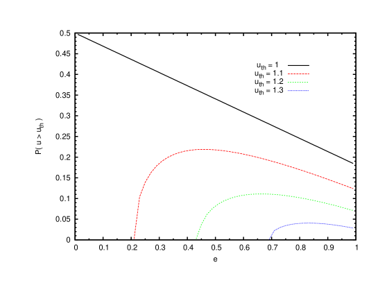
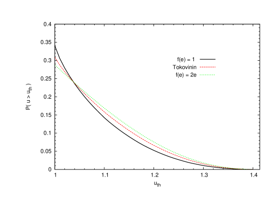
Figure 1: Fraction of time for which a Kepler orbit exceeds a selected velocity ratio $u_{th}$ as a function of eccentricity $e$, for values of $u_{th}=1.0,$ 1.1, 1.2, 1.3 (top to bottom).

Figure 2: Fraction of all orbits (at a random time) which exceed a given velocity ratio $u_{th}$ on the abscissa, for several chosen distribution functions of eccentricity: solid curve for $f(e)=1$, dashed curve for Tokovinin distribution, and dotted curve for $f(e)=2\,e$.

The resulting probability is shown as a function of $e$ for several example thresholds $u_{th}=1.0,1.1,1.2,1.3$ in Figure 2. The result (for the case $u_{th}>1$) is that this probability is zero for $e<u_{th}^{2}-1$, then rises rather quickly to a maximum then slowly declines towards $e=1$. The maximum probability is 0.219, 0.111 and 0.041 respectively for $u_{th}=1.1,1.2,1.3$, therefore a notable feature here is that the fraction of bound binaries with $u>1.2$ (at a random observing time) cannot exceed 11.1 percent (the case for a distribution of $e$ sharply peaked around $e\approx 0.67$), while for a realistic spread of $e$ values, the fraction must be smaller than 11.1 percent.

To get the predicted distribution of $u$ for a large sample of binaries with an assumed distribution function of eccentricities $f(e)$, we can simply integrate the above function in Eq. (5) weighted by the assumed $f(e)$. The result of this is shown in Figure 2 for three selected distributions of $e$: firstly a uniform distribution $f(e)=1$, secondly a Tokovinin distribution $f(e)=0.4+1.2e$, and thirdly a “dynamical” distribution $f(e)=2\,e$. Due to the shape of $P(u>u_{th}|e)$ above, the result turns out to be only weakly sensitive to the eccentricity distribution, and there is always a steeply-falling tail at $u\ga 1.2$. Taking the Tokovinin distribution as an intermediate case, we find that (at a random time) 30.9 percent of binaries have $u_{3D}>1$, while 15.8 percent have $u>1.1$, 6.6 percent have $u>1.2$, and only 1.5 percent have $u>1.3$. The 80th and 90th percentiles are at $u=1.065$ and $1.158$ respectively. These percentages change only marginally for the flat or dynamical eccentricity distributions.

Therefore, in an idealised case of a moderately large but plausible sample of candidate wide binaries (e.g. few hundred to few thousand) all with $u_{3D}$ measurements, standard gravity predicts that a histogram of $u_{3D}$ should exhibit a smoothly rising distribution at $0<u<1$ followed by a rather steep decline between $u\sim 1.1$ and $1.3$; and the location of this “ramp” feature around the 80th to 90th percentiles is only weakly sensitive to the poorly known distribution of $e$. The inevitable contamination from unbound pairs is expected to show a relatively flat or moderately rising distribution of $u_{3D}$ at $u_{3D}>\sqrt{2}$; we may need to model this contamination and subtract an estimated number of contaminants scattered to $u_{3D}<\sqrt{2}$, but as long as unbound chance pairs do not dominate the sample, the 80th/90th percentiles for bound binaries should be statistically correctable for contamination.

2.3 Projection to 2D separations

The above was assuming an idealised case where all six components of separation and relative velocities are available: but in practice, $u_{3D}$ is not directly measurable due to the uncertain line-of-sight component of the separation vector; however, the 3D relative velocity and the 2D projected separation are accurately measured, so we can make do with $u_{2D}$, defined as the ratio of 3D relative velocity to the circular velocity calculated at the observed 2D projected separation. This is then given by

$$u_{2D}=u_{3D}\sqrt{\sin\beta}$$

where $\beta$ is the unknown angle between the current binary separation vector and the line-of-sight; for random aligments, the median value of $\sin\beta$ is $\sqrt{3}/2$, so the median of the $\sqrt{\sin\beta}$ factor is 0.931, only slightly less than 1. Therefore, the effect of convolution with random aligment angles is to shift the distribution function of $u_{2D}$ to somewhat smaller values compared to $u_{3D}$, but it does not erase the steep decline in the distribution. The quantitative effects of this projection to 2D projected separations are included below in Section 4, using numerical simulations.

We note that a uniform distribution in $\cos\beta$ gives the distribution of projected separation $r_{p}$ at a given 3D separation $r$. The inverse question, of the posterior probability distribution of $r$ at a known $r_{p}$, is not quite the same question, and in this case the result depends on the intrinsic frequency distribution of $r$; however, assuming a reasonably smooth distribution in $\log r$ this distinction is relatively unimportant.

2.4 Perspective effects

It was shown by Shaya & Olling (2011) (hereafter SO11) that there are several effects implying that wide binary velocity differences are not simply given by subtracting the measured proper motions and radial velocities; we refer to these collectively as perspective effects, since they are mostly related to the system barycentre motion (relative to the Sun) causing a time-dependent perspective on the system from our location.

SO11 gave a derivation of these effects to first order in binary separation angle $\alpha=(\Delta\ell,\Delta b)$ with the key results given in their Eqs. 29, 30. We find that is somewhat more intuitive to re-arrange SO11 Eq. 29 into the form

$$\Delta{\mn@boldsymbol{\mu}}=-\mn@boldsymbol{\mu}\,\frac{\Delta d}{d}+\Delta\ell\sin b\begin{pmatrix}\mu_{b}\\ -\mu_{\ell}\end{pmatrix}-\frac{v_{r}}{d}\begin{pmatrix}\Delta\ell\cos b\\ \Delta b\end{pmatrix}\ .$$ (6)

which gives the apparent proper motion difference for a hypothetical “static” binary; where $(\ell,b)$ are Galactic coordinates, $\mn@boldsymbol{\mu}=(\mu_{\ell},\mu_{b})$ is the proper motion 2-vector and $\mu_{\ell}\equiv(d\ell/dt)\cos b$ includes the $\cos b$ factor; $d$ is distance and $v_{r}$ is radial velocity of the barycentre, and $\Delta$’s denote differences between the two components of the binary.

These three terms each have an intuitive geometrical explanation: the first term on the RHS corresponds to the closer component appearing to overtake the more distant component in the direction parallel to the proper motion.

The second term is now seen as a pure coordinate-curvature effect: if we consider tangent-plane coordinates at the barycentre, constant-$b$ lines appear as conic sections, which are locally equivalent to circular arcs with a radius of curvature of $\cot b$. The component of binary separation in the $\ell$ direction is $\approx\Delta\ell\,\cos b$, hence the constant-$b$ curves through the primary and secondary have a relative rotation angle in the tangent plane by $\approx\Delta\ell\cos b/\cot b=\Delta\ell\sin b$ . The second term above therefore is equivalent to the difference between the barycentre proper motion vector, and a copy of itself rotated by this (small) angle.

The third term is simply an apparent contraction/expansion of the binary angular separation at a fractional rate of $-v_{r}/d$.

Also, Eq. 30 of SO11 may be written as

$$\Delta v_{r}=\begin{pmatrix}d\mu_{l}\\ d\mu_{b}\end{pmatrix}\cdot\begin{pmatrix}\Delta\ell\cos b\\ \Delta b\end{pmatrix}$$ (7)

which is the scalar product of the tangential velocity vector with the binary separation angle. This may be combined with $d\times$ the first term in Eq. 6, in which case the resultant 3D velocity corresponds to a rotation of the 3D binary separation vector at an angular speed $\mu$ around the line perpendicular to both the line of sight and the proper motion vector, i.e. a “perspective rotation”. This perspective rotation effect is important; the effect on $\Delta v_{r}$ in Eq. 7 is calculable given the known angular offset and proper motion, but the effect on transverse velocity in Eq. 6 is proportional to $\Delta d/d$, and $\Delta d$ is generally not measurable to useful precision even with GAIA data.

The above analysis based on SO11 is valid up to terms first-order in binary separation angle. These are definitely important, since for typical values of system barycentre motion $v_{sys}\sim 50{\rm\,km\,s^{-1}}$, angular separation $\alpha\sim 20\,{\rm kAU}$ / 100 pc $\sim 0.001\,\text{rad}$, and $\Delta d/d\sim 0.001$, terms of order $v_{sys}\alpha$ are $\sim 0.05{\rm\,km\,s^{-1}}$, of order 20 percent of the binary relative velocity $\sim 0.25{\rm\,km\,s^{-1}}$; this is modest but not negligible. However, this may be constrained e.g. by rejecting a tail of binaries with higher transverse velocities; it is also helpful that the effect (in velocity units) decreases with distance for fixed binary separation.

We note that terms of order $v_{sys}\alpha^{2}$ are generally negligible except for very nearby or extremely wide binaries (few-degree separations), so the first-order treatment given by Shaya & Olling (2011) is adequate except for very nearby or extremely wide binaries.

3 Modified gravity models

In this section we review some of the various modified-gravity scenarios studied in the literature as possible alternatives to dark matter; these are then applied to simulated orbits of wide binaries in the following Section 4

3.1 MOND

The phenomenology known as Modified Newtonian Dynamics (MOND) was originally introduced in the 1980’s by Milgrom (1983), and has led to many variants and refinements later (see (Famaey & McGaugh, 2012) for a comprehensive review). The original motivation for MOND was to modify Newton’s second law $F_{N}=ma$ in order to attempt to account for observed effects such as flat rotation curves of spiral galaxies without the need for DM. The modification to Newton’s second law is made by introducing a critical acceleration constant, $a_{0}$, and a free function $\mu(x)$, where the dimensionless $x\equiv a/a_{0}$ is the ratio of acceleration to $a_{0}$, such that

$$a_{N}=\mu\bigg{(}\frac{a_{M}}{a_{0}}\bigg{)}a_{M}.$$ (8)

where $a_{N}$ is the GR/Newtonian acceleration, $a_{0}\approx 1.2\times 10^{-10}\,{\rm m\,s^{-2}}$ is the acceleration constant and $a_{M}$ is the acceleration predicted by MOND. (In general this requires numerical solution for $a_{M}$ given $a_{N}$ and a chosen function $\mu$).

The dimensionless interpolating function $\mu(x)$ is arbitrary, but is required to have $\mu(x)\rightarrow 1$ for $x\gg 1$ to satisfy Solar-system constraints, and $\mu(x)\sim x$ at $x\ll 1$ in order to produce flat galaxy rotation curves at large radii ($a_{N}\ll a_{0}$), and $\mu(x)$ should be monotonically increasing between these limiting cases.

Many possible functions can be chosen given these constraints: two common choices are $\mu(x)=(1+\frac{1}{x})^{-1}$, known as the ‘Simple’ interpolating function, or $\mu(x)=x(1+x^{2})^{-1/2}$ known as the ‘Standard’ interpolating function, where $x\equiv{a_{M}}/{a_{o}}$.

In the “deep MOND” regime, $x\ll 1$, the orbital velocity tends to remain constant, and is given by

$$v_{M}\approx(GMa_{0})^{1/4}.$$ (9)

The foundation of the MOND theory begins with a non-linear Poisson equation, given by:

$$\nabla\cdot\left(\mu\bigg{(}\frac{|\nabla\Phi_{M}|}{a_{0}}\bigg{)}\nabla\Phi_{M}\right)=4\pi G\rho=\nabla\Phi_{N}$$ (10)

where $\Phi_{M}$ is the MOND potential, $-\nabla\Phi_{M}=\ddot{r}_{M}=g_{M}$, can be obtained from taking the Euler-Lagrange equation of the AQUAdratic Lagrangian (AQUAL) theory of MOND, given by:

$$S_{{AQUAL}}=\int d^{3}x\,\left[\rho\Phi_{N}+\frac{a_{0}^{2}}{8\pi G}\mu\bigg{(}\frac{(\nabla\Phi_{M})^{2}}{a_{0}^{2}}\bigg{)}\right]$$ (11)

From applying equation (10), one obtains equation (8) (Bekenstein & Milgrom, 1984).

3.2 TeVeS

The original MOND theory is non-relativistic and hence can only represent an approximation to some more fundamental theory in the low-velocity limit. A relativistic counterpart to the MOND theory is given by the TeVeS theory invented by Bekenstein (2004). The construction of the Lagrangian of TeVeS employs a unit vector field, a dynamical & non-dynamical scalar field, a free function and a non-Einsteinian metric tensor, effective or physical metric in order to reproduce the MOND dynamics in the non-relativistic limits. The TeVeS action is expressed as:

$$S_{{}_{TeVeS}}=\int d^{4}x\,(\mathcal{L}_{g}+\mathcal{L}_{s}+\mathcal{L}_{v})+\mathcal{L}_{matter}$$ (12)

where $\mathcal{L}_{g}$ is the Einstein-Hilbert action

$$S_{EH}=\frac{1}{16\pi G}\int d^{4}x\,\sqrt{-g}(R-2\Lambda)+\mathcal{L}_{m}$$ (13)

and $\mathcal{L}_{m}$ is the matter field within the theory. Above $\mathcal{L}_{s}$ and $\mathcal{L}_{v}$ are the TeVeS scalar and vector field lagrangians, which are expressed as:

$$\mathcal{L}_{s}=-\frac{1}{2}\bigg{[}\sigma^{2}h^{\mu\nu}\partial_{\mu}\phi\partial_{\nu}\phi+\frac{1}{2}\frac{G}{l^{2}}\sigma^{4}F(kG\sigma^{2})\bigg{]}\sqrt{-g}$$

$$h^{\mu\nu}=g^{\mu\nu}-U^{\mu}U^{\nu}$$

$$\mathcal{L}_{v}=-\frac{K}{32G\pi}\bigg{[}g^{\alpha\beta}g^{\mu\nu}(B_{\alpha\beta}B_{\mu\nu})+\frac{2\lambda}{K}(g^{\mu\nu}U_{\mu}U_{\nu}-1)\bigg{]}\sqrt{-g}$$

$$B_{\alpha\beta}=\partial_{\alpha}U_{\beta}-\partial_{\beta}U_{\alpha}$$

where $k$ is a dimensionless constant, $K=\frac{k}{2\pi}$, $l$ is a constant length, $\lambda$ is the coupling factor and $\sigma$ is the coefficient responsible for the kinetic terms; see Bekenstein (2004) for a more explicit definition for these terms.
Taking the action principle and varying the action with respect to its tensor, vector and scalar parts, Bekenstein derives the field equation for TeVeS, expressed as:

$$G_{\mu\nu}=\frac{8\pi G}{c^{2}}(T_{\mu\nu}+(1-e^{-4\phi})U^{\alpha}T_{\alpha}(_{\mu}U_{\nu})+\tau_{\mu\nu})+\Theta_{\mu\nu}\,$$ (14)

where the terms $\tau_{\mu\nu}$ & $\Theta_{\mu\nu}$ are expressed as

$$\tau_{\mu\nu}=\sigma^{2}(\partial_{\mu}\phi\partial_{\nu}\phi-\frac{1}{2}g^{\alpha\beta}\partial_{\alpha}\phi\partial_{\beta}\phi g_{\mu\nu}$$

$$\ -U^{\alpha}\partial_{\alpha}\phi(U(_{\mu}\partial_{\nu}\phi)-\frac{1}{2}U^{\beta}\partial_{\nu}\phi g_{\mu\nu}))$$

$$-\frac{1}{4}Gl^{-2}\sigma^{4}F(kG\sigma^{2})g_{\mu\nu}$$

$$\Theta_{\mu\nu}=k(g^{\alpha\beta}F_{\alpha\mu}F_{\beta\nu}-\frac{1}{4}F_{\alpha\beta}F^{\alpha\beta}g_{\mu\nu})-\lambda U_{\mu}U_{\nu}$$

3.2.1 MOND approximation

Deriving the weak-field limit in TeVeS, one can reproduce the MONDian dynamics via deriving the ’physical metric’ Equation (15) and computing the geodesics, Equation (16), (Bekenstein, 2004):

$$\tilde{g}_{\mu\nu}=e^{2\phi}g_{\mu\nu}-2U^{\mu}U^{\nu}\,\sinh(2\phi)$$ (15)

$$\tilde{\Gamma}^{\lambda}_{\mu\nu}=e^{-2\phi}\Gamma^{\lambda}_{\mu\nu}$$ (16)

By solving the TeVeS field equation in the weak-field limit using only the leading order terms $h^{2}_{00}$ & $h^{2}_{11}$ derived from the TeVeS physical metric, we obtain the following non-linear Poisson equation:

$$\nabla\cdot\bigg{(}\mu\bigg{(}\frac{|\nabla\Phi|}{a_{o}}\bigg{)}\nabla\Phi\bigg{)}=4G\pi\rho=\nabla\Phi_{N}$$ (17)

The weak-field metric in TeVeS is the similar to that of GR but when the Newtonian potential is replaced by a total potential $\Phi=\Phi_{N}+\phi$, where $\phi$ is a scalar field. The equation (15) also contains a parametrised interpolating function that applies in TeVeS theory for weak and intermediate gravity; for the usual case of $\alpha=0$ in Eq.46 of Famaey & McGaugh (2012) this is given by

$$\mu(x)=\frac{2x}{1+2x+\sqrt{1+4x}}$$ (18)

where $x={|\nabla\Phi|}/{a_{o}}$, hence giving the same dynamics as MOND with the above $\mu(x)$ in the weak-field limit.

Also, we note that the recent near-simultaneous detection of gravitational waves and the short gamma ray burst (GW 20170817 and GRB 20170817A) appears to strongly exclude the standard version of TeVeS (Boran et al., 2017). However, some versions of modified gravity theories do survive this constraint, including the various classes of $f(R)$ and $f(R,T)$ theories (e.g. Mendoza et al. 2013, Capozziello & de Laurentis 2011), so other tests as studied below remain potentially valuable.

3.3 The External Field Effect (EFE)

Famaey & McGaugh (2012) provide a comprehensive review of alternative theories for the mass discrepancies within the universe, where the observed motions of various galaxy systems exceed the values explained by the mass in visible stars and gas. In practice, no objects are truly isolated in the universe and this has wider and more subtle implications in MOND-like theories than in Newton/GR gravity.

Section 6.3 of Famaey & McGaugh (2012) focuses on the relations between the internal subsystem dynamics and the external parent system gravitational field, commonly known as the external field effect (hereafter EFE). See also Lughausen, Famaey & Kroupa (2014) for additional discussion of the EFE; but see results of Hernandez et al. (2017) and Durazo et al. (2017) for observational hints against the EFE.

On the assumption that it is applicable, the EFE can partly hide most possible MOND-like effects in subsystems such as open clusters within the galactic disk or in wide binaries, apart from a possible rescaling of the gravitational constant. However, in the case of main interest here of wide binaries located in the Solar neighbourhood, the galactic EFE (from the baryonic mass distribution in our Galaxy) is quite close to $g_{e}\approx 1.0\,a_{0}$, so it turns out that the MOND-like effects are considerably reduced but are not fully eliminated by the inclusion of the EFE.

We note here that the Galactic acceleration for a circular orbit with observed values $v_{LSR}\simeq 220{\rm\,km\,s^{-1}}$ and $R_{0}\simeq 8\,{\rm kpc}$ is somewhat larger than $a_{0}$, with $g_{circ}\simeq 1.6\,a_{0}$. However, for current estimates of the Galactic stellar mass $\approx 5\times 10^{10}\,M_{\odot}$ for the disk and $1\times 10^{10}\,M_{\odot}$ for the bulge (Licquia & Newman 2016; McMillan 2017), the Newtonian contribution from the observed baryonic matter in the Galactic disc and bulge is quite close to $g_{bar}\simeq 1.0\,a_{0}$, with the difference generally attributed to DM; in modified-gravity theories without DM, the ratio of these needs to be accounted for by the appropriate modification of gravity via the selected $\mu$ or $\nu$ interpolating function; therefore, it is the smaller value $g_{Ne}=g_{bar}$ which is applicable for the EFE estimates below. This distinction is notable, since we find below that the fractional difference between MOND-like and Newtonian predictions decreases quite steeply for $g_{Ne}>1\,a_{0}$.

3.3.1 Newton/GR dynamics

In standard GR, the internal dynamics of an isolated subsystem are independent from the (uniform) external field of the parent system in which it resides, e.g. the internal dynamics of a star cluster within a galaxy are independent of the external uniform gravitational field of the galaxy, keeping the star cluster in free-fall within the galaxy’s frame of reference. This is built in as the fundamental Strong Equivalence Principle of GR. If the external field varies across the subsystem, this manifests itself as tidal effects, which are rather small in the case here for binaries with $r<20\,{\rm kAU}$.

3.3.2 MOND/TeVeS dynamics

Since MOND is an acceleration-based theory, it has to break the Strong Equivalence Principle. What counts is the total gravitational acceleration, with respect to a pre-defined frame (e.g.,the CMB frame). Full MOND effects are thus only observed in systems where the absolute values of the gravitational acceleration, both internal $g_{i}$ and external $g_{e}$ (e.g. host galaxy, galaxy cluster, etc) are both significantly smaller than $a_{0}$.

3.3.3 EFE dynamics

The EFE is a remarkable property of various MOND theories, and because this breaks the strong equivalence principle, it allows us to derive properties of the gravitational field in which a system is embedded from its internal dynamics (and not only from tides). The approximate limiting cases are

• $g_{i}<a_{0}\ll g_{e}$ - Newtonian

• $g_{e}<g_{i}\ll a_{0}$ - Standard MOND

• $g_{i}<g_{e}\la a_{0}$ - quasi-Newtonian with re-normalised gravitational constant, $G_{\rm eff}$

In the case of interest here, both the internal binary acceleration $g_{i}$ and the Galactic acceleration $g_{e}$ are each comparable to $a_{0}$; this means that there is no simple analytical limit but the acceleration law needs to be estimated numerically, and we see below that the results turn out to be somewhat sensitive to the specific version of modified gravity considered.

Milgrom’s gravitational acceleration law, including the EFE is given by:

$$g_{N}=g_{i}\mu\bigg{(}\frac{g_{i}+g_{e}}{a_{0}}\bigg{)}+g_{e}\bigg{[}\mu\bigg{(}\frac{g_{i}+g_{e}}{a_{0}}\bigg{)}-\mu\bigg{(}\frac{g_{e}}{a_{0}}\bigg{)}\bigg{]}$$ (19)

which implies that as $g_{i}\rightarrow 0$ we have Newtonian gravity, $g_{N}$ but with a re-normalised effective gravitational constant,

$$G_{\rm eff}\approx\frac{G}{\mu(x)(1+\frac{d\ln\mu}{d\ln x})},\ x=g_{e}/a_{0}$$ (20)

Alternatively equation  (19) can be re-expressed for the internal gravitational acceleration of the system in terms of Newtonian $g_{N}$, also including the external field:

$$g_{i}=g_{N}\nu\bigg{(}\frac{g_{N}+g_{{Ne}}}{a_{0}}\bigg{)}+g_{{Ne}}\bigg{[}\nu\bigg{(}\frac{g_{N}+g_{{Ne}}}{a_{0}}\bigg{)}-\nu\bigg{(}\frac{g_{{Ne}}}{a_{0}}\bigg{)}\bigg{]}$$ (21)

where $g_{N}$ and $g_{Ne}$ are the internal and external Newtonian accelerations, $g_{i}$ is the resulting MONDian internal acceleration, and $\nu(y)$ is the interpolating function expressed in terms of the parameter $y\equiv(g_{N}+g_{Ne})/a_{0}$ or $y\equiv g_{Ne}/a_{0}$ respectively.

The net result of including the EFE via Eq. 21 is that when $g_{i}<g_{Ne}$ the modified-gravity effects become similar to a rescaling of the gravitational constant, $g_{i}=\kappa g_{N}$ with a slowly-varying $\kappa$ which typically deviates by of order 10 – 25 percent from 1, depending on the choice of interpolating function $\mu(x)$ or $\nu(y)$ and the value of $g_{Ne}/a_{0}$. Thus the MOND effects are no longer large, but are still appreciable.

3.4 Emergent Gravity

The Emergent Gravity theory originates from the concept of treating gravity as an entropic force. The theory of Emergent Gravity has recently been developed by Verlinde (2016) and Hossenfelder (2017). Emergent Gravity is the notion of describing the macroscopic nature of spacetime (aka GR) “emerging” from an underlying microscopic description of spacetime. (See however (Dai & Stojkovic, 2017) for some potential problems with this formulation).
The emergent nature of spacetime is postulated to stem from the thermodynamic laws for a black hole, centered around the Bekenstein-Hawking entropy & Hawking temperature, expressed as;

$$S_{BH}=\frac{A(r)}{4G\hbar}\\ T_{BH}=\frac{\hbar\tilde{a}}{2\pi}$$ (22)

where $A(r)$ is the area of the horizon and $\tilde{a}$ is the surface acceleration.

The Bekenstein-Hawking entropy can determine the amount of quantum entanglement (QE) in a vacuum, where QE plays a role in explaining the connectivity of classical spacetime. From this notion, one can use the theoretical concept of linking quantum information theory (QIT) with the emergent spacetime. The theoretical framework is in representing the spacetime geometry as a QE structure, governed by an entropic description (hereafter, entropic QE). The spacetime vacuum is made-up of a network of QE units of quantum information (QI), which are the fundamental microscopic constituents of spacetime (i.e., QE units bond together creating a network; and this network of QE units is what spacetime is made up of). Matter & energy are proposed to influence the microscopic constituents (or the QE unit structure embedded within spacetime itself), resulting in a macroscopic curvature of spacetime.

3.4.1 Apparent DM in emergent gravity

Emergent Gravity describes dark energy (DE) and the apparent dark matter (DM) to have a common origin both connected to the emergent nature of spacetime. It also results that the flattening of galaxy rotation curves are controlled by the Hubble acceleration scale,

$$a_{\Lambda}\approx cH_{0}=\frac{c^{2}}{L}$$

where $c$ is the speed of light, $H_{0}$ is the Hubble constant, $L$ the Hubble length and $a_{\Lambda}$ is an acceleration constant. Since $H$ is actually time-dependent we should replace this with $a_{\Lambda}=cH_{0}\sqrt{\Omega_{\Lambda}}$ to get a time-invariant parameter; this has the appealing feature that the acceleration scale $a_{\Lambda}$ is naturally related to the observed value of the cosmological constant (unlike standard MOND where the constant $a_{0}$ is an arbitrary free parameter).

The apparent effects of DM appear at scales below $a_{\Lambda}$, equivalent to a surface mass density

$$\Sigma(r)=\frac{M}{A(r)}<\frac{a_{\Lambda}}{8\pi G}$$ (23)

In terms of entropy,

$$S_{M}=\frac{2\pi M}{\hbar a_{\Lambda}}<\frac{A(r)}{4G\hbar}\ .$$ (24)

The involvement of DE in Emergent Gravity is associated with the entropic description of the QE structure. This association describes the ’stiff’ geometry of spacetime manifesting into an elastic nature of spacetime at scales below $a_{\Lambda}$ . The elastic response of the DE “medium" takes the form of an extra apparent dark force which then gives rise to the effects which are normally attributed to DM.

3.4.2 Covariant version of Emergent Gravity

In the work of Hossenfelder (2017), Emergent Gravity is constructed in a Lagrangian form, showing the underlying mechanisms, within a de-Sitter space filled with a vector-field that couples to baryonic matter and, by dragging on it, creates an effect similar to DM. Also, the vector-field mimics the behaviour of DE treating the spacetime as an elastic medium. The theory of Emergent Gravity interprets between the gravitational equations with linear elasticity equations (i.e., relating gravity quantities with elastic quantities), (see Section 6 in (Verlinde, 2016)). From Hossenfelder (2017) the action for Emergent Gravity is expressed as:

$$S_{T}=S_{EH}+S_{int}+S_{\theta}+S_{M}$$ (25)

Where $S_{EH}$ is the Einstein-Hilbert action and $S_{M}$ is the action for matter fields, see equation (13); $S_{int}$ & $S_{\theta}$ are the self-interaction and the imposter field actions, expressed as:

$$S_{int}=\int\frac{-u^{\mu}n^{\nu}}{L}T^{\mu\nu}\,d^{4}x\\ =\int\frac{u^{\mu}u^{\nu}}{Lu}T^{\mu\nu}\,d^{4}x$$ (26)

$$S_{\theta}=\int\frac{M_{p}^{2}}{L^{2}}\chi^{\frac{3}{2}}-\frac{\lambda^{2}M_{p}^{2}}{L^{4}}u_{k}u^{k}d^{4}x$$ (27)

These actions describe the elastic behaviour and force of the spacetime geometry of the theory. Also

$$\chi=\frac{-1}{4}\epsilon_{\mu\nu}\epsilon^{\mu\nu}+\frac{1}{3}\epsilon^{2}$$ (28)

is the kinetic term for the vector fields, and

$$\epsilon_{\mu\nu}=\nabla_{\mu}u_{\nu}+\nabla_{\nu}u_{\mu}$$ (29)

is the strain tensor.

3.4.3 Newtonian weak-field limit

In the context of GR, astrophysical systems such as galaxies are dominated by DM, resulting in an approximately flat rotation curve. In the context of Emergent Gravity, these systems are described as the baryonic matter reducing the amount of entropic QE structure of the surrounding spacetime, while in the regions where is negligible matter where the acceleration is $a\leq a_{\Lambda}$, the spacetime manifests into an elastic DE medium, where the elastic response of this medium results in an extra ’dark force’, which mimics the effects of DM in the outer regions of galaxies.
This force can be computed via entropy:

$$S_{M}(r)=\frac{-2\pi Mr}{\hbar}$$ (30)

$S_{M}(r)$ is the amount of entropic QE structure that the mass $M$ has removed from a region of size $r$. This can also be expressed in terms of volume:

$$S_{M}(r)=\frac{-V_{M}(r)}{V_{0}}\ ,\quad V_{M}(r)=\frac{8\pi GMr}{a_{\Lambda}(d-1)}\ ,\quad V_{0}=\frac{4G\hbar L}{(d-1)}$$

where $V_{0}$ is the volume per unit entropy, $V_{M}(r)$ is volume containing the amount of entropy that has been reduced by mass $M$ from a region of size $r$, and $d$ is the number of dimensions within the theory derived from the gravitational & elastic dynamics correspondence, (See section 6 of Verlinde (2016)).
For the remaining spacetime region containing no baryonic matter is given by:

$$S_{DE}=\frac{V(r)}{V_{0}}=\frac{rA(r)}{L4G\hbar}=\frac{ra_{\Lambda}A(r)}{4G\hbar}$$ (31)

where $S_{DE}$ is the total entropic QE associated with DE, treating the spacetime as an elastic medium (or entropy of the DE medium), $V(r)$ is the volume of the whole system, which also contains $V_{M}(r)$.(e.g., a galaxy containing both visible matter and DM).
Taking the ratio between equation (30) & equation (31), one can obtain the equation for the surface mass density, given by:

$$\Sigma(r)=\frac{a_{\Lambda}}{8\pi G}\epsilon(r)$$ (32)

where $\epsilon(r)=\frac{S_{M}}{S_{DE}}=\frac{V_{M}(r)}{V(r)}$ is the strain tensor representing the transition from Newton/GR to the emergent DE medium elastic effect.
If $\epsilon(r)>1$, all entropic QE structure is reduced by matter, leading to the usual Newtonian/GR dynamics. For $\epsilon(r)\leq 1$ the regions without matter, the spacetime results in a DE elastic effect (or extra dark force) modifying Newtonian/GR dynamics.

Since we are dealing with very low acceleration regimes, in the case of $\epsilon(r)\leq 1$, we can obtain the gravitational acceleration of Emergent Gravity on the extremely weak scale.

$$\big{(}\frac{8\pi G}{a_{\Lambda}}\Sigma(r)\big{)}^{2} = \epsilon(r)^{2}$$ (33)

$$\epsilon(r)^{2} = \frac{1}{A(r)}\frac{dV_{M}(r)}{dr}$$ (34)

$$= \frac{8\pi GM}{a_{\Lambda}A(r)(d-1)}=\frac{8\pi G}{a_{\Lambda}(d-1)}\Sigma_{M}(r)$$

where $\Sigma_{M}(r)=\Sigma_{B}(r)$ is the baryonic surface mass density in the region where baryons reduce the entropic QE structure.
From Section 6 of Verlinde (2016)) we can use the surface-mass-density and gravitational interaction relation:

$$\Sigma_{i}=\frac{(d-2)}{(d-3)}\frac{g_{i}}{8\pi G}$$ (35)

Taking the RHS of equation (32) to be $\Sigma_{DE}(r)$, the remaining elastic DE medium surface mass density where the "DE medium" elastic response (or dark force) takes effect, applying equation (35), one can obtain the relation between $\Sigma_{DE}(r)$ & $\Sigma_{M}(r)$ expressed as:

$$\Sigma_{DE}(r)^{2}=\frac{a_{\Lambda}}{8\pi G(d-1)}\Sigma_{M}(r)$$ (36)

and the gravitational acceleration relation of the elastic response of the DE medium (or dark force) can be expressed as

$$g_{DE}=\sqrt{a_{m}g_{B}}\\ a_{m}=\frac{a_{\Lambda}(d-3)}{(d-2)(d-1)}$$ (37)

and thus in the case $d=4$ gives $a_{m}=a_{\Lambda}/6$, in which case $a_{m}$ is numerically rather close to the usual MOND value $a_{0}\simeq 1.2\times 10^{-10}\,{\rm m\,s^{-2}}$ above.

The total gravitational acceleration of a whole system in Emergent Gravity is given by:

$$g_{{EG}}=g_{B}+g_{{DE}}=g_{N}+\sqrt{a_{m}g_{N}}$$ (38)

where $g_{B}=g_{N}$ is the Newtonian acceleration.

4 Simulations of Orbits

Previously in Section 2 we estimated statistical distributions of $u_{3D}$ in the idealised case of Newtonian gravity where both masses and all six relative position and velocity components are known (but accelerations are not measurable). We next use numerical orbit simulations to deal with the cases of orbits in modified-gravity theories, and also the more observationally realistic case where the projected separation of the binary is well measured but the radial component of separation is unknown (or only has an upper bound), as below.

4.1 Orbit simulations with modified gravity

Here we simulate a large sample of $\sim 5\times 10^{6}$ orbits with random values of $a,e$ in each of the various gravity theories outlined above, then study the joint distribution of observables, in particular projected separation $r_{p}$ and relative velocity $v_{\rm 3D}/v_{c}(r_{p})$, where $v_{c}(r_{p})$ is the Newtonian velocity for a circular orbit at the current projected separation. The latter is readily calculable given the estimated masses of both binary components, and the resulting dimensionless ratio is convenient since the distribution should be independent of $r_{p}$ in the case of Newtonian gravity when the eccentricity distribution $f(e)$ is independent of $a$, and should have 80th/90th percentile values nearly independent of $f(e)$.

In the case of modified gravity, the orbits are generally not closed ellipses, so they are not strictly defined by the standard Keplerian parameters $a,\,e$, but we still need to simulate a distribution in size and shape of orbits. To deal with this, for a modified-gravity orbit we define an “effective” orbit size $\hat{a}$ and quasi-eccentricity $\hat{e}$ as follows: we define $\hat{a}$ to be the separation at which the simulated relative velocity is equal to the circular-orbit velocity (in the current modified-gravity model), then we define $\theta_{\rm circ}$ to be the angle between the relative velocity vector and the tangential direction when the orbital separation crosses $\hat{a}$, and then $\hat{e}\equiv\sin\theta_{\rm circ}$; these definitions coincide with the usual $a,e$ in the case of standard gravity.

We simulate orbits for both Newton and various MOND cases, using a fourth-order Runge-Kutta integration. For the orbit initial conditions we take initial separation $r(t_{0})=\hat{a}$, total relative velocity $v_{0}=\sqrt{g_{Grav}\,r_{0}}$ where $g_{Grav}$ is the relative acceleration in the given model, and angular velocity $\dot{\theta}_{0}=(v_{0}/r_{0})\cos\hat{e}$ and radial velocity $\dot{r}_{0}=v_{0}\sin\hat{e}$; where $0\leq\hat{e}\leq 1$ is the (pseudo-)eccentricity of the orbit. We adopt a simulated eccentricity distribution given by $f(\hat{e})=0.4+1.2\,\hat{e}$, as estimated for wide binaries by Tokovinin & Kiyaeva (2016).
After integrating these orbits using one of a selected set of gravity laws (Newton/GR, MoND, etc) and a chosen value for external field $g_{e}$, we “observe” the resulting binaries at many random times and random inclinations to the line-of-sight. For each simulated orbit/epoch snapshot, we produce simulated observables including the projected separation $r_{p}$, 3D relative velocity $v_{\rm 3D}$, and also $v_{\rm 3D}/v_{C}(r_{p})$ as the ratio to the circular velocity (for Newtonian gravity) at the instantaneous projected separation, where $r_{p}=r\sin\beta$ is the projected separation of the orbit and $\beta$ is the angle between the binary separation and the line of sight.

The radial acceleration law is chosen according to the selected gravity theory under consideration, and also with the external field effect turned off or on (see below). For the Newtonian/GR case, we have the standard

$$g_{N}=\frac{G(M_{1}+M_{2})}{r^{2}}$$ (39)

For the MOND case with the “simple” interpolating function, we have

$$g_{{M1}}=\frac{g_{{N}}}{\mu(\frac{g_{{M1}}}{a_{o}})}\ ,\\ \mu(x)=\left(1+\frac{1}{x}\right)^{-1}\ ;$$ (40)

this interpolating function is actually known to predict excessive deviations in the Solar system (Famaey & McGaugh, 2012), but does provide a good fit to galaxy rotation curves in the $x\la 1$ regime, and it could readily be modified to converge faster to $\mu(x)\rightarrow 1$ at large $x\gg 1$ to avoid the conflict with Solar system observations.
For the MOND case with the “standard” interpolating function, we have

$$g_{{M2}}=\frac{g_{{N}}}{\mu(\frac{g_{{M2}}}{a_{o}})}\\ \mu(x)=\frac{x}{\sqrt{1+x^{2}}}\ ;$$ (41)

this function converges faster to $1$ at large $x$, though it provides a somewhat less good fit to galaxy rotation curves since the transition from modified to Newtonian gravity around $x\sim 1$ is rather abrupt (Famaey & Binney, 2005).
We also use the fitting function of McGaugh et al. (2016) (hereafter MLS), sometimes known as the “mass discrepancy acceleration relation”, given by

$$g_{MLS}=g_{N}\nu(g_{N}/a_{0})\ ;\\ \nu(y)=\frac{1}{1-\exp(-\sqrt{y})}\ ;$$ (42)

we refer to this as the MLS interpolating function below. This function is shown by MLS to produce a good fit to rotation curves for a large sample of disc galaxies spanning a range of masses; it also has the feature that the function $\nu(y)$ converges very rapidly to 1 when $y\ga 20$, so deviations on Solar System scales are predicted to be vanishingly small.

For the TeVeS case we adopt

$$g_{T}=\frac{g_{N}}{\mu({g_{T}}/{a_{o}})}\\ \mu(x)=\frac{2x}{1+2x+\sqrt{x^{2}+4x}}$$ (43)

For the Emergent Gravity case we adopt

$$g_{EG}=g_{N}+\sqrt{a_{m}g_{N}}$$ (44)

To apply the External Field effect (EFE), we use

$$g_{i,EFE}=g_{N}\nu\bigg{(}\frac{g_{N}+g_{Ne}}{a_{0}}\bigg{)}+g_{{Ne}}\left[\nu\bigg{(}\frac{g_{N}+g_{Ne}}{a_{0}}\bigg{)}-\nu\bigg{(}\frac{g_{Ne}}{a_{0}}\bigg{)}\right]$$ (45)

where $g_{N}$ is internal Newtonian acceleration, $g_{Ne}$ is the external (Galactic) Newtonian acceleration, and $g_{i,EFE}$ is the “true” internal acceleration with application of the external field effect. We ran simulations with three selected values of the external-field acceleration $g_{Ne}$, respectively

$$g_{Ne}=\text{[0.5, 1, 1.5]}\,a_{0}$$

which bracket the values for the local Galactic acceleration.

We simulate orbits using each of the above $g$ formulae in Eqs.(39 – 44), with a flat distribution in $\ln\hat{a}$ and a Tokovinin distribution for $\hat{e}$, and integrate the orbits in time using the RK4 integration. These simulated binaries are then “observed” at random phases and inclination angles, with the results discussed below.

4.2 Results of simulated orbits

We show results of simulated observables for the orbits in various cases of gravity model in Figures 7 to 16 below. In each case the main observable parameters of interest are the projected separation $r_{p}$ and the velocity ratio $v_{\rm 3D}/v_{C}(r_{p})$, i.e. the ratio of the 3D relative velocity to that of a circular (Newtonian) orbit at the current projected separation. We show histograms of $v_{\rm 3D}/v_{C}(r_{p})$ in selected bins of projected separation, normally with bin widths of a factor of $\sqrt{2}$ in projected separation.

Partly for comparison with previous work (e.g. Jiang & Tremaine 2010, Hernandez et al. 2012), we show the root-mean-square 3D velocity difference evaluated in bins of projected separation for various gravity models. This is clearly a simple statistic, but is not necessarily optimal for real-world application since it is well known that RMS statistics are rather non-robust to outlier contamination e.g. from unbound or fly-by pairs. Figure 3 shows the MOND-like models without the EFE, producing rather substantial deviations above Newtonian. ( The Newtonian case shows the expected decline as $RMS(v_{3D})\propto r_{p}^{-0.5}$, except for a small turn-down below this at projected separations $\ga 50\,{\rm kAU}$; the latter is due to our truncation of orbits with apocentre beyond $300\,{\rm kAU}$). Results with the EFE included (for $g_{e}=1.0\,a_{0}$) are shown in Figure 4. This shows that with the EFE included the deviations are much more subtle, and essentially saturate at a near-constant multiplicative offset from Newtonian at separations $r_{p}\ga 10\,{\rm kAU}$. The size of the offset is less than 10 percent, and is rather sensitive to the choice of interpolating function; see discussion below for potential statistical tests.

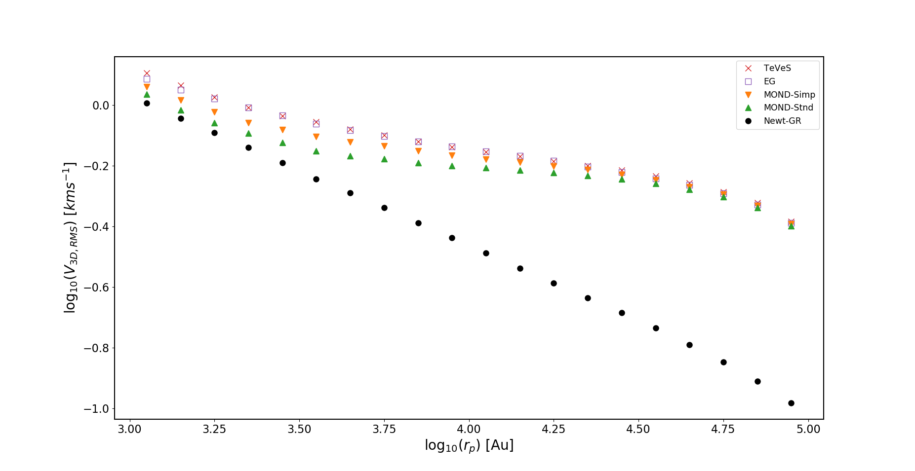
Figure 3: Points show the RMS 3D relative velocity for the set of simulated binary orbits binned in projected separation $r_{p}$; for orbits excluding the external field effect in MOND-like theories. As in the legend, from bottom to top: black circles show Newtonian gravity; upward (downward) pointing triangles show MOND standard (simple) interpolating function respectively; open squares show emergent gravity; crosses show TeVeS.

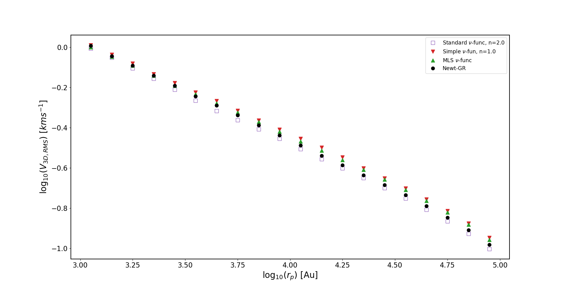
Figure 4: Points show the RMS 3D relative velocity for the set of simulated binary orbits binned in projected separation $r_{p}$; for orbits including the external field effect all with $g_{ext}=1.0\,a_{0}$. As in the legend, black points show Newtonian gravity; open squares show MOND standard interpolating function; downward-pointing triangles show MOND simple interpolating function; upward-pointing triangles show MLS interpolating function.

Turning to the histograms of $v_{3D}/v_{c}(r_{p})$, we find that Newtonian gravity predicts that the histogram of $v_{3D}/v_{c}(r_{p})$ for wide binaries should exhibit a steep decline above values $\sim 1.1$, with an 80th percentile near 1.02 and a 90th percentile near 1.14; these features have rather weak dependence on the poorly known distribution of orbit eccentricities.

In Figures 7 to 7 we show histograms of $v_{\rm 3D}/v_{C}(r_{p})$ in several selected bins of projected separation, comparing Newtonian/GR gravity and various modified-gravity theories without the EFE. It is clear from these that all modified-gravity theories without the EFE produce a large and obvious shift in the distribution, with the 90th percentile reaching $\sim 2.0$ in the projected separation bin $(5,7.1)\,{\rm kAU}$. The specific size of the shift is slightly dependent on the modified-gravity model considered, but all the modified-gravity models without EFE show large shifts: such large effects should be readily detectable by observations, and not reasonably produced by any combination of observational error or sample contamination. We thus conclude that essentially all modified-gravity theories without an EFE can be robustly tested or ruled out by GAIA wide-binary samples with ground-based radial velocity followup.

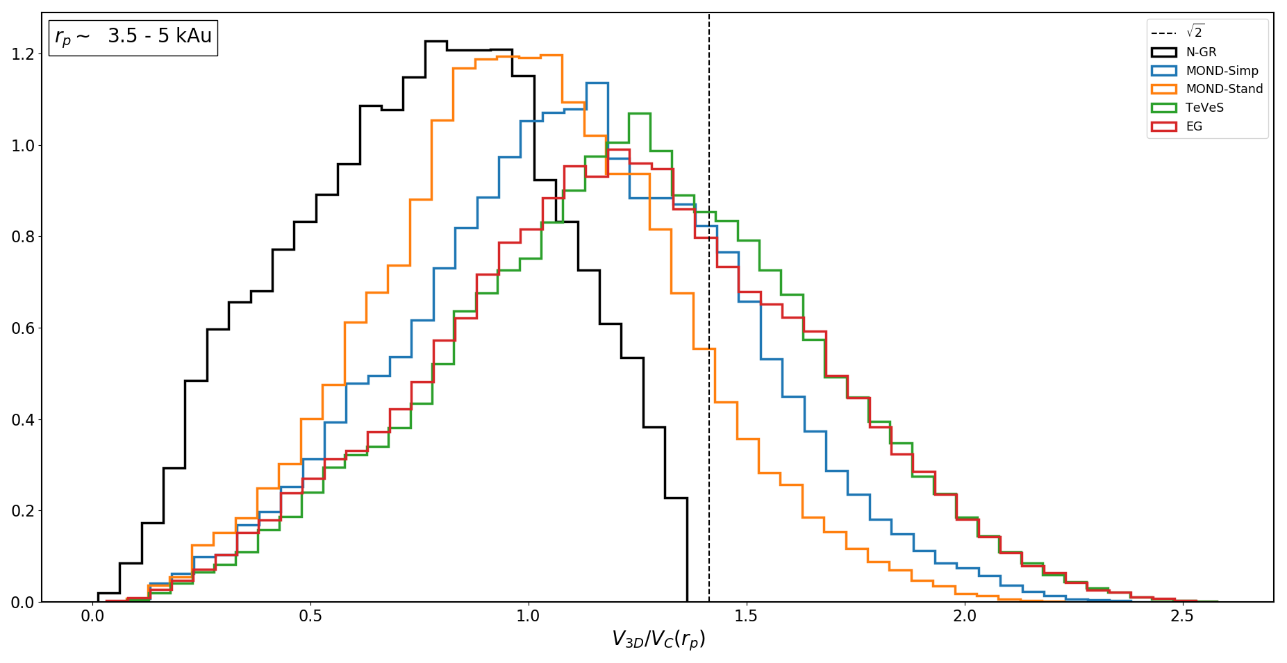
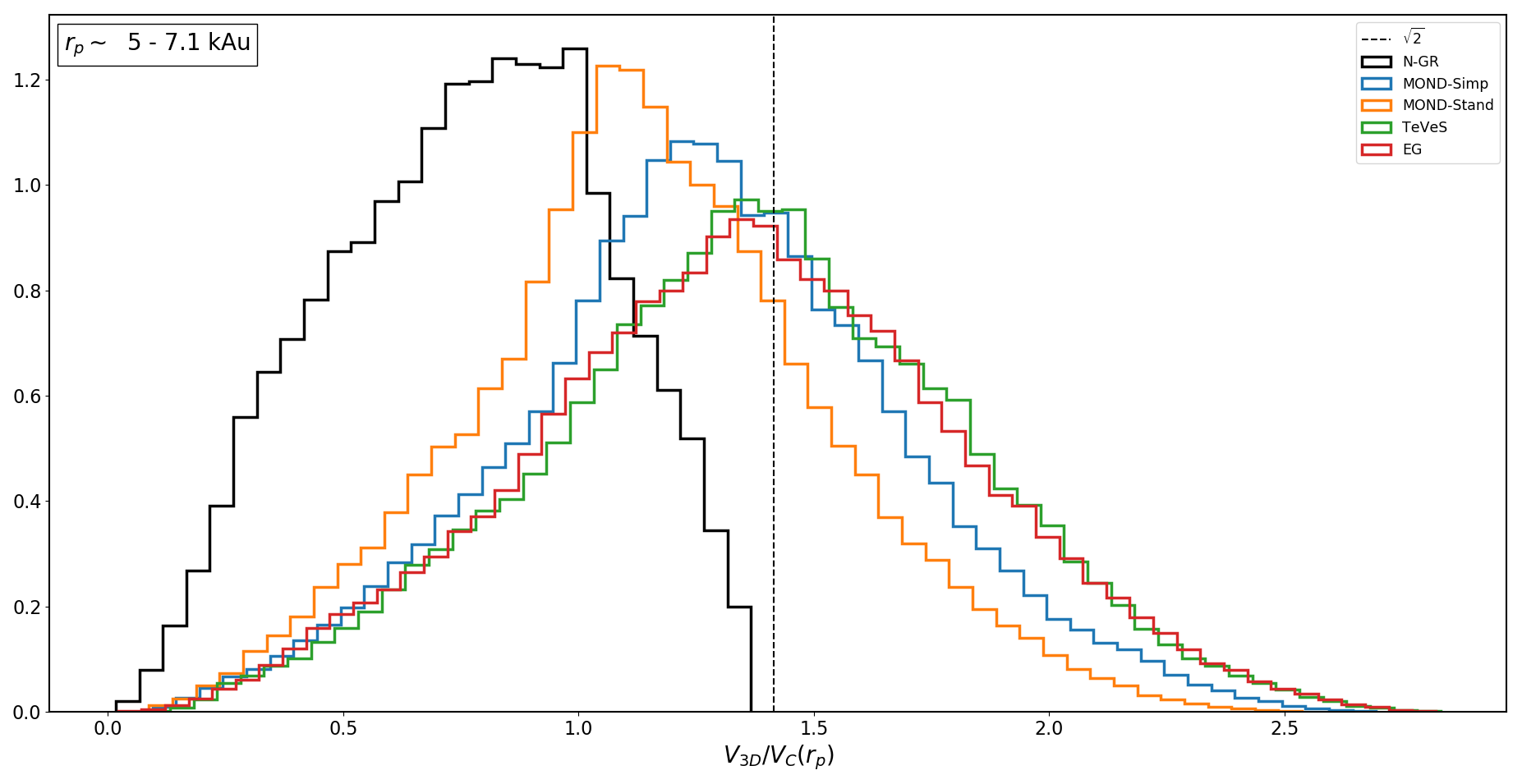
Figure 5: Histogram of simulated $v_{\rm 3D}/v_{C}(r_{p})$ for projected separation range $r_{p}\in(3.5,5)\,{\rm kAU}$, for various gravity models without EFE: Newtonian (black), MOND-simple (blue), MOND-standard (orange), TeVes (green), Emergent gravity (red).

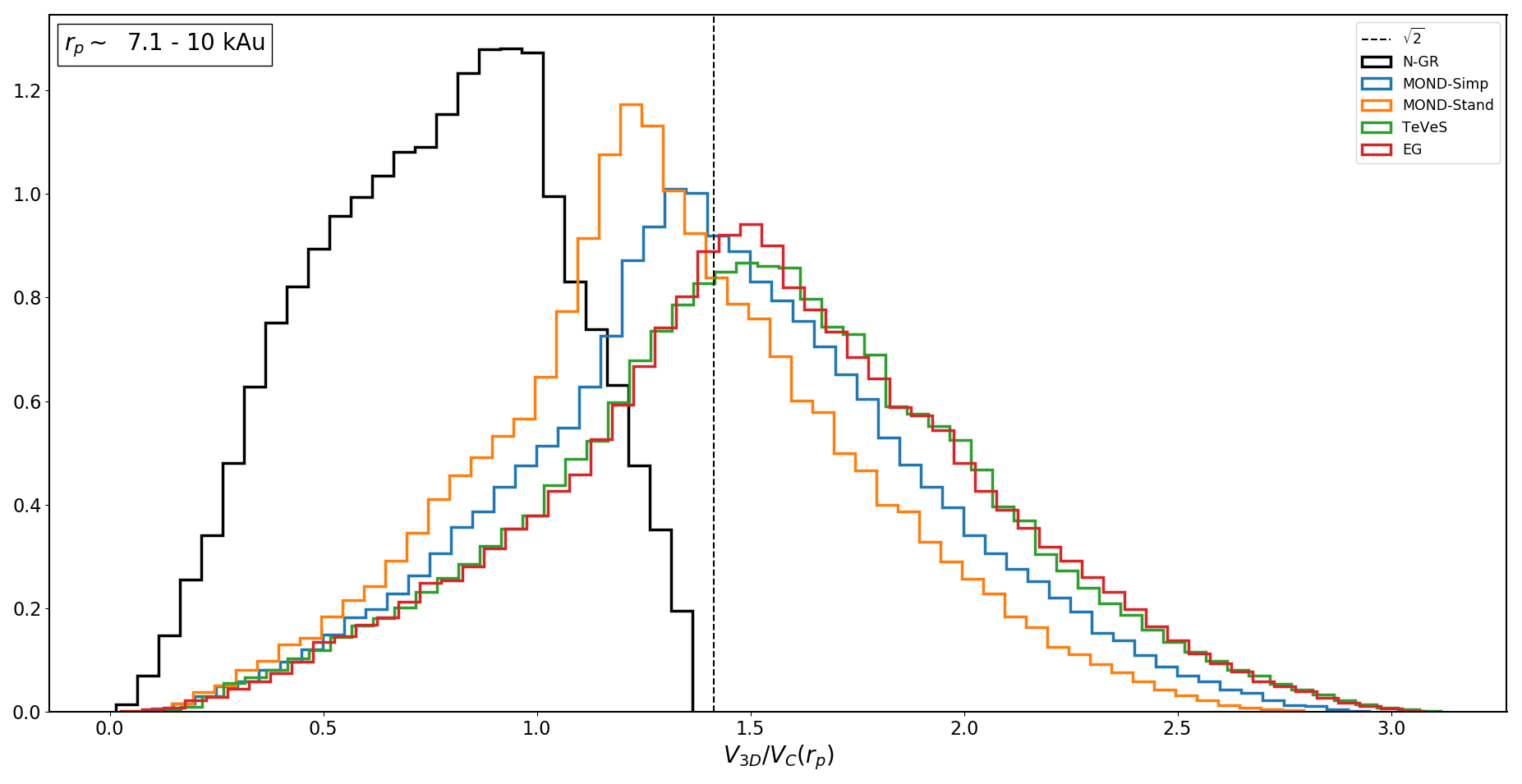
Figure 6: As Figure 7 for projected separation range $r_{p}\in(5,7.1)\,{\rm kAU}$.

Figure 7: As Figure 7 for projected separation range $r_{p}\in(7.1,10)\,{\rm kAU}$.

The next set of Figures show some modified-gravity models with the EFE included: Figures 10 to 10 show results for MOND with the Simple interpolation function for different values of external field, $g_{e}=(0.0,0.5,1.0,1.5)a_{0}$ respectively; so the $g_{e}=0$ case reproduces that from the preceding Figures.

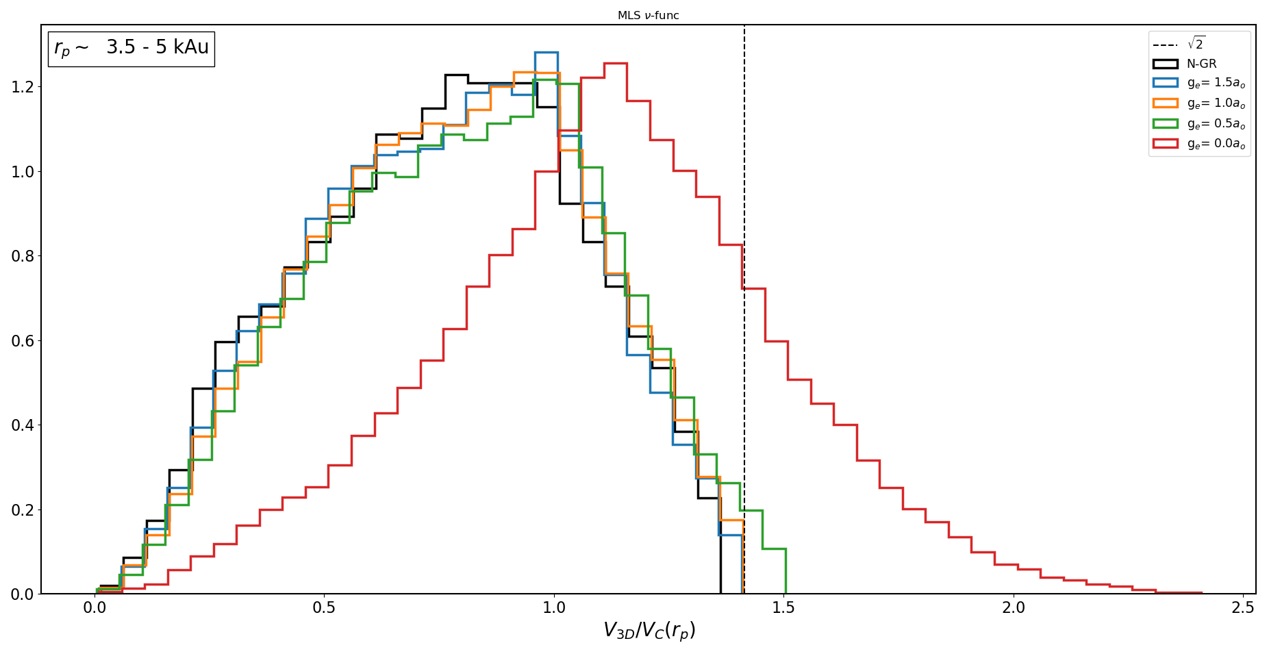
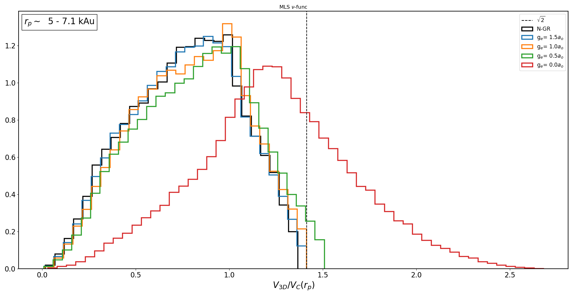
Figure 14: Histogram of simulated $v_{\rm 3D}/v_{C}(r_{p})$ for MLS interpolating function, with EFE, for projected separation range $r_{p}\in(3.5,5)\,{\rm kAU}$. Black histogram is for standard Newtonian gravity, and coloured histograms are for MLS interpolating function including EFE with four values of external field $g_{Ne}$: $g_{Ne}=0$ (red), 0.5 (green), 1.0 (yellow) and 1.5 (blue) in units of $a_{0}$.

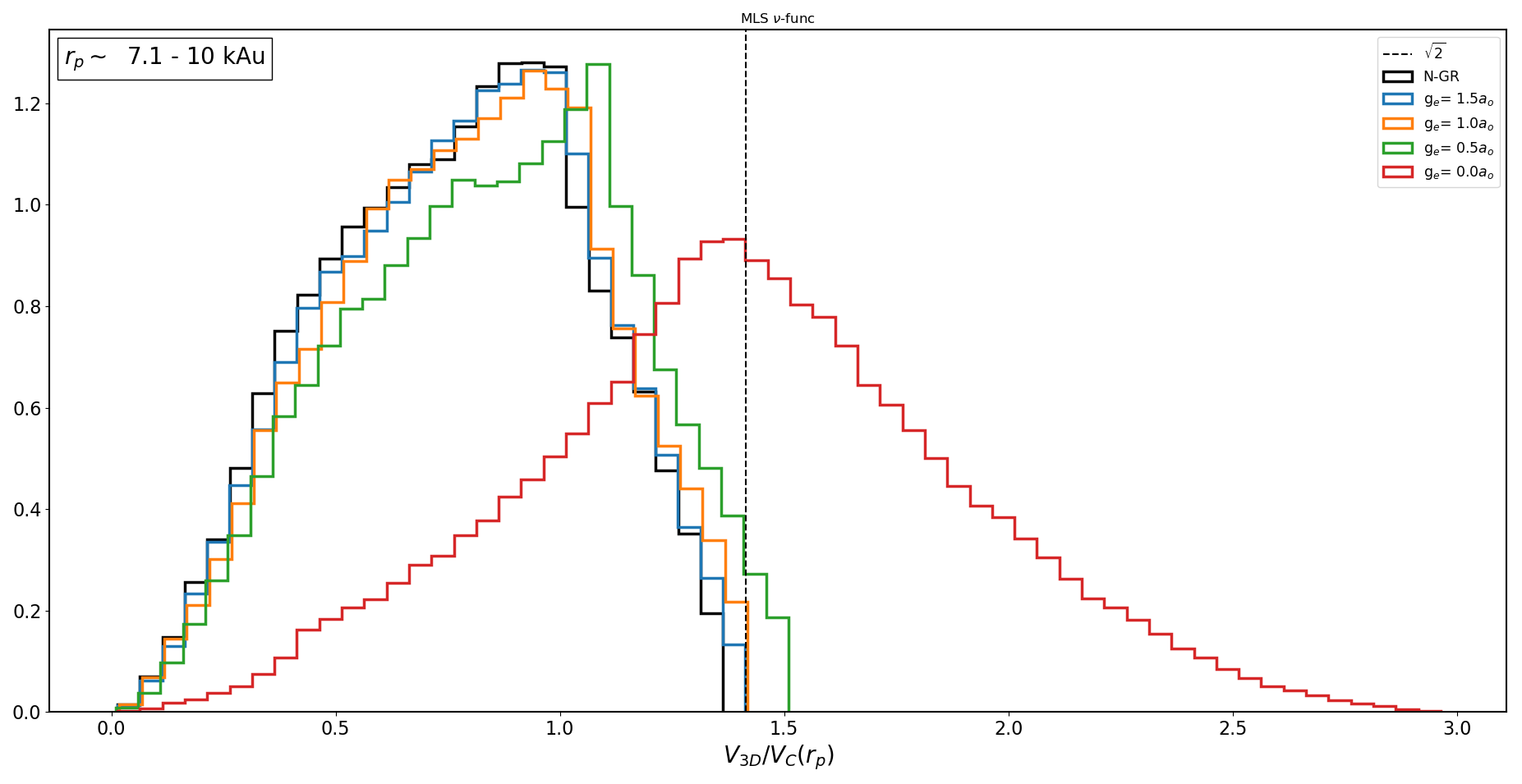
Figure 15: As Figure 16 for projected separation range $r_{p}\in(5,7.1)\,{\rm kAU}$.

Figure 16: As Figure 16 for projected separation range $r_{p}\in(7.1,10)\,{\rm kAU}$.

Likewise, Figures 13 to 13 show the same bins and $g_{e}$ values for the case of the MOND standard interpolating function, while Figures 16 to 16 show the same bins and $g_{e}$ values for the MLS interpolating function of Eq. 42.

It is seen from these figures that with the EFE included, the shifts in the distributions (relative to Newtonian) are considerably smaller than the no-EFE cases, but the shifts remain non-negligible. The shifts are only marginally visible on the histograms, but the shifts particularly in the upper percentiles of the distribution remain non-negligible. For the case $g_{Ne}=1.0\,a_{0}$, we show the resulting 80th and 90th percentile values in Figure 17. These reveal that there are offsets relative to Newtonian gravity by approximately 0.04 to 0.08 in these percentiles, depending on the MOND function, with the offset increasing slowly with separation.

In essence these offsets occur because the EFE leads to approximately a moderate re-normalisation of the effective $G$ at low accelerations: i.e. with the EFE included and external acceleration $g_{Ne}\sim 1\,a_{0}$, the ratio $g_{i}/g_{Ni}$ is slowly varying with scale but is different from 1 at accelerations $\la a_{0}$, so the EFE leads to approximately quasi-Newtonian gravity but with a re-scaled apparent value $G_{\rm eff}$ of the gravitational constant. The limiting ratio $G_{\rm eff}/G_{N}$ is dependent on the choice of MOND interpolating function and the selected value of $g_{e}$.

For the “simple” MOND interpolation function Eq. 40 and $g_{e}=1\,a_{0}$, we find an upward shift of about 7 percent in the 80th and 90th percentile values.

For the MLS interpolation function Eq. 42, the shift is slightly smaller than the MOND-simple interpolation function, with about 4 percent shift; this is in the direction expected since the MLS interpolation function with external $g_{e}=1\,a_{0}$ predicts $g_{i}/g_{N}\sim 1.09$ for $g_{i}\la 1a_{0}$.

There is a somewhat unexpected result from the EFE using the “standard” MOND interpolation function Eq. 41; here the shift is smaller, but actually in the opposite sense i.e. the 80th and 90th percentiles for $v_{\rm 3D}/v_{C}(r_{p})$ are shifted to marginally smaller values than the Newtonian case. This rather counter-intuitive result is actually caused by an odd “feature” of the standard interpolating function including the EFE: in the regime where $g_{e}\approx 1\,a_{0}$ and $g_{i}\la 1\,a_{0}$, the EFE with the standard interpolating function actually predicts internal accelerations $g_{i}$ about 7 percent weaker than Newtonian, $g_{i}/g_{Ni}\sim 0.93$, and this fractional suppression is rather slowly varying for $g_{Ni}$ between 0 to $1\,a_{0}$.

Another point of note is that the shift in the distributions generally becomes apparent at projected separations somewhat smaller than simply the scale $\sim 7\,{\rm kAU}$ where the circular-orbit acceleration is comparable to the MoND $a_{0}$ constant. This occurs for a combination of two reasons: partly because MOND-like effects are expected to become non-negligible at internal accelerations somewhat larger than $1\,a_{0}$ (as preferred to give near-flat galaxy rotation curves and a reasonably smooth interpolation function); and also because the tail of binaries with larger values of $v_{\rm 3D}/v_{C}(r_{p})\ga 1$ is dominated by moderately eccentric orbits which happen to be observed near pericenter: therefore at a given projected separation $r_{p}$, the faster binaries are those with time-average separation larger than the present-day value, hence their past orbit has mainly sampled wider separations where the MOND-like effects are relatively larger.

This feature is interesting, since it implies that MOND-like effects should already start to become measurably large at projected separations $\sim 3-5\,{\rm kAU}$, a range where the survival probability for wide binaries is predicted to be high, the perspective-rotation effects (Section 2.4) are smaller, and the relative velocities are not very small; all of these are favourable from an observational perspective.

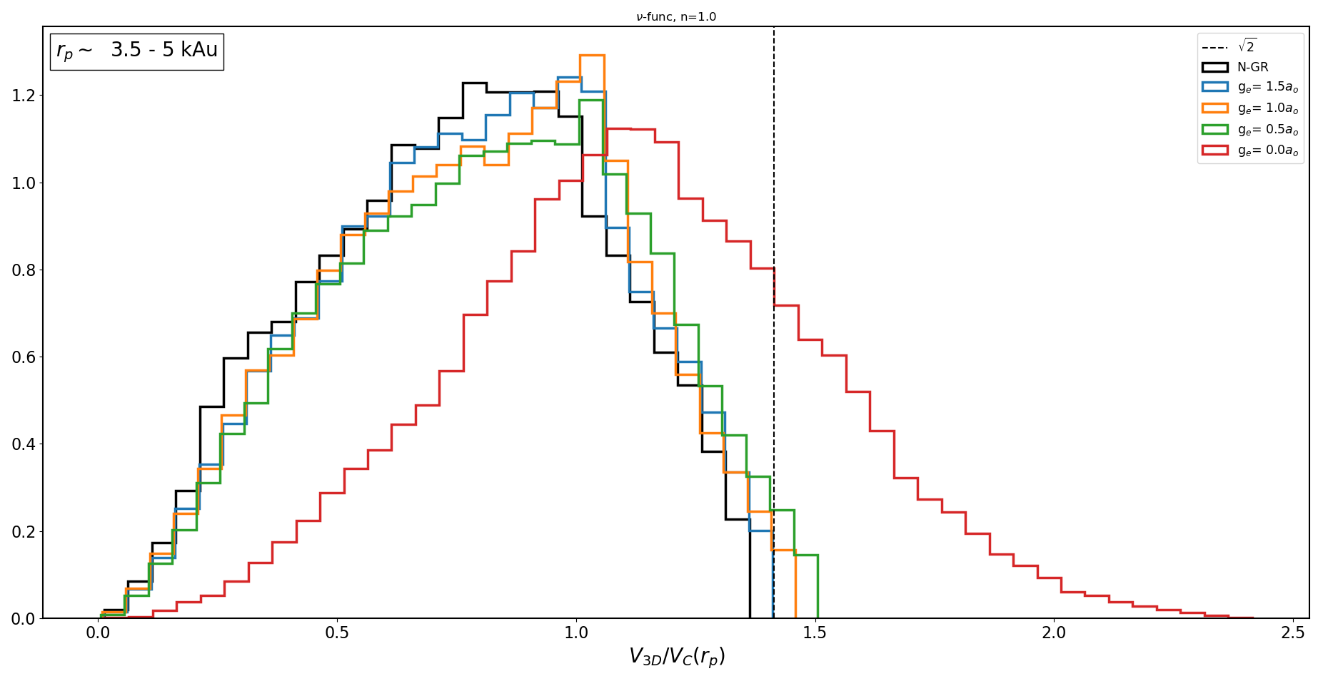
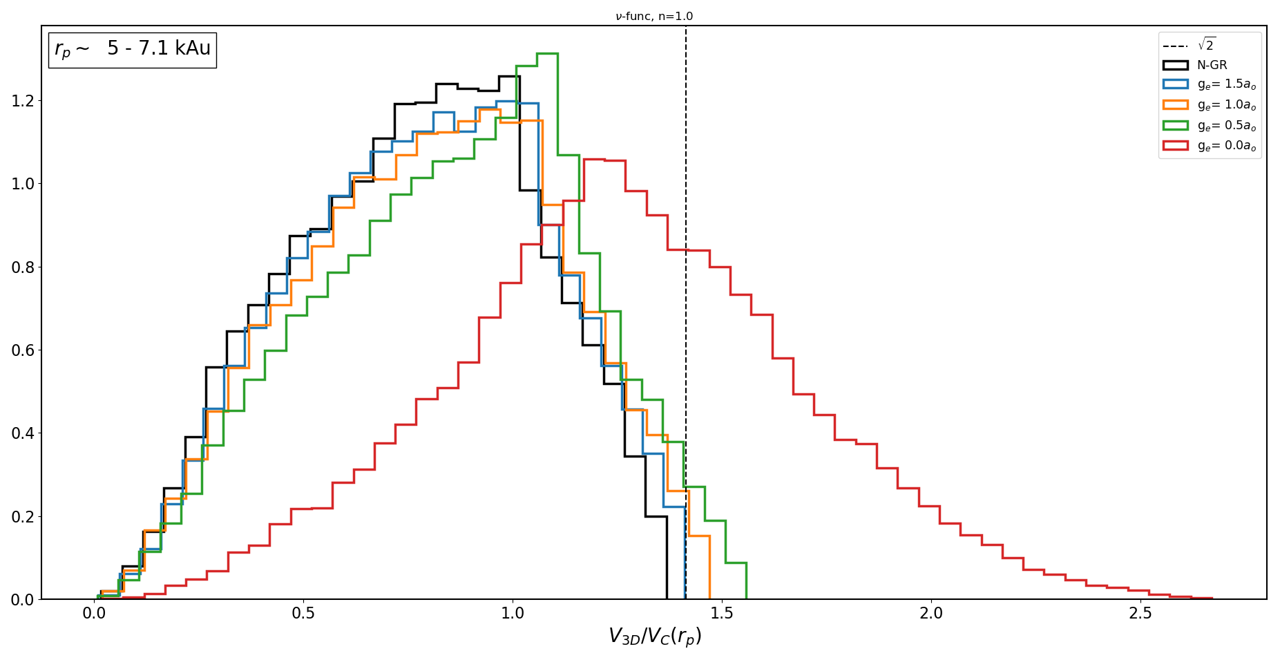
Figure 8: Histogram of simulated $v_{\rm 3D}/v_{C}(r_{p})$ for MOND-simple interpolating function, with EFE, for projected separation range $r_{p}\in(3.5,5)\,{\rm kAU}$. Black histogram is for standard Newtonian gravity, and coloured histograms are for MOND simple interpolating function including EFE with four values of external field $g_{Ne}$: $g_{Ne}=0$ (red), 0.5 (green), 1.0 (yellow) and 1.5 (blue) in units of $a_{0}$.

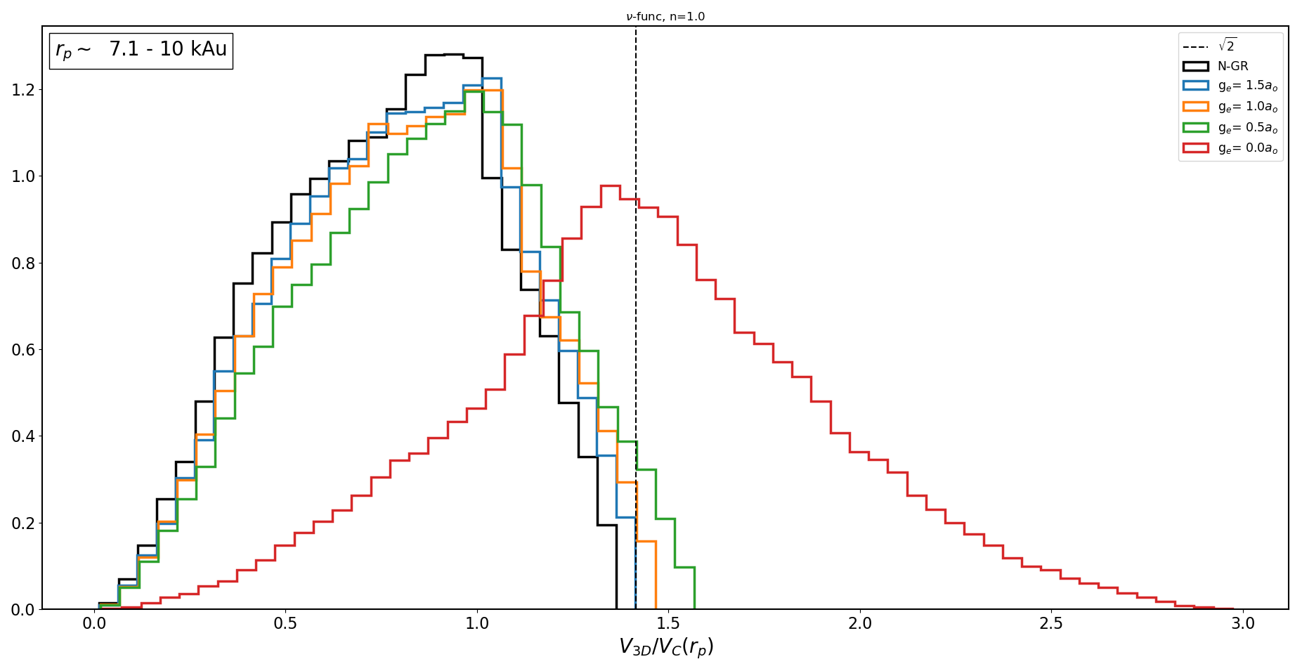
Figure 9: As Figure 10 for projected separation range $r_{p}\in(5,7.1)\,{\rm kAU}$.

Figure 10: As Figure 10 for projected separation range $r_{p}\in(7.1,10)\,{\rm kAU}$.

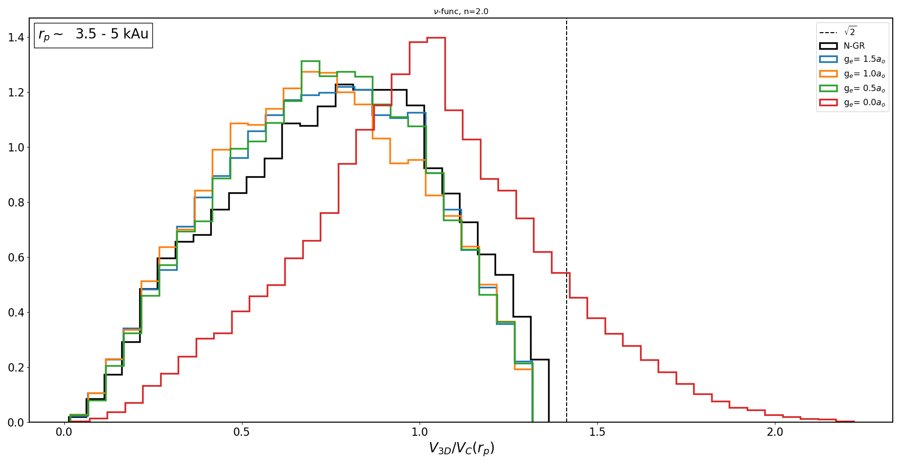
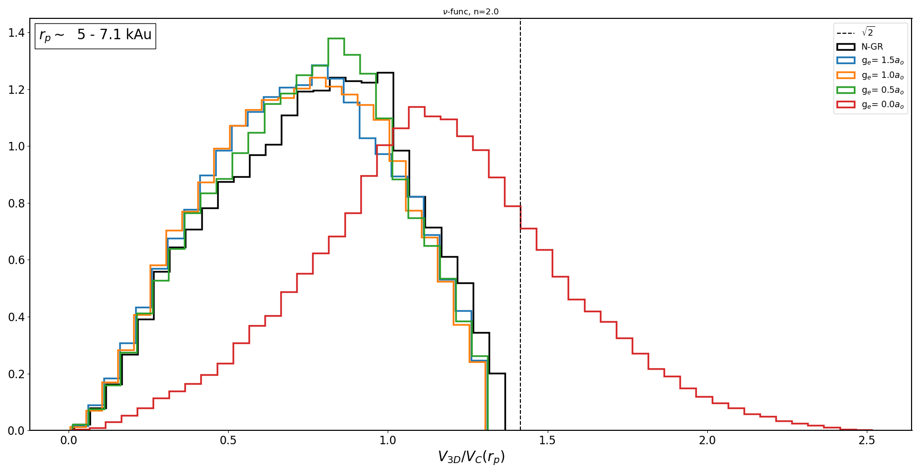
Figure 11: Histogram of simulated $v_{\rm 3D}/v_{C}(r_{p})$ for MOND-standard interpolating function, with EFE, for projected separation range $r_{p}\in(3.5,5)\,{\rm kAU}$. Black histogram is for standard Newtonian gravity, and coloured histograms are for MOND standard interpolating function including EFE with four values of external field $g_{Ne}$: $g_{Ne}=0$ (red), 0.5 (green), 1.0 (yellow) and 1.5 (blue) in units of $a_{0}$.

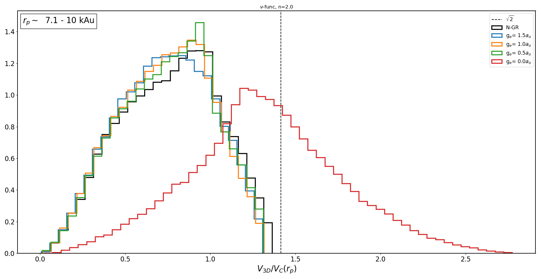
Figure 12: As Figure 13 for projected separation range $r_{p}\in(5,7.1)\,{\rm kAU}$.

Figure 13: As Figure 13 for projected separation range $r_{p}\in(7.1,10)\,{\rm kAU}$.

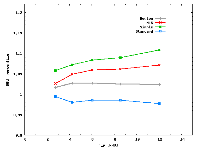
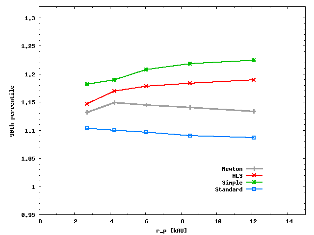
Figure 17: Upper panel: the 80th percentile values of $v_{\rm 3D}/v_{C}(r_{p})$ versus projected separation $r_{p}$ for Newtonian gravity, and three MOND-like models including EFE with external acceleration $G_{Ne}=1\,a_{0}$: the Simple interpolating function (topmost), MLS interpolating function (second from top) and Standard interpolating function (bottom).
Lower panel: the same for the 90th percentile.

The observed shifts in the relative-velocity percentiles (relative to Newtonian values) are qualitatively as expected from the various MOND acceleration laws including the EFE, which behave roughly as a renormalisation of the gravitational constant by a factor which is $\sim 0.9-1.3$ at low accelerations but converge back to 1 at $g_{i}\gg a_{0}$; this factor is generally quite slowly-varying over the range $0.3\,a_{0}<g_{i}<2\,a_{0}$ of interest here, so the relative offset is only slowly varying with binary projected separation and there is no sudden feature at a specific projected separation.

We also find that exploring various choices of interpolation function and different values of the ratio $g_{e}/a_{0}$, that the above rescaling factor is considerably sensitive to both the choice of interpolation function and the numerical ratio of external acceleration $g_{Ne}/a_{0}$, with the deviations increasing for smaller $g_{Ne}/a_{0}$. We note that the TeVeS-like $\mu$ function (Eq. 43) produces relatively larger deviations than the others.

4.3 The QUMOND formulation

After submission of the original version of this paper, we became aware of the work of Banik & Zhao (2015) and Banik & Zhao (2018a); the latter concerns tidal streams rather than binaries, but is also relevant to the case of wide binaries as follows. The QUMOND formulation was introduced by Milgrom (1983) as a simplification of the earlier aquadratic Lagrangian (AQUAL) approach; using QUMOND, Banik & Zhao (2015) give a semi-analytic solution for the acceleration due to a point mass embedded in a tidal field. Banik (private communication) has supplied us with an example set of solutions for several MOND interpolating functions, and the result is that the deviations above Newtonian gravity are rather larger than those adopted above using approximation (45): therefore, a numerical application of the QUMOND formulation to wide binaries is likely to predict larger MOND effects and easier detectability compared to the estimates here and below. Very recently a preprint has appeared by Banik & Zhao (2018b), with a rather detailed simulation of wide binaries in QUMOND with the simple interpolating function; this indeed produces substantially larger MOND deviations than we found here with approximation (45).

5 Observational considerations

We have seen above that without the EFE, we predict rather large and easily detectable shifts; however with the EFE turned on (as generally expected), the shifts due to modified-gravity are relatively small, so it would clearly be necessary to obtain a rather large sample of wide-binary systems in order to get useful statistics. We next make an approximate estimate of the number of useful wide-binary systems as a function of limiting magnitude and distance, to verify that GAIA should produce a large enough sample that the purely statistical errors are small enough, subject to controlling all systematics.

For the present purposes we are mainly interested in binaries where both components are main-sequence stars of spectral type late-F, G, K and early-M (approximately $1.2\,M_{\odot}$ to $0.5\,M_{\odot}$) since brighter stars have few metal lines for precise RV’s, while stars below about $0.5\,M_{\odot}$ are intrinsically faint and hence observationally more challenging.

5.1 Number of wide-binary systems

Here we use the luminosity function (LF) of Chabrier (2003) and the binary separation distribution from Andrews et al. (2017) to estimate the number of suitable systems as a function of apparent magnitude, $V$, distance to system, $d$, and separation of the stellar binary, $s$.

The mass function of Chabrier (2003) results in a local number density 0.0166 stars $\,{\rm pc}^{-3}$ with $0.6\leq M/\,M_{\odot}\leq 1.2$, a range well suited for precision radial velocities. Assuming a $300\,{\rm pc}$ disk scale-height and adding a requirement $V<15$ gives an estimate of total $\sim 196,000$ such stars within $D<150\,{\rm pc}$, or $\sim 394,000$ within 200 pc, where the distance threshold is chosen for good GAIA transverse velocity precision; of course, only a small fraction of those will be members of wide-binary systems of interest here.

The distribution in orbital separations has been estimated recently by Andrews et al. (2017), who determined that the distribution in projected separation $s$ is consistent with the traditional Opik law $s^{-1}$ (i.e. flat in $\ln s$) up to $s\la 5\,{\rm kAU}$, with evidence for a break to a steeper power-law $p(s)\propto s^{-1.6}$ at separations $s\geq 5\,{\rm kAU}$. If we assume that this broken power-law applies from $0.03\,{\rm AU}$ to $100\,{\rm kAU}$, and normalise so that 50 percent of FGK stars have a binary companion anywhere in that range, this predicts that 5.5 percent of FGK stars have a companion star in our range of interest $3<s<20\,{\rm kAU}$; the results of Lepine & Bongiorno (2007) suggest a slightly higher fraction. A significant minority of the secondaries will be mid-M or late-M stars and thus too faint for practical RV followup, but we estimate that $\sim 3$ percent of the above FGK stars should have a usable binary companion at $3<s<20\,{\rm kAU}$ and $V\leq 15$.

Combining the above leads to an approximate estimate of about 5000 potentially usable wide-binary systems (for $D<150\,{\rm pc}$, $V<15$), or over 10,000 if we extend to $D<200\,{\rm pc}$; these are divided between about five separation-bins as used above, so around 1,000 to 2,000 systems per $\sqrt{2}$ separation bin.

5.2 Observational caveats

For binaries in our considered range $V\la 15$, $d\leq 200\,{\rm pc}$, the GAIA statistical proper-motion errors are $\la 0.02{\rm\,km\,s^{-1}}$, and in principle modern planet-hunting spectrographs such as HARPS and ESPRESSO can readily reach differential RV precision well below $0.01{\rm\,km\,s^{-1}}$ at $V\sim 15$. Stellar RV jitter is also usually negligible at these levels, so in principle the binary relative velocities are measurable at better than the 10 percent level.

However, other sources of error are potentially more serious: here we discuss some observational considerations regarding absolute velocity precision, contamination by unbound pairs, and confusion from hierarchical triple/quadruple systems. Our method does rely on a rather good calibration of the luminosity-mass relation. However, this is potentially testable using the binaries at smaller projected separation $\la 1\,{\rm kAU}$ where the deviations due to modified gravity are predicted to be nearly negligible. Also, the required high-quality spectra (for radial velocities) should provide precise metallicities, allowing this to be included in the calibration.

Concerning the absolute velocity precision, while modern high-stability planet-search spectrographs can routinely deliver radial velocity precision $\sim 0.001\,{\rm km\,s^{-1}}$, this however is the differential precision over time for the same star; while here we are interested in the absolute RV difference between the two components of a wide binary. This implies that unlike the planet-finding case, extra systematic effects such as gravitational redshift, convective blueshift, and zeropoint errors from spectral mismatch (actually the difference in these between the two stars) must be corrected for. The gravitational redshift term is $\simeq 0.633{\rm\,km\,s^{-1}}(M/R)$ in solar units, and since the $M/R$ relation is fairly close to linear this is slowly varying for main-sequence stars. This should probably be correctable at better than the $0.03{\rm\,km\,s^{-1}}$ level.

The convective-blueshift term (arising from rising/falling cells of differing temperatures in the stellar atmosphere) is somewhat more challenging, with amplitude estimated as $\simeq-0.3{\rm\,km\,s^{-1}}$ for the Sun and decreasing towards low-mass stars (Kervella et al., 2017). However in practice this term is calibrated out when RVs are zeropointed to the Sun, but re-appears for stars of non-Solar-like spectrum. This term is probably the most important systematic effect in limiting the absolute accuracy on radial velocities; however, the potential bias can be reduced by either selecting subsamples of binaries of similar spectral type, or tested by studying the asymmetry of binary RV differences vs spectral type, since the orbital velocity differences should on average be symmetrical around zero.

It is also possible to use short-period binaries to test for systematic offsets in absolute radial velocity zero-point as a function of spectral type: for short-period binary stars, the time-average of the two radial velocities averaged over an integer multiple of the period should both be equal to the barycentre radial velocity. Thus, observations of medium-separation binary stars with known moderate-period orbits and selected spectral types can potentially provide a check for type-dependent shifts in the RV zeropoint.

Hierarchical triple/quadruple systems where one or both components of the wide system are themselves close binaries are a more serious issue, since for unequal masses (thus very unequal luminosities) the extra components may lurk undetected and can greatly shift the observed relative velocities of the wide system compared to the value for an isolated binary. However, we estimate that this source of contamination should usually be removable by follow-up observations: in the case of very close inner pairs $\la 3\,{\rm AU}$ these should show large radial-velocity variations within a timespan of a year or two; while wider systems $\ga 3\,{\rm AU}$ should be resolvable by direct imaging with adaptive optics unless the extra companion is very faint. This leaves intrinsically faint brown-dwarf or super-Jupiter companions with periods of order 10-100 years as the main potential problem. The brown-dwarf “desert” is helpful in this respect, as cold Jupiters only produce small reflex motions of order $0.012{\rm\,km\,s^{-1}}$, while brown dwarfs above the D-burning limit should mostly be detectable in deep imaging.

Contamination from unbound pairs misclassified as bound binaries is a potentially more serious issue: however, we note that for a random phase-space distribution the contamination should be very small. For objects with a density of order $0.1\,{\rm pc}^{-3}$ and velocity dispersion $\sim 25{\rm\,km\,s^{-1}}$, the probability for a given primary star to have a chance-flyby companion with projected separation $r_{p}<30\,{\rm kAU}$, radial separation $\Delta d<0.5\,{\rm pc}$ and 3D velocity difference $\leq 1{\rm\,km\,s^{-1}}$ is of order $10^{-6}$, which is far below the estimated fraction of true wide binaries. This leaves the major issue as objects with correlations in phase-space: either “ionized” previously-bound wide binaries, or unbound pairs with a common origin, are the main potential source of contamination. Most of these are expected to have $v_{3D}/v_{c}(r_{p})\ga 2$ and these can be clipped from the sample; the remaining issue is that unbound common-origin pairs aligned at a relatively small angle to the line-of-sight (small $\sin\beta$) can then masquerade as bound binaries with $v_{3D}/v_{c}(r_{p})\sim 1.1$, hence causing an upward bias in the 80th or 90th percentile value for apparently-bound binaries. It should be possible to model the distribution of these by counting unbound pairs as a function of projected separation and velocity difference and assuming random viewing angles, though this will require further study; this is beyond the scope of the present work.

Thus it appears that none of the above problems is serious enough to be a fundamental blocker from an observational perspective, though they may substantially increase the requirements in follow-up observing time to eliminate hierarchical triple/quadruple systems, to check for spectral-type-dependent offsets in the RV zeropoint, and to check the mass-luminosity relation using smaller-separation binaries.

5.3 Statistical errors

Here we note that the steep fall in the histogram of relative velocities at $v_{3D}/v_{C}(r_{p})\sim 1.1$ is also helpful for statistics: this implies that the statistical uncertainty in estimating the 80th and 90th percentiles from a sample size of $N$ binaries is substantially smaller than the naive estimate $\approx 1/\sqrt{N}$; in essence this arises because detecting a “sharp edge” in a distribution is more precise than estimating the centroid of a broad distribution.

For example, if we define $X_{90}$ to be the observed 90th percentile from a sample of $N$, and $x$ is an arbitrary variable, then $P(X_{90}>x)$ can be calculated as the binomial probability of obtaining $\geq 0.1N$ “successes” from $N$ independent trials with probability $1-C(x)$, where $C(x)$ is the cumulative PDF for one binary. Then, for an example case of $N=1000$, we expect $100\pm\sqrt{90}$ binaries above the true 90th percentile, hence there is just over 68% probability that the observed 90th percentile will fall between the true 89th and 91st percentiles; from the simulated histograms above, these points are offset by $\simeq\pm 0.01$ from the 90th percentile. Thus the uncertainty on the 90th percentile should be reasonably approximated by $0.3/\sqrt{N}$, not simply $1/\sqrt{N}$. This implies that a sample of $\sim 1000$ well-measured binaries can give a statistically significant detections of an offset $\sim 0.04$ relative to Newtonian predictions, which is enough to robustly detect the offsets predicted in MOND-like modified gravity models, even in the various EFE cases, if all systematic errors and contamination can be controlled well enough and/or statistically corrected via simulations.

6 Conclusions

Following on from earlier related studies (e.g. Hernandez et al. (2011), Hernandez et al. (2012), Hernandez et al. (2017)), we have estimated the prospects for observational tests of modified-gravity theories using wide-binary stars selected by GAIA and high-precision radial velocities from ground-based telescopes. Considering the ratio of 3-D relative velocities to the Newtonian circular velocity, in standard gravity the probability distribution function contains a rather steep decline at $v_{3D}/v_{C}(r)\sim 1.2$, resulting in 80th and 90th percentile values which are only weakly dependent on the uncertain distribution of orbital eccentricities. In a practical case we only have access to projected separation $r_{p}$ rather than $r$, but this causes only a modest broadening of the distribution towards smaller values of the ratio $v_{3D}/v_{C}(r_{p})$; this parameter is well measurable with GAIA data combined with accurate ground-based RV measurements.

We simulated large numbers of binary orbits with various gravity models observed at random angles and phases, and evaluated the statistical distribution of $v_{3D}/v_{c}(r_{p})$, in particular the 80th and 90th percentile values which are reasonably insensitive to the eccentricity distribution and only weakly sensitive to a small fraction of contaminants.

Our general conclusions are summarised as follows:

1. If the relevant modified-gravity theory does not contain an external field effect, then large non-Newtonian deviations in the relative velocity distribution should be easily observable for binaries wider than about $5\,{\rm kAU}$, so MOND-like theories without an EFE should be rather easy to detect or rule out with samples of a few hundred wide binaries.

2. Binary projected separations of order $3-15\,{\rm kAU}$ seem to be the most promising range, since MOND-like effects should start to appear above a few $\,{\rm kAU}$; while other considerations (required velocity precision, perspective rotation effects, tidal effects) all become more challenging at even larger separations.

3. With the external field effect (EFE) turned on (as in most MOND-like modified gravity theories), the deviations are considerably reduced, but are still potentially detectable and contribute a shift of order $\sim 4-8$ percent, depending on the MOND interpolating function, which is potentially detectable with a moderately large statistical sample of order 1000 well-observed wide-binary systems.

4. Again with the external field effect turned on, the size of deviations predicted by MOND-like theories are quite sensitive to the specific shape of the MOND interpolating function (or equivalent) and the value of the external field. Since the Galactic acceleration field (from baryons) is quite close to $1\,a_{0}$, the wide binaries are in a regime where the Galactic and internal accelerations are rather similar. This implies that MOND-like effects tend to produce an acceleration law with slope fairly close to $1/r^{2}$, but with an apparent rescaling of the gravitational constant.

5. To a reasonable approximation, MOND-like theories including the EFE produce a shift in the 80th and 90th percentiles of $v_{\rm 3D}/v_{C}(r_{p})$ which are proportional to $\sqrt{G_{\rm eff}/G}$ in the relevant MOND model; this allows a qualitative assessment of the effects for other MOND-like models beyond those simulated here.

6. Improved constraints in future on the Galactic acceleration and the required shape of the MOND interpolating function around $\sim 1\,a_{0}$, both from GAIA and external galaxy rotation curves, will be helpful to constrain these and give more specific predictions for the size of deviations.

7. More detailed computations of the MOND accelerations with the Galactic external field as in e.g. Banik & Zhao (2015) and Banik & Zhao (2018b) indicate larger deviations from GR than the approximations we used above; this improves the prospects for observational tests.

8. The sample of observable wide binaries at $d\la 200\,{\rm pc}$ from GAIA is probably large enough to give a statistically significant test for the presence or absence of MOND-like effects, if all systematic errors and contamination can be well controlled or statistically corrected from simulations.

Further study is needed to investigate the practical effects of contamination from common-origin unbound stellar pairs, realistic systematic errors in the luminosity/mass relation, possible radial velocity systematic errors, and perspective-rotation effects; these will probably require considerably more detailed simulations and also more input from future observations, so this paper provides essentially an initial feasibility study.

However, this test looks potentially very interesting as an observationally viable probe of possible modified-gravity effects in a relatively less explored portion of parameter space.

References

- Ade et al. (2016) Ade P. et al. (Planck Collaboration), 2016, A&A, 594, A13. (arXiv:1502.01589)
- Akerib et al. (2017) Akerib D. et al. (LUX Collaboration), 2016, Phys. Rev. Lett., 118, 021303 (arXiv:1608.07648)
- Andrews et al. (2017) Andrews J.J., Chanam J., Ageros M.A., 2017, MNRAS, 472, 675. (arXiv:1704.07829)
- Angelil & Saha (2008) Angelil R., Saha P., 2008, The MOND paradigm: from Law to Theory, source:
- Banik & Zhao (2015) Banik I., Zhao H., 2015, preprint, (arXiv:1509.08457)
- Banik & Zhao (2018a) Banik I., Zhao H., 2018a, MNRAS, 473, 419.
- Banik & Zhao (2018b) Banik I., Zhao H., 2018b, preprint, (arXiv:1805.12273)
- Beech (2011) Beech M., 2011, Ap&SS, 333, 419.
- Bekenstein (2004) Bekenstein J.D., 2004, Phys. Rev. D, 70, 083509. (arxiv:astro-ph/0403694v6)
- Bekenstein & Milgrom (1984) Bekenstein J.D., Milgrom M., 1984, ApJ, 286, 7.
- Benedict et al. (2016) Benedict G.F., Henry T.J., Franz O.G. et al, 2016, ApJ, 152, 141.
- Bernal et al. (2011) Bernal T., Capoziello S., Hidalgo J.C., Mendoza S., 2011, Eur. Phys. Jour. C, 71, 1794
- Boran et al. (2017) Boran S., Desai S., Kahya E., Woodard R., 2017, preprint. (arXiv:1710.06168)
- Capozziello & de Laurentis (2011) Capozziello S., de Laurentis M., 2011, Phys. Rep., 509, 167.
- Chabrier (2003) Chabrier G., 2003, PASP, 115, 763. (arXiv:astro-ph/0304382v2)
- Chaname & Gould (2004) Chanam, J., Gould, A., 2004, ApJ, 601, 289. (arXiv:astro-ph/0307434)
- Coronado & Chaname (2015) Coronado J., Chanam J., 2015. VI Reunion de Astronomia Dinamica en Latinoamerica (ADeLA 2014) (Eds. K. Vieira, W. van Altena & R.A. Mendez), Revista Mexicana de Astronomia y Astrofisica (Serie de Conferencias), 46, 61.
- Clifton et al. (2012) Clifton, T., Ferreira, P. G., Padilla, A., Skordis, C., 2012, Phys. Rep., 513, 1. (arXiv:1106.2476)
- Dai & Stojkovic (2017) Dai D.C., Stojkovic D., 2017, JHEP, 1711, 007.
- Dhital et al. (2010) Dhital S., West A.A., Stassun K.G., Bochanski J., 2010, AJ, 139, 2566.
- Durazo et al. (2017) Durazo R., Hernandez X., Cervantes Sodi B., Sanchez S.F., 2017, ApJ, 837, 179.
- Famaey & Binney (2005) Famaey B., Binney J.J., 2005, MNRAS, 363, 603.
- Famaey & McGaugh (2012) Famaey B., McGaugh S.S., 2012, Living Rev. Relativity 15, 10. (doi:10.12942/lrr-2012-10) (arXiv:1112.3960)
- Hernandez et al. (2011) Hernandez X., Jimenez A., Allen C., 2011, European Phys. J. C, 72, 1884. (arXiv:1105.1873)
- Hernandez et al. (2012) Hernandez X., Jimenez A., Allen C., 2012, Journal of Physics: Conf. Series, 405, 012018. (arXiv:1205.5767)
- Hernandez et al. (2014) Hernandez X., Jimenez A., Allen C., 2014, in “Accelerated Cosmic Expansion”, Astrophys. and Space Sci. Procs., 38, 43 (Springer). (arXiv:1401.7063)
- Hernandez et al. (2017) Hernandez X., Cortes R.A.M., Scarpa R., 2017, MNRAS, 464, 2930.
- Hossenfelder (2017) Hossenfelder S., 2017, Phys. Rev. D, 95, 124018, (arXiv:1703.01415)
- Jiang & Tremaine (2010) Jiang Y.-F., Tremaine S., 2010, MNRAS, 387, 1727. (JT10).
- Kervella et al. (2017) Kervella P., Thevenin F., Lovis C., 2017, A&A, 598, 7.
- Kouwenhoven et al. (2010) Kouwenhoven M.B.N., Goodwin S.P., Parker R.J., Davies M.B., Malmberg D., Kroupa P., 2010, MNRAS, 404, 1835.
- Lepine & Bongiorno (2007) Lepine S., Bongiorno B., 2007, AJ, 133, 889.
- Licquia & Newman (2016) Licquia T.C., Newman J.A., 2016, ApJ, 831, 71. (arXiv:1607.05281)
- Lughausen, Famaey & Kroupa (2014) Lughausen F., Famaey B., Kroupa P., 2014, MNRAS, 441, 2497.
- McGaugh (2008) McGaugh S.S., 2008, ApJ, 683, 137. (arXiv:0804.1314)
- McGaugh et al. (2016) McGaugh S.S., Lelli F., Schombert J.M., 2016, Phys. Rev. Lett.117, 201101. (MLS); (arXiv:1609.05917)
- McMillan (2017) McMillan P., 2017, MNRAS, 465, 76. (arXiv:1608.00971)
- Mendoza et al. (2013) Mendoza S., Bernal T., Hernandez X., Hidalgo J.C., Torres L.A., 2013, MNRAS, 433, 1802.
- Milgrom (1983) Milgrom M., 1983, ApJ, 270, 365.
- Milgrom (1983) Milgrom M., 2010, MNRAS, 403, 886.
- Matvienko & Orlov (2015) Matvienko A.S., Orlov V.V., 2015, Astronomy Letters, 41, 824.
- Penarrubia et al. (2016) Penarrubia J., Ludlow A.D., Chaname J., Walker M.G., 2016, MNRAS, 461, L72.
- Prusti et al. (2016) Prusti T., de Bruijne J.H.J. et al (GAIA collaboration), 2016, A&A, 595, A1.
- Quinn et al. (2009) Quinn D.P., Wilkinson M.I., Irwin M.J. et al, 2009, MNRAS, 396, L11. (arXiv:0903.1644)
- Quinn & Smith (2009) Quinn D.P., Smith M.C., 2009, MNRAS, 400, 2128. (arXiv:0908.3640)
- Scarpa et al. (2017) Scarpa R., Ottolina R., Falomo R., Treves A., 2017, Int. J. Mod. Phys. D, 26, 1750067 (arXiv:1611.08635)
- Shaya & Olling (2011) Shaya E.J., Olling R.P., 2011, ApJS, 192, 2. (SO11); (arXiv:1007.0425)
- Tokovinin & Kiyaeva (2016) Tokovinin A., Kiyaeva O., 2016, MNRAS, 456, 2070. (arXiv:1512.00278)
- Will (1993) Will C.M., 1993, Theory and Experiment in Gravitational Physics, Revised Edition, Cambridge Univ. Press.
- Yoo et al. (2003) Yoo J., Chaname J., Gould A., 2003. ApJ, 601, 311. (arXiv:astro-ph/0307437)
- Verlinde (2016) Verlinde E.P., 2016, preprint (arXiv:1611.02269)