Quadratic Points of Surfaces in Projective $3$-Space

Abstract

Quadratic points of a surface in the projective $3$-space are the points which can be exceptionally well approximated by a quadric. They are also singularities of a $3$-web in the elliptic part and of a line field in the hyperbolic part of the surface. We show that generically the index of the $3$-web at a quadratic point is $\pm 1/3$, while the index of the line field is $\pm 1$. Moreover, for an elliptic quadratic point whose cubic form is semi-homogeneous, we can use Loewner’s conjecture to show that the index is at most $1$.

From the above local results we can conclude some global results: A generic compact elliptic surface has at least $6$ quadratic points, a compact elliptic surfaces with semi-homogeneous cubic forms has at least $2$ quadratic points and the number of quadratic points in a hyperbolic disc is odd. By studying the behavior of the cubic form in a neighborhood of the parabolic curve, we also obtain a relation between the indices of the quadratic points of a generic surface with non-empty elliptic and hyperbolic regions.

1 Introduction

Consider a surface $M$ in $3$-space. A quadratic point $p$ is a point where $M$ can be exceptionally well approximated by a quadric. Generically, the quadratic points are isolated and occur at the elliptic or the hyperbolic region of $M$, not in the parabolic curve.

Examples of algebraic hyperbolic tori in projective $3$-space with many quadratic points can be found in [13], where it is conjectured that any hyperbolic tori in $\mathbb{P}^{3}$ should have quadratic points. In [2] one can find hyperbolic tori in $\mathbb{S}^{3}$ with no quadratic points. In [15], it is proved that any hyperbolic disk bounded by a parabolic curve should have an odd number of quadratic points.

The cubic form $C$ defines a binary cubic differential equation (BCDE) outside the parabolic curve. This BCDE is totally real in the elliptic region and has one root in the hyperbolic region, and is singular exactly at the quadratic points. Thus the cubic form defines a line field ${\mathcal{H}}$ in the hyperbolic region and a $3$-web ${\mathcal{E}}$ in the elliptic region, except at quadratic points. Both fields are projectively invariant.

The behavior of a totally real $3$-web close to a singularity was studied in [3]. Applying the results of this paper to the particular case of a cubic form, we verify that generically the $3$-web $\mathcal{E}$ has index $\pm\frac{1}{3}$ at quadratic elliptic points. As a corollary we have that at a generic compact convex surface, there exist at least $6$ quadratic points.

For semi-homogeneous cubic forms, we show a relation between the index of the $3$-web and Loewner’s conjecture to conclude that the index of a quadratic point is at most $1$. As a corollary, we obtain that, under the semi-homogeneity hypothesis, the number of quadratic points in a compact convex surface is at least $2$, which is a version of Carathéodory conjecture. We also give an example of a compact rotation surface with exactly $2$ quadratic points.

For quadratic points in the hyperbolic region, we show that generically the line field $\mathcal{H}$ has index $\pm 1$. By considering the polar blow-up, we describe the generic phase portrait of $\mathcal{H}$ at these points.

In a neighborhood of the parabolic curve, there exists a line field ${\mathcal{L}}$, tangent to the parabolic curve, which coincides with the line field $\mathcal{H}$ in the hyperbolic part $H$ and with a line field $\mathcal{E}_{1}$ of the $3$-web $\mathcal{E}$ in the elliptic part $E$. With the help of this line field, we prove a version of Poincaré-Hopf Theorem which says that for a generic compact surface $M$ with elliptic region $E$ and hyperbolic region $H$,

$$\sum_{p_{i}\in E}Ind(p_{i},\mathcal{E})+\sum_{p_{i}\in H}Ind(p_{i},\mathcal{H})=\chi(M).$$

where the sum is taken over the the quadratic points $p_{i}$.

The paper is organized as follows: In section 2 we show the relation between quadratic points and cubic forms. In section 3 we study the behavior of the $3$-web $\mathcal{E}$ at a simple quadratic point, while in section 4 we calculate the index of a $3$-web coming from a semi-homogeneous cubic form. In section 5 we study the behavior of the line field $\mathcal{H}$ at a simple quadratic point. In section 6 we calculate the cubic form in a neighborhood of a generic parabolic curve. Finally, in section 7, we prove some Poincaré-Hopf type theorems.

2 Quadratic points and cubic forms

2.1 Darboux directions and quadratic points

A general point $p\in M$ admits a $3$-dimensional space quadrics with contact of order $2$ with the surface, i.e., with the same tangent plane and the same curvatures in all directions. Among these quadrics, there are three one-parameter families with the property that the contact function is a perfect cube. If $p$ is elliptic, all three families are real, while if $p$ is hyperbolic, one of these families is real and the other two complex.The null directions of the perfect cubes are called Darboux directions ([4, p.358], [7, p. 141-144]).

Quadratic points $p\in M$ are points that admits an osculating quadric of order $3$. Quadratic points are invariant by projective transformations of the $3$-space and admit a one-dimensional space of third order osculating quadrics.

Example 1.

Let $p=(0,0,0)$ and $M$ be given by

$$z=\frac{1}{2}(x^{2}+y^{2})+\frac{c}{6}(x^{3}-3xy^{2})+O_{4}(x,y).$$ (2.1)

Any quadric of the form

$$z=\frac{1}{2}(x^{2}+y^{2})+\alpha xz+\beta yz+\gamma z^{2}$$

has a second order contact with $M$ at $p$. For the quadrics

$$z=\frac{1}{2}(x^{2}+y^{2})-cxz+\gamma z^{2},$$

the contact function at order $3$ is a multiple of $x^{3}$. Thus $(0,1)$ is a Darboux direction. The other Darboux directions are $(3,\pm\sqrt{3})$. The point $p$ is quadratic if and only if $c=0$.

Example 2.

Let $p=(0,0,0)$ and $M$ be given by

$$z=xy+a^{3}x^{3}+b^{3}y^{3}+O_{4}(x,y).$$ (2.2)

Any quadric of the form

$$z=xy+\alpha xz+\beta yz+\gamma z^{2}$$

has a second order contact with $M$ at $p$. For the quadrics

$$z=xy-3a^{2}bxz-3ab^{2}yz+\gamma z^{2},$$

the contact function at order $3$ is a multiple of $(ax+by)^{3}$. Thus $(-b,a)$ is the Darboux direction. The point $p$ is quadratic if and only if $a=b=0$.

2.2 Affine differential geometry and cubic forms

In the elliptic and hyperbolic parts of $M$, consider the equation

$$D_{X}Y=\nabla_{X}Y+g(X,Y)\xi$$

where $X,Y$ are vector fields on $M$, $\xi$ is a transversal vector field, $\nabla$ is an affine connection and $g$ a non-degenerate bilinear form. It turns out that there exists a unique (up to sign) vector field $\xi$ such that $D_{X}\xi$ is tangent to $M$, for any vector field $X$ on $M$, and the area form induced by $\xi$ coincides with the area form defined by $g$. This $\xi$ is called the affine normal vector field, the corresponding $g$ and $\nabla$ are called the Blaschke metric and induced connection, respectively. At elliptic points, the Blaschke metric is definite, while at hyperbolic points, the Blaschke metric is indefinite (see [8]).

The cubic form in the elliptic and hyperbolic parts of $M$ are defined by $C=\nabla g$. It turns out that the conformal class of the cubic forms is projectively invariant. At elliptic points, $C$ has three real null directions, while at hyperbolic points, $C$ has only one real null direction (see [8]). The following result can be found in [12, p.114]:

Lemma 2.1.

A point $p$ is quadratic if and only if $C(p)=0$.

Proof.

Assume first that $p$ is elliptic. Then, up to an affine change of coordinates, the surface $M$ in a neighborhood of $p$ is given by equation (2.1). Then $p$ is quadratic if and only if $c=0$, i.e., if and only if the cubic form at $p$ is zero.

If $p$ is hyperbolic, up to an affine change of coordinates, the surface $M$ in a neighborhood of $p$ is given by equation (2.2) The point $p$ is quadratic if and only if $a=b=0$, i.e., if and only if the cubic form at $p$ is zero. ∎

3 Simple quadratic points in the elliptic region

Assume that $M$ is the graph of $f:U\subset\mathbb{R}^{2}\to\mathbb{R}$ given by

$$f=\frac{1}{2}(x^{2}+y^{2})+\frac{1}{24}\left(a_{40}x^{4}+4a_{31}x^{3}y+6a_{22}x^{2}y^{2}+4a_{13}xy^{3}+a_{04}y^{4}\right)+O_{5}(x,y),$$ (3.1)

where $O_{5}(x,y)$ denotes the terms of order $\geq 5$ in $(x,y)$. Then the cubic form is given by

$$\omega=\omega_{1}+O_{2}(x,y),$$ (3.2)

where

$$\omega_{1}=(ax+by)(dx^{3}-3dxdy^{2})+(cx+dy)(dy^{3}-3dydx^{2})$$ (3.3)

and

$$a=a_{40}-3a_{22},\ b=a_{31}-3a_{13},\ c=a_{13}-3a_{31}\ d=a_{04}-3a_{22},$$ (3.4)

(see appendix A). We say that the singularity $(0,0)$ of $\omega$ is simple if it is also an isolated singularity of $\omega_{1}$. It is easy to check that this condition is equivalent to

$$ad-bc\neq 0.$$ (3.5)

Observe that for a generic surface $M$, all quadratic points are simple.

3.1 Index of simple quadratic points

Using complex notation we can write $\omega=(A+iB)dz^{3}+(A-iB)d\bar{z}^{3}$, where $A=C_{111}$ and $B=C_{222}$. It is proved in [3] that the index $I=I(0,0)$ of the singularity is given by

$$I=-\frac{\deg(A+iB)}{3}.$$ (3.6)

The complex function $A+iB$ can be approximated by $A_{1}+iB_{1}=(ax+by)+i(cx+dy)$. In fact, we have

$$A+iB=A_{1}+iB_{1}+O_{2}(x,y)$$

Lemma 3.1.

For a simple quadratic point, the degree of $A+iB$ is the same degree of $A_{1}+iB_{1}$.

Proof.

Since the image of $|z|=r$ by $A_{1}+iB_{1}$ does not pass through the origin, we can choose $r$ sufficiently small such that

$$||A+iB-(A_{1}+iB_{1})||\leq\frac{1}{2}||A_{1}+iB_{1}||.$$

This implies that the degrees of $A+iB$ and $A_{1}+iB_{1}$ are the same. ∎

Define the characteristic polynomial

$$P(x,y)=\left(ax+by\right)(x^{3}-3xy^{2})+\left(cx+dy\right)(y^{3}-3yx^{2}),$$ (3.7)

and let

$$Q(x,y)=-\left(ax+by\right)(y^{3}-3xy^{2})+\left(cx+dy\right)(x^{3}-3xy^{2}).$$ (3.8)

Observe that if the quadratic point is simple, $P$ and $Q$ have no common roots.

Let $P(t)=P(\cos(t),\sin(t))$, $Q(t)=Q(\cos(t),\sin(t))$, $A_{1}(t)=A_{1}(\cos(t),\sin(t))$ and $B_{1}(t)=B_{1}(\cos(t),\sin(t))$. Then

$$P(t)+iQ(t)=(A_{1}(t)+iB_{1}(t))\exp{(3it)}.$$

Thus the degree of $P+iQ$ is $\deg(A_{1}+iB_{1})+3$, and so we conclude that

$$I=1-\frac{\deg(P+iQ)}{3}.$$ (3.9)

The polynomials $(P,Q)$ were considered in [5] in the context of euclidean umbilic points.

3.2 Polar blow-up of the cubic form

We can factor the cubic form $\omega$ as $\omega=\lambda_{1}\lambda_{2}\lambda_{3}$, where $\lambda_{j}$ is a $1$-form given by

$$\lambda_{j}=\cos(\phi_{j})dx-\sin(\phi_{j})dy=e^{i\phi_{j}}dz+e^{-i\phi_{j}}d\bar{z}.$$

Thus

$$\omega_{1}=\lambda_{1}\lambda_{2}\lambda_{3}=\exp{(i(\phi_{1}+\phi_{2}+\phi_{3}))}dz^{3}+\exp{(-i(\phi_{1}+\phi_{2}+\phi_{3}))}d\bar{z}^{3}$$

$$+\left[\exp{(i(\phi_{1}+\phi_{2}-\phi_{3}))}+\exp{(i(\phi_{1}-\phi_{2}+\phi_{3}))}+\exp{(i(-\phi_{1}+\phi_{2}+\phi_{3}))}\right]d\bar{z}dz^{2}$$

$$+\left[\exp{(i(\phi_{1}-\phi_{2}-\phi_{3}))}+\exp{(i(-\phi_{1}+\phi_{2}-\phi_{3}))}+\exp{(i(-\phi_{1}-\phi_{2}+\phi_{3}))}\right]d\bar{z}^{2}dz.$$

We conclude that $\phi_{1}=\theta-\pi/3$, $\phi_{2}=\theta$, $\phi_{3}=\theta+\pi/3$, where

$$\tan(3\theta)=\frac{c\cos t+d\sin t}{a\cos t+b\sin t}.$$ (3.10)

Consider the polar projection $\pi:(-\delta,\delta)\times\mathbb{R}\to\mathbb{R}^{2}$ given by $\pi(r,t)=(r\cos(t),r\sin(t))$. Then

$$\pi^{*}\lambda_{j}=\cos(\phi_{j}+t)dr-r\sin(\phi_{j}+t)dt.$$

Define the $6\pi$-periodic vector fields

$$X_{j}=r\sin(\phi_{j}+t)\frac{\partial}{\partial r}+\cos(\phi_{j}+t)\frac{\partial}{\partial t},$$ (3.11)

in the kernel of $\pi^{*}\lambda_{j}$. Then $X_{j}$ is singular only at points $(0,t_{0})$ such that $\phi_{j}(t_{0})+t_{0}=k\pi+\frac{\pi}{2}$, $k\in\mathbb{Z}$. At these points

$$DX_{j}(0,t_{0})=(-1)^{k}\left[\begin{array}[]{cc}1&0\\ 0&-(1+\phi_{j}^{\prime}(t_{0}))\end{array}\right].$$

The singularity $(0,t_{0})$ is hyperbolic for $X_{j}$ if and only if $1+\phi_{j}^{\prime}(t_{0})\neq 0$.

Since $\pi^{*}\omega=\pi^{*}\lambda_{1}\cdot\pi^{*}\lambda_{2}\cdot\pi^{*}\lambda_{3}$, the singularities of $\pi^{*}\omega$ are singularities of $\pi^{*}\lambda_{j}$, for some $j=1,2,3$. The following lemma is proved in [3]:

Lemma 3.2.

The singularities of $\pi^{*}\omega$ are of the form $(0,t_{0})$, where $t_{0}$ is a root of the characteristic polynomial $P(t)$. Moreover, the singularity $(0,t_{0})$ is hyperbolic for $X_{j}$ if and only if $t_{0}$ is a simple root of $P(t)$.

Lemma 3.3.

For a singular point $(0,t_{0})$ of $\pi^{*}\lambda_{j}$, we have that

$$P^{\prime}(t_{0})=-3Q(t_{0})(1+\phi_{j}^{\prime}(t_{0})).$$

Proof.

Differentiating (3.10) we obtain

$$\sec^{2}(3\theta)3\theta^{\prime}=\frac{ad-bc}{(a\cos t+b\sin t)^{2}}$$

and so

$$3\theta^{\prime}=\frac{ad-bc}{(a\cos t+b\sin t)^{2}+(c\cos t+d\sin t)^{2}}.$$

On the other hand,

$$P^{\prime}+3Q=(-a\sin t+b\cos t)\cos(3t)+(c\sin t-d\cos t)\sin(3t).$$

Assuming $P(t)=0$, we have $(a\cos(t)+b\sin(t))\cos(3t)=(c\cos(t)+d\sin(t))\sin(3t)$. Thus

$$Q=\frac{c\cos(t)+d\sin(t)}{\cos(3t)};\ P^{\prime}+3Q=\frac{bc-ad}{Q};\ 3\theta^{\prime}=\frac{ad-bc}{Q^{2}},$$

thus proving the lemma. ∎

As a consequence, the singularity $(0,t_{0})$ is a saddle for $X_{j}$ if and only if $P^{\prime}(t_{0})$ and $Q(t_{0})$ have opposite signs. So we can determine the phase portrait of the $3$-web in a neighborhood of a simple quadratic point only from the polynomials $P$ and $Q$.

3.3 Phase portraits of simple singularities

Consider the characteristic polynomial $P$ defined by equation (3.7). we may write $P$ as

$$P=ax^{4}+(b-3c)x^{3}y-3(a+d)x^{2}y^{2}+(c-3b)xy^{3}+dy^{4}.$$

We can now calculate the discriminant $\Delta$ of $P$ (see [11]). The polynomial $P$ has double roots if and only if the discriminant $\Delta$ vanishes. Straightforward calculations show that

$$\Delta=S^{3}-27T^{2},$$

where

$$S=\frac{1}{4}\left(10(ad-bc)+3a^{2}+3b^{2}+3c^{2}+3d^{2}\right).$$

and

$$T=\frac{1}{8}\left((a+d)(a-d)^{2}-2bc(a+d)+ac^{2}+db^{2}-3dc^{2}-3ab^{2}\right).$$

Lemma 3.4.

By a projective change of coordinates, we may take $a+d=0$.

Proof.

Consider a projective transformation of the form

$$(X,Y,Z)=\frac{1}{1+\lambda z}(x,y,z)$$

with an adequate $\lambda$. ∎

Since we are only interested in the conformal class of the cubic form, we may take $b-c=1$. Assuming $d=-a$, $c=h-\frac{1}{2}$, $b=h+\frac{1}{2}$ we obtain

$$\Delta=27a^{2}h^{2}-(1-a^{2}-h^{2})^{3};\ \ \delta=\frac{1}{4}-a^{2}-h^{2}.$$

On the other hand, $P$ and $Q$ have common roots if and only $\delta=ad-bc=0$.

The curve $\Delta=0$ is an astroid (full line in Figure 1) and $\delta=0$ is a circle tangent to the astroid (dashed line in Figure 1). This astroid appears in [10]. Note that the type of singularity is constant on the connected components of the complement of $\Delta=0$ (section 3.2), while the index is constant on the connected components of the complement of $\delta=0$ (section 3.1)

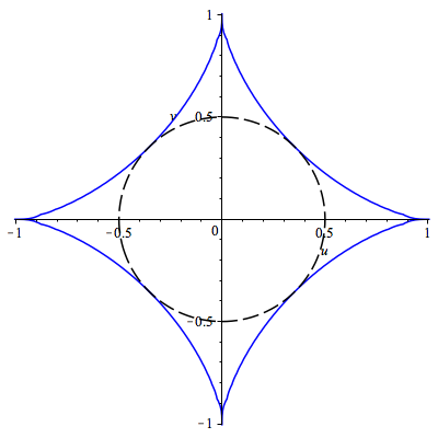
Figure 1: The space of parameters $(a,h)$.

Proposition 3.5.

We have that

• If $(a,h)$ is outside the astroid, then $P$ has $2$ roots and the index is $1/3$.

• If $(a,h)$ is inside the astroid, the $P$ has $4$ roots:

  • If $(a,h)$ is outside the dashed circle, then the index is $1/3$.

  • If $(a,h)$ is inside the dashed circle, then the index is $-1/3$.

It is proved in [3] that the phase portraits of a simple singularity is of type $D_{1}$, $D_{2}$ or $D_{3}$. It is clear that $D_{1}$ corresponds to points outside the astroid, $D_{2}$ to points inside the astroid but outside the circle, and $D_{3}$ to points inside the circle.

4 Semi-homogeneous elliptic cubic forms

4.1 Definition

Let $\omega$ be a cubic form and $p$ an isolated singularity of $\omega$. Denote by $\omega_{n}$ the order $n$-jet of $\omega$ at $p$. A cubic form is called semi-homogeneous (of degree $n$) if $\omega_{k}=0$, $k=1...,n-1$, and $\omega_{n}$ has $p$ as an isolated singularity (see [3]). Observe that for $n=1$ this definition reduces to the definition of a simple singularity.

The complex function $A+iB=C_{111}+iC_{222}$ can be approximated by $A_{n}+iB_{n}=C_{111}^{n}+iC_{222}^{n}$, where $C_{ijk}^{n}$ denotes the $n$-jet of $C_{ijk}$. More precisely

$$A+iB=A_{n}+iB_{n}+O_{n+1}(z,\bar{z}).$$

The semi-homogeneity assumption means that $A_{k}+iB_{k}=0$, $k=1,...,n-1,$ and $A_{n}+iB_{n}=0$ only for $z=\bar{z}=0$.

Lemma 4.1.

For a semi-homogeneous cubic form $\omega$ of degree $n$, the index of $\omega$ is given by

$$I=-\frac{\deg(A_{n}+iB_{n})}{3}.$$

Proof.

The same argument as in Lemma 3.1 shows that $\deg(A_{n}+iB_{n})=\deg(A+iB)$. Now the result follows from formula (3.6). ∎

4.2 Local model of a surface with semi-homogeneous cubic form

Assume that $f$ is given by equation (3.1). By a projective change of coordinates (see Lemma 3.4), we may assume $a_{22}=0$ and write

$$f(x,y)=\frac{1}{2}(x^{2}+y^{2})+\frac{1}{24}\left(a_{40}x^{4}+4a_{31}x^{3}y+4a_{13}xy^{3}+a_{04}y^{4}\right)+O_{5}(x,y).$$ (4.1)

Lemma 4.2.

Assume that $f$ is given by (4.1) and the $1$-jet of the cubic form is zero. Then

$$f(x,y)=\frac{1}{2}(x^{2}+y^{2})+O_{5}(x,y).$$ (4.2)

Proof.

From Appendix A.1 we have that

$$\omega_{1}=(ax+by)(dx^{3}-3dxdy^{2})+(cx+dy)(dy^{3}-3dydx^{2}),$$

where

$$a=a_{40},\ b=a_{31}-3a_{13},\ c=a_{13}-3a_{31}\ d=a_{04}.$$

Since, by hypothesis, $a=b=c=d=0$, we conclude that $a_{40}=a_{04}=a_{31}=a_{13}=0$. ∎

Lemma 4.3.

Assume that $f$ is given by (4.1) and the $(n-1)$-jet of the cubic form is zero. Then necessarily

$$f(x,y)=\frac{1}{2}(x^{2}+y^{2})+h(x,y)+O_{n+4}(x,y),$$ (4.3)

where $h=h_{n+3}$ is a homogeneous polynomial of degree $n+3$.

Proof.

Induction. The case $n=2$ was proved in Lemma 4.2. For $n\geq 3$, observe that the $(n-1)$-jet of the cubic form has $2n$ coefficients which are linear combinations of the $n+3$ coefficients of $h_{n+2}$, as proved in Appendix A.1. We have only to verify that this linear map is injective, which is straightforward. ∎

Lemma 4.3 says that if the cubic form is homogeneous of degree $n$, the surface is the graph of a function $f$ given by formula (4.3). Then Appendix A.1 says that

$$\omega_{n}=A_{n}(dx^{3}-3dxdy^{2})+B_{n}(dy^{3}-3dydx^{2}),$$

where

$$A_{n}+iB_{n}=h_{xxx}-3h_{xyy}+i(h_{yyy}-3h_{yxx}).$$ (4.4)

The semi-homogeneity hypothesis states that this function has $(0,0)$ as an isolated singularity.

4.3 Index of a semi-homogeneous cubic form

Theorem 4.4.

Consider an isolated singularity $p$ of the cubic form in the elliptic region of a surface. Assume that the cubic form at $p$ is semi-homogeneous. Then the index of the $3$-web is at most $1$.

Proof.

The index of $p$ coincides with the degree of $A_{n}+iB_{n}$ which is given by equation (4.4). Since

$$\frac{\partial^{3}h}{\partial{\bar{z}^{3}}}=h_{xxx}-3h_{xyy}-i(h_{yyy}-3h_{yxx})$$

Loewner’s conjecture ([14]) implies that the degree of $A_{n}+iB_{n}$ is $\geq-3$. Then Lemma 4.1 implies that the index of the $3$-web is at most $1$. ∎

A natural conjecture here is that the index of the cubic form is always $\leq 1$, even without the semi-homogeneity hypothesis.

5 Quadratic points in the hyperbolic region

Assume that $M$ is the graph of $f:U\subset\mathbb{R}^{2}\to\mathbb{R}$ given by

$$f(x,y)=xy+\frac{1}{24}\left(ax^{4}+4bx^{3}y+6ex^{2}y^{2}+4cxy^{3}+dy^{4}\right)+O_{5}(x,y).$$ (5.1)

Then the cubic form is given by

$$\omega=\omega_{1}+O_{2}(x,y),$$ (5.2)

where

$$\omega_{1}=(ax+by)dx^{3}+(cx+dy)dy^{3},$$ (5.3)

(see Appendix A.1). We say that the isolated singularity $(0,0)$ of $\omega$ is simple if it is also an isolated singularity of $\omega_{1}$, which is equivalent to

$$\delta=ad-bc\neq 0.$$ (5.4)

We observe that for a generic surface $M$, all quadratic points are simple.

5.1 Index of simple singularities

Denote by $X$ a vector field in the null direction of $\omega$. It follows from equation (5.2) that we can find a vector field $X_{1}$ in the null direction of $\omega_{1}$ such that

$$X-X_{1}=O_{2}(x,y).$$

Then the same argument as in the proof of Lemma 3.1 shows that the index of $X$ is equal to the index of $X_{1}$, which is equivalent to say that the indices of $\omega$ and $\omega_{1}$ coincide. Observe that the index of $\omega_{1}$ varies continuously with the parameters $(a,b,c,d)$ in the set $\delta\neq 0$, and thus it is constant in each connected component of this set.

Define the characteristic polynomial

$$P(x,y)=(ax+by)x^{3}+(cx+dy)y^{3}$$ (5.5)

and let

$$Q(x,y)=xy\left((ax+by)x-(cx+dy)y\right).$$ (5.6)

Lemma 5.1.

For simple singularities satisfying $ad\neq 0$, $P$ and $Q$ have no common roots.

Proof.

If $(x,y)$ is a root of $Q$ with $x\neq 0$ and $y\neq 0$, $(ax+by)x=(cx+dy)y$, and so

$$P(x,y)=(ax+by)x(x^{2}+y^{2}).$$

If $(x,y)$ is also a root of $P$, $ax+by=0$, which implies $cx+dy=0$, thus contradicting hypothesis (5.4). ∎

Lemma 5.2.

Denote $P(t)=P(\cos(t),\sin(t))$ and $Q(t)=Q(\cos(t),\sin(t))$. Up to a factor, we can write $\omega_{1}$ in polar coordinates as

$$\omega_{1}=P(t)dr^{3}-3rQ(t)dr^{2}dt+O_{2}(r)drdt^{2}+O_{3}(r)dt^{3},$$ (5.7)

where $O_{n}(r)$ denotes terms of order $\geq n$ in $r$.

Proof.

Straightforward calculations using $x=r\cos(t)$ and $y=r\sin(t)$. ∎

Lemma 5.3.

Assume $ad\neq 0$ and denote $\bar{X}_{1}$ the vector field

$$\bar{X}_{1}=(3xQ-yP)\frac{\partial}{\partial x}+(3yQ+xP)\frac{\partial}{\partial y}.$$

Then

$$||\bar{X}_{1}-X_{1}||=O_{2}(r).$$

Proof.

In polar coordinates,

$$\bar{X}_{1}=3rQ(t)\frac{\partial}{\partial r}+P(t)\frac{\partial}{\partial t}.$$

Using formula (5.7), we conclude the proof of the lemma. ∎

Proposition 5.4.

The index of the vector fields $X_{1}$ and $\bar{X}_{1}$ coincide.

Proof.

Similar to the proof of Lemma 3.1. ∎

Corollary 5.5.

Assume $ad\neq 0$. Then the index of a simple singularity is equal to the degree of the map $(x,y)\to(Q(x,y),P(x,y))$ plus $1$.

Proof.

By Proposition 5.4, the index of the simple singularity is given by the degree of the map $(x,y)\to(3xQ-yP,3yQ+xP)$. But the degree of this map is equal to the degree of the map $(x,y)\to(3Q,P)$ plus $1$. Finally the degree of $(3Q,P)$ is equal to the degree of $(Q,P)$. ∎

5.2 Polar blow-up of the linear form

We can write

$$\lambda_{1}=\cos(\phi)dx-\sin(\phi)dy,$$

where

$$\tan^{3}(\phi)=-\frac{cx+dy}{ax+by}.$$ (5.8)

Denote by $X_{1}$ a vector field in the kernel of $\lambda_{1}$.

Consider the polar projection $\pi:(-\delta,\delta)\times\mathbb{R}\to\mathbb{R}^{2}$ given by $\pi(r,t)=(r\cos(t),r\sin(t))$. Then straightforward calculations show that

$$\pi^{*}\lambda_{1}=\cos(\phi+t)dr-r\sin(\phi+t)dt.$$ (5.9)

Lemma 5.6.

Assume $ad\neq 0$. The singularities of $\pi^{*}\omega_{1}$ are of the form $(0,t_{0})$, where $t_{0}$ is a root of the characteristic polynomial $P$.

Proof.

We use Formula (5.7) with $\pi^{*}\omega_{1}$ in place of $\omega_{1}$. Thus, $\pi^{*}\omega_{1}(r,t)=0$ implies that $P(t)=0$. And since, by Lemma 5.1, $P$ and $Q$ have no common roots, we conclude that $r=0$. Conversely if $P(t)=0$ and $r=0$ is is obvious that $\pi^{*}(r,t)=0$. ∎

The vector field

$$\pi^{*}X_{1}=r\sin(\phi+t)\frac{\partial}{\partial r}+\cos(\phi+t)\frac{\partial}{\partial t}$$

is in the kernel of $\pi^{*}\lambda_{1}$. $\pi^{*}X_{1}$ is singular only at points $(0,t_{0})$ such that $\phi(t_{0})+t_{0}=k\pi+\frac{\pi}{2}$, $k\in\mathbb{Z}$. At these points

$$D(\pi^{*}X_{1})(0,t_{0})=(-1)^{k}\left[\begin{array}[]{cc}1&0\\ 0&-(1+\phi^{\prime}(t_{0}))\end{array}\right].$$

Observe that $(0,t_{0})$ is hyperbolic for $\pi^{*}X_{1}$ if and only if $1+\phi^{\prime}(t_{0})\neq 0$.

Lemma 5.7.

Assume $ad\neq 0$. Then, if $P(t_{0})=0$, we have that

$$P^{\prime}(t_{0})=-3Q(t_{0})(1+\phi^{\prime}(t_{0})).$$

Proof.

Differentiating equation (5.8) we obtain

$$-3\tan^{2}(\phi)\sec^{2}(\phi)\phi^{\prime}=\frac{ad-bc}{(a\cos t+b\sin t)^{2}}.$$

If $P(t)=0$, we have $\phi+t=\frac{\pi}{2}+k\pi$, and so $\sin(\phi)=\pm\cos(t)$, $\cos(\phi)=\pm\sin(t)$. Thus

$$3\phi^{\prime}=\frac{bc-ad}{(a\cos t+b\sin t)^{2}}\frac{\sin^{4}t}{\cos^{2}t}.$$

Moreover, since $P(t)=0$, $Q(t)=\frac{\cos^{2}t}{\sin t}(a\cos t+b\sin t)$. Thus

$$3Q\phi^{\prime}=\frac{bc-ad}{a\cos t+b\sin t}\sin^{3}t.$$

On the other hand,

$$P^{\prime}+3Q=(-a\sin t+b\cos t)\cos^{3}t+(-c\sin t+d\cos t)\sin^{3}t.$$

From $P(t)=0$ we obtain

$$P^{\prime}+3Q=\sin^{3}t\left((a\sin t-b\cos t)\frac{(c\cos t+d\sin t)}{a\cos t+b\sin t}+(-c\sin t+d\cos t)\right)$$

Thus $P^{\prime}+3Q=-3Q\phi^{\prime}$. ∎

Proposition 5.8.

Assume $ad\neq 0$. The singularity $(0,t_{0})$ of $\pi^{*}X_{1}$ is hyperbolic if and only if the root $t_{0}$ of $P$ is simple. Moreover, it is a saddle if and only if $P^{\prime}(t_{0})$ and $Q(t_{0})$ have opposite signs.

5.3 Parameter space in the hyperbolic region

We may write the characteristic polynomial as

$$P(x,y)=ax^{4}+bx^{3}y+cxy^{3}+dy^{4}.$$

This polynomial has multiple roots if and only if its discriminant $\Delta$ vanishes. In this case, we have that $\Delta=S^{3}-27T^{2}$, where

$$S=ad-\frac{bc}{4};\ \ T=-\frac{1}{16}(ac^{2}+db^{2}),$$

(see[11]). By section 5.2, the type of singularity is constant in the connected components of $\Delta=0$ and $ad=0$. On the other hand, by section 5.1, the index is constant in the connected components of $\delta=0$.

If $bc\neq 0$, by a projective change of coordinates, we may assume $b=\pm 4$, $c=\pm 4$ (see [13]), and we consider two different cases, $bc=16$ and $bc=-16$. The third case to consider is $bc=0$.

5.3.1 Case $bc=16$

For $bc=16$, we obtain

$$\Delta=(ad-4)^{3}-27(a+d)^{2};\ \ \delta=ad-16.$$

Proposition 5.9.

We have that

• If $\Delta>0$ (outside the full line in Figure 2), then $P$ has no roots and the index is $1$.

• If $\Delta<0$ (inside the full line in Figure 2), then $P$ has $2$ roots:

  • If $\delta>0$ (outside the dashed line in Figure 2), then the index is $1$.

  • If $\delta<0$ (inside the dashed line in Figure 2), then the singularity is a saddle and the index is $-1$.

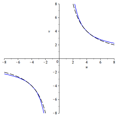
Figure 2: The space of parameters $(a,d)$ in case $bc=16$.

5.3.2 Case $bc=-16$

For $bc=-16$, we obtain

$$\Delta=(ad+4)^{3}-27(a+d)^{2};\ \ \delta=ad+16.$$

Proposition 5.10.

The full line curve in Figure 3 is $\Delta=0$. The region $\Delta>0$ is divided in a bounded region, that we shall call region $I$, and two unbounded regions, that we shall call region $II$. The region $\Delta<0$ is divided in two unbounded regions, that we shall call region $III$.

• If $(a,d)$ belongs to region $I$, then $P$ has $4$ roots and the index is $1$.

• If $(a,d)$ belongs to region $II$, then $P$ has no roots and the index is $1$.

• If $(a,d)$ belongs to region $III$, then $P$ has $2$ roots:

  • If $\delta>0$ (inside the dashed line in Figure 3), then the index is $1$.

  • If $\delta<0$ (outside the dashed line in Figure 3), then the singularity is a saddle and the index is $-1$.

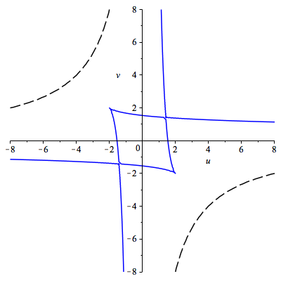
Figure 3: The space of parameters $(a,d)$ in case $bc=-16$.

5.3.3 Case $bc=0$

We shall assume without loss of generality that $b=0$ and $c=4$. In this case,

$$\Delta=a^{2}(ad^{3}-27);\ \delta=ad.$$

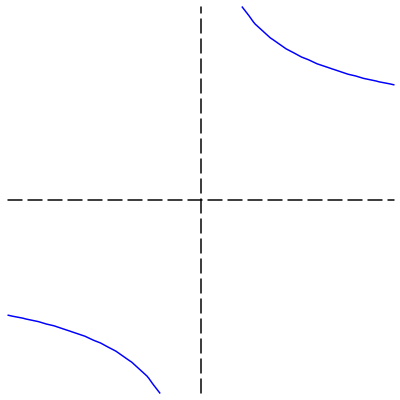
Figure 4: The space of parameters $(a,d)$ in case $bc=0$.

The full line in Figure 4 is $\Delta=0$, while the dashed lines are $\delta=0$.

Proposition 5.11.

We have that:

• If $(a,d)$ is in the second or fourth quadrants, then the index is $-1$.

• If $(a,d)$ is in the first or third quadrants, then the index is $+1$.

  • If $(a,d)$ is outside the full lines, then $P$ has no roots.

  • If $(a,d)$ is inside the full lines, then $P$ has $2$ roots.

5.4 Phase portraits of simple singularities

In this section we assume that the singularity is simple, $ad\neq 0$ and the characteristic polynomial $P$ has only simple roots. Under these hypothesis, we shall show that there are only four possible types of phase portraits, and they correspond to index $1$, $P$ with $0$, $2$ or $4$ roots and index $-1$, $P$ with $2$ roots.

We begin with some general facts: At consecutive roots of $P$, $\frac{dP}{dt}$ changes its sign. To find the sign of $Q$, observe that if $P=0$ then

$$(a\cos(t)+b\sin(t))\cos^{3}(t)=-(c\cos(t)+d\sin(t))\sin^{3}(t).$$

At such points

$$Q(t)=-\sin^{2}(t)\left(c+d\tan(t)\right).$$

So $Q(t)>0$, for $\tan(t)<-\frac{c}{d}$ and $Q(t)<0$, for $\tan(t)>-\frac{c}{d}$.

Case 1: $P$ has no real roots

In this case the index is $+1$.

Example 3.

Consider $a=1$, $b=2$, $c=-4$, $d=12$.

$$P=x^{4}+2x^{3}y-4xy^{3}+12y^{4}=(x^{2}-2xy+2y^{2})(x^{2}+4xy+6y^{2}).$$

The phase portrait of the line field can be seen in Figure 5.

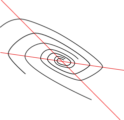
Figure 5: Line field of Example 3.

Case 2: $P$ has $4$ real roots

From the previous section, we may assume that $bc=-16$ and $(a,d)$ belongs to region $I$ (see Figure 3). It is also clear from our analysis that the type of the hyperbolic singularities of $\pi^{*}X_{1}$ are constant in each of the four regions $I1=\{(a,d)\in I|a>0,d>0\}$, $I2=\{(a,d)\in I|a<0,d>0\}$, $I3=\{(a,d)\in I|a<0,d<0\}$ and $I4=\{(a,d)\in I|a>0,d<0\}$. Thus to see the type of the hyperbolic singularities we must choose a pair $(a,d)$ in each of these four regions and compare $-\frac{c}{d}$ with the roots $s_{1}<s_{2}<s_{3}<s_{4}$ of $P$.

We have chosen the following pairs: For $(a,b,c,d)=(1,-4,4,1)\in I1$, we obtain $-\frac{c}{d}=-4<-1<s_{1}$. For $(a,b,c,d)=(-1,-4,4,-1)\in I3$, we obtain $-\frac{c}{d}=4>1>s_{4}$. For $(a,b,c,d)=(-\frac{8}{5},-4,4,\frac{8}{5})\in I2$, we obtain $-\frac{c}{d}=-\frac{5}{2}<s_{1}=-2$. For $(a,b,c,d)=(\frac{8}{5},-4,4,-\frac{8}{5})\in I4$, we obtain $-\frac{c}{d}=\frac{5}{2}>s_{4}=2$. We conclude that in any case, the sign of $Q$ at the roots of $P$ keep constant. Thus we have only parabolic sectors.

Example 4.

Consider

$$P(t)=\cos^{4}(t)(\tan(t)-s_{1})(\tan(t)-s_{2})(\tan(t)-s_{3})(\tan(t)-s_{4}),$$

where $s_{1}=-2$, $s_{2}=-1$, $s_{3}=1$ and $s_{4}=-\frac{1}{2}$. Then

$$a=-1,\ b=-\frac{5}{2},\ c=\frac{5}{2},\ d=1.$$

The phase portrait of the polar line field can be seen in Figure 6.

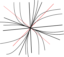
Figure 6: Line field of Example 4. Polar blowing-up resolution with eight hyperbolic singular points, four saddles and four nodes.

Case 3: $P$ has $2$ real roots

Assume that the roots of $P(t)$ are $t_{1}<t_{2}$. We write

$$P(t)=\cos^{2}(t)P_{2}(\cos t,\sin t)(\tan(t)-\tan(t_{1}))(\tan(t)-\tan(t_{2})),$$

for some quadratic polynomial $P_{2}(x,y)>0$. Then

$$P^{\prime}(t_{1})=P_{2}(\cos t_{1},\sin t_{1})(\tan(t_{1})-\tan(t_{2}))<0,$$

and similarly $P^{\prime}(t_{2})>0$. If the signs of $Q(t_{1})$ and $Q(t_{2})$ are the same, then there are only parabolic sectors, the singular point is a node and the index is $+1$. If $Q(t_{1})$ and $Q(t_{2})$ have different signs, then there are $4$ hyperbolic sectors, the singular point is a saddle and the index is $-1$.

Example 5.

Consider $P_{2}(x,y)=(y-x)^{2}+x^{2}$, $\tan(t_{1})=1$, $\tan(t_{2})=-\frac{4}{3}$. In other words, $a=-8/3$, $b=10/3$, $c=-5/3$, $d=1$. Then there are only parabolic sectors. The phase portrait of the line field can be seen in Figure 7.

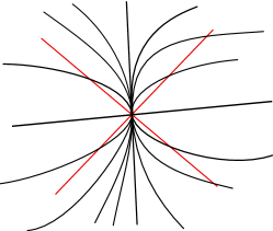
Figure 7: Line field of Example 5. Polar blowing-up resolution with four hyperbolic singular points, two saddles and two nodes.

Example 6.

Consider $a=-1$, $d=1$, $b=-1/2$, $c=1/2$. Then there are $2$ singular points of the blow-up, $\tan(t)=\pm 1$. There are $4$ hyperbolic sectors, thus the index is $-1$. The phase portrait of the line field can be seen in Figure 8.

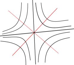
Figure 8: Line field of Example 6. Polar blowing up resolution with four hyperbolic singular points, all saddles.

6 Parabolic curve

Let $C$ be a parabolic curve of a surface $M$. Close to $C$ there are hyperbolic and elliptic regions $H$ and $E$. In this section we prove that generically, we can extend the line field $\mathcal{H}$ continuously to $C$ by considering the tangent lines $\mathcal{L}$ to $C$. We prove also that we can select a line field $\mathcal{E}_{1}$ of the $3$-web $\mathcal{E}$ of $E$ such that $\mathcal{E}_{1}$ can be continuously extended to $\mathcal{L}$.

Generically, a parabolic curve has fold points and a finite number of Gauss points, also called godrons ([6]).

6.1 The cubic form in a neighborhood of a fold point

A generic surface $M$ at a fold point is given by

$$z=\frac{1}{2}x^{2}+\frac{1}{6}y^{3}.$$ (6.1)

(see [6]).

Proposition 6.1.

Assume that $M$ is given by equation (6.1). Then the cubic form is conformally equivalent to $-3dx^{2}dy+ydy^{3}$.

Proof.

See Appendix A.2. ∎

From the above proposition we conclude that, at a fold point, there exists a line field $\mathcal{L}$ that coincides with $\mathcal{H}$ in the hyperbolic part, with a line field $\mathcal{E}_{1}$ of the $3$-web $\mathcal{E}$ in the elliptic part at is tangent to the parabolic curve.

6.2 The cubic form in a neighborhood of a Gauss cusp

A generic surface in a neighborhood of a Gauss cusp is given by

$$z=\frac{1}{2}x^{2}+\frac{1}{2}xy^{2}+\frac{\lambda}{24}y^{4},$$ (6.2)

for some $\lambda\neq 0,3$ (see [9] and also [15]).

Proposition 6.2.

Assume that $M$ is given by equation (6.2). Then the cubic form is conformally equivalent to

$$C_{111}=-3,\ C_{112}=-\lambda y,\ C_{122}=3x-\lambda\frac{y^{2}}{2},$$

$$C_{222}=y\left(x(6+\lambda)+\lambda(\lambda-2)\frac{y^{2}}{2}\right).$$

Proof.

See Appendix A.2. ∎

From the above proposition we conclude that, at a Gauss cusp, there exists a line field $\mathcal{L}$ that coincides with $\mathcal{H}$ in the hyperbolic part, with a line field $\mathcal{E}_{1}$ of the $3$-web $\mathcal{E}$ in the elliptic part at is tangent to the parabolic curve.

7 Poincaré-Hopf type theorems

7.1 Elliptic region

Consider now an elliptic region $E$ bounded by a parabolic curve $C$. Let $\mathcal{E}$ denote the $3$-web of the cubic form in the region $E$. As we have seen above, in a neighborhood of $C$ one of the line field $\mathcal{E}_{1}$ of the $3$-web $\mathcal{E}$ can be continuously extended to $C$ by considering $\mathcal{E}_{1}$ tangent to $C$.

Proposition 7.1.

We have that

$$\sum_{p_{i}\in E}Ind(p_{i},\mathcal{E})=\chi(E).$$

where the sum is taken over the quadratic points $p_{i}$.

Proof.

In this proof we follow [1] and [3]. Assume first that $M$ is orientable, for non-orientable surfaces consider a double covering. Fix an orientation and a Riemannian metric on $M$.

Take a triangulation $\mathcal{T}$ such that each triangle $T\in\mathcal{T}$ contains at most one singular point $p_{T}$ in its interior. Take $X$ any vector field in the kernel of $\omega$. Then

$$\int_{T}Kd\sigma-2\pi Ind(\omega,p_{T})=\frac{1}{6}\int_{6\partial T}\left[\frac{DX}{ds}\right]ds,$$

where $\left[\frac{DX}{ds}\right]$ denotes the algebraic value of the covariant derivative and the notation $6\partial{T}$ means $6$ times the boundary of $T$. Summing we obtain

$$\int_{E}Kd\sigma-2\pi\sum_{p\in E}Ind(\omega,p)=\int_{C}\left[\frac{DX}{ds}\right]ds=-\int_{C}k_{g}ds,$$

where the last equality comes from the fact that we can choose $X$ tangent to $C$. Now the Gauss-Bonnet theorem implies that

$$\sum_{p\in E}Ind(\omega,p)=\chi(E),$$

thus proving the proposition. ∎

Corollary 7.2.

A generic compact convex surface $M$ in $\mathbb{P}^{3}$ has at least $6$ quadratic points.

Corollary 7.3.

Let $M$ be a compact convex surface in $\mathbb{P}^{3}$ and assume that the cubic forms at the quadratic points are semi-homogeneous. Then $M$ has at least $2$ quadratic points.

Corollary 7.3 is a version of Carathédory conjecture for quadratic points, assuming that the cubic forms are semi-homogeneous. One can conjecture that Corollary 7.3 remains valid without this assumption.

7.2 A compact convex surface with two quadratic points

Consider a smooth rotation surface $S$ with axis $L$. The points of $L\cap S$ are quadratic of index $1$.

We describe below a compact rotation surface $S$ with $2$ points of intersection with the axis $L$ and no other quadratic point. In rectangular coordinates $(x_{1},x_{2},y)$, the equation of $S$ is

$$x_{1}^{2}+x_{2}^{2}+y^{2}(1+\lambda y)^{2}=(1+\lambda y)^{2},$$

for some constant $\lambda>0$ small.

Let $(x(s),y(s))$ be a curve satisfying

$$x^{\prime}y^{\prime\prime}-y^{\prime}x^{\prime\prime}=1$$ (7.1)

and consider the rotation surface

$$\psi(s,\theta)=\left(x(s)\cos\theta,x(s)\sin\theta,y(s)\right).$$ (7.2)

Proposition 7.4.

Assume $M$ is given by equation (7.2). Then the quadratic points are given by the equation $xy^{\prime\prime}=x^{\prime}y^{\prime}$.

Proof.

See Appendix B. ∎

Example 7.

Take

$$(x(t),y(t))=\left(\cos(t)(1+\lambda\sin(t)),\sin(t)\right),\ \ -\frac{\pi}{2}\leq t\leq\frac{\pi}{2},$$

for some constant $\lambda>0$ small (see Figure 9).

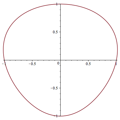
Figure 9: A section of the rotation surface ($\lambda=0.2$).

Then

$$\Delta=x_{t}y_{tt}-x_{tt}y_{t}=1+3\lambda\sin t-2\lambda\sin^{3}t.$$

Observe that $y^{\prime}=y_{t}\frac{dt}{ds}=\cos(t)\Delta^{-1/3}$ and so

$$\frac{y^{\prime}}{x}=\frac{\Delta^{-1/3}}{1+\lambda\sin t}.$$

Then

$$\left(\frac{y^{\prime}}{x}\right)_{t}=-\frac{\Delta^{-4/3}}{3(1+\lambda\sin t)^{2}}\left(\Delta_{t}(1+\lambda\sin t)+3\Delta\lambda\cos t\right)$$

Since

$$\Delta_{t}(1+\lambda\sin t)+3\lambda\cos t\Delta=6\lambda\cos^{3}t(1+2\lambda\sin t),$$

we conclude that $\left(\frac{y^{\prime}}{x}\right)_{t}<0$, or equivalently $\left(\frac{y^{\prime}}{x}\right)^{\prime}<0$. This implies that there no quadratic points other than $(0,0,\pm 1)$.

7.3 Hyperbolic region

Consider an hyperbolic region $H$ bounded by a parabolic curve $C$. Let $\mathcal{H}$ be the line field of the cubic form in the region $H$. As we have seen above, generically $\mathcal{H}$ can be extended continuously to $C$ by considering $\mathcal{H}$ tangent to $C$. Thus the classical Poincaré-Hopf Theorem implies the following:

Proposition 7.5.

Let $H$ be the hyperbolic region of a generic surface $M$. Then

$$\sum_{p_{i}\in H}Ind(p_{i},\mathcal{H})=\chi(H),$$

where the sum is taken over the quadratic points $p_{i}$.

The following corollary is proved in [15]:

Corollary 7.6.

A generic hyperbolic disc has an odd number of quadratic points.

7.4 A general result

The following general result is a consequence of Propositions 7.1 and 7.5:

Theorem 7.7.

Denote by $E$ and $H$ the elliptic and hyperbolic regions of a generic compact surface $M$ in the projective space $\mathbb{P}^{3}$. Then

$$\sum_{p_{i}\in E}Ind(p_{i},\mathcal{E})+\sum_{p_{i}\in H}Ind(p_{i},\mathcal{H})=\chi(M),$$

where the sum is taken over the quadratic points $p_{i}$.

Appendix A Cubic form of graphs of functions

A.1 Elliptic and hyperbolic quadratic points

Assume

$$\psi(x,y)=(x,y,f(x,y))$$

and write $\phi^{4}=f_{xx}f_{yy}-f_{xy}^{2}$. Then the Blaschke metric is given by

$$g_{11}=\frac{f_{xx}}{\phi};\ g_{11}=\frac{f_{xy}}{\phi};\ g_{22}=\frac{f_{yy}}{\phi}.$$

The affine normal $\xi$ is given by

$$\xi=\phi(0,0,1)+Z_{1}\psi_{x}+Z_{2}\psi_{y},$$

where

$$\begin{array}[]{l}Z_{1}=\frac{1}{\phi^{4}}\left(-f_{yy}\phi_{x}+f_{xy}\phi_{y}\right)\cr Z_{2}=\frac{1}{\phi^{4}}\left(f_{xy}\phi_{x}-f_{xx}\phi_{y}\right)\end{array}$$

(see [8, p.47]). Writing

$$\psi_{xx}=\Gamma_{11}^{1}\psi_{x}+\Gamma_{11}^{2}\psi_{y}+g_{11}\xi$$

and using the above formulas we obtain

$$\begin{array}[]{l}\Gamma_{11}^{1}+g_{11}Z_{1}=0\cr\Gamma_{11}^{2}+g_{11}Z_{2}=0.\end{array}$$

Thus

$$C_{111}=(g_{11})_{x}-2\left(\Gamma_{11}^{1}g_{11}+\Gamma_{11}^{2}g_{12}\right)=(g_{11})_{x}+2\left(g_{11}^{2}Z_{1}+g_{11}g_{12}Z_{2}\right).$$

Straightforward calculations show that

$$C_{111}=\frac{1}{\phi^{5}}\left(-3f_{xx}\phi^{3}\phi_{x}+f_{xxx}\phi^{4}\right)$$

and so,

$$\phi^{5}C_{111}=\frac{1}{4}f_{xxx}f_{xx}f_{yy}-\frac{3}{4}f_{xyy}f_{xx}^{2}+\frac{3}{2}f_{xxy}f_{xx}f_{xy}-f_{xxx}f_{xy}^{2}.$$ (A.1)

Similarly we obtain

$$\phi^{5}C_{112}=-\frac{1}{4}f_{xx}^{2}f_{yyy}+\frac{3}{4}f_{xx}f_{yy}f_{xxy}-\frac{1}{2}f_{xy}f_{yy}f_{xxx}.$$ (A.2)

$$\phi^{5}C_{122}=-\frac{1}{4}f_{yy}^{2}f_{xxx}+\frac{3}{4}f_{xx}f_{yy}f_{xyy}-\frac{1}{2}f_{xy}f_{xx}f_{yyy}.$$ (A.3)

$$\phi^{5}C_{222}=\frac{1}{4}f_{yyy}f_{xx}f_{yy}-\frac{3}{4}f_{xxy}f_{yy}^{2}+\frac{3}{2}f_{xyy}f_{yy}f_{xy}-f_{yyy}f_{xy}^{2}.$$ (A.4)

Lemma A.1.

Assume

$$f(x,y)=\frac{1}{2}(x^{2}+y^{2})+h(x,y),$$

where $h=h_{n+3}$ is a non-zero homogeneous polynomial of degree $n+3$. Then, up to common factor, the cubic form of $f$ is given by

$$\omega=C_{111}(dx^{3}-3dxdy^{2})+C_{222}(dy^{3}-3dydx^{2}),$$

where

$$\left\{\begin{array}[]{l}C_{111}=h_{xxx}-3h_{xyy}+O(n+1)\cr C_{222}=h_{yyy}-3h_{yxx}+O(n+1).\end{array}\right.$$

Proof.

Taking the parcels of order at most $n$ in formulas (A.1), (A.2), (A.3) and (A.4), we prove the result. ∎

Lemma A.2.

Assume $f$ is given by equation (5.1). Then the cubic form is given by equation (5.3).

Proof.

Take the parcels of order at most $1$ in formulas (A.1), (A.2), (A.3) and (A.4). ∎

A.2 Cubic forms at parabolic points

Proof of Proposition 6.1

Assume $M$ is given by (6.1). Then

$$X=(1,0,f_{x})=(1,0,x),\ \ Y=(0,1,f_{y})=(0,1,\frac{y^{2}}{2}),$$

$L=1,N=y,M=0$, $LN-M^{2}=y$, and so $(x,y)$ is parabolic if $y=0$, elliptic if $y>0$ and hyperbolic if $y<0$. Let $\phi=|y|^{1/4}$. Then

$$g(X,X)=\frac{1}{\phi},\ g(X,Y)=0,\ g(Y,Y)=\frac{y}{\phi}.$$

The affine normal is $\xi=\phi\xi_{0}+Z_{1}X+Z_{2}Y$, $\xi_{0}=(0,0,1)$, where $Z_{1}=-\phi_{x}=0$, $Z_{2}=-\frac{\phi_{y}}{y}=\mp\frac{1}{4y\phi^{3}}$. Moreover

$$\nabla_{X}X=\pm\frac{1}{4y\phi^{4}}Y,\ \ \nabla_{X}Y=0,\ \ \nabla_{Y}Y=\pm\frac{1}{4\phi^{4}}Y.$$

Thus $C(X,X,X)=C(X,Y,Y)=0$, $C(X,X,Y)=\mp\frac{1}{4\phi^{5}}$ and

$$C(Y,Y,Y)=\mp\frac{y}{4\phi^{5}}+\frac{1}{\phi}\mp 2\frac{y}{4\phi^{5}}=\pm\frac{1}{4\phi^{5}}y,$$

which proves Proposition 6.1.

Proof of Proposition 6.2

Assume $M$ is given by equation (6.2). Then

$$X=(1,0,f_{x})=(1,0,x+\frac{1}{2}y^{2}),\ \ Y=(0,1,f_{y})=(0,1,xy+\lambda\frac{y^{3}}{6}),$$

$$f_{xx}=(0,0,1),\ \ f_{xy}=(0,0,y),\ \ f_{yy}=(0,0,x+\lambda\frac{y^{2}}{2}),\ \ \phi^{4}=\left|x+(\lambda-2)\frac{y^{2}}{2}\right|,$$

and the Blaschke metric is given by

$$g(X,X)=\frac{1}{\phi},\ g(X,Y)=\frac{y}{\phi},\ g(Y,Y)=\frac{x+\lambda\frac{y^{2}}{2}}{\phi}.$$

We can write $\xi=\phi\xi_{0}+Z_{1}X+Z_{2}Y,\ \ \xi_{0}=(0,0,1)$, where

$$Z_{1}+yZ_{2}=-\phi_{x},\ \ yZ_{1}+(x+\lambda\frac{y^{2}}{2})Z_{2}=-\phi_{y}.$$

Elliptic points

Assume $x+(\lambda-2)\frac{y^{2}}{2}>0$. Then

$$\phi_{x}=\frac{1}{4\phi^{3}},\ \ \phi_{y}=\frac{1}{4\phi^{3}}(\lambda-2)y,$$

and so

$$(Z_{1},Z_{2})=\frac{1}{4\phi^{7}}\left(-x+(\lambda-4)\frac{y^{2}}{2},(3-\lambda)y\right).$$

Then

$$\nabla_{X}X=-\frac{f_{xx}}{\phi}(Z_{1}X+Z_{2}Y)=\frac{1}{4\phi^{8}}\left[\left(x-(\lambda-4)\frac{y^{2}}{2}\right)X+(\lambda-3)yY\right],$$

$$\nabla_{X}Y=y\nabla_{X}X,\ \ \nabla_{Y}Y=\left(x+\lambda\frac{y^{2}}{2}\right)\nabla_{X}X.$$

The cubic form is thus

$$C_{111}=-\frac{1}{4\phi^{5}}-\frac{2}{4\phi^{9}}\left[\left(x-(\lambda-4)\frac{y^{2}}{2}\right)+(\lambda-3)y^{2}\right]=-\frac{3}{4\phi^{5}}.$$

$$C_{112}=\frac{(2-\lambda)y}{4\phi^{5}}-\frac{2y}{4\phi^{9}}\left[\left(x-(\lambda-4)\frac{y^{2}}{2}\right)+(\lambda-3)y^{2}\right]=-\frac{\lambda y}{4\phi^{5}}.$$

$$C_{122}=\frac{1}{\phi}-\frac{1}{4\phi^{5}}(x+\lambda\frac{y^{2}}{2})-2yg(\nabla_{X}X,Y)=\frac{1}{4\phi^{5}}(3x-\lambda\frac{y^{2}}{2}).$$

$$C_{222}=\frac{\lambda y}{\phi}-\frac{(\lambda-2)y}{4\phi^{5}}(x+\lambda\frac{y^{2}}{2})-2(x+\lambda\frac{y^{2}}{2})g(\nabla_{X}X,Y)$$

$$C_{222}=\frac{y}{4\phi^{5}}(x(6+\lambda)+\lambda(\lambda-2)\frac{y^{2}}{2}).$$

Hyperbolic points

Assume $x+(\lambda-2)\frac{y^{2}}{2}<0$. Then $\phi^{4}=-x+(2-\lambda)\frac{y^{2}}{2}$,

$$\phi_{x}=-\frac{1}{4\phi^{3}},\ \ \phi_{y}=\frac{1}{4\phi^{3}}(2-\lambda)y.$$

The formulas for $Z_{1}$, $Z_{2}$, $\nabla_{X}X$, $\nabla_{X}Y$, $\nabla_{Y}Y$ remain the same. The formulas for $C_{ijk}$ also remain the same.

Appendix B Cubic form of a rotation surface

In this appendix we prove Proposition 7.4. Assume $M$ is a rotation surface given by equation (7.2). Then

$$\left\{\begin{array}[]{l}\psi_{s}=\left(x^{\prime}\cos\theta,x^{\prime}\sin\theta,y^{\prime}\right)\cr\psi_{\theta}=\left(-x\sin\theta,x\cos\theta,0\right)\end{array}\right.$$

Thus

$$\psi_{s}\times\psi_{\theta}=x\left(-y^{\prime}\cos\theta,-y^{\prime}\sin\theta,x^{\prime}\right).$$

Moreover,

$$\left\{\begin{array}[]{l}\psi_{ss}=\left(x^{\prime\prime}\cos\theta,x^{\prime\prime}\sin\theta,y^{\prime\prime}\right)\cr\psi_{s\theta}=\left(-x^{\prime}\sin\theta,x^{\prime}\cos\theta,0\right)\cr\psi_{\theta\theta}=-\left(x\cos\theta,x\sin\theta,0\right)\end{array}\right.$$

Thus

$$L=x;\ \ M=0;\ \ N=x^{2}y^{\prime};\ \ \phi^{4}=x^{3}y^{\prime}.$$

Then

$$\nu=\frac{x}{\phi}\left(-y^{\prime}\cos\theta,-y^{\prime}\sin\theta,x^{\prime}\right),\ \ g_{11}=\frac{x}{\phi};\ \ g_{12}=0;\ \ g_{22}=\frac{x^{2}y^{\prime}}{\phi}.$$

Lemma B.1.

The affine normal vector field $\xi$ can be written as

$$\xi=\left(a\cos\theta,a\sin\theta,b\right),$$

for certain $a=a(s)$, $b=b(s)$.

Proof.

Observe that $\nu_{\theta}\cdot\xi=0$. The conditions $\nu\cdot\xi=1$ and $\nu_{s}\cdot\xi=0$ are given by

$$\left\{\begin{array}[]{l}-ay^{\prime}+bx^{\prime}=\frac{\phi}{x}\cr-ay^{\prime\prime}+bx^{\prime\prime}=-\left(\frac{\phi}{x}\right)^{2}\left(\frac{x}{\phi}\right)^{\prime}\end{array}\right.$$

This system certainly has a solution $(a,b)$. ∎

We can write

$$\left\{\begin{array}[]{l}\psi_{ss}=\alpha\psi_{s}+h_{11}\xi\cr\psi_{s\theta}=\frac{x^{\prime}}{x}\psi_{\theta}\cr\psi_{\theta\theta}=\beta\psi_{s}+h_{22}\xi\end{array}\right.$$

Thus

$$\nabla_{\psi_{s}}\psi_{s}=\alpha\psi_{s};\ \ \nabla_{\psi_{s}}\psi_{\theta}=\nabla_{\psi_{\theta}}\psi_{s}=\frac{x^{\prime}}{x}\psi_{\theta};\ \ \nabla_{\psi_{\theta}}\psi_{\theta}=\beta\psi_{s}.$$

Then

$$C(\psi_{\theta},\psi_{\theta},\psi_{\theta})=-2g(\nabla_{\psi_{\theta}}\psi_{\theta},\psi_{\theta})=0;\ \ C(\psi_{s},\psi_{s},\psi_{\theta})=-2g(\nabla_{\psi_{\theta}}\psi_{s},\psi_{s})=0,$$

$$C(\psi_{s},\psi_{\theta},\psi_{\theta})=(g_{22})_{s}-2g(\nabla_{\psi_{s}}\psi_{\theta},\psi_{\theta})=\left(\frac{x^{2}y^{\prime}}{\phi}\right)^{\prime}-2\frac{x^{\prime}}{x}\frac{x^{2}y^{\prime}}{\phi}.$$

By the apolarity condition, a point is quadratic if and only if $C(\psi_{s},\psi_{\theta},\psi_{\theta})=0$. This condition is equivalent to

$$\frac{1}{\phi^{2}}\left((2xx^{\prime}y^{\prime}+x^{2}y^{\prime\prime})\phi-\phi^{\prime}x^{2}y^{\prime}\right)=2\frac{xx^{\prime}y^{\prime}}{\phi}.$$

After some simplifications we obtain that this condition is equivalent to
$xy^{\prime\prime}-x^{\prime}y^{\prime}=0$, thus proving Proposition 7.4.

References

- [1] M.P.do Carmo: Differential geometry of curves and surfaces, Prentice-hall, Inc., Englewood Cliffs, N.J., 1976.
- [2] B.Freitas and R.Garcia: Inflection points on hyperbolic tori of , pre-print, 2017.
- [3] T.Fukui and J.J.Nuño-Ballesteros: Isolated singularities of binary differential equations of degree n, Publ.Mat, 56, 65-89, 2012.
- [4] G.Darboux: Sur le contact des courbes et des surfaces, Bull.Sci.Math.Ast., serie 2, tome 4(1), 348-384, 1880.
- [5] V.V.Ivanov: The analytic Carathéodory conjecture, Siberian Math.J. 43(2), 251-322, 2002.
- [6] S.Izumiya, M.C.R.Fuster, M.A.S.Ruas and F.Tari: Differential Geometry from a Singularity Theory Viewpoint, World Scientific, 2015.
- [7] E.P.Lane: A treatise on projective differential geometry, The University of Chicago Press, 1942.
- [8] K.Nomizu and T.Sasaki: Affine differential geometry, Cambridge University Press, 1994.
- [9] O.A.Platonova:Singularities of relative position of a surface and a line, Russian Math.Surveys, 36(1), 248-249, 1981.
- [10] I.R.Porteous: Geometric Differentiation for the Intelligence of Curves and Surfaces, Cambridge University Press, 1994.
- [11] T.Poston and I.Stewart: The cross-ratio foliation of binary quartic forms, Geom. Dedicata, 27, 263-280, 1988.
- [12] V.Ovsienko and S.Tabachnikov: Projective Differential Geometry Old and New, Cambridge University Press, 2005.
- [13] V.Ovsienko and S.Tabachnikov: Hyperbolic Carathéodory conjecture, Proc. Steklov Inst.Math. 258, 178-193, 2007.
- [14] C.J.Titus:A proof of a conjecture of Loewner and of the conjecture of Carathéodory on umbilic points, Acta Math, 131(1-2), 43-77, 1973.
- [15] R. Uribe-Vargas:A projective invariant for swallowtails and godrons, and global theorems on the flecnodal curve, Moscow Math.J. 6(4), 731-768, 2006.