Performance Analysis of Massive MIMO with Low-Resolution ADCs

Abstract

The uplink performance of massive multiple-input-multiple-output (MIMO) systems where the base stations (BS) employ low-resolution analog-to-digital converters (ADCs) is analyzed. A high performance MMSE receiver that takes both additive white Gaussian noise (AWGN) and quantization noise into consideration is designed, which works well for both cases of uniform resolution ADCs and non-uniform resolution ADCs. With the proposed MMSE receiver, we then employ the random matrix theory to derive the asymptotic equivalent of the uplink spectral efficiency (SE) of the system. Numerical results show the tightness of the asymptotic equivalent of the uplink SE, and massive MIMO with low-resolution ADCs can still achieve the satisfying uplink SE by increasing the number of antennas at BS.

I Introduction

Massive multiple-input multiple-output (MIMO) has been considered as one of the key enabling technologies for 5G wireless communications systems, and thus has recently drawn lots of research interest. It could bring significant spectral efficiency (SE) and energy efficiency (EE) gains when the base station (BS) has a large number of antennas [1], [2]. Due to the large number of antennas at BS, a simple linear receiver can be employed to achieve a high SE, and the impact of imperfect hardware can also be mitigated. Most of the current works concerning massive MIMO systems assume each antenna at BS is equipped with a high-resolution ADC. However, high-resolution ADCs can incur substantial power assumption and high-cost hardware implementation [3], which may be not affordable in practical massive MIMO systems. This motives us to study the use of low-resolution ADCs to understand their impact on the performance of the system.

Several recent works have investigated the effects of low-resolution ADCs on the performance of massive MIMO systems [4]-[6]. In these works, the effect of low-resolution ADCs is described by using the additive quantization noise model (AQNM) [4]. Using AQNM, Fan et al. [5] derive an approximate analytical expression for the uplink achievable rate of massive MIMO systems over Rayleigh fading channels when low-resolution ADCs and the maximal-ratio combining (MRC) technique are used at the receiver; Zhang et al. [6] derive tractable and exact approximation expressions for the uplink SE of massive MIMO systems with low-resolution ADCs and MRC over Rician fading channels, where both perfect and imperfect channel state information (CSI) are considered. However, only uniform resolution ADCs and MRC receiver are considered in [5] and [6], which cannot be applied to analyze the uplink SE performance of massive MIMO systems with non-uniform resolution ADCs and MMSE receiver. In [7], a mixed-ADC architecture for massive MIMO systems is proposed, in which the BS antennas are equipped with both high-resolution ADCs and low-resolution ADCs. Under mixed-ADC massive MIMO with MRC receiver, the closed-form approximate expressions for the uplink achievable rate are derived for both perfect and imperfect CSI when the Rician fading channels are considered [8]. In [9], the asymptotic equivalent of the uplink SE is obtained when non-uniform resolution ADCs and MMSE receivers are used at the BS of massive MIMO systems. The MMSE receiver designed in [9] could cause significant SE loss for massive MIMO systems with non-uniform resolution ADCs. This is because it does not consider non-uniform quantization noise incurred by non-uniform resolution ADCs.

In this letter, with AQNM, we first design a proper MMSE receiver for the uplink massive MIMO system with low-resolution ADCs. The proposed MMSE receiver takes both additive white Gaussian noise (AWGN) and quantization noise into account. It can work well for both cases of uniform resolution ADCs and non-uniform resolution ADCs. We then derive a tight asymptotic equivalent of the uplink SE using random matrix theory. Finally, numerical results are obtained to verify our theoretical analysis.

Notations: Boldface lower and upper-case symbols represent vectors and matrices, respectively. The ${N\times N}$ identity matrix reads as ${{\bf{I}}_{N}}$. let ${{\bf{X}}^{H}}$ and ${\mathop{\rm tr}\nolimits}\left({\bf{X}}\right)$ be the conjugate transpose and trace of a matrix ${\bf{X}}$. ${\mathop{\rm diag}\nolimits}\left({\bf{X}}\right)$ keeps only the diagonal entries of ${\bf{X}}$. A random vector ${\bf{x}}\sim{\cal C}{\cal N}\left({{\bf{m}},{\bf{V}}}\right)$ is complex Gaussian distributed with mean vector ${\bf{m}}$ and covariance matrix ${\bf{V}}$. $\overset{a.s.}{\longrightarrow}$ denotes almost sure convergence.

II System Model

Consider an uplink massive MIMO system with low-resolution ADCs, where the BS equipped with $M$ antennas receives signal from $K$ single-antenna users using the same time-frequency resources. The received signal ${\bf{y}}\in{{\mathbb{C}}^{M\times 1}}$ at BS can be written as

$${\bf{y}}=\sqrt{{p_{u}}}{\bf{Gx}}+{\bf{n}},$$ (1)

where ${p_{u}}$ is the average transmit power of each user, ${\bf{x}}\in{{\mathbb{C}}^{K\times 1}}$ is the transmit vector for all $K$ users, and ${\bf{n}}\sim{\cal C}{\cal N}\left({0,{{\bf{I}}_{M}}}\right)$ is the normalized AWGN vector. The input covariance matrix ${{\bf{R}}_{\bf{x}}}={{\bf{I}}_{K}}$ is assumed. The channel matrix ${\bf{G}}\in{{\mathbb{C}}^{M\times K}}$ between the BS and all users is given as

$${\bf{G}}={\bf{H}}{{\bf{D}}^{{1\mathord{\left/{\vphantom{12}}\right.\kern-1.2pt}2}}},$$ (2)

where $\bf{H}$ denotes the small-scale fading channel matrix and ${\bf{D}}$ is the $K\times K$ diagonal matrix with diagonal entries $\left\{{{\beta_{k}}}\right\}$ to model the large-scale fading. Rayleigh fading is assumed here, thus without loss of generality, the elements of ${\bf{H}}$ can be considered to follow distribution ${\cal C}{\cal N}\left({0,1}\right)$.

As the quantization error can be well approximated as a linear gain with AQNM [4], the output vector of low-resolution ADCs can be expressed as

$${{\bf{y}}_{q}}={\bf{Q}}\left({\bf{y}}\right)\approx\Lambda{\bf{y}}+{{\bf{n}}_{q}}=\sqrt{{p_{u}}}\Lambda{\bf{Gx}}+\Lambda{\bf{n}}+{{\bf{n}}_{q}},$$ (3)

where ${\bf{Q}}\left(\cdot\right)$ is the quantizer function which applies component-wise and separately to the real and imaginary parts, and ${{\bf{n}}_{q}}$ is the additive Gaussian quantization noise vector which is uncorrelated with ${\bf{y}}$. The linear gain matrix $\Lambda$ is an $M\times M$ diagonal matrix with entries $\left\{{{\alpha_{m}}}\right\}$, and the linear gain coefficient ${\alpha_{m}}=1-{\rho_{m}}$, where ${\rho_{m}}$ is the inverse of the signal-to-quantization-noise ratio. Given a fixed channel realization ${\bf{G}}$, the covariance matrix of ${{\bf{n}}_{q}}$ can be written as [5]

$$\begin{array}[]{l}{{\bf{R}}_{{{\bf{n}}_{q}}}}={\rm E}\left({{{\bf{n}}_{q}}{\bf{n}}_{q}^{H}\left|{\bf{G}}\right.}\right)\\ {\rm{~{}~{}~{}~{}~{}=}}\Lambda\left({{{\bf{I}}_{M}}-\Lambda}\right){\bf{diag}}\left({{p_{u}}{\bf{G}}{{\bf{G}}^{H}}+{{\bf{I}}_{M}}}\right).\end{array}$$ (6)

III Asymptotic Equivalent of the Uplink Spectral Efficiency

In this section, using random matrix theory, we derive the asymptotic equivalent of the uplink SE for massive MIMO systems with low-resolution ADCs, when the MMSE receiver is considered. Here the perfect CSI is known at the BS. First, the proposed high-performance MMSE receiver is designed as

$${\bf{W}}={{\bf{G}}^{H}}{\Lambda^{H}}{\left({\Lambda{\bf{G}}{{\bf{G}}^{H}}{\Lambda^{H}}+{\bf{Z}}+\theta{{\bf{I}}_{M}}}\right)^{-1}},$$ (7)

where ${\bf{Z}}=\frac{1}{{{p_{u}}}}{{\bf{\bar{R}}}_{{{\bf{n}}_{q}}}}=\frac{1}{{{p_{u}}}}\Lambda\left({{{\bf{I}}_{M}}-\Lambda}\right)\left({{p_{u}}{\bf{tr}}\left({\bf{D}}\right)+1}\right)$, and $\theta={1\mathord{\left/{\vphantom{1{{p_{u}}}}}\right.\kern-1.2pt}{{p_{u}}}}$. ${{\bf{\bar{R}}}_{{{\bf{n}}_{q}}}}$ is the expectation of ${{\bf{R}}_{{{\bf{n}}_{q}}}}$ with respect to ${\bf{G}}$. Thus, we can see that the proposed MMSE receiver can suppress both AWGN and quantization noise at the same time. This proposed MMSE receiver will be used in the following analysis. By multiplying ${\bf{W}}$ with ${{\bf{y}}_{q}}$, the quantized output vector is processed as

$${\bf{r}}={\bf{W}}{{\bf{y}}_{q}}=\sqrt{{p_{u}}}{\bf{W}}\Lambda{\bf{Gx}}+{\bf{W}}\Lambda{\bf{n}}+{\bf{W}}{{\bf{n}}_{q}}.$$ (8)

The output signal for the $k{\rm{th}}$ user can be expressed as

$$\begin{array}[]{l}{{\bf{r}}_{k}}=\sqrt{{p_{u}}}{\bf{g}}_{k}^{H}{\Lambda^{H}}{\bf{V}}\Lambda{{\bf{g}}_{k}}{x_{k}}+\sqrt{{p_{u}}}\sum\limits_{i\neq k}{{\bf{g}}_{k}^{H}{\Lambda^{H}}{\bf{V}}\Lambda{{\bf{g}}_{i}}{x_{i}}}\\ {\rm{~{}~{}~{}~{}~{}~{}+}}{\bf{g}}_{k}^{H}{\Lambda^{H}}{\bf{V}}\Lambda{\bf{n}}+{\bf{g}}_{k}^{H}{\Lambda^{H}}{\bf{V}}{{\bf{n}}_{q}},\end{array}$$ (11)

where ${\bf{V}}={\left({\Lambda{\bf{G}}{{\bf{G}}^{H}}{\Lambda^{H}}+{\bf{Z}}+\theta{{\bf{I}}_{M}}}\right)^{-1}}$, ${{\bf{g}}_{i}}$ is the $i{\bf{th}}$ column of ${\bf{G}}$ and ${x_{i}}$ is the $i{\bf{th}}$ element of ${\bf{x}}$. The achievable uplink rate of the $k{\rm{th}}$ user is thus expressed as

$${R_{k}}={\log_{2}}\left({1+\frac{{{p_{u}}{{\left|{{\bf{g}}_{k}^{H}{\Lambda^{H}}{\bf{V}}\Lambda{{\bf{g}}_{k}}}\right|}^{2}}}}{{{I_{k}}}}}\right),$$ (12)

where the variance of the interference-plus-noise term is

$$\begin{array}[]{l}{I_{k}}={p_{u}}\sum\limits_{i\neq k}{{{\left|{{\bf{g}}_{k}^{H}{\Lambda^{H}}{\bf{V}}\Lambda{{\bf{g}}_{i}}}\right|}^{2}}}+{\bf{g}}_{k}^{H}{\Lambda^{H}}{\bf{V}}\Lambda{\Lambda^{H}}{\bf{V}}\Lambda{{\bf{g}}_{k}}\\ {\rm{~{}~{}~{}~{}~{}+}}{\bf{g}}_{k}^{H}{\Lambda^{H}}{\bf{V}}{{\bf{R}}_{{{\bf{n}}_{q}}}}{\bf{V}}\Lambda{{\bf{g}}_{k}}\end{array}.$$ (15)

Now the sum uplink SE of the whole system is obtained as

$${R_{sum}}=\sum\limits_{k}{{R_{k}}}.$$ (16)

To obtain the asymptotic equivalent of ${R_{k}}$, we first derive the asymptotic equivalent for the power of the signal of interest and the three parts of ${I_{k}}$. Then, the asymptotic equivalent of ${R_{k}}$ is given as follows:

Lemma 1: When $M,K\to\infty$ with fixed ratio, the asymptotic equivalent of the uplink SE in Eq. (12) is written as

$${\bar{R}_{k}}=\frac{{{p_{u}}{\beta_{k}}{{\left|{{\Gamma_{1}}}\right|}^{2}}}}{{{p_{u}}\sum\limits_{i\neq k}{{{\left|{\frac{1}{{1+{{{\beta_{i}}{\Gamma_{1}}}\mathord{\left/{\vphantom{{{\beta_{i}}{\Gamma_{1}}}M}}\right.\kern-1.2pt}M}}}}\right|}^{2}}{\beta_{i}}{\Gamma_{2}}+{\Gamma_{2}}+{\Gamma_{3}}}}},$$ (17)

where ${\Gamma_{1}}$, ${\Gamma_{2}}$ and ${\Gamma_{3}}$ are calculated as Eqs. (14), (18) and (23), respectively.

Proof: For the signal of interest, using Sherman-Morrison formula, we can obtain

$${\bf{g}}_{k}^{H}{\Lambda^{H}}{\bf{V}}\Lambda{{\bf{g}}_{k}}=\frac{{{\bf{g}}_{k}^{H}{\Lambda^{H}}{{\left({\Lambda{{\bf{G}}_{-k}}{\bf{G}}_{-k}^{H}{\Lambda^{H}}+{\bf{Z}}+\theta{{\bf{I}}_{M}}}\right)}^{-1}}\Lambda{{\bf{g}}_{k}}}}{{1+{\bf{g}}_{k}^{H}{\Lambda^{H}}{{\left({\Lambda{{\bf{G}}_{-k}}{\bf{G}}_{-k}^{H}{\Lambda^{H}}+{\bf{Z}}+\theta{{\bf{I}}_{M}}}\right)}^{-1}}\Lambda{{\bf{g}}_{k}}}},$$ (18)

where ${{\bf{G}}_{-k}}$ denotes that the $k{\bf{th}}$ column of ${\bf{G}}$ is removed from ${\bf{G}}$. Through Theorem 1 in Appendix A, we have

$${\bf{g}}_{k}^{H}{\Lambda^{H}}{\left({\Lambda{{\bf{G}}_{-k}}{\bf{G}}_{-k}^{H}{\Lambda^{H}}+{\bf{Z}}+\theta{{\bf{I}}_{M}}}\right)^{-1}}\Lambda{{\bf{g}}_{k}}\\$$

$$\overset{(a)}{\longrightarrow}{\bf{tr}}\left({{\beta_{k}}\Lambda{\Lambda^{H}}{{\bf{V}}_{\left(k\right)}}}\right)\\ {\longrightarrow}{\beta_{k}}{\bf{tr}}\left({\Lambda{\Lambda^{H}}{\bf{V}}}\right)$$

$$\overset{a.s.}{\longrightarrow}{\beta_{k}}{\bf{tr}}\left({\Lambda{\Lambda^{H}}{\bf{S}}\left({\frac{\theta}{M}}\right)}\right)={\beta_{k}}{\Gamma_{1}},$$ (19)

where (a) follows from Lemma 4 in [10], ${{\bf{V}}_{\left(k\right)}}={\left({\Lambda{{\bf{G}}_{-k}}{\bf{G}}_{-k}^{H}{\Lambda^{H}}+{\bf{Z}}+\theta{{\bf{I}}_{M}}}\right)^{-1}}$ and

$${\Gamma_{1}}={\bf{tr}}\left({\Lambda{\Lambda^{H}}{\bf{S}}\left({\frac{\theta}{M}}\right)}\right).$$ (20)

With Eq. (19), the asymptotic equivalent for the power of the signal of interest can be given as

$${\left|{{\bf{g}}_{k}^{H}{\Lambda^{H}}{{\bf{V}}^{-1}}\Lambda{{\bf{g}}_{k}}}\right|^{2}}\overset{a.s.}{\longrightarrow}\left|{\frac{{{\beta_{k}}{\Gamma_{1}}}}{{1+{\beta_{k}}{\Gamma_{1}}}}}\right|.$$ (21)

For the inter-user interference part, by using Sherman-Morrison formula twice, we have

$${\left|{{\bf{g}}_{k}^{H}{\Lambda^{H}}{{\bf{V}}^{-1}}\Lambda{{\bf{g}}_{i}}}\right|^{2}}={\left|{\frac{1}{{1+{\bf{g}}_{k}^{H}{\Lambda^{H}}{{\bf{V}}_{\left(k\right)}}\Lambda{{\bf{g}}_{k}}}}}\right|^{2}}\cdot{\left|{\frac{1}{{1+{\bf{g}}_{i}^{H}{\Lambda^{H}}{{\bf{V}}_{\left({ki}\right)}}\Lambda{{\bf{g}}_{i}}}}}\right|^{2}}\\$$

$${\rm{~{}~{}~{}~{}~{}~{}~{}~{}~{}}}\cdot{\bf{g}}_{k}^{H}{\Lambda^{H}}{{\bf{V}}_{\left({ki}\right)}}\Lambda{{\bf{g}}_{i}}{\bf{g}}_{i}^{H}{\Lambda^{H}}{{\bf{V}}_{\left({ki}\right)}}\Lambda{{\bf{g}}_{k}}.$$ (22)

Through Theorem 2 in Appendix A, we have

$${\bf{g}}_{k}^{H}{\Lambda^{H}}{{\bf{V}}_{\left({ki}\right)}}\Lambda{{\bf{g}}_{i}}{\bf{g}}_{i}^{H}{\Lambda^{H}}{{\bf{V}}_{\left({ki}\right)}}\Lambda{{\bf{g}}_{k}}\\$$

$$\overset{(a)}{\longrightarrow}{\bf{tr}}\left({{\beta_{k}}{\beta_{i}}{\Lambda^{H}}{{\bf{V}}_{\left({ki}\right)}}\Lambda{\Lambda^{H}}{{\bf{V}}_{\left({ki}\right)}}\Lambda}\right){\longrightarrow}{\beta_{k}}{\beta_{i}}{\bf{tr}}\left({\Lambda{\Lambda^{H}}{\bf{V}}\Lambda{\Lambda^{H}}{\bf{V}}}\right)\\$$

$$\overset{a.s.}{\longrightarrow}{\beta_{k}}{\beta_{i}}{\bf{tr}}\left({\Lambda{\Lambda^{H}}{\bf{S^{\prime}}}\left({\frac{\theta}{M}}\right)}\right)={\beta_{k}}{\beta_{i}}{\Gamma_{2}},$$ (23)

where

$${\Gamma_{2}}={\bf{tr}}\left({\Lambda{\Lambda^{H}}{\bf{S^{\prime}}}\left({\frac{\theta}{M}}\right)}\right).$$ (24)

Thus as $M,K\to\infty$, the asymptotic equivalent of the inter-user interference part is expressed as

$${\left|{{\bf{g}}_{k}^{H}{\Lambda^{H}}{{\bf{V}}^{-1}}\Lambda{{\bf{g}}_{i}}}\right|^{2}}\ \overset{a.s.}{\longrightarrow}{\left|{\frac{1}{{1+{\beta_{k}}{\Gamma_{1}}}}}\right|^{2}}{\left|{\frac{1}{{1+{\beta_{i}}{\Gamma_{1}}}}}\right|^{2}}{\beta_{k}}{\beta_{i}}{\Gamma_{2}}.$$ (25)

For the Gaussian noise part, again by using Sherman-Morrison formula, we have

$${\bf{g}}_{k}^{H}{\Lambda^{H}}{\bf{V}}\Lambda{\Lambda^{H}}{\bf{V}}\Lambda{{\bf{g}}_{i}}={~{}~{}~{}~{}~{}~{}~{}~{}~{}~{}~{}~{}~{}~{}~{}~{}~{}~{}~{}~{}~{}~{}~{}~{}~{}~{}~{}~{}~{}}$$

$${\rm{}}{\left|{\frac{1}{{1+{\bf{g}}_{k}^{H}{\Lambda^{H}}{{\bf{V}}_{\left(k\right)}}\Lambda{{\bf{g}}_{k}}}}}\right|^{2}}{\bf{g}}_{k}^{H}{\Lambda^{H}}{{\bf{V}}_{\left(k\right)}}\Lambda{\Lambda^{H}}{{\bf{V}}_{\left(k\right)}}\Lambda{{\bf{g}}_{k}}.$$ (26)

Then, using Eqs. (19) and (23) , the asymptotic equivalent of the Gaussian noise part is expressed as

$${\bf{g}}_{k}^{H}{\Lambda^{H}}{\bf{V}}\Lambda{\Lambda^{H}}{\bf{V}}\Lambda{{\bf{g}}_{i}}\overset{a.s.}{\longrightarrow}{\left|{\frac{1}{{1+{\beta_{k}}{\Gamma_{1}}}}}\right|^{2}}{\beta_{k}}{\Gamma_{2}}.$$ (27)

The quantization noise part contains ${{\bf{R}}_{{{\bf{n}}_{q}}}}$ that is dependent on the channel matrix ${\bf{G}}$. We use ${{\bf{\bar{R}}}_{{{\bf{n}}_{q}}}}$ to replace ${{\bf{R}}_{{{\bf{n}}_{q}}}}$ in ${\bf{g}}_{k}^{H}{\Lambda^{H}}{\bf{V}}{{\bf{R}}_{{{\bf{n}}_{q}}}}{\bf{V}}\Lambda{{\bf{g}}_{k}}$ and the effect of this replacement on the asymptotic equivalent is negligible. Similar to the derivation of the Gaussian noise part, the asymptotic equivalent of the quantization noise part is obtained as

$${\bf{g}}_{k}^{H}{\Lambda^{H}}{\bf{V}}{{\bf{R}}_{{{\bf{n}}_{q}}}}{\bf{V}}\Lambda{{\bf{g}}_{k}}\approx{~{}~{}~{}~{}~{}~{}~{}~{}~{}~{}~{}~{}~{}~{}~{}~{}~{}~{}~{}~{}~{}~{}~{}~{}~{}~{}~{}~{}~{}~{}~{}~{}~{}~{}~{}~{}~{}~{}~{}~{}~{}~{}~{}~{}}$$

$${\left|{\frac{1}{{1+{\bf{g}}_{k}^{H}{\Lambda^{H}}{{\bf{V}}_{\left(k\right)}}\Lambda{{\bf{g}}_{k}}}}}\right|^{2}}{\bf{g}}_{k}^{H}{\Lambda^{H}}{{\bf{V}}_{\left(k\right)}}{{{\bf{\bar{R}}}}_{{{\bf{n}}_{q}}}}{{\bf{V}}_{\left(k\right)}}\Lambda{{\bf{g}}_{k}}$$

$$\overset{a.s.}{\longrightarrow}{\left|{\frac{1}{{1+{\beta_{k}}{\Gamma_{1}}}}}\right|^{2}}{\beta_{k}}{\bf{tr}}\left({{{{\bf{\bar{R}}}}_{{{\bf{n}}_{q}}}}{\bf{S^{\prime}}}\left({\frac{\theta}{M}}\right)}\right)={\left|{\frac{1}{{1+{\beta_{k}}{\Gamma_{1}}}}}\right|^{2}}{\beta_{k}}{\Gamma_{3}},$$ (28)

where

$${\Gamma_{3}}={\bf{tr}}\left({{{{\bf{\bar{R}}}}_{{{\bf{n}}_{q}}}}{\bf{S^{\prime}}}\left({\frac{\theta}{M}}\right)}\right).$$ (29)

Until now, substituting Eqs. (21), (25), (27) and (III) into Eq. (12) and after some mathematics manipulations, we can get the Lemma 1.            $\blacksquare$

Note that Lemma 1 is a general result and an exact asymptotic equivalent of the uplink SE for both uniform resolution ADCs and non-uniform resolution ADCs in massive MIMO systems. In addition, our proposed MMSE receiver shows better performances than that in [9], which is verified in simulation. Furthermore, the closed-form asymptotic equivalent of the uplink SE only depends on the statistics parameters of the channel that keeps static within a coherence time block; therefore it can be readily used to analytically evaluate the effects of low-resolution ADCs, the number of antennas $M$, and the transmit power ${p_{u}}$ on the considered system’s performance.

IV Numerical results

This section provides numerical results to verify Lemma 1 in Sec. III. Consider a hexagonal cell with a radius of 1000 meters. User locations are generated independently and randomly in the cell by following uniform distribution, but the distance between each user and the BS is at least 100 meters. The path loss is expressed as $r_{n}^{-v}$, where ${r_{n}}$ is the distance from the $n{\bf{th}}$ user to the BS and $v=3.8$ is the path loss exponent. Shadowing is modeled as a log-normal random variable ${s_{n}}$ with a standard deviation of 8dB. Thus the large-scale fading can be expressed as ${\beta_{n}}={s_{n}}{\left({{{{r_{n}}}\mathord{\left/{\vphantom{{{r_{n}}}{{r_{\min}}}}}\right.\kern-1.2pt}{{r_{\min}}}}}\right)^{-v}}$. The resolution of ADCs is $b=1\sim 3$ bits, and the values of $\rho$ are listed in Table I for $b\leq 5$ bits.

TABLE I: $\rho$ for different resolution bits $b$

$b$	1	2	3	4	5
$\rho$	0.3634	0.1175	0.03454	0.009497	0.002499

In Fig. 1, the simulated uplink SE along with the derived asymptotic equivalent in Lemma 1 are plotted against the user power ${p_{u}}$. The number of antennas $M$ is set as 60 and 120. The number of users $K$ is 8. The resolution bits of each ADC is selected with equal probability over $b=1\sim 3$ bits. The simulated uplink SE from [9] is included for comparison. It is observed that the derived asymptotic equivalent of the uplink SE matches very well with the simulation results for the two different numbers of antennas $M$ and for all cases of the user power ${p_{u}}$. As the user power ${p_{u}}$ increases, our proposed MMSE receiver shows a much better performance than that proposed in [9]. This is because, when the user power ${p_{u}}$ is high, the quantization noise becomes dominant than AWGN; our proposed MMSE receiver can suppress the quantization noise and AWGN at the same time, while the proposed MMSE receiver in [9] can just suppress AWGN. It is also observed that as the user power ${p_{u}}$ increases, the uplink SE is saturated, because the power of quantization noise scales up with the user power ${p_{u}}$, as shown in Eq. (6).

Figure 1: Simulated and analytical SEs of massive MIMO with non-uniform resolution ADCs versus the transmit user power ${p_{u}}$.

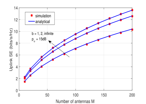
Figure 2: Simulated and analytical SEs of massive MIMO with uniform-resolution ADCs versus the number of antennas $M$.

Fig. 2 shows the uplink SE versus the number of antennas with uniform-resolution ADCs as $1,2,$ infinite bits. The number of users is 8. We can see that, in all cases of the number of antennas, the simulation results match very well the analytical results. With only $2$ bits, the SE nearly approaches that with ideal ADCs (infinite resolution). For fixed values of ${p_{u}}$, all curves grow without bound as $M$ increases, while for variable values of ${p_{u}}={{{E_{u}}}\mathord{\left/{\vphantom{{{E_{u}}}M}}\right.\kern-1.2pt}M}$, the corresponding curves eventually saturate as $M$ increases. Note that ${E_{u}}$ is set as 30dB.

V Conclusion

In this paper, AQNM is used to model the effect of the low-resolution ADCs. Based on the AQNM, we propose a high-performance MMSE receiver for massive MIMO systems with low-resolution ADCs, which can suppress both AWGN and quantization noise at the same time. Using the proposed MMSE receiver and random matrix theory, we derive the asymptotic equivalent of the uplink SE. Numerical results show that the asymptotic equivalent is very tight. Moreover, the loss of the uplink SE brought by the low-resolution ADCs can be compensated by increasing the number of antennas at BS.

Appendix A

Theorem 1 ([10]): Let ${\bf{U}}\in{{\mathbb{C}}^{M\times M}}$ and ${\bf{Z}}\in{{\mathbb{C}}^{M\times M}}$ be Hermitian nonnegative definite and ${\bf{H}}\in{{\mathbb{C}}^{M\times K}}$ be random with independent columns ${{\bf{h}}_{k}}\sim{\cal{C}}{\cal{N}}\left({0,\frac{1}{M}{{\bf{R}}_{k}}}\right)$. Assume that ${\bf{U}}$ and ${{\bf{R}}_{k}}\left({k=1,2,\ldots,K}\right)$, have uniformly bounded spectral norms (with respect to $M$). Then when $M,K\to\infty$ with fixed ratio and any $\rho>0$,

$$\frac{1}{M}{\bf{tr}}\left({{\bf{U}}{{\left({{\bf{H}}{{\bf{H}}^{H}}+{\bf{Z}}+\rho{{\bf{I}}_{M}}}\right)}^{-1}}}\right)-\frac{1}{M}{\bf{tr}}\left({{\bf{US}}\left(\rho\right)}\right)\overset{a.s.}{\longrightarrow}{0},$$

where ${\bf{S}}\left(\rho\right)={\left({\frac{1}{M}\sum\nolimits_{k=1}^{K}{\frac{{{{\bf{R}}_{k}}}}{{1+{\delta_{k}}\left(\rho\right)}}}+{\bf{Z}}+\rho{{\bf{I}}_{M}}}\right)^{-1}}$ and ${\delta_{k}}\left(\rho\right)$ is defined as ${\delta_{k}}\left(\rho\right)={\lim_{t\to\infty}}\delta_{k}^{t}\left(\rho\right)$, $k=1,\ldots,K$, where

$$\delta_{k}^{\left(t\right)}\left(\rho\right)=\frac{1}{M}{\bf{tr}}\left({{{\bf{R}}_{k}}{{\left({\frac{1}{M}\sum\limits_{i=1}^{K}{\frac{{{{\bf{R}}_{i}}}}{{1+\delta_{i}^{\left({t-1}\right)}\left(\rho\right)}}}+{\bf{Z}}+\rho{{\bf{I}}_{M}}}\right)}^{-1}}}\right),$$

for $t=1,2,\ldots,$ with initial value $\delta_{k}^{\left(0\right)}={1\mathord{\left/{\vphantom{1\rho}}\right.\kern-1.2pt}\rho}$ for all $k$.

Theorem 2 ([10]): Let ${\Theta}\in{{\mathbb{C}}^{M\times M}}$ be Hermitian nonnegative definite with uniformly bounded spectral norm (with respect to $M$). Under the same conditions as in Theorem 1,

$$\frac{1}{M}{\bf{tr}}\left({{\bf{U}}{{\bf{A}}^{-1}}\Theta{{\bf{A}}^{-1}}}\right)-\frac{1}{M}{\bf{tr}}\left({{\bf{US^{\prime}}}\left(\rho\right)}\right)\overset{a.s.}{\longrightarrow}{0},$$

where ${\bf{A}}={\bf{H}}{{\bf{H}}^{H}}+{\bf{Z}}+\rho{{\bf{I}}_{M}}$ and ${\bf{S^{\prime}}}\left(\rho\right)\in{{\mathbb{C}}^{M\times M}}$ is

$${\bf{S^{\prime}}}\left(\rho\right)={\bf{S}}\left(\rho\right)\Theta{\bf{S}}\left(\rho\right)+{\bf{S}}\left(\rho\right)\frac{1}{M}\sum\limits_{k=1}^{K}{\frac{{{{\bf{R}}_{k}}{{\delta^{\prime}}_{k}}\left(\rho\right)}}{{{{\left({1+{\delta_{k}}\left(\rho\right)}\right)}^{2}}}}{\bf{S}}\left(\rho\right)}.$$

${\bf{S}}\left(\rho\right)$ and ${\delta_{k}}\left(\rho\right)$ are defined in Theorem 1. And ${\bf{\delta^{\prime}}}\left(\rho\right)={\left[{{{\delta^{\prime}}_{1}}\left(\rho\right),\ldots,{{\delta^{\prime}}_{K}}\left(\rho\right)}\right]^{T}}$ is calculated as ${\bf{\delta^{\prime}}}\left(\rho\right)={\left({{{\bf{I}}_{M}}-{\bf{J}}\left(\rho\right)}\right)^{-1}}{\bf{v}}\left(\rho\right)$, where

$$\begin{array}[]{l}{\left[{{\bf{J}}\left(\rho\right)}\right]_{kl}}=\frac{{\frac{1}{M}{\bf{tr}}\left({{{\bf{R}}_{k}}{\bf{S}}\left(\rho\right){{\bf{R}}_{l}}{\bf{S}}\left(\rho\right)}\right)}}{{M{{\left({1+{\delta_{l}}\left(\rho\right)}\right)}^{2}}}},{\rm{1}}\leq k,l\leq K\\ {\left[{{\bf{v}}\left(\rho\right)}\right]_{k}}=\frac{1}{M}{\bf{tr}}\left({{{\bf{R}}_{k}}{\bf{S}}\left(\rho\right)\Theta{\bf{S}}\left(\rho\right)}\right),1\leq k\leq K.\end{array}$$

References

• [1] J. G. Andrews et al., β€œWhat will 5G be?,” IEEE J. Sel. Areas Commun., vol. 32, no. 6, pp. 1065-1082, Jun. 2014.
• [2] H. Q. Ngo, E. G. Larsson, and T. L. Marzetta, β€œEnergy and spectral efficiency of very large multiuser MIMO systems,” IEEE Trans. Commun., vol. 61, no. 4, pp. 1436-1449, Apr. 2013.
• [3] B. Le, T. Rondeau, J. Reed, and C. Bostian, β€œAnalog-to-digital converters,” IEEE Signal Process. Mag., vol. 22, no. 6, pp. 69-77, Nov. 2005.
• [4] Q. Bai and J. A. Nossek, β€œEnergy efficiency maximization for 5G multiantenna receivers,” Trans. Emerging Telecommun. Technol., vol. 26, no. 1, pp. 3-14, Jan. 2015.
• [5] L. Fan, S. Jin, C.-K. Wen, and H. Zhang, β€œUplink achievable rate for massive MIMO systems with low-resolution ADC,” IEEE Commun. Lett., vol. 19, no. 12, pp. 2186-2189, Dec. 2015.
• [6] J. Zhang, L. Dai, S. Sun and Z. Wang, β€œOn the spectral efficiency of massive MIMO systems with low-resolution ADCs,” IEEE Commun. Lett., vol. 20, no. 5, pp. 842-845, May 2016.
• [7] N. Liang and W. Zhang, β€œMixed-ADC massive MIMO,” IEEE J. Sel. Areas Commun., vol. 34, no. 4, pp. 983-997, Apr. 2016.
• [8] J. Zhang, L. Dai, Z. He, J. Shi and X. Li, β€œPerformance analysis of mixed-ADC massive MIMO systems over Rician fading channels,” IEEE J. Sel. Areas Commun., vol. 35, no. 6, pp. 1327-1338, Jun. 2017.
• [9] Y. Dong and L. Qiu, β€œSpectral efficiency of massive MIMO systems with low-resolution ADCs and MMSE receiver,” IEEE Commun. Lett., Apr. 2017.
• [10] S. Wagner, R. Couillet, M. Debbah, and D. T. M. Slock, ”Large system analysis of linear precoding in correlated MISO broadcast channels under limited feedback,” IEEE Trans. Inf. Theory, vol. 58, no. 7, pp. 4509-4537, Jul. 2012.