Structure of the Milky Way stellar halo out to its outer boundary with blue horizontal-branch stars

Abstract

We present the structure of the Milky Way stellar halo beyond Galactocentric distances of $r=50$ kpc traced by blue horizontal-branch (BHB) stars, which are extracted from the survey data in the Hyper Suprime-Cam Subaru Strategic Program (HSC-SSP). We select BHB candidates based on $(g,r,i,z)$ photometry, where the $z$-band is on the Paschen series and the colors that involve the $z$-band are sensitive to surface gravity. About 450 BHB candidates are identified between $r=50$ kpc and 300 kpc, most of which are beyond the reach of previous large surveys including the Sloan Digital Sky Survey. We find that the global structure of the stellar halo in this range has substructures, which are especially remarkable in the GAMA15H and XMM-LSS fields in the HSC-SSP. We find that the stellar halo can be fitted to a single power-law density profile with an index of $\alpha\simeq 3.3$ ($3.5$) with (without) these fields and its global axial ratio is $q\simeq 2.2$ ($1.3$). Thus, the stellar halo may be significantly disturbed and be made in a prolate form by halo substructures, perhaps associated with the Sagittarius stream in its extension beyond $r\sim 100$ kpc. For a broken power-law model allowing different power-law indices inside/outside a break radius, we obtain a steep power-law slope of $\alpha\sim 5$ outside a break radius of $\simeq 100$ kpc ($200$ kpc) for the case with (without) GAMA15H and XMM-LSS. This radius of $200$ kpc might be as close as a halo boundary if there is any, although larger BHB sample is required from further HSC-SSP survey to increase its statistical significance.

1 Introduction

Structure and evolution of a faint, diffuse stellar halo surrounding a disk galaxy like our own Milky Way are still enigmatic, although it is one of the basic, ancient galactic components. A stellar halo is especially important as it preserves fossil records of galaxy formation through hierarchical merging and past accretion events because of its long dynamical time, compared to dynamically well-relaxed, bright disk components. This is the reason why, despite its tiny fraction of stellar masses in a galaxy and the difficulty to identify it, a stellar halo has been paid special attention to researchers since the seminal papers by Eggen, Lynden-Bell & Sandage (1962), Searle & Zinn (1978) and subsequent studies (see reviews, e.g., Helmi (2008); Ivezić, Beers & Juric (2012); Feltzing & Chiba (2013); Bland-Hawthorn & Freeman (2014)).

While the structure of the Milky Way stellar halo is traced by several means, e.g., stellar kinematics, the simple method is to count and map out its bright tracers, such as red giant-branch (RGB) stars, RR Lyrae (RRL) and blue horizontal-branch (BHB) stars, which can be observable even at the outskirts of the Milky Way halo. The latter, RRL and BHB stars are especially advantageous in this purpose, as their absolute magnitudes and thus distances can be calibrated in a straightforward way. Based on the assembly and analysis of these halo tracers, some basic structure of the stellar halo has been revealed out to a few tens kpc and sometimes $r\sim 100$ kpc from the Galactic center; the stellar halo consists of a general smooth component and irregular substructures (e.g., Sluis & Arnold (1998); Yanny et al. (2000); Chen et al. (2001); Sirko et al. (2004); Newberg & Yanny (2005); Jurić et al. (2008); Keller et al. (2008); Sesar et al. (2011); Deason et al. (2011); Xue et al. (2011); Deason et al. (2014); Cohen et al. (2015, 2017); Vivas et al. (2016); Slater et al. (2016); Xu et al. (2018); Deason et al. (2018); Hernitschek et al. (2018)).

The smooth halo component is often modeled as a power-law radial profile with an index $\alpha$ and an axial ratio $q$. Previous works have attempted to obtain these density parameters and reached a rough agreement of $2<\alpha<4$ and $0.4<q<0.8$, namely rapidly falling density profile with an oblate to nearly round shape (Sluis & Arnold, 1998; Yanny et al., 2000; Chen et al., 2001; Newberg & Yanny, 2005; Jurić et al., 2008; Sesar et al., 2011; Deason et al., 2011; Slater et al., 2016; Xu et al., 2018). Most recently, Hernitschek et al. (2018) presented the density profile of RR Lyrae stars selected from the Pan-STARRS1 survey, which probe the most outer halo of the Galaxy out to Galactocentric distance of $r=135$ kpc ever done using these variables, and obtained $\alpha=4.4$ and $q=0.9$ over $20<r<135$ kpc. There are also evidence for a non-monotonous halo structure, such that these halo parameters vary with radius, from a flattened shape in the inner parts to a less-flattened shape with a steeper slope in the outer parts (Hartwick, 1987; Deason et al., 2014; Cohen et al., 2015, 2017; Hernitschek et al., 2018). The stellar halo also shows evidence for a wealth of substructures, especially revealed by the Sloan Digital Sky Survey (SDSS), including the Sagittarius (Sgr) stream, Virgo overdensity and the Hercules-Aquila Cloud (Ibata et al., 1995; Belokurov et al., 2006; Jurić et al., 2008). These lines of evidence suggest that the formation of the stellar halo is indeed through a series of hierarchical merging/accretion events and this process is continuing perhaps even in the present day.

While most of the previous works investigate the stellar halo out to $r$ of a few tens kpc to $\sim 100$ kpc, it is still well below a virial radius of a MW-sized dark matter halo, typically $200-300$ kpc. Also, we have not yet identified any sharp outer edge of the stellar halo if there is any, so this ancient component may be much extended without any clear boundary, depending on the recent merging/accretion history over past billion years (Bullock & Johnston et al., 2005; Deason et al., 2014). It is thus our motivation of this paper to investigate the structure of the stellar halo in its outskirts of $r>100$ kpc. Our work is based on distant BHB stars from the ongoing Subaru Strategic Program (SSP) using Hyper Suprime-Cam (HSC) (Aihara et al., 2018a, b, see for the details of HSC-SSP). HSC is a new prime-focus camera on Subaru with a 1.5 deg diameter field of view (Miyazaki et al., 2018; Komiyama et al., 2018; Furusawa et al., 2018; Kawanomoto et al., 2018), whereby enabling sciences with wide and deep imaging data, including the current work of halo mapping out to its outer boundary.

This paper is organized as follows. In Section 2, we present the data that we utilize here and the method for the selection of BHB candidates based on multi-photometry data. The spatial distribution of these BHB candidates and the method for deriving the radial density profile are also described. Section 3 is devoted to the results and discussion of our maximum likelihood analysis for the BHB candidates. We derive the parameters, $\alpha$ and $q$, for the radial profile of the stellar halo at $r=50-300$ kpc. Finally, our conclusions are drawn in Section 4.

Observed Regions with HSC-SSP Region RA DEC $l$ b adopet area (deg) (deg) (deg) (deg) (deg²) XMM-LSS 35 $-5$ 170 $-59$ 60 WIDE12H 180 0 276 60 28 WIDE01H 19 0 136 $-62$ 0 VVDS 337 0 65 $-46$ 48 GAMA15H 217 0 347 54 85 GAMA09H 135 0 228 28 90 HECTOMAP 242 43 68 47 20 AEGIS 216 51 95 60 2

2 Data and Method

2.1 HSC-SSP data

This work is based on the imaging data of HSC-SSP survey in its Wide layer, which is aimed at observing $\sim 1,400$ deg² in five photometric bands ($g$, $r$, $i$, $z$, and $y$) (for details, see Aihara et al. (2018a, b)). We use data from the internal s16a data release, which covers six fields along the celestial equator, named XMM-LSS around at (RA, DEC) $=(35^{\circ},-5^{\circ})$, WIDE12H at ($180^{\circ}$, $0^{\circ}$), WIDE01H at ($19^{\circ}$, $0^{\circ}$), VVDS at ($337^{\circ}$, $0^{\circ}$), GAMA15H at ($217^{\circ}$, $0^{\circ}$), and GAMA09H at ($135^{\circ}$, $0^{\circ}$) and a field around (RA,DEC)$=(242^{\circ},43^{\circ})$ (HECTOMAP) as well as a calibration field around (RA,DEC)$=(216^{\circ},51^{\circ})$ (AEGIS) at the Wide depth, amounting to $\sim 300$ deg² in total (Table 1). Since WIDE01H has no $i$ and $z$-band data, we don’t use this region. The target 5$\sigma$ point-source limiting magnitudes are ($g$, $r$, $i$, $z$, $y$) = (26.5, 26.1, 25.9, 25.1, 24.4) mag. The HSC data are processed with hscPipe v4.0.1, a branch of the Large Synoptic Survey Telescope pipeline (Ivezić et al., 2008; Jurić et al., 2015) calibrated against Pan-STARRS1 photometry and astrometry (Schlafly et al., 2012; Tonry et al., 2012; Magnier et al., 2013). All the photometry data are corrected for the mean Galactic foreground extinction, $A_{V}$ (Schlegel et al., 1998).

In this paper, for the selection of BHBs by the method described below, we utilize $g$, $r$, $i$ and $z$-band data for point sources selected using the extendedness parameter from the pipeline, namely extendedness$=0$ for point sources and extendedness$=1$ for extended images like galaxies. For more details of the description of this parameter, see the data release paper by Aihara et al. (2018b). However, this star/galaxy classification becomes uncertain for faint sources. As detailed in Aihara et al. (2018b), the contamination, defined as the fraction of galaxies classified by HST/ACS among HSC-classified stars, is close to zero at $i<23$, but increases to $\sim 50\%$ at $i=24.5$ at the median seeing of the survey ($0.6$ arcsec). In what follows of Section 2, we adopt point sources with $i\leq 24.5$ and investigate the possible effect of the contamination by faint galaxies.

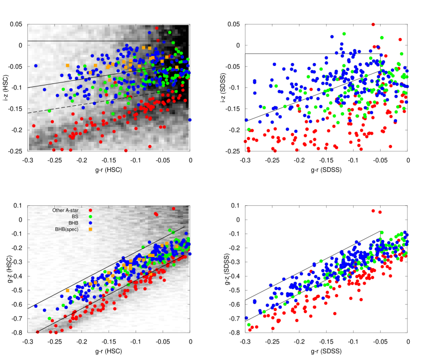
Figure 1: Color-color diagrams for the selection of BHB stars in the $g-r$ vs. $i-z$ space (upper panel) and the $g-r$ vs. $g-z$ space (lower panel). Left and right panels correspond to the HSC and SDSS filter systems, respectively. Green and blue points indicate stars classified as BS and BHB candidates, respectively, whereas red points are other A-colored point sources based on SDSS’s ($u,g,r$)-band selection (Yanny et al., 2000). Orange squares show BHB stars selected from spectroscopy by Xue et al. (2011). In left panels with the HSC filter system, black dots are all of the point-source data in HSC-SSP and areas enclosed by solid lines denote the fiducial selection region for BHB stars against BSs, white dwarfs and quasars adopted in this work. The dashed lines in the blue side of $i_{\rm SDSS}-z_{\rm SDSS}$ (upper left panel) is also employed to examine the effects of the contamination by BS stars. In the right panel with the SDSS filter system, solid lines show the selection of BHB stars proposed by Vickers et al. (2012).

2.2 Selection of BHB stars

Candidate BHB stars are often selected using their ultraviolet light as a surface gravity indicator to distinguish from A-type stars. This is mainly due to the Balmer jump at 365 nm which is sensitive to surface gravity. For instance, Sirko et al. (2004) adopt the $u$-band data in the SDSS imaging survey and set the color cut in the $g-r$ vs. $u-g$ for the selection of BHB stars as suggested by Lenz et al. (1998). This method however cannot be applied due to the lack of $u$-band data in HSC.

Lenz et al. (1998) also suggest the selection in $i-z$ space which is caused by the Paschen features and is sensitive to surface gravity. Vickers et al. (2012) develop this selection method using the $z$ band in the $i-z$ vs. $g-r$ diagram for the removal of A-type stars, white dwarfs and quasars, and also use the $g-z$ vs. $g-r$ color for the removal of remaining quasars. According to Vickers et al. (2012), who adopt 10 globular clusters in the SDSS photometry showing pronounced BHBs for the test, their selection method provides BHBs with $\sim 77$% pure and $\sim 51$% complete, whereas $u$-based color cut selects BHBs with $\sim 74$% pure and $\sim 57$% complete.

Vickers et al. (2012) adopted the SDSS filter system to define the selection regions of BHBs in both the $i-z$ vs. $g-r$ color and the $g-z$ vs. $g-r$ color diagrams. Since the $z$-band filter response of SDSS is different from that of HSC, we define new selection regions using the HSC filter system. For this purpose, we select the SDSS photometric data crossmatched with the HSC data available here, in the restricted color range for A-type stars:

$$-0.3<g_{\rm SDSS} - r_{\rm SDSS}<0$$ (1)

$$-0.25<i_{\rm SDSS} - z_{\rm SDSS}<0.05$$ (2)

where the latter roughly corresponds to $0<u_{\rm SDSS}-g_{\rm SDSS}<1.5$, which covers the expected color range for the selection of the BHB stars. We also confine ourselves to $g_{\rm SDSS}<20$ to minimize photometric uncertainties. In Figure 1, we show the $g-r$ vs. $i-z$ and $g-r$ vs. $g-z$ diagrams for both the HSC and SDSS filter systems, together with BHB and non-BHB candidates taken from Yanny et al. (2000) based on the $u$-band selection with the SDSS system. Red points show the sample classified clearly as non-BHB stars, which are located outside the $u_{\rm SDSS}-g_{\rm SDSS}$ range for BHBs. Both blue and green points are the stars, which are located within the color cut box with boundaries $0.8<u_{\rm SDSS}-g_{\rm SDSS}<1.38$ and $-0.3<g_{\rm SDSS}-r_{\rm SDSS}<0.0$, i.e., colors occupied by BHBs (Yanny et al., 2000). It is well known that these BHB candidates contain blue straggler (BS) stars and these high-gravity stars are removed based on the further division in the $u_{\rm SDSS}-g_{\rm SDSS}$ and $g_{\rm SDSS}-r_{\rm SDSS}$ space (Yanny et al., 2000; Deason et al., 2011). Green points denote candidate BSs separated this way, following the color cut shown in Figure 10 of Yanny et al. (2000). Since this classification method based on the photometric data alone is not so strict, we also adopt the spectroscopic SEGUE sample of BHB stars compiled by Xue et al. (2011) and crossmatch this with the current HSC sample. These stars are designated with orange squares in Figure 1. It follows that the BHB candidates selected from the color cut well match those selected from spectroscopy.

We note from the comparison of the left and right panels in Figure 1 that the HSC system enables to separate BHBs and non-BHBs more clearly than SDSS. The reason for this difference is that the HSC $z$-band response is more closely matched with the Paschen series than SDSS $z$-band, which are sensitive to the surface gravity.

In this paper, we adopt BHB selection boxes from the HSC filter system as bounded by solid lines in the left panel of Figure 1. These solid lines are defined as

$$-0.3<g_{\rm HSC} - r_{\rm HSC}<0$$ (3)

$$0.2(g_{\rm HSC}-r_{\rm HSC})-0.04<i_{\rm HSC} - z_{\rm HSC}<0.01$$ (4)

$$2(g_{\rm HSC}-r_{\rm HSC})-0.23<g_{\rm HSC} - z_{\rm HSC}<2(g_{\rm HSC}-r_{\rm HSC})-0.03.$$ (5)

We note that this boundary well covers the spectroscopic sample of BHBs.

In addition, we also examine another selection box with a larger area bounded by a dashed line in the blue side of $i-z$, to investigate the effects of the contamination of BS stars (designated by green points) in the later subsection. In this case, the solid line given as eq.(4) is replaced by the dashed line given as,

$${}0.2(g_{\rm HSC}-r_{\rm HSC})-0.1<i_{\rm HSC}-z_{\rm HSC}<0.01$$ (6)

For the crossmatch, we convert the current HSC filter system to the SDSS one by the formula given as

$$g_{\rm HSC} = g_{\rm SDSS}-a(g_{\rm SDSS}-r_{\rm SDSS})-b$$ (7)

$$r_{\rm HSC} = r_{\rm SDSS}-c(r_{\rm SDSS}-i_{\rm SDSS})-d$$ (8)

$$i_{\rm HSC} = i_{\rm SDSS}-e(r_{\rm SDSS}-i_{\rm SDSS})+f$$ (9)

$$z_{\rm HSC} = z_{\rm SDSS}+g(i_{\rm SDSS}-z_{\rm SDSS})-h,$$ (10)

where $(a,b,c,d,e,f,g,h)=(0.074,0.011,0.004,0.001,0.106,0.003,0.006,0.006)$ and the subscript HSC and SDSS denote the HSC and SDSS system, respectively. These formula, derived by M. Akiyama (private communication, see also Homma et al. (2016)), have been calibrated from both filter curves and spectral atlas of stars (Gunn & Stryker, 1983).

2.3 Contamination of BS stars

The color cuts given in Figure 1 are aimed at clearly separating and selecting BHB stars, but the color-color space defined for these stars suffers from finite contamination from BS stars and other populations to some extent. We thus need to consider and quantify the effects of the contaminants in our selection of BHB stars. For this purpose, we adopt multi-color ($griz$) HSC photometry of an old stellar system such as a globular cluster or dwarf spheroid, from which we select both BHB and BS stars and investigate the efficiency of separating BHB stars using the color cuts given in Figure 1. In this method, we assume that member stars in an old stellar system have similar population properties to those of field halo stars, which we regard is a reasonable working hypothesis.

The Wide layer in the HSC-SSP covers the area containing a dwarf spheroidal galaxy, Sextans, having an extended stellar distribution. We thus adopt this galaxy data for the current purpose. So far, yet only the $grz$ imaging data are available in the current HSC-SSP data set, so to supplement the remaining $i$-band data, we utilize the $gi$-band HSC data of this galaxy taken by our group in the Subaru open-use observing program (Chiba et al. S14B-060I). The cross-matching is made between this and HSC-SSP data using $g$-band photometry for Sextans and the candidate member stars of this galaxy spread over its nominal tidal radius, $r_{t}=83.2$ arcmin, are retrieved with the central position of $({\rm RA},{\rm DEC})=(10:13:02.29,-01:36:53.0)$, position angle of PA$=57.5$ deg and ellipticity of $e=1-b/a=0.29$ (Rodericket al., 2016).

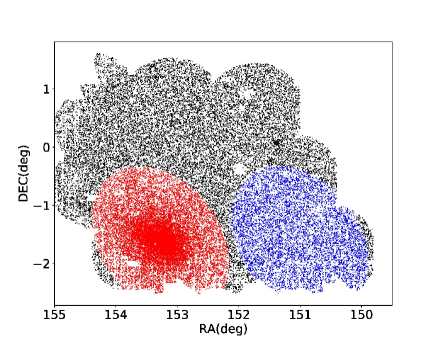
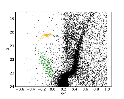
Figure 2: Left: spatial distribution of stars in the HSC-SSP data near a dwarf spheroidal galaxy, Sextans. The candidate member stars in Sextans are designated with red points. Blue points show the field stars outside Sextans but covering the same area. These field stars are utilized for the correction in the estimate of selecting BHB stars. Right: $g$ vs. $g-r$ color diagram of stars in Sextans. Orange and green points denote the selected BHB and BS stars.

The left panel of Figure 2 shows the selected regions of Sextans from HSC-SSP (red points). We also utilize the field stars outside Sextans but distributed over the same area (blue points) for their correction of the following analysis. The right panel of Figure 2 shows the $g$ vs. $g-r$ color-magnitude diagram in Sextans. We then select candidate BHB and BS stars in Sextans at a distance modulus of $m_{g}-M_{g}=19.672$ mag (Rodericket al., 2016) as well as for the selected field regions, defined as $-0.3<g-r<0$ and $19.472<(m_{g}-M_{g})<19.972$ for BHB stars (orange points in the right panel of Figure 2) and $-0.3<g-r<0$ and $19.272<(m_{g}-M_{g})<20.572$ for BS stars (green points), where we use $g$-band absolute magnitudes of BHB and BS stars in equations (11) and (12) as given below. Next, we set the color cuts defined in Figure 1 for these stars and count the number of each stellar population based on these cuts, as summarized in Table 2.3, where $N_{\rm tot}$ is the total number of each of the selected BHB and BS stars, whereas $N_{\rm in}$ and $N_{\rm out}$ are the corresponding number of stars inside/outside the color cuts in Figure 1. For the selection of BHB stars, we obtain the completeness of $\sim 67$% and the purity of $\sim 62$%. These numbers are compared with those for $u$-based color cuts for BHB stars with $\sim 57$% complete and $\sim 74$% pure (Vickers et al., 2012). It is also worth noting that compared with the use of the $z$-band photometry by SDSS with $\sim 51$% complete and $\sim 77$% pure (Vickers et al., 2012), the current method using HSC photometry provides a better completeness of selecting BHB stars. This is because the HSC $z$-band is more closely matched with the Paschen series than the SDSS $z$-band.

BHB and BS stars inside/outside Sextans BHB or BS $N_{\rm tot}$ $N_{\rm in}$ $N_{\rm out}$ Sextans BHB 178 116 62 Sextans BS 411 64 347 field BHB 10 3 7 field BS 43 2 41

2.4 Distance estimate and spatial distribution of BHBs

We adopt the formula for $g$-band absolute magnitudes of BHBs, $M_{g}^{\rm BHB}$, calibrated by Deason et al. (2011),

$$M_{g}^{\rm BHB} = 0.434-0.169(g_{\rm SDSS}-r_{\rm SDSS})$$ (11)

$$+2.319(g_{\rm SDSS}-r_{\rm SDSS})^{2}+20.449(g_{\rm SDSS}-r_{\rm SDSS})^{3}$$

$$+94.517(g_{\rm SDSS}-r_{\rm SDSS})^{4},$$

where both $g$ and $r$ band magnitudes are corrected for interstellar absorption. To estimate the absolute magnitude of BHBs selected from the HSC data, we also use eq.(7) - (10) to translate HSC to SDSS filter system. We then estimate the heliocentric distances and the three dimensional positions of BHBs in rectangular coordinates, $(x,y,z)$, for the Milky Way space, where the Sun is assumed to be at (8.5,0,0) kpc. To consider the finite effect of contamination from BS stars as shown below, we adopt their $g$-band absolute magnitudes, $M_{g}^{\rm BS}$, given by Deason et al. (2011),

$$M_{g}^{\rm BS}=3.108+5.495(g_{\rm SDSS}-r_{\rm SDSS}).$$ (12)

Figure 3 shows the three dimensional map of BHB candidates in the current sample. Different colors denote different survey fields. As is clear, the area in each survey region is yet limited to $\sim 50$ deg², so the selected BHB stars are distributed within a pencil cone; AEGIS is confined to the smallest region for its calibration purpose, so only one BHB is identified in this field.

Figure 3: The spatial distribution of BHB candidates on the Milky Way $x-y$ plane (left panel) and $x-z$ plane (right panel) , where the Sun is located at $(8.5,0,0)$ kpc and the Galactic plane is defined by the $xy$ plane. BHBs in each of the survey fields are plotted with different colors. Here we only use $i\leq 23$ mag sample which excludes the contamination of galaxies.

In the GAMA15H field, there exists the so-called Virgo overdensity covering a distance from $6$ to $44$ kpc and beyond (Jurić et al., 2008; Vivas et al., 2016), which yields the higher number density of BHBs than in other fields. As shown below (cyan line for GAMA15H in Figure 4), in addition to the structure associated with the Virgo overdensity, we find a secondary structure at $r=100-200$ kpc, which would largely affect the determination of the smooth-halo structure. Also, it is noted that the XMM-LSS field includes a part of the bright stream which exists at $r=20-40$ kpc (Koposov et al., 2012). However, as also shown below (red line in Figure 4), such a substructure does not clearly appear in the current sample, because our survey region is basically beyond the corresponding radial range. Since there may exist some unavoidable effects from this field, we conservatively exclude not only GAMA15H but also XMM-LSS from the sample when we examine the effects of these known halo substructures on the determination of the density profile of the halo.

Figure 4 shows the cumulative number distribution $N(<r)$ of BHB candidates as a function of the radial distance from the center, $r$, in each of the survey fields (colored curve). Black curve shows the distribution by summing up all fields. Several characteristic features are notable as summarized below.

• In all fields, there exists an excess of BHB candidates at $r$ beyond $\sim 300$ kpc, which corresponds to $g$-band magnitude fainter than $\sim 23$ mag or $i$-band magnitude fainter than $\sim 23.4$ mag at which galaxy contamination starts to come in (Aihara et al., 2018b). This suggests that the excess feature is due to the contamination of faint galaxies and that to avoid this contamination effect, we should confine ourselves to BHB candidates with $i\leq 23$ mag or $r\leq 300$ kpc.

• In all fields, there exists a lack of BHB candidates at $r$ below $\sim 30$ kpc, which corresponds to $g$-band magnitude brighter than $\sim 18$ mag. Note that such bright objects are often saturated in the HSC-SSP data (Aihara et al., 2018b).

• GAMA15H shows the highest cumulative number of BHB candidates most probably due to the presence of halo substructures including the Virgo overdensity and beyond.

• All fields show similar radial profiles in general.

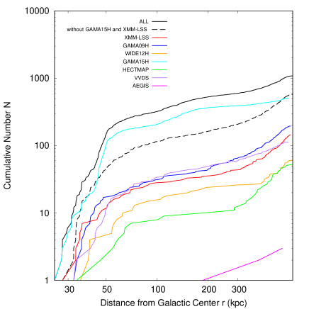
Figure 4: Cumulative number distribution of BHB candidates as a function of the radial distance, $r$, from the center. We note that an excess of BHB candidates at $r$ beyond $\sim 300$ kpc is due to the contamination of faint galaxies in the sample. Here we adopt the faint data with $i\leq 24.5$ mag to demonstrate the effect of contamination from background galaxies.

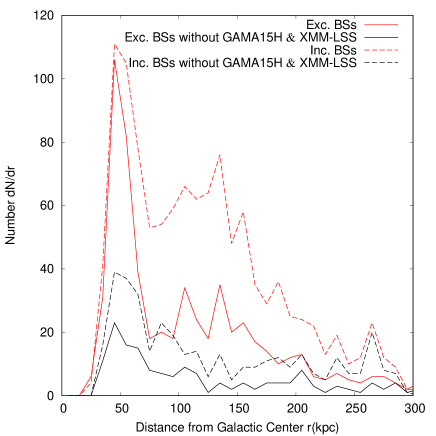
Figure 5: Differential number distributions of variously selected stellar populations as a function of $r$. Red (black) solid lines correspond to our BHB candidates inside the selection box bouded by solid lines in the left panel of Figure 1 with (without) GAMA15H and XMM-LSS. Red (black) dashed lines correspond to both BHB ad BS candidates by adopting the selection box bounded by a dashed line in Figure 1 with (without) GAMA15H and XMM-LSS.

In Figure 5, we show the differential distributions of variously selected stellar populations as a function of $r$, namely the radial density profile $dN(<r)/dr$. Red (black) solid lines are devoted to our BHB candidates inside the selection box bounded by solid lines in the left panel of Figure 1 with (without) GAMA15H and XMM-LSS. There is a peak at $r=50-60$ kpc, beyond which the sample of BHB candidates is sufficient enough to enable the derivation of the intrinsic density profile. This density peak appears to be largely provided by the Virgo overdensity, since its amplitude is significantly reduced when GAMA15H and XMM-LS are excluded (black solid line). Also, we note that the BHB sample with GAMA15H and XMM-LS (red solid line) shows a secondary structure revealed at $r=100-200$ kpc, whereas that without including these fields (black solid line) shows no corresponding feature. This may imply that the secondary feature at $r=100-200$ kpc is caused by some finite contamination of faint BS stars (with about 2 mag fainter luminosities than BHBs) located in the Virgo overdensity and the bright stream at much inner radii. To assess this, we consider many of BS candidates in addition to BHB ones by adopting the selection box bounded by a dashed line in Figure 1 and the results for $dN(r)/dr$ are shown with red (black) dashed lines with (without) GAMA15H and XMM-LSS in Figure 5. It clearly follows that the secondary feature reported above is much enhanced by including BS candidates, thereby suggesting that this feature is associated with the substructures including the Virgo overdensity and bright stream for these faint stars. We note from the black dashed line that the sample without including GAMA15H and XMM-LS can exclude the effect of these substructures.

It is also worth remarking that for the case of excluding BS stars without including GAMA15H and XMM-LSS (black solid line), there is no signature of a sharp outer edge or rapidly falling density profile beyond $r=50$ kpc. This is in contrast to the results of Deason et al. (2014), who propose, using their BHB sample, a steep power-law slope at $r$ beyond 50 kpc, i.e., $\rho\propto r^{-\alpha}$ with $\alpha\geq 6$, but in agreement with those of Cohen et al. (2017) using RR Lyrae, suggesting $\alpha\simeq 4$ for $50<r<100$ kpc. This density profile with a power-law slope of $-3.5$ to $-5$, at least at $r\leq 85$ kpc, is also suggested from recent works by Slater et al. (2016) ($\alpha=3.5$) and Xu et al. (2018) ($\alpha=5.0$) using K giants selected from SDSS and LAMOST, respectively. Most recently, using the public release of HSC-SSP data over $\sim 100$ deg² and selecting BHB candidates, Deason et al. (2018) found a continuation of a $\alpha=4$ power law from the inner halo when excluding the Sgr stream even beyond 50 kpc.

Based on these general properties of the sample of BHB candidates, we investigate their spatial structure in the range of $50\leq r\leq 300$ kpc using the sample with $i\leq 23$ mag. We also consider the case with and without including GAMA15H and XMM-LSS to obtain the effect of substructures in this sample.

2.5 Maximum likelihood method for getting the radial density profile

To perform Maximum Likelihood analysis for deriving the most likely radial density profile of the BHB stars selected here, while taking account the finite effect of contamination from BS stars, we adopt and follow the methodology given by Deason et al. (2014). First, based on the experiments for estimating the contaminants given above, we define that the membership probabilities of BHB and BS stars, $p(griz|{\rm BHB})$ and $p(griz|{\rm BS})$ based on the $griz$ photometry, are given as the completeness of including the respective stars in the color cuts. Second we assume that the ratio between the number of BHB and that of BS stars remains constant with magnitude, where the fraction of each stellar population relative to the total number of BHB and BS stars is given as $f_{\rm BHB}$ and $f_{\rm BS}$, respectively.

Then, for the volume densities of $\rho_{\rm BHB}(m_{g}-M_{g}^{\rm BHB},l,b)$ and $\rho_{\rm BS}(m_{g}-M_{g}^{\rm BS},l,b)$ for BHB and BS stars, respectively, we define the probability distribution and log-likelihood of

$$P = p(griz|{\rm BHB})\frac{f_{\rm BHB}}{V_{\rm BHB}}\rho_{\rm BHB}(m_{g}-M_{g}^{\rm BHB},l,b)D^{3}_{\rm BHB}$$ (13)

$$+p(griz|{\rm BS})\frac{f_{\rm BS}}{V_{\rm BS}}\rho_{\rm BS}(m_{g}-M_{g}^{\rm BS},l,b)D^{3}_{\rm BS}$$

$$\log L = \sum_{i=1}^{N_{\rm tot}}\log P$$ (14)

where the subscript $i$ denotes each star in the current sample. $D_{\rm BHB}$ and $D_{\rm BS}$ are distance estimates for BHB and BS stars, respectively, and $V_{\rm BHB}$ and $V_{\rm BS}$ denote the volumes subtended by the respective stars, which are derived by integrating over the interval of $18.5<i<23$ mag at a color of $(g-r)=-0.05$. $M_{g}^{\rm BHB}$ and $M_{g}^{\rm BS}$ for the absolute magnitudes of BHB and BS stars, respectively, are given in equations (11) and (12).

In this work, we consider two different models for the radial density profile of BHB stars as a halo tracer. The model for a single power-law profile is given in cylindrical coordinates $(R,z)$ as

$$\rho(R,z)=\rho_{0}R_{\odot}^{\alpha}\left[R^{2}+\frac{z^{2}}{q^{2}}\right]^{-\alpha/2},$$ (15)

where $\rho_{0}$ is the density at the position of the Sun $(R,z)=(R_{\odot},0)$ with $R_{\odot}=8.5$ kpc, and $\alpha$ and $q$ denote the power-law index and axial ratio of the radial density profile, respectively. @Another model is a broken power-law profile given as

$$\rho(R,z)=\left\{\begin{array}[]{rl}\rho_{0}R_{\odot}^{\alpha}r_{q}^{-{\alpha}_{\rm in}},&\qquad{\rm for}\ r_{q}\leq r_{b}\\ \rho_{0}R_{\odot}^{\alpha}r_{b}^{{\alpha}_{\rm out}-{\alpha}_{\rm in}}r_{q}^{-{\alpha}_{\rm out}},&\qquad{\rm for}\ r_{q}>r_{b}\end{array}\right.$$

where $r_{q}=\sqrt{R^{2}+z^{2}/q^{2}}$.

We derive the most likely set of parameters $(\alpha,q)$ for a single power-law model and $(\alpha_{\rm in},\alpha_{\rm out},r_{b},q)$ for a broken power-law model by maximizing $L$, $L_{\rm max}$, and estimate their confident intervals from $F=-2\ln L/L_{\rm max}$ provided $F$ has a $\chi^{2}$ distribution for 2 and 4 degrees of freedom for these models, respectively.

3 Results and Discussion

We adopt the sample of BHB candidates with $i\leq 23$ mag in all survey fields, select those in the range of $50\leq r\leq 300$ kpc, and perform the maximum likelihood analysis as described in the previous section. The results are summarized in Table 3 and 3.

Maximum Likelihood results for a single power-law model Inclusion of GAMA15H and XMM-LSS $\alpha$ $q$ $\ln L$ with $3.27^{+0.17}_{-0.17}$ $2.17^{+0.34}_{-0.30}$ $-110.25$ without $3.51^{+0.36}_{-0.40}$ $1.34^{+0.66}_{-0.38}$ $5.24$

Maximum Likelihood results for a broken power-law model Inclusion of GAMA15H and XMM-LSS $\alpha_{\rm in}$ $\alpha_{\rm out}$ $r_{b}$ (kpc) $q$ $\ln L$ with $3.1^{+0.2}_{-0.5}$ $4.7^{+0.7}_{-0.9}$ $105^{+35}_{-25}$ $2.6^{+1.9}_{-0.4}$ $-173.2$ without $3.2^{+0.9}$ $5.3^{+0.7}$ $210$ $1.5^{+2.1}_{-0.5}$ $10.4$

3.1 The global halo structure over 50 to 300 kpc

The left panel in Figure 6 shows, for a single power-law model, confidence contour plots of the likelihood function $L$, when we consider all the relevant sample with the number $N_{\rm tot}=442$. There exists clearly a localized maximum at $\alpha\simeq 3.3$ and $q\simeq 2.2$, suggesting that the stellar halo in this radial range has a largely prolate shape. On the other hand, the right panel in Figure 6 shows the results when GAMA15H and XMM-LSS having notable substructures are excluded in the analysis, where $N_{\rm tot}=122$. Although confident intervals are enlarged due to the small number of the sample, this case reveals the best-fit parameters of $\alpha\simeq 3.5$ and $q\simeq 1.3$, suggesting that while the index $\alpha$ remains similar, the shape of the stellar halo becomes rounder.

Figure 6: Confidence contour plots of the likelihood function $L$ for a single power-law model, when we consider all the relevant BHB sample (left panel) and when GAMA15H and XMM-LSS containing notable halo substructures are excluded (right panel). Cross shows a best-set of parameters with $L_{\rm max}$ and solid lines show the 1$\sigma$, 2$\sigma$ and 3$\sigma$ confidence.

This result, i.e., the largely prolate shape of the halo when GAMA15H and XMM-LSS are included, may be due to the presence of notable substructures related to the Virgo overdensity in GAMA15H. In particular, these substructures also include a part of the Sgr stream, which is formed from a tidally disrupting, polar-orbit satellite, Sgr dwarf. XMM-LSS also includes a part of the Sgr stream. Thus, the anisotropic distribution of this tidal stream may make the stellar halo being prolate in the above fitting process.

To investigate any radial variation of the halo structure in the current sample of BHB candidates, we also consider a broken power-law model for the halo parameterized by $(\alpha_{\rm in},\alpha_{\rm out},r_{b},q)$ (Table 3). It follows that the case with GAMA15H and XMM-LSS yields a change in the density slope at $r_{b}\simeq 100$ kpc, beyond which the density profile is steeper $(\alpha_{\rm out}\simeq 4.7)$ than that in the inner parts $(\alpha_{\rm out}\simeq 3.1)$. We note that in GAMA15H there exist halo substructures associated with the Sgr stream extended up to $r\sim 80$ kpc and this may explain the current result. On the other hand, without including GAMA15H and XMM-LSS, we obtain the break radius of $r_{b}\simeq 200$ kpc and the halo density profile is made somewhat steeper $(\alpha_{\rm out}\simeq 5.3)$ beyond this radius. This radius might be as close as a halo boundary if there is any, which can be formed by the lack of accretion of small galaxies over the past billion years (Bullock & Johnston et al., 2005; Deason et al., 2014), although this is inferred from yet small number statistics. For further insight into a halo boundary, we need a much larger sample with a higher statistical significance, because the BHB sample in outer radii suffers from misclassification with faint background galaxies. Moreover, since the number of the BHB stars by excluding GAMA15H and XMM-LSS is yet small in the current data set, the associated errors in $\alpha_{\rm in}$, $\alpha_{\rm out}$ and $r_{b}$ for this broken power-law model are large and some of them are actually undetermined in this study (Table 3). Thus, the interpretation of the results for this case still needs a great caution.

It is also worth noting that even in this broken power-law model, the shape of the stellar halo at $r>100$ kpc appears largely prolate, especially when GAMA15H and XMM-LSS are included. This result is compared with suggested oblate shapes at $r<50$ kpc derived in previous work, summarized as $\alpha\sim 3.2$ and $q\sim 0.5$ for BHBs at $1<r<20$ kpc (Sluis & Arnold, 1998), $\alpha\sim 2.6$ and $q\sim 0.65$ for BHBs out $\sim 40$ kpc (Deason et al., 2011), and $2<\alpha\leq 4$ and $0.4\leq q\leq 0.8$ in various other work (Yanny et al., 2000; Chen et al., 2001; Newberg & Yanny, 2005; Jurić et al., 2008; Sesar et al., 2011). This may be understood if there exist some substructures associated with the Virgo overdensity and a secondary substructure seen beyond 100 kpc. Indeed, a recent numerical simulation for investigating the effect of the infalling Sgr dwarf from outside (Dierickx & Loeb, 2017) implies that beyond $r\sim 100$ kpc, the presence of tidal debris associated with the Sgr stream is predicted in the direction of GAMA15H. This supports the hypothesis that the larger axial ratio $q$ when GAMA15H is included is due to the effect of the Sgr stream.

3.2 Comparison with Deason et al. (2018)

Recently, Deason et al. (2018) presented their analysis of BHB stars using the public release of the HSC-SSP data over $\sim 100$ deg². Their method for selecting BHB stars is basically the same as that adopted in this work using $griz$ multiband photometry (Vickers et al., 2012), although there are some differences in details in the adopted color cuts of $i-z$ vs. $g-r$ and $g-z$ vs. $g-r$ as well as the total area of the surveyed regions used in the analysis, where we make use of the HSC-SSP data over $\sim 300$ deg² and thus the total number of identified BHB stars is much larger in our work.

For comparison with their work, we make the number counts of BHB stars following their Maximum Likelihood method. Namely, we set, in this work, bins of 0.45 mag in distance modulus over $18.5<g-M_{g}^{\rm BHB}<23$ and count the number of BHB stars in each bin. The probability distribution function in each distance modulus bin is defined as

$$P({\bf x}) = f_{\rm BHB}p({\bf x}|{\rm BHB})+f_{\rm BS}p({\bf x}|{\rm BS})$$ (16)

$$+f_{\rm WD}\left[0.7p({\bf x}|{\rm WD}_{\rm DA})+0.3p({\bf x}|{\rm WD}_{\rm DB})\right]$$

$$+\frac{f_{\rm QSO}}{{\bf x}_{\rm max}-{\bf x}_{\rm min}}$$

where $p({\bf x}|type)$ is a probability distribution of specified stars in $griz$ space, which is assumed as Gaussian, $p({\bf x}|type)=\frac{1}{\sqrt{2\pi\sigma}}\exp(-(x-x_{0})^{2}/2\sigma^{2})$ and ${\bf x}=griz$. The variation of the Gaussian widths, $\sigma$, with magnitude, is given by the sum of the intrinsic widths and the photometric errors of HSC, $\sigma^{2}=\sigma_{\rm intrinsic}^{2}+\sigma^{2}(griz)$, where $\sigma_{\rm intrinsic}$ is kept fixed and taken from Table 1 of Deason et al. (2018). Here, the contributions of QSOs and White Dwarfs (WDs) with DA/DB types are given as their number fractions of $f_{\rm QSO}$ and $f_{\rm WD}$, where the constant contamination from QSOs are assumed and the ratio between these two types of WDs is set to be $7:3$ (Deason et al., 2014). The number counts of BHB stars, $N_{\rm BHB}$, are then obtained in each bin by maximizing the log-likelihood function of

$$\log L=\sum_{i}^{N_{\rm tot}}\log P({\bf x}_{i}).$$ (17)

Figure 7 shows the density profile of BHB stars based on this methodology, where the cases with (without) GAMA15H and XMM-LSS are shown with asterisks (open squares). It follows that the both cases yield a power-law profile with $\alpha$ being $3$ to $4$; There is a tendency that beyond a radius at $r\sim 100$ kpc (200 kpc) with (without) GAMA15H and XMM-LSS, which is basically the same location of a break radius obtained in the previous subsection, the slope appears steeper than $4$, as also inferred from the above experiments. For comparison with Deason et al. (2018), we simply make a $\chi^{2}$ fitting of a power-law density profile of $\rho\propto r^{-\alpha}$ to the data over $50<r<300$ kpc and obtain $\alpha=3.9$ ($3.5$) for the case with (without) GAMA15H and XMM-LSS. These properties of the current BHB sample are generally in agreement with those in Deason et al. (2018) reporting $\alpha\sim 4$ from the same analysis and thus we conclude that both works arrive at basically the same results. We will further examine this broken nature of the density profile using the future HSC data release.

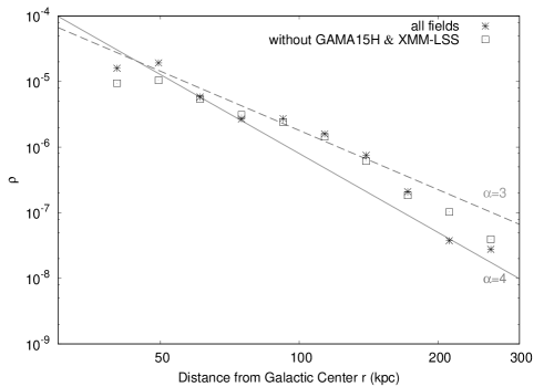
Figure 7: Density profiles of BHB stars with (without) GAMA15H and XMM-LSS based on the Maximum Likelihood method given in equations (16) and (17) are shown with asterisks (open squares). Solid and dashed lines show power-law profiles of $\alpha=3$ and $4$, respectively, for comparison.

3.3 The Sgr stream in GAMA15H and XMM-LSS

In previous section we mention that the Sgr stream is present in GAMA15H and XMM-LSS. Here we investigate the distribution of BHBs relative to that of the Sgr stream in detail. We adopt the heliocentric Sagittarius coordinates, ($\tilde{\Lambda}_{\odot}$, $\tilde{B}_{\odot}$), as defined by Belokurov et al. (2014). As shown in Fig. 8, BHBs in GAMA15H and XMM-LSS are distributed near the Sgr orbital plane (i.e., $|\tilde{B}_{\odot}|<8^{\circ}$). For BHBs in GAMA15H ($60^{\circ}<\tilde{\Lambda}_{\odot}<80^{\circ}$), the Sgr stream is clearly present from $r=$ 50 kpc to 60 kpc. It is also worth remarking that we identify the structure labeled as “feature 3” in Sesar et al. (2017). It should also be mentioned that the Outer Virgo overdensity labeled as “feature 4” in Sesar et al. (2017) is absent in our sample, because this structure exists in the region ($\tilde{B}_{\odot}=-9^{\circ}$) out of GAMA15H. On the other hand, in XMM-LSS ($250^{\circ}<\tilde{\Lambda}_{\odot}<260^{\circ}$), there are no stream-like structures because the current BHB sample is located at larger radii than the Sgr stream (Fig. 8)

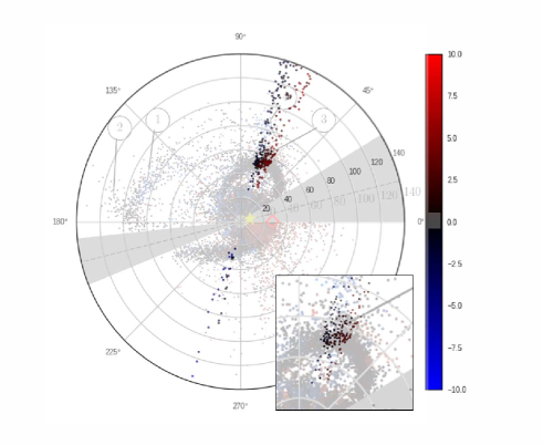
Figure 8: The distribution of BHBs (colored dots) near the Sgr orbital plane (i.e., $|\tilde{B}_{\odot}|<8^{\circ}$) superposed into the map of PS1 RRab stars (gray dots) shown in Figure 1 of Sesar et al. (2017), in which substructures associated with the Sgr stream is clearly seen. The lower right panel shows the enlarged plots in GAMA15H ($60^{\circ}<\tilde{\Lambda}_{\odot}<80^{\circ}$) near the Sgr stream. The color indicates the stars’ angular distance from the Sgr orbital plane.

4 Conclusions

We have extracted BHB candidates in the early survey data of the HSC-SSP over $\sim 300$ deg² based on its $(g,r,i,z)$ photometry, where $z$-band light can be used as a surface gravity indicator of a star against other contaminants. Our purpose with selected BHB stars is to trace and map out the Milky Way stellar halo out to its possible boundary if there is any. About 450 BHB candidates have been identified at Galactocentric distances of 50 to 300 kpc, which corresponds to the $g$-band apparent magnitude of $g=19.2-23.0$ mag if the absolute $g$-band absolute magnitude $M_{g}$ of a BHB is $M_{g}\simeq 0.7$. Thus, HSC enables to detect BHB stars in the outer part of the Milky Way halo which no other surveys can reach.

Based on the maximum likelihood method, we have found that the density structure of the stellar halo at $r=50-300$ kpc when GAMA15H and XMM-LSS having notable substructures are excluded is characterized by a single power-law index $\alpha$ of 3.5 and the axial ratio $q$ of 1.3. This suggests that the stellar halo is slightly prolate in such an outer halo region. When we allow a break radius of $r_{b}$ and different power-law indices inside/outside as $\alpha_{\rm in}$ and $\alpha_{\rm out}$ for the density profile, we obtain a steep slope of $\alpha_{\rm out}\simeq 5.3$ outside $r_{b}\simeq 200$ kpc for the case without GAMA15H and XMM-LSS. On the other hand, halo substructures possibly originated from the tidal stream of the infalling Sgr dwarf dominates the actual halo structure in the outer halo, making it largely prolate with $q>1$.

However, this result is to be assessed using larger BHB sample, because the outer halo region traced by only a few number of BHBs may be yet subject to misclassified contaminations such as A stars and background galaxies. Therefore, the completion of this HSC-SSP survey over $\sim 1,400$ deg² will be important in assessing the current results with higher statistical significance and in exploring further structures of the stellar halo in the Milky Way.

We are grateful to the referee for her/his constructive comments and suggestions that help improve our manuscript substantially. This work is supported in part by JSPS Grant-in-Aid for Scientific Research (B) (No. 25287062) and MEXT Grant-in-Aid for Scientific Research on Innovative Areas (No. 15H05889, 16H01086, 17H01101). N.A. was supported by the Brain Pool Program, which is funded by the Ministry of Science and ICT through the National Research Foundation of Korea (2018H1D3A2000902).

The Hyper Suprime-Cam (HSC) collaboration includes the astronomical communities of Japan and Taiwan, and Princeton University. The HSC instrumentation and software were developed by the National Astronomical Observatory of Japan (NAOJ), the Kavli Institute for the Physics and Mathematics of the Universe (Kavli IPMU), the University of Tokyo, the High Energy Accelerator Research Organization (KEK), the Academia Sinica Institute for Astronomy and Astrophysics in Taiwan (ASIAA), and Princeton University. Funding was contributed by the FIRST program from Japanese Cabinet Office, the Ministry of Education, Culture, Sports, Science and Technology (MEXT), the Japan Society for the Promotion of Science (JSPS), Japan Science and Technology Agency (JST), the Toray Science Foundation, NAOJ, Kavli IPMU, KEK, ASIAA, and Princeton University. This paper makes use of software developed for the Large Synoptic Survey Telescope. We thank the LSST Project for making their code freely available. The Pan-STARRS1 (PS1) Surveys have been made possible through contributions of the Institute for Astronomy, the University of Hawaii, the Pan-STARRS Project Office, the Max-Planck Society and its participating institutes, the Max Planck Institute for Astronomy and the Max Planck Institute for Extraterrestrial Physics, The Johns Hopkins University, Durham University, the University of Edinburgh, Queen’s University Belfast, the Harvard-Smithsonian Center for Astrophysics, the Las Cumbres Observatory Global Telescope Network Incorporated, the National Central University of Taiwan, the Space Telescope Science Institute, the National Aeronautics and Space Administration under Grant No. NNX08AR22G issued through the Planetary Science Division of the NASA Science Mission Directorate, the National Science Foundation under Grant No.AST-1238877, the University of Maryland, and Eotvos Lorand University (ELTE).

References

- Aihara et al. (2018a) Aihara, H., Arimoto, N., Bickerton, S., et al. 2018a, PASJ, 70, S4 (arXiv:1704.05858)
- Aihara et al. (2018b) Aihara, H., Armstrong, R., Bickerton, S., et al. 2018b, PASJ, 70, S8 (arXiv:1702.08449)
- Belokurov et al. (2006) Belokurov, V., Zucker, D. B., Evans, N. W., et al. 2006, ApJ, 647, L11
- Belokurov et al. (2014) Belokurov, V., Koposov, S. E., Evans, N. W., et al. 2014, MNRAS, 437, 116
- Bland-Hawthorn & Freeman (2014) Bland-Hawthorn, J., & Freeman, K., 2014, The Origin of the Galaxy and Local Group, Saas-Fee Advanced Course, Vol. 37 (Springer)
- Bullock & Johnston et al. (2005) Bullock, J. S. & Johnston, K. V. 2005, ApJ, 635, 931
- Chen et al. (2001) Chen, B., Stoughton, C., Smith, J. A., et al. 2001, ApJ, 553, 184
- Cohen et al. (2015) Cohen, J. G., Sesar, B., Banholzer, S., the PTF Collaboration, 2015, IAU General Assembly, 22, 2255152
- Cohen et al. (2017) Cohen, J. G., Sesar, B., Banholzer, S. et al. 2017, ApJ, 849, 150
- Deason et al. (2011) Deason, A. J., Belokurov, V., & Evans, N. W. 2011, MNRAS, 416, 2903
- Deason et al. (2014) Deason, A. J., Belokurov, V., Koposov S. E., Rockosi C. M. 2014, ApJ, 787, 30
- Deason et al. (2018) Deason, A. J., Belokurov, V., Koposov S. E. 2018, ApJ, 852, 118
- Dierickx & Loeb (2017) Dierickx, M. I. P., & Loeb, A. 2017, ApJ, 836, 92
- Eggen, Lynden-Bell & Sandage (1962) Eggen, O. J., Lynden-Bell, D., & Sandage, A. R. 1962, ApJ, 136, 748
- Feltzing & Chiba (2013) Feltzing, S., & Chiba, M. 2013, New Astronomy Reviews, 57, 80
- Furusawa et al. (2018) Furusawa, H., Koike, M., Takata, T., et al. 2018, PASJ, 70S, 3
- Gunn & Stryker (1983) Gunn, J. E., & Stryker, L. L., 1983, ApJS, 52, 121
- Hartwick (1987) Hartwick, F. D. A., 1987, The structure of the Galactic halo, In: Gilmore, G., Carswell, B. (Eds.), The Galaxy, pp.281-290
- Helmi (2008) Helmi, A. 2008, A&ARV, 15, 145
- Hernitschek et al. (2018) Hernitschek, N., Cohen, J. G., Rix, H.-W., et al. 2018, arXiv:1801.10260
- Homma et al. (2016) Homma, D., Chiba, M., Okamoto, S., et al. 2016, ApJ, 832, 21
- Ibata et al. (1995) Ibata, R. A., Gilmore, G., Irwin, M. J. 1995, MNRAS, 277, 781
- Ivezić et al. (2008) Ivezić, Z., Axelrod, T., Brandt, W. N., et al. 2008, AJ, 176, 1
- Ivezić, Beers & Juric (2012) Ivezić, Z., Beers, T. C., & Jurić, M. 2012, ARAA, 50, 251
- Jurić et al. (2008) Jurić, M., Ivezić, Z., Brooks, A., et al. 2008, ApJ, 673, 864
- Jurić et al. (2015) Jurić, M., Kantor, J., Lim, K.-T., et al. 2015, ArXiv e-prints, arXiv:1512.07914
- Kawanomoto et al. (2018) Kawanomoto, S., et al. 2018, in preparation
- Keller et al. (2008) Keller, S. C., Murphy, S., Prior, S., Da Costa, G., & Schmidt, B. 2008, ApJ, 678, 851
- Komiyama et al. (2018) Komiyama, Y., Obuchi, Y., Nakaya, H., et al. 2018, PASJ, 70S, 2
- Koposov et al. (2012) Koposov, S., Belokurov, V., Evans, N. W., et al. 2012, ApJ, 750, 80
- Lenz et al. (1998) Lenz, D. D., Newberg, J., Rosner, R., et al. 1998, ApJS, 119, 121
- Magnier et al. (2013) Magnier, E. A., Schlafly, E., Finkbeiner, D., et al. 2013, ApJS, 205, 20
- Miyazaki et al. (2018) Miyazaki, S., Komiyama, Y., Kawanomoto, S., et al. 2018, PASJ, 70S, 1
- Newberg & Yanny (2005) Newberg, H. J., & Yanny, B. 2005, JPhCS, 47, 195
- Rodericket al. (2016) Roderick, T. A., Jerjen, H., Da Costa, G. S., Mackey, A. D. 2016, MNRAS, 460, 30
- Schlegel et al. (1998) Schlegel, D. J., Finkbeiner, D. P., & Davis, M. 1998, ApJ, 500, 525
- Schlafly et al. (2012) Schlafly, E. F., Finkbeiner, D. P., Jurić, M., et al. 2012, ApJ, 756, 158
- Searle & Zinn (1978) Searle, L., & Zinn, R. 1978, ApJ, 225, 357
- Sesar et al. (2011) Sesar, B, Jurić, M., & Ivezić, Z. 2011, ApJ, 731, 4
- Sesar et al. (2017) Sesar, B, Hernitschek, N, Dierickx, M. I.P., et al. 2017, ApJ, 844, L4 (arXiv:1706.10187)
- Sirko et al. (2004) Sirko, E., Goodman, J., Knapp, G. R., et al. 2004, AJ, 127, 899
- Slater et al. (2016) Slater, C. T., Nidever, D. L., Munn, J. A., Bell, E. F., & Majewski, S. R. 2016, ApJ, 832, 206
- Sluis & Arnold (1998) Sluis, A. P. N., & Arnold, R. A. 1998, MNRAS, 297, 732
- Tonry et al. (2012) Tonry, J. L., Stubbs, C. W., Lykke, K. R., et al. 2012, ApJ, 750, 99
- Vickers et al. (2012) Vickers, J. J., Grebel, E. K., & Huxor, A. P. AJ, 143, 86
- Vivas et al. (2016) Vivas, A. K., Zinn, R., Farmer, J., et al. 2016, ApJ, 831, 165
- Xu et al. (2018) Xu, Y., Liu, C., Xue, X.-X., et al. 2018, MNRAS, 473, 1244
- Xue et al. (2011) Xue, X.-X., Rix, H.-W., Yanny, B., et al. 2011, ApJ, 738, 79
- Yanny et al. (2000) Yanny, B., Newberf, H. J., Kent, S., et al. 2000, ApJ, 540,825