A Class of Control Certificates to Ensure Reach-While-Stay for Switched Systems

Abstract

In this article, we consider the problem of synthesizing switching controllers for temporal properties through the composition of simple primitive reach-while-stay (RWS) properties. Reach-while-stay properties specify that the system states starting from an initial set $I$, must reach a goal (target) set $G$ in finite time, while remaining inside a safe set $S$. Our approach synthesizes switched controllers that select between finitely many modes to satisfy the given RWS specification. To do so, we consider control certificates, which are Lyapunov-like functions that represent control strategies to achieve the desired specification. However, for RWS problems, a control Lyapunov-like function is often hard to synthesize in a simple polynomial form. Therefore, we combine control barrier and Lyapunov functions with an additional compatibility condition between them. Using this approach, the controller synthesis problem reduces to one of solving quantified nonlinear constrained problems that are handled using a combination of SMT solvers. The synthesis of controllers is demonstrated through a set of interesting numerical examples drawn from the related work, and compared with the state-of-the-art tool SCOTS. Our evaluation suggests that our approach is computationally feasible, and adds to the growing body of formal approaches to controller synthesis.

1 Introduction

The problem of synthesizing switching controllers for reach-while-stay (RWS) specifications is examined in this article. RWS properties are an important class, since we may decompose more complex temporal specifications into a sequence of RWS specifications [12]. The plant model is a switched system that consists of finitely many (controllable) modes, and the dynamics for each mode are specified using ODEs. Furthermore, we consider nonlinear ODEs for each mode, including rational, trigonometric, and exponential functions. The goal of the controller is to switch between the appropriate modes, so that the resulting closed loop traces satisfy the specification.

RWS properties specify that a goal set $G$ must be reached by all behaviors of the closed-loop system while staying inside a safe set $S$. Specifically, the state of the system is assumed to be initialized to any state in the set $S$. RWS properties include safety properties (stay inside a safe set $S$), reachability properties (reach a goal set $G$), and “control-to-facet” problems [8, 9].

The controller synthesis is addressed in two phases: (a) formulating a control certificate whose existence guarantees the existence of a non-Zeno switching control law for the given RWS specification, and (b) solving for a certificate of a particular form as a feasibility problem. The control certificates are control Lyapunov-like functions which represent a strategy for the controller to satisfy the specifications. Additionally, this strategy can be effectively implemented as a feedback law using a controller that respects min dwell time constraints. In the second phase, a counterexample guided inductive synthesis (CEGIS) framework [27], — an approach that uses SMT solvers at its core — is used to discover such control certificates. However, this procedure is used off the shelf, building upon the previous work of Ravanbakhsh et al. [23]. This procedure uses a specialized solver for finding a certificate of a given parametric form that handles quantified formulas by alternating between a series of quantifier free formulas using existing SMT solvers [19, 4].

The contributions of the paper are as follows: first, we show that a straightforward formulation of the control certificate for the RWS problem yields an exponential number of conditions, and hence can be computationally infeasible. Next, we introduce a class of control certificates which (i) has a concise logical structure that makes the problem of discovering the certificates computationally feasible; and (ii) we show that such certificates yield corresponding switching strategies with a min-dwell time property unlike the conventional control certificates. Next, we extend our approach to the initialized RWS (IRWS) property that additionally restricts the set of initial conditions of the system using a class of “control zero-ing” barrier functions [34, 37] . Also, a suitable formulation for these functions is provided within our framework. Finally, we provide numerical examples to demonstrate the effectiveness of the method, including comparisons with recently developed state-of-art automatic control synthesis tool SCOTS [26].

1.1 Related Work

The broader area of temporal logic synthesis seeks to synthesize formally guaranteed controllers from the given plant model and specifications. The dominant approach is to build a discrete abstraction of the given plant that is related to the original system [36, 16, 11, 26, 18]. Once a suitable abstraction is found, these approaches use a systematic temporal logic-based controller design approach over the abstraction [33]. The properties of interest in these systems include the full linear temporal logic (LTL) and an efficiently synthesizable subset such as GR(1) [36, 16]. These approaches differ in how the abstraction can be constructed in a guaranteed manner. One class of approaches works by fixing a time step, gridding the state-space, and simulating one point per cell [18, 11, 26, 38, 32]. The resulting abstraction, however, is not always approximately bisimilar to the original system. Nevertheless, conditions such as open loop incremental stability of the plant can be used to obtain bisimilarity [6]. Alternatively, the abstraction can be built without time discretization [21, 16] by considering infeasible transitions. And furthermore, the abstraction can be iteratively refined through a counter-example refinement scheme [20]. Our work here does not directly focus on building abstractions. Rather, our focus is on deductive approaches for a narrow class of temporal logic properties namely RWS properties. Using our approach, control systems for richer properties can be built from solving a series of RWS problems.

Our approach is closely related to work of Habets et al. [7] and Kloetzer et al. [12]. In these methods, an abstraction is obtained by solving local control-to-facet problems instead of reachability analysis. However, continuous feedback is synthesized for each control-to-facet problem. The key difference in this paper is that the control-to-facet problems themselves are solved using switching. Furthermore, we consider initialized problems, where the initial states are also restricted to belong to a set. We find that IRWS problems can often be realized through a controller even when the corresponding RWS problem (for which the initial condition is not restricted) cannot be synthesized.

Another related class of solutions is based on synthesizing “a deductive proof of correctness” simultaneously with “a control strategy”. The goal of these approaches also consists of finding a control certificate, which yields a (control) strategy to guarantee the property. This typically takes the form of a control Lyapunov-like function. The idea of control Lyapunov functions goes back to Artstein [2] and Sontag [28]. The problem of discovering a control Lyapunov function is usually formulated using bilinear matrix inequalities (BMI)  [31]. Also, instead of solving such NP-hard problems, usually alternating optimization (V-K iteration or policy iteration) is used to conservatively find a solution  [31, 5].

Wongpiromsarn et al. [35] discuss verification of temporal logic properties using barrier certificates. For synthesis, Xu et al. [37] discuss conditions for the so-called “control zeroing” barrier functions for safety and their properties. They also, consider their combination with control Lyapunov functions. In this article, we provide an alternative condition that is based on “exponential condition” barrier functions [13] and enforcing a compatibility condition between the control actions suggested by the control barrier and control Lyapunov functions. Also, Dimitrova et. al.  [3] have shown that control certificates can be extended to address more complicated specifications i.e. parity games. While these results show that constraint solving based methods can be applied on more complicated specification, no method of finding such certificates is provided.

The use of SMT solvers in control synthesis has also been well-studied. Taly et. al  [29, 30] use a constraint solving approach to find control certificates for reachability and safety. They adapt a technique known as Counter-Example Guided Inductive Synthesis (CEGIS), originally proposed for program synthesis [27], to solve the control problems using a combination of an SMT solver with numerical simulations. Ravanbakhsh et al. [23] propose a combination of SMT and SDP solvers for finding control certificates. However, their method is only applicable to stability or simple reachability properties, involving the use of a single Lyapunov function. In a subsequent paper, their approach is extended to handle disturbance inputs [24]. The use of SMT solvers to solve for Lyapunov-like functions is used in our paper as well. However, this paper focuses on defining a more tractable class of control certificates for RWS problems. Furthermore, we show how these problems can be composed for more complex temporal objectives. In particular, our use of the CEGIS procedure is not a contribution of this paper. Furthermore, in order to handle nonlinear systems and also to guarantee numerical soundness of these solvers, we use the nonlinear SMT solver dReal [4].

Huang et. al. [10] also propose control certificates to solve the RWS problem for piecewise affine systems, using SMT solvers. Their approach uses piecewise constant functions as control certificates and partitions the state space into small enough cells in order to define such functions. By using this technique, any function can be approximated, which makes the method relatively complete.

As mentioned earlier, past work by Habets et al. and Klutzier et al. [7, 12] build a finite abstraction by repeatedly solving control-to-facet problems. These problems seek to find a feedback law inside a polytope $P$ that guarantees all the resulting trajectories exit $P$ through a specific facet $F$ of $P$. Habets et. al. [8] show necessary and sufficient conditions for the existence of a control strategy for the control-to-facet problem on simplices. This condition is sufficient but not necessary for polytopes. They extract a unique certificate from each problem instance and check whether the condition holds for the certificate. Subsequently, Roszak et al. [25] and Helwa et al. [9] extend this approach and solve reachability to a set of facets by introducing flow condition, which combined with invariant condition serves as a control certificate similar to those used in this paper. From the published results, these methods are more efficient, but are only applicable to affine systems over polytopes. In contrast, the dynamics in this article can be non-linear involving rational, trigonometric, and exponential functions. In this article, we demonstrate that our method can be used to solve such problems and it can be integrated into other methods which build an abstraction for the system.

2 Background

2.1 Notation

Given a function $f(t)$, let $f^{+}(t)$ ($f^{-}(t)$) be the right (left) limit of $f$ at $t$, and $\accentset{\mbox{\large.}}{f}(t)$ represent the right derivative of $f$ at time $t$. For a set $S\subseteq\mathbb{R}^{n}$, $\partial S$ and $int(S)$ are its boundary and interior, respectively.

Definition 1.

(Nondegenerate Basic Semialgebraic Set):

A nondegenerate basic semialgebraic set $K$ is a nonempty set defined by a conjunction polynomial inequalities:

$$K:\ \{\mathbf{x}\ |\ p_{K,1}(\mathbf{x})\leq 0\ \land\ \cdots\ \land p_{K,i}(\mathbf{x})\leq 0\}\,,$$

where $\mathbf{x}\in\mathbb{R}^{n}$. For each $j\in[1,i]$, we define

$$H_{K,j}=\{\mathbf{x}\ |\ \mathbf{x}\in K\ \land\ p_{K,j}(\mathbf{x})=0\}\,.$$

It is required that (a) each $H_{K,j}$ is nonempty, (b) the boundary $\partial K$ and the interior $int(K)$ are given by $\bigvee_{j=1}^{i}H_{K,j}$ and $\bigwedge_{j=1}^{i}p_{K,j}(\mathbf{x})<0$, respectively, and (c) the interior is nonempty. We use “basic semialgebraic” and “nondegenerate basic semialgebraic” interchangeably.

2.2 Switched Systems

We consider continuous-time switched system plants, controlled by a memoryless controller that provides continuous-time switching feedback. The state of the plant $\mathcal{P}$ is defined by $n$ continuous variables $\mathbf{x}$ in a state space $X\subseteq\mathbb{R}^{n}$, along with a finite set of modes $Q=\{q_{1},\ldots,q_{m}\}$. The trace of the system $(q(t),\mathbf{x}(t))$ maps time to mode $q(.):\mathbb{R}^{+}\rightarrow Q$, and state $\mathbf{x}(.):\mathbb{R}^{+}\rightarrow X$. The mode $q\in Q$ is controlled by an external switching input $q(t)$. The state of the plant inside each mode evolves according to (time invariant) dynamics:

$$\accentset{\mbox{\large.}}{\mathbf{x}}(t)=f_{q(t)}(\mathbf{x}(t))\,,$$ (1)

wherein $f_{q}:X\rightarrow\mathbb{R}^{n}$ is a Lipschitz continuous function over $X$, describing the vector field of the plant for mode $q$.

The controller $\mathcal{C}$ is defined as a function $\mathcal{K}:Q\times X\rightarrow Q$, which given the current mode and state of the plant, decides the mode of the plant at the next time instant. Formally:

$$q^{+}(t)=\mathcal{K}(q(t),\mathbf{x}(t)).$$ (2)

The closed loop $\left\langle\mathcal{P},\mathcal{C}\right\rangle$ produces traces $(q(t),\mathbf{x}(t))$ defined jointly by equations (1) and  (2). However, care must be taken to avoid Zenoness, wherein the controller can switch infinitely often in a finite time interval. Such controllers are physically unrealizable. Therefore, we will additionally ensure that the $\mathcal{K}$ function satisfies a minimum dwell time requirement that guarantees a minimum time $\delta>0$ between mode switches.

Definition 2.

(Minimum Dwell Time): A controller $\mathcal{C}$ has a minimum dwell time $\delta>0$ with respect to a plant $\mathcal{P}$ iff for all traces and for all switch times $T$ ($q(T)\neq q^{+}(T)$, the controller does not switch during the times $t\in[T,T+\delta)$: i.e, $\mathcal{K}(q(t),\mathbf{x}(t))=q^{+}(T)$ for all $t\in[T,T+\delta)$.

Once the function $\mathcal{K}$ is defined with a minimum dwell time guarantee, given initial mode ($q(0)$), and initial state ($\mathbf{x}(0)$), a unique trace is defined for the system.

Specifications:

Generally, specifications describe desired sequences of plant states $\mathbf{x}(t)$ over time $t\geq 0$ that we wish to control for. In this paper, we focus on reach-while-stay (RWS) specifications involving three sets: initial set $I\subseteq X$, safe set $S\subseteq X$ and goal set $G\subseteq X$.

Definition 3.

(Initialized Reach-While-Stay (RWS) Specification): A trace $\mathbf{x}(t)$ for $t\in[0,\infty)$ satisfies a reach-while-stay (RWS) specification w.r.t sets $\left\langle I,S,G\right\rangle$ iff whenever $\mathbf{x}(0)\in I$, there exists a time $T\geq 0$ s.t. for all $t\in[0,T)$, $\mathbf{x}(t)\in S$, and $\mathbf{x}(T)\in G$.

In other words, whenever the system is initialized inside the set $I$, it stays inside the safe set $S$ until it reaches the goal set $G$. Alternatively, we may express the specification in temporal logic as $I\ \implies\ (S\ \mathcal{U}\ G)$, where $\mathcal{U}$ is the temporal operator “until”.

We will assume that set $S$ is a compact basic semialgebraic set. Typical examples include polytopes defined by linear inequalities or ellipsoids, that can be easily checked for the properties such as compactness and nondegeneracy. Also, sets $I$ and $G$ are compact semialgebraic sets.

The special case when $I=S$ will be called uninitialized RWS. Such a property simply states that the system initialized inside the set $S$ continues to remain in $S$ until it reaches a goal state $\mathbf{x}\in G$ at some finite time instant $T$. This case is suitable for building a finite abstraction as mentioned in Sec. 1.

2.3 Control Certificates

Encoding verification and synthesis problems into (control) certificates, which are defined by a set of conditions, is a standard approach. For example Lyapunov functions have been used for ensuring stability and barrier functions are employed to reason about safety properties. However, these functions are not usually known in advance. To discover such a function in the first place, we solve a constrained problem in which certificates are parameterized. Usually, certificates are defined over polynomials with unknown coefficients and the problem reduces to finding proper coefficients for polynomials [22, 3]. For example, to find a Lyapunov function, first, a template for Lyapunov function $V$ is chosen: $V=\sum_{i}\mathbf{c}_{\alpha}\mathbf{x}^{\alpha}$, where $\mathbf{x}^{\alpha}$ is a monomial with degree greater than zero. Then, solving the following constrained problem yields a Lyapunov function for proving stability to origin: $(\exists\mathbf{c})\ (\forall\mathbf{x}\neq 0)\left(V(\mathbf{x})>0\land\accentset{\mbox{\large.}}{V}(\mathbf{x})<0\right)$, where $\accentset{\mbox{\large.}}{V}$ is $\nabla V.f(\mathbf{x})$. In these techniques, it is essential to define control certificate with a simple structure that can be discovered automatically. In the subsequent we combine the certificates for safety and liveness to obtain a certificate for RWS properties.

3 RWS for Basic Semialgebraic Safe Sets

In this section, we first focus on the uninitialized RWS problem ($I=S$) and provide solutions for the case when $S$ is a basic nondegenerate semialgebraic set (see Def. 1).

Let $S$ be a nondegenerate basic semialgebraic sets, as in Def. 1. Let $\partial S$ be partitioned into nonempty facets $F_{1},\ldots,$ $F_{l_{k}}$. Each facet $F_{k}$ is, in turn, defined by two sets of polynomial inequalities $F_{k}^{<}$ of inactive constraints and $F_{k}^{=}$ of active constraints: $F_{k}=\{\bigwedge_{p_{S,j}\in F_{k}^{<}}p_{S,j}(\mathbf{x})<0\ \land\ \bigwedge_{p_{S,j}\in F_{k}^{=}}p_{S,j}(\mathbf{x})=0\}$.

For each state on a facet and not in $G$, we require the existence of a mode $q$, whose vector field points inside $S$. Additionally, we will require a certificate $V$ to decrease everywhere in $S\setminus G$. For any polynomial $p$, let $\accentset{\mbox{\large.}}{p_{q}}:\ (\nabla p)\cdot f_{q}(\mathbf{x})$. By combining conditions for safety and liveness, one can obtain the following conditions:

$$\begin{cases}\mathbf{x}\in int(S)\setminus G\implies(\exists\ q)\ \accentset{\mbox{\large.}}{V_{q}}(\mathbf{x})<-\epsilon\\[4.0pt] \mathbf{x}\in F_{1}\setminus G\implies(\exists\ q)\left(\begin{array}[]{c}\accentset{\mbox{\large.}}{V_{q}}(\mathbf{x})<-\epsilon\ \land\ \bigwedge\limits_{p\in F_{1}^{=}}\begin{array}[]{c}\accentset{\mbox{\large.}}{p_{q}}(\mathbf{x})<-\epsilon\end{array}\end{array}\right)\\ \vdots\\ \mathbf{x}\in F_{l_{k}}\setminus G\implies(\exists\ q)\left(\begin{array}[]{c}\accentset{\mbox{\large.}}{V_{q}}(\mathbf{x})<-\epsilon\ \land\ \bigwedge\limits_{p\in F_{l_{k}}^{=}}\begin{array}[]{c}\accentset{\mbox{\large.}}{p_{q}}(\mathbf{x})<-\epsilon\end{array}\end{array}\right)\,.\end{cases}$$ (3)

The first condition in Eq. (3) states that $V$ must strictly decrease everywhere in the set $int(S)\setminus G$. The subsequent conditions treat each facet $F_{j}$ of the set $S$ and posit the existence of a mode $q$ for each state that causes the active constraints and the function $V$ to decrease.

However, we note that as the number of state variables increases, the number of facets can be exponential in the number of inequalities that define $S$ [9] . This poses a serious limitation to the applicability of Eq. (3).

Our solution to this problem, is based partly on the idea of exponential barriers discussed by Kong et al. [13]. Rather than force the vector field to point inwards at each facet, we simply ensure that each polynomial inequality $p_{S,j}\leq 0$ that defines $S$, satisfies a decrease condition outside set $G$. Thus, Eq. (3) is replaced by a simpler (relaxed) condition:

$$\begin{array}[]{l}\mathbf{x}\in S\setminus G\implies(\exists\ q)\ \ \accentset{\mbox{\large.}}{V_{q}}(\mathbf{x})<-\epsilon\ \ \land\bigwedge_{j}\ \left(\begin{array}[]{c}(\accentset{\mbox{\large.}}{p_{S,j,q}}(\mathbf{x})+\lambda\ p_{S,j}(\mathbf{x}))\ <-\epsilon\end{array}\right)\,.\end{array}$$ (4)

Here $\lambda>0$ is a user specified parameter. This rule is a relaxation of  (3). The rule is made stronger for larger values of $\lambda$. However, larger values of $\lambda$ can cause numerical difficulties in practice while searching for a control certificate.

For safety constraints, we require $\accentset{\mbox{\large.}}{p}_{q}$ to be numerically $\leq-\epsilon$ mainly, to avoid numerical issues. This can be restrictive for cases where $\accentset{\mbox{\large.}}{p_{S,j,q}}$ is simply zero. To go around this, we define a set of facets $J_{q}=\{j|(\exists x)\ \accentset{\mbox{\large.}}{p_{S,j,q}}(x)>0\}$ for each mode $q$. Informally speaking, $J_{q}$ is set of all facets for which change of $p_{S,j}$ must be considered when mode $q$ is selected. Because for each facet $j\notin J_{q}$, $p_{S,j}$ will never increase as long as mode $q$ is selected. Then, the conditions become:

$$\begin{array}[]{l}\mathbf{x}\in S\setminus G\implies(\exists\ q)\ \ \accentset{\mbox{\large.}}{V_{q}}(\mathbf{x})<-\epsilon\ \ \land\bigwedge_{j\in J_{q}}\ \left((\accentset{\mbox{\large.}}{p_{S,j,q}}(\mathbf{x})+\lambda\ p_{S,j}(\mathbf{x}))\ <-\epsilon\right)\,.\end{array}$$ (5)

As mentioned earlier, the problem of control synthesis consists of two phases. The first phase deals with the problem of finding a control certificate $V(\mathbf{x})$ that satisfies (5). We use a counter-example guided inductive synthesis (CEGIS) framework to find such certificates. In the second phase, a switching strategy is extracted from the control certificate to design the final controller. We now examine each phase, in turn.

3.1 Discovering Control Certificates

We now explain the CEGIS framework that searches for a suitable control certificate $V$. To synthesize a control certificate, we start with a parametric form $V_{\mathbf{c}}(\mathbf{x})=V(\mathbf{c},\mathbf{x}):\sum_{i=1}^{N}c_{i}g_{i}(\mathbf{x})$ with some (nonlinear) basis functions $g_{1}(\mathbf{x}),$ …$,g_{N}(\mathbf{x})$ chosen by the user, and unknown coefficients $\mathbf{c}:\ (c_{1},$ …$,c_{N})$, s.t. $\mathbf{c}\in C$ for a compact set $C\subseteq\mathbb{R}^{N}$. The certificate $V$ is a linear function over $\mathbf{c}$.

The constraints from Eq. (5) become as follows:

$$\begin{array}[]{l}(\exists\mathbf{c}\in C)\ (\forall\mathbf{x}\in X)\ \mathbf{x}\in S\setminus G\implies\bigvee_{q}\left(\accentset{\mbox{\large.}}{V_{q}}<-\epsilon\land\bigwedge_{j\in J_{q}}\left(\accentset{\mbox{\large.}}{p_{S,j,q}}(\mathbf{x})+\lambda p_{S,j}(\mathbf{x})<-\epsilon\right)\right)\,.\par\end{array}$$ (6)

The constraints in Eq. (6) has a complex quantifier alternation structure involving the $\exists\mathbf{c}$ quantifier nested outside the $\forall\mathbf{x}$ quantifier. First, we note that $J_{q}$ is computed separately and here we assume it is given. Next, we modify an algorithm commonly used for program synthesis problems to the problem of synthesizing the coefficients $\mathbf{c}\in C$ [27].

The counterexample guided inductive synthesis (CEGIS) approach has its roots in program synthesis, wherein it was proposed as a general approach to solve $\exists\forall$ constraints that arise in such problems [27]. The key idea behind the CEGIS approach is to find solutions to such constraints while using a satisfiability (feasibility) solver for quantifier-free formulas that check whether a given set of constraints without quantifiers have a feasible solution.

Solvers like Z3 allow us to solve many different classes of constraints with extensive support for linear arithmetic constraints [19]. On the other hand, general purpose nonlinear delta-satisfiability solvers like dReal, support the solving of quantifier-free nonlinear constraints involving polynomials, trigonometric, and rational functions [4]. However, the presence of quantifiers drastically increases the complexity of solving these constraints. Here, we briefly explain the idea of CEGIS procedure for $\exists\forall$ constraints of the form

$$(\exists\ \mathbf{c}\in C)\ (\forall\ \mathbf{x}\in X)\ \Psi(\mathbf{c},\mathbf{x}).$$

Here, $\mathbf{c}$ represents the unknown coefficients of a control certificate and $\mathbf{x}$ represents the state variables of the system. Our goal is to find one witness for $\mathbf{c}$ that makes the overall quantified formula true. The overall approach constructs, maintains, and updates two sets iteratively:

1. $X_{i}\subseteq X$ is a finite set of witnesses. This is explicitly represented as $X_{i}=\{\mathbf{x}_{1},\ldots,\mathbf{x}_{i}\}$.

2. $C_{i}\subseteq C$ is a (possibly infinite) subset of available candidates. This is implicitly represented by a constraint $\psi_{i}(\mathbf{c})$, s.t. $C_{i}:\ \{\mathbf{c}\ \in C\ |\ \psi_{i}(\mathbf{c})\}$.

In the beginning, $X_{0}=\{\}$ and $\psi_{0}:\ \mathit{true}$ representing the set $C_{0}:\ C$.

At each iteration, we perform the following steps:

(a) Choose a candidate solution $\mathbf{c}_{i+1}\in C_{i}$. This is achieved by checking the feasibility of the formula $\psi_{i}$. Throughout this paper, we will maintain $\psi_{i}$ as a linear arithmetic formula that involves boolean combinations of linear inequality constraints. Solving these problems is akin to solving linear optimization problems involving disjunctive constraints. Although the complexity is NP-hard, solvers like Z3 integrate fast LP solvers with Boolean satisfiability solvers to present efficient solutions [19].

(b) Test the current candidate. This is achieved by testing the satisfiability of $\lnot\Psi(\mathbf{c},\mathbf{x})$ for fixed $\mathbf{c}=\mathbf{c}_{i+1}$. In doing so, we obtain a set of nonlinear constraints over $\mathbf{x}$. We wish to now check if it is feasible.

If $\lnot\Psi(\mathbf{c}_{i+1},\mathbf{x})$ has no feasible solutions, then $\Psi(\mathbf{c}_{i+1},\mathbf{x})$ is true (valid) for all $\mathbf{x}$. Therefore, we can stop with $\mathbf{c}=\mathbf{c}_{i+1}$ as the required solution for $\mathbf{c}$.

Otherwise, if $\lnot\Psi(\mathbf{c},\mathbf{x})$ is feasible for some $\mathbf{x}=\mathbf{x}_{i+1}$, we add it back as a witness: $X_{i+1}:\ X_{i}\cup\{\mathbf{x}_{i+1}\}$. The formula $\psi_{i+1}$ is given by

$$\psi_{i+1}:\ \psi_{i}\ \land\ \Psi(\mathbf{c},\mathbf{x}_{i+1})\,.$$

Note that $\psi_{i+1}\ \implies\ \psi_{i}$, and $\mathbf{c}_{i+1}$ is no longer a feasible point for $\psi_{i+1}$. The set $C_{i+1}$ described by $\psi_{i+1}$ is:

$$C_{i+1}:\ \{\mathbf{c}\in C\ |\ \Psi(\mathbf{c},\mathbf{x}_{i})\ \mbox{holds for each}\ \mathbf{x}_{i}\in X_{i+1}\}\,.$$

The CEGIS procedure either (i) runs forever, or (ii) terminates after $i$ iterations with a solution $\mathbf{c}:\mathbf{c}_{i}$, or (iii) terminates with a set of witness points $X_{i}$ proving that no solution exists.

We now provide further details of the CEGIS procedure adapted to find a certificate that satisfies Eq. (6). In the CEGIS procedure, the formula $\Psi(\mathbf{c},\mathbf{x})$ will have the following form:

$$\begin{cases}\mathbf{x}\in R_{1}\implies\varphi_{1}(\mathbf{c},\mathbf{x})\\ \mathbf{x}\in R_{2}\implies\varphi_{2}(\mathbf{c},\mathbf{x})\\ ...\\ \mathbf{x}\in R_{N_{j}}\implies\varphi_{N_{j}}(\mathbf{c},\mathbf{x})\,,\end{cases}$$ (7)

and each $\varphi_{j}$ for $j=1,\ldots,N_{j}$ has the form

$$\bigvee_{k}\bigwedge_{l}\ p_{j,k,l}(\mathbf{c},\mathbf{x})>0\,,$$ (8)

where $p_{j,k,l}(\mathbf{c},\mathbf{x})$ is a function linear in $\mathbf{c}$ and possibly nonlinear in $\mathbf{x}$, depending on the dynamics and template used for the control certificate.

The CEGIS procedure involves two calls to solvers: (a) Testing satisfiability of $\psi_{i}(\mathbf{c})$ and (b) Testing the satisfiability of $\lnot\Psi(\mathbf{c}_{i+1},\mathbf{x})$. We shall discuss each of these problems in the following paragraphs.

Finding Candidate Solutions:

Given a finite set of witnesses $X_{i}$, a solution exists for $\psi_{i+1}$ iff there exists $\mathbf{c}\in C$ s.t.

$$\bigwedge_{\mathbf{x}\in X_{i}}\ \bigwedge_{j=1}^{N_{j}}\left(\mathbf{x}\in R_{j}\implies\bigvee_{k}\bigwedge_{l}p_{j,k,l}(\mathbf{c},\mathbf{x})>0\right)\,,$$

and since $p_{j,k,l}$ is a linear function in $\mathbf{c}$, such $\mathbf{c}$ can be found by solving a formula in Linear Arithmetic Theory ($\mathcal{LA}$).

Finding Witnesses:

Finding a witness for a given candidate solution $\mathbf{c}_{i}$ involves checking the satisfiability $\lnot\Psi$. Whereas $\Psi$ is a conjunction of $N_{j}$ clauses, $\lnot\Psi$ is a disjunction of clauses. The $j^{th}$ clause in $\lnot\Psi$ ($1\leq j\leq N_{j}$) has the form

$$\mathbf{x}\in R_{j}\land\bigwedge_{k}\bigvee_{l}p_{j,k,l}(\mathbf{c}_{i},\mathbf{x})\leq 0\,.$$ (9)

We will test each clause separately for satisfiability. Assuming that $p_{j,k,l}$ is a general nonlinear function over $\mathbf{x}$, SMT solvers like dReal [4] can be used to solve this over a compact set $R_{j}$. Numerical SMT solvers like dReal can either conclude that the given formula is unsatisfiable or provide a solution to a “nearby” formula that is $\delta$ close. The parameter $\delta$ is adjusted by the user. As a result, dReal can correctly conclude that the current candidate yields a valid certificate. On the other hand, its witness may not be a witness for the original problem. In this case, using the spurious witness may cause the CEGIS procedure to potentially continue (needlessly) even when a solution $\mathbf{c}_{i}$ has been found. Nevertheless, the overall procedure produces a correct result whenever it terminates with an answer.

Example 1.

This example is adopted from [20]. There are two variables and three control modes with the dynamics given below:

$$\begin{array}[]{c}\left[\begin{array}[]{c}\accentset{\mbox{\large.}}{x_{1}}\\ \accentset{\mbox{\large.}}{x_{2}}\end{array}\right]=\left[\begin{array}[]{c}-x_{2}-1.5x_{1}-0.5x_{1}^{3}\\ x_{1}\end{array}\right]+B_{q},\ B_{q1}=\left[\begin{array}[]{c}0\\ -x_{2}^{2}+2\end{array}\right],\ B_{q2}=\left[\begin{array}[]{c}0\\ -x_{2}\end{array}\right],\ B_{q3}=\left[\begin{array}[]{c}2\\ 10\end{array}\right]\,.\end{array}$$

The goal is to reach the target set $G:(x_{1}+0.75)^{2}+(x_{2}-1.75)^{2}\leq 0.25^{2}$, a circle centered at $(-0.75,1.75)$, as shown in Figure 1(a), while staying in the safe region given by the rectangle $S_{0}:[-2,2]\times[-2,3]$:

$$S_{0}:\{\mathbf{x}|(x_{1}+2)(x_{1}-2)\leq 0\land(x_{2}+2)(x_{2}-3)\leq 0\}\,.$$

First, we shift co-ordniates to transform $(-0.75,1.75)$ as the new origin. Then, we use a quadratic template for V ($c_{1}x_{1}^{2}+c_{2}x_{1}x_{2}+c_{3}x_{2}^{2}$) , $\epsilon=1$, $\lambda=5$. The solution $V$ is found in $5$ iterations. Then, we translate the function back to the original co-ordinates:

$$V(x_{1},x_{2}): 37.782349x_{1}^{2}-2.009762x_{1}x_{2}+60.190607x_{1}+4.415093x_{2}^{2}-16.960145x_{2}+37.411604\,.$$

Example 2.

A unicycle [38] has three variables. $x$ and $y$ are position of the car and $\theta$ is its angle. The dynamics of the system is $\accentset{\mbox{\large.}}{x}=u_{1}cos(\theta)\,,\ \accentset{\mbox{\large.}}{y}=u_{1}sin(\theta)\,,\ \accentset{\mbox{\large.}}{\theta}=u_{2}$, where $u_{1}$ and $u_{2}$ are inputs. Assuming a switched system, we consider $u_{1}\in\{-1,0,1\}$ and $u_{2}\in\{-1,0,1\}$. The safe set is $[-1,1]\times[-1,1]\times[-\pi,\pi]$ and the target facet is $x=1$. We use a template that is linear in $(x,y)$ and quadratic in $\theta$. Using $\epsilon=0.1$ and $\lambda=0.5$, the following CLF is found after $22$ iterations:

$$V(\mathbf{x}):-x-y-0.5881\theta+\theta^{2}-0.1956\theta x+\theta y\,.$$

Example 3.

This example is adopted from [8]. There are four variables and two control inputs. The dynamic is as follows:

$$\begin{array}[]{c}\left[\begin{array}[]{c}\accentset{\mbox{\large.}}{x_{1}}\\ \accentset{\mbox{\large.}}{x_{2}}\\ \accentset{\mbox{\large.}}{x_{3}}\\ \accentset{\mbox{\large.}}{x_{4}}\end{array}\right]=\left[\begin{array}[]{c}x_{1}+x_{2}+8\\ -x_{2}+x_{3}+1\\ -2x_{3}+2x_{4}+1\\ -3x_{4}+1\end{array}\right]+\left[\begin{array}[]{c}u_{1}\\ -u_{2}\\ -2u_{1}\\ u_{2}\end{array}\right]\,.\end{array}$$

The region of interest $S$ is hyber-box $[-1,1]^{4}$ and the input belongs to set $[0,1]\times[0,2]$. The goal is to reach facet $x_{1}=1$, while staying in $S$ as the safe region.

First, we discretize the control input to model the system as a switched system. For this purpose, we assume $u_{1}\in\{0,1\}$ and $u_{2}\in\{0,0.5,1,1.5,2\}$. Then, we use a linear template for the CLF ($c_{1}x_{1}+c_{2}x_{2}+c_{3}x_{3}+c_{4}x_{4}$) , $\epsilon=0.1$, $\lambda=5$. CEGIS framework finds certificate $V(\mathbf{x}):-0.13333344(x_{1}+x_{2}+x_{3}+x_{4})$.

3.2 Control Design

Thus far, we discussed the CEGIS framework for finding a control certificate. Extracting the $\mathcal{K}$ function from the certificate is now considered. Given a control certificate $V$ satisfying Eq. (5), the choice of a switching mode is dictated by a function $\eta_{q}(\mathbf{x})$ defined for each state $\mathbf{x}\in X$ and mode $q\in Q$ as follows:

$$\eta_{q}(\mathbf{x}):\ \max\left(\begin{array}[]{c}\accentset{\mbox{\large.}}{V_{q}}(\mathbf{x}),\ \eta_{S,1,q}(\mathbf{x}),\ \cdots,\eta_{S,k,q}(\mathbf{x})\end{array}\right)\,,$$

where for all $j\in J_{q}$, $\eta_{S,j,q}$ is $\accentset{\mbox{\large.}}{p_{S,j,q}}+\lambda p_{S,j}$ and for $j\notin J_{q}$, $\eta_{S,j,q}=-\infty$ or equivalently $\eta_{S,j,q}=-L$ for some large constant $L$.

The idea is that whenever (at time $t$) the controller chooses a mode $q$ s.t. $\eta_{q}(\mathbf{x}(t))<-\epsilon$, one can guarantee that $\eta_{q}(\mathbf{x}(t))$ $<0$ holds for all $t\in[T,T+\delta)$, for some minimum time $\delta$. Therefore, for some fixed $\epsilon_{s}$ ($0<\epsilon_{s}<\epsilon$), the function $\mathcal{K}$ for any $\mathbf{x}\in S\setminus G$ can be defined as

$$\mathcal{K}(q,\mathbf{x}):=\begin{cases}\hat{q}&\mbox{if}\ \left(\begin{array}[]{c}\eta_{q}(\mathbf{x})\geq-\epsilon_{s}\land\ \eta_{\hat{q}}(\mathbf{x})<-\epsilon\end{array}\right)\\ \\ q&\mbox{otherwise}\,.\end{cases}$$ (10)

In other words, the controller state persists in a given mode $q$ until $\eta_{q}(\mathbf{x})\geq-\epsilon_{s}$. Then, given that $\mathbf{x}\in S\setminus G$, Eq. (5) will provide us a new control mode $\hat{q}$ that satisfies $\eta_{\hat{q}}(\mathbf{x})<-\epsilon$. This mode is chosen as the next mode to switch to.

Example 4.

Consider once again, the problem from Ex. 1. Using the defined function $V(x_{1},x_{2})$, Eq. (10) yields a controller. Figure 1(b) shows some of the simulation traces of this closed loop system, demonstrating the RWS property.

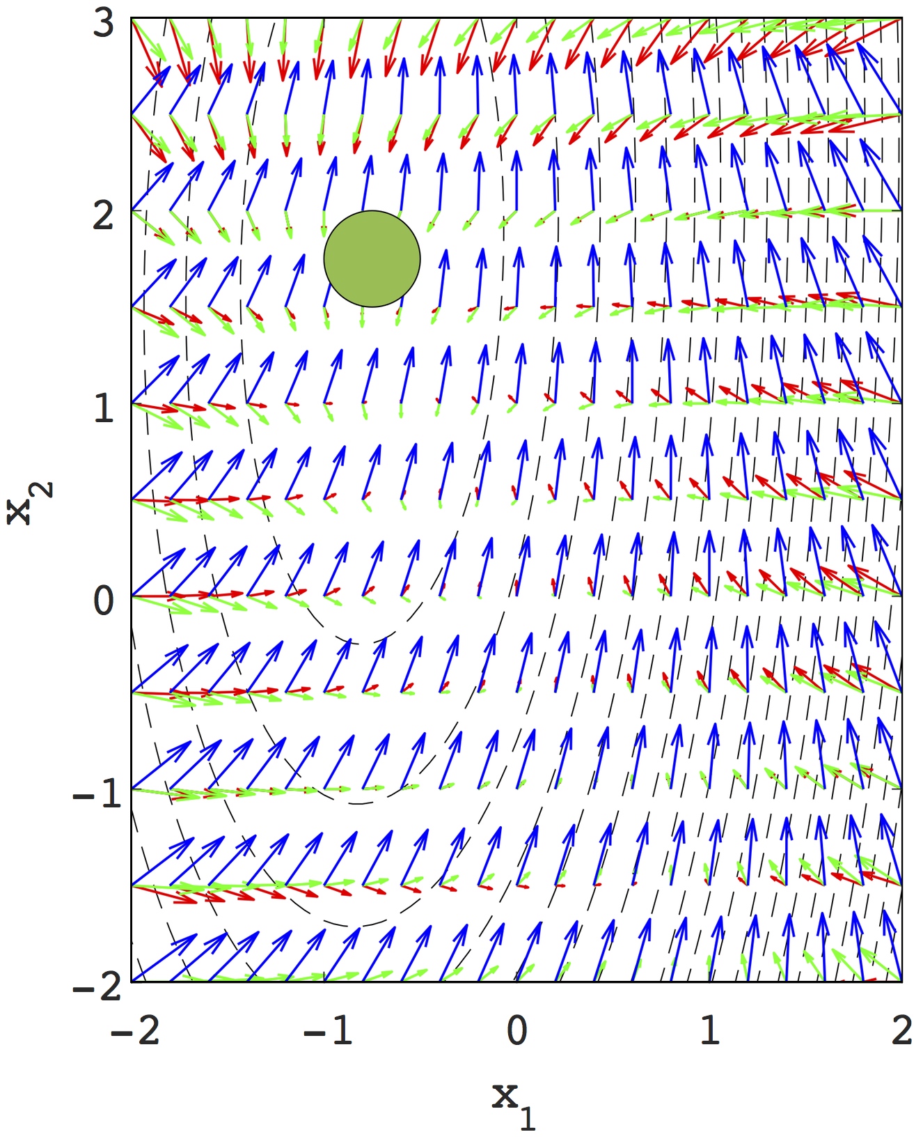
(a)

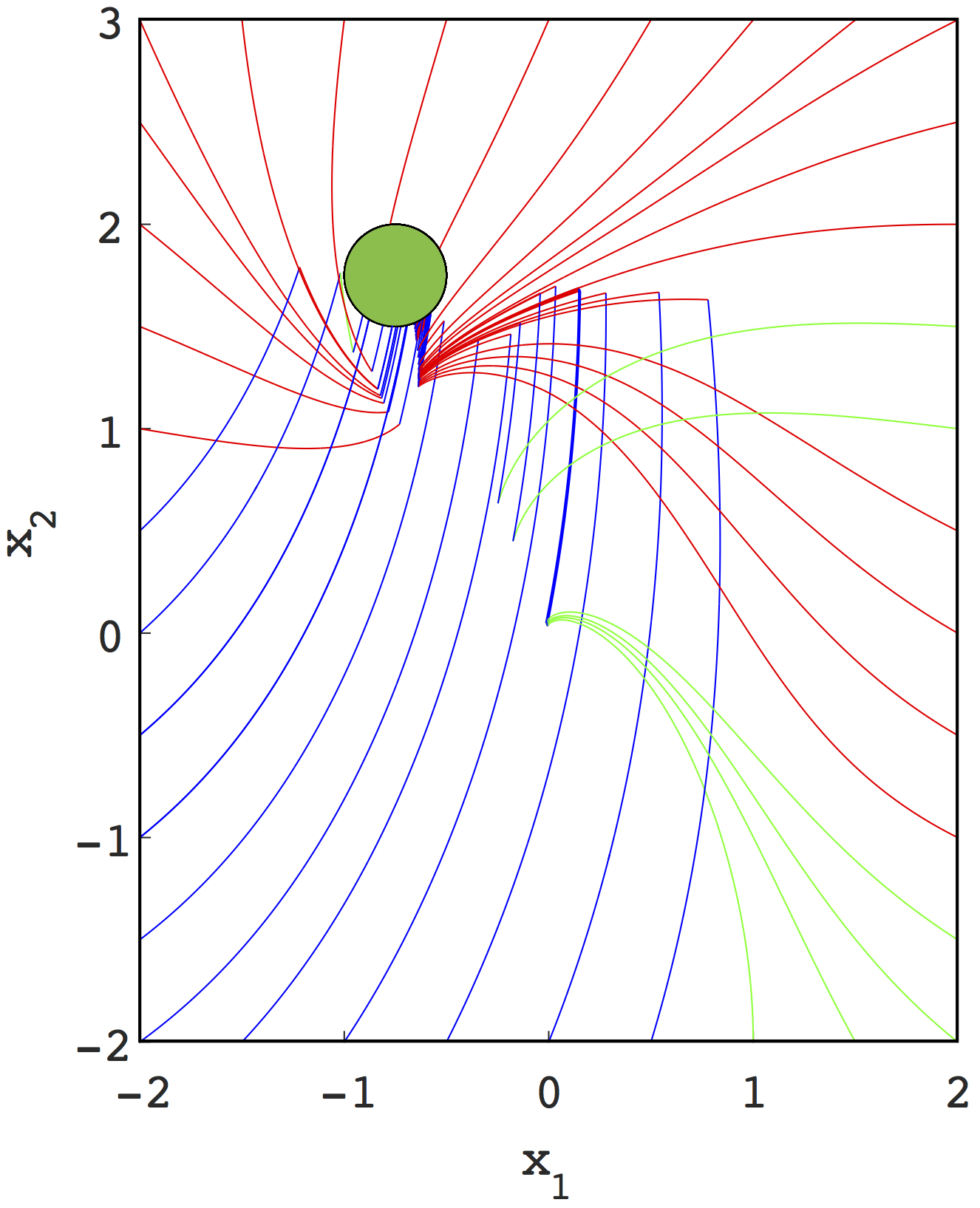
(b)

Figure 1: (a) Region $G$ for Example 1 is shown shaded in the center, and the vector fields for modes $q_{1},q_{2}$ and $q_{3}$ are shown in red, green and blue, respectively. Level-sets of $V$ are shown with black dashed lines. (b) Closed loop trajectories for Example 1 using the controller defined by Eq. (10). The segments shown in colors red, green and blue correspond to the modes $q_{1},q_{2}$ and $q_{3}$, respectively.

We now establish the key result that provides a minimum dwell time guarantee.

Lemma 1.

There exists a $\delta>0$ s.t. for all initial conditions $\mathbf{x}(T)\in S\setminus G$, if $\eta_{q}(\mathbf{x}(T))<-\epsilon$, and if the mode of the system is set to $q$ at time $T$, then

$$(\forall t\in[T,T+\delta])\ (\mathbf{x}(t)\in S\setminus G)\ \implies\ \eta_{q}(\mathbf{x}(t))\leq-\epsilon_{s}\,.$$

Proof.

Let $T+\delta$ be the earliest time instant, where $\eta_{q}(\mathbf{x}(T+\delta))\geq-\epsilon_{s}$ while at the same time

$$(\forall t\in[T,T+\delta])\ q(t)=q,\ \mathbf{x}(t)\in S\setminus G\,.$$

At time $T$, $\eta_{q}(\mathbf{x}(T))<-\epsilon$ and at time $T+\delta$, $\eta_{q}(\mathbf{x}(T+\delta))=-\epsilon_{s}$. Note that $\eta_{q}(\mathbf{x})$ is defined as $\max(\alpha_{1}(\mathbf{x}),\ldots,\alpha_{m}(\mathbf{x}))$ for some smooth functions $\alpha_{1},\ldots,\alpha_{m}$. As a result, Since $S$ is a bounded set, and $p$, $f_{q}$, and $V$ are bounded over $S$, there exists a constant $\Lambda>0$ s.t.

$$(\forall\ \mathbf{x}\in S)\ \accentset{\mbox{\large.}}{\alpha_{i,q}}\leq\Lambda\,.$$ (11)

Therefore, for each $\alpha_{i}$, we have

$$\alpha_{i}(\mathbf{x}(T+\delta)) =\alpha_{i}(\mathbf{x}(T))+\int_{t=T}^{T+\delta}\accentset{\mbox{\large.}}{\alpha_{i,q}}(\mathbf{x}(t))dt\leq\alpha_{i}(\mathbf{x}(T))+\Lambda\delta\,.$$

As a result, we conclude that

$$\eta_{q}(\mathbf{x}(T+\delta)) =\max_{i}\alpha_{i}(\mathbf{x}(T+\delta))=\alpha_{j^{*}}(\mathbf{x}(T+\delta))\leq\alpha_{j^{*}}(\mathbf{x}(T))+\Lambda\delta\leq\eta_{q}(T)+\Lambda\delta\,.$$

Therefore, we can conclude $-\epsilon_{s}<-\epsilon+\Lambda\delta\implies\frac{\epsilon-\epsilon_{s}}{\Lambda}<\delta$ and there exists a fixed $\delta>\frac{\epsilon-\epsilon_{s}}{\Lambda}>0$ s.t.

$$(\forall t\in[T,T+\delta))\ \eta_{q}(\mathbf{x}(t))<-\epsilon_{s}\,.\blacksquare$$

Eq. (10) gives a switching strategy which respects the min-dwell time and as long as $\mathbf{x}(t)\in S$, the controller guarantees $\eta_{q(t)}(\mathbf{x}(t))\leq-\epsilon_{s}$. I.e. for all $j\in J_{q}$, $\accentset{\mbox{\large.}}{V_{q}}(\mathbf{x}(t))\leq-\epsilon_{s}$ and $\accentset{\mbox{\large.}}{p_{S,j,q}}(\mathbf{x}(t))+\lambda p_{S,j}(\mathbf{x}(t))\leq-\epsilon_{s}$.

Theorem 1.

Given nondegenerate  basic  semialgebraic set $S$, a semialgebraic set $G$, and a function $V$ (satisfying Equation (5)), the control strategy defined by Eq. (10) respects the min-dwell time property and guarantees the RWS property defined by $S,G$: $S\implies S\mathcal{U}G$.

Proof.

As discussed, there exists a controller which respects the min-dwell time property. Also, the controller guarantees $\accentset{\mbox{\large.}}{V_{q}}(\mathbf{x})\leq-\epsilon_{s}$ and $(\accentset{\mbox{\large.}}{p_{S,j,q}}(\mathbf{x})+\lambda p_{S,j}(\mathbf{x})\leq-\epsilon_{s}$ (for all $j\in J_{q}$), as long as $\mathbf{x}\in S\setminus G$.

Assume $\mathbf{x}(t)$ is on the boundary of $S$ (and not in $G$) at some time $t$. Because $S$ is assumed to be a nondegenerate basic semialgebraic set, there exists at least one $j$ s.t. $p_{S,j}(\mathbf{x}(t))=0$. If $j\notin J_{q}$, by definition, $\accentset{\mbox{\large.}}{p_{S,j,q}}$ is negative for all states and $p_{S,j,q}$ remains $\leq 0$ as long as mode $q$ is selected. Otherwise ($j\in J_{q}$), we obtain $\accentset{\mbox{\large.}}{p_{S,j,q}}(\mathbf{x}(t))\leq-\epsilon_{s}<0$. Therefore, there exits $\tau_{j}>0$, s.t. $s\in(t,t+\tau_{j})$, we conclude that $p_{S,j,q}(\mathbf{x}(s))<0$. As a result, the trajectory cannot leave the set $S$.

Thus, the trace cannot leave $S$, unless it reaches $G$. Now, we show that the trajectory cannot stay inside $S\setminus G$ forever. By the construction of the controller, we can conclude time diverges (because the controller respects the min-dwell time property) and that $V$ decreases ($\accentset{\mbox{\large.}}{V_{q}}(\mathbf{x}(t))\leq-\epsilon_{s}$). However, the value of $V$ is bounded on bounded set $S\setminus G$. Therefore, $\mathbf{x}$ cannot remain in $S\setminus G$ and the only possible outcome for the trace is to reach $G$. $\blacksquare$

4 RWS for Semialgebraic Safe Set

As Habets et al [7] discussed, control-to-facet problems can be used to build an abstraction. Here, we demonstrate that the method described so far can be integrated in this framework to tackle more complicated problems. First, we briefly explain how the method works. For a more detailed discussion, the reader can refer to [7] or  [12].

First, state space is decomposed into polytopes according to the specifications. Here, we can use basic semialgebraic sets instead of polytopes. Then, for each such a set $u$, we consider an abstract state $\mathcal{A}(u)$. Furthermore, for each of its $n-1$ dimensional facet $F$, a control-to-facet problem is solved. The corresponding problem is to find a control strategy to reach $F$ starting from $u$. If the control-to-facet problem is solved successfully, then for each basic semialgebraic set $v$ with a $n-1$ dimensional facet $F^{\prime}\subseteq F$, an edge from $\mathcal{A}(u)$ to $\mathcal{A}(v)$ (with label/action $F$) is added to the abstraction. Also for each basic semialgebraic set $u$, one can check if $u$ is a control invariant to build self loops. However, for RWS properties, self loops are redundant and we skip them here. After building the abstract system, we use standard techniques to solve the problem for finite systems. If the problem could be solved for the abstract system, then, one can design a controller.

First, for each abstract state $\mathcal{A}(u)$, there is at least one action $F$ that agrees with the winning strategy for the abstract system. Let that action be $\mathcal{F}(\mathcal{A}(u))$. The idea is to implement transition $\mathcal{F}(\mathcal{A}(u))$, using controller $\mathcal{K}_{u,\mathcal{F}(\mathcal{A}(u))}$ for the corresponding control-to-facet problem [7]. Formally, the controller can be defined as follows:

$$\mathcal{K}(q,\mathbf{x})=\begin{cases}\mathcal{K}_{u_{1},\mathcal{F}(\mathcal{A}(u_{1}))}(q,\mathbf{x})\hskip 28.45274pt\mathbf{x}\in u_{1}\\ \vdots\\ \mathcal{K}_{u_{s},\mathcal{F}(\mathcal{A}(u_{s}))}(q,\mathbf{x})\hskip 28.45274pt\mathbf{x}\in u_{s}\,.\end{cases}$$ (12)

When $\mathbf{x}$ belongs to multiple sets, one can break the tie by some ordering, where states in the winning set have priorities. It is worth mentioning that combining these controllers together, does not produce any Zeno behavior as it is guaranteed that each abstract state is visited only once for RWS properties. However, superdense switching is possible as two facets of a polytope can get arbitrarily close.

If one is interested in LTL properties (not just reach-while-stay) or min-dwell time property, one possible solution is to use fat facets, where the target sets are $n$ dimensional goal sets. This extends the domain of the control-to-facet problem to adjacent basic semialgebraic sets as well. Also, it allows the controller to continue using current sub-controller for some minimum time (if min-dwell time requirement is not met), before changing the sub-controller (at the switch time).

Example 5.

Consider again the system from Example 1, with the addition of some obstacles [20]. More precisely, as shown in Fig 2(a), safe set is $S=S_{0}\setminus(O_{1}\cup O_{2})$. First, the safe set is decomposed into four basic semialgebraic sets, which are shown with $R_{0}$ to $R_{3}$ in Fig. 2(a).

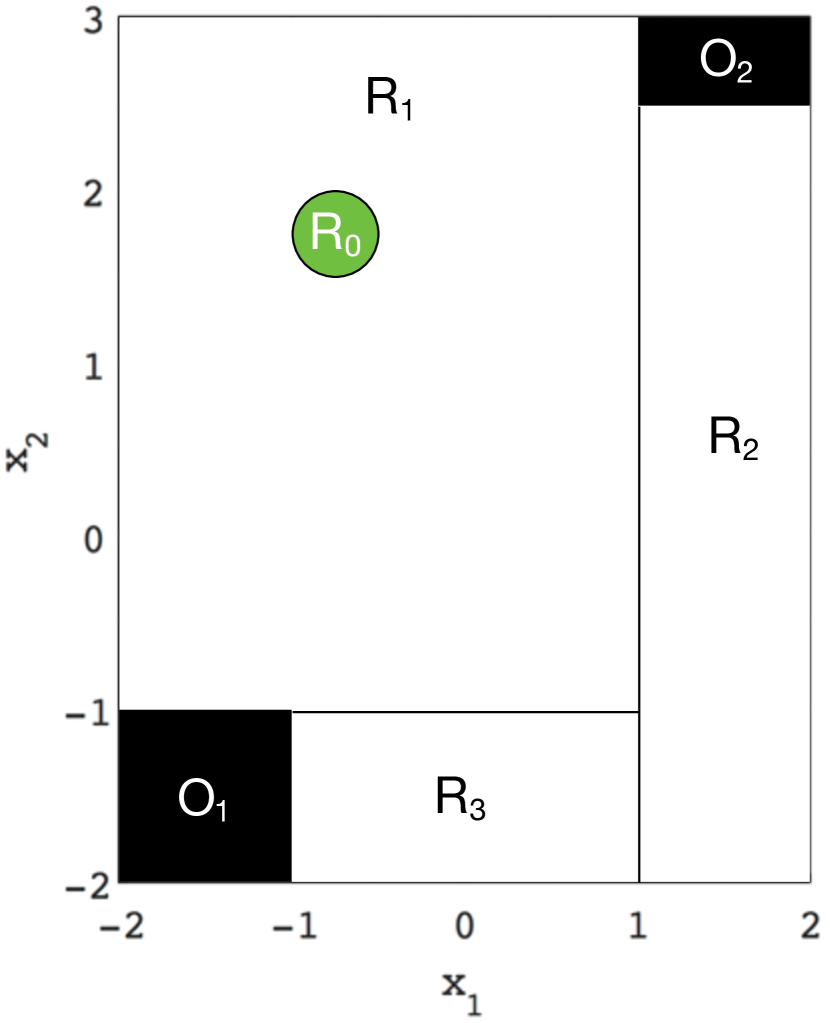
(a)

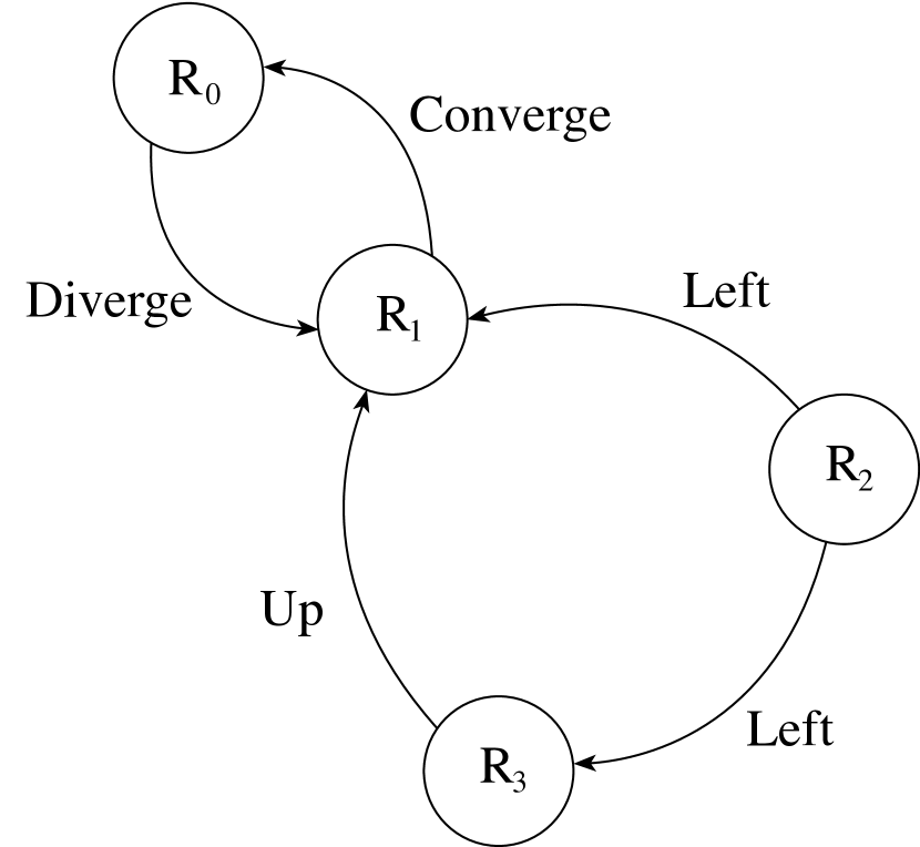
(b)

Figure 2: (a) Schematic view of state decomposition. (b) Finite abstraction for the original problem.

$R_{0}$ is the target set. Next, we build a transition relation between four abstract states, representing four basic semialgebraic sets. This is done by solving seven RWS problems for basic semialgebraic sets. For $R_{1}$ to $R_{0}$, we use a quadratic template for $V$, and for other problems, we use linear template. The abstract system is shown in Fig. 2(b). Next, the problem is solved for the abstract system. The solution to the abstract system is simple: if the state is in $R_{2}$, the controller uses the left facet to reach $R_{1}$ or $R_{3}$. Otherwise, if the state is in $R_{3}$, the controller uses the upper facet to reach $R_{1}$ and finally, if the state is in $R_{1}$, the controller makes sure the state reaches $R_{0}$.

Example 6.

This example is a path planning problem for the unicycle [26]. Projection of safe set on $x$ and $y$ yields a maze. The target set is placed at the right bottom corner of the maze (Fig. 3). Using specification-guided technique, we modeled the system with 53 polyhedra. Each polyhedron is treated as a single state and a transition relation is built by solving 113 control-to-facet problems. Then, the problem is solved over the finite graph. The total computation took 1484 seconds. The figure also shows a single trajectory of the closed loop system.

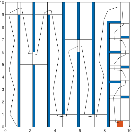
Figure 3: Region $G$ is shown shaded in Orange, and unsafe regions are shown in blue. An execution trace of the car is shown for $x$ and $y$ variables.

Example 7.

This example is similar to Example 6, except for the fact that there is no direct control over the angular velocity. More precisely, only the angular acceleration is controllable and the system would have the following dynamics $\accentset{\mbox{\large.}}{x}=u_{1}\cos(\theta),\,\accentset{\mbox{\large.}}{y}=u_{1}\sin(\theta),\,\accentset{\mbox{\large.}}{\theta}=\omega,\,\accentset{\mbox{\large.}}{\omega}=u_{2}\,.$ Also, we assume $\omega\in[-1,1]$. By changing the coordinates one can use $r=\sqrt{x^{2}+y^{2}}$, $z_{1}=x\cos(\theta)+y\sin(\theta)$ and $z_{2}=y\cos(\theta)-x\sin(\theta)$ to define position and angle of the car(cf. [14] for details). Then, we use the following template $V(x,y,\theta,\omega)=c_{1}r^{2}+c_{2}z_{1}+c_{3}z_{2}\omega+c_{4}\omega^{2}$, where the origin is located just outside of the target facet. Using this template, we find control certificates for all 113 control-to-facet problems in 5296 seconds.

5 Initialized Reach-While-Stay

So far, we discussed uninitialized RWS specifications ($S$ $\implies S\mathcal{U}G$). In these systems, we use boundary of safe set as barrier. However, as pointed out by Lin et al. [15], this may not be the case. Now, we consider the initialized problem for a given initial set $I$ ($I\implies S\mathcal{U}G$). To avoid technical difficulties, we assume that $I\subseteq int(S)$. The solution is to create a composite barrier that is formed by the boundary of $S$ as well as other a priori unknown barrier functions.

Barrier Functions:

We recall that for a control barrier function [30, 37], the following conditions are considered

$$\begin{array}[]{l}\mathbf{x}\in\partial S\implies B(\mathbf{x})>0\\ \mathbf{x}\in I\implies B(\mathbf{x})<0\\ \mathbf{x}\in S\implies\left(B(\mathbf{x})=0\implies(\exists q)\accentset{\mbox{\large.}}{B_{q}}(\mathbf{x})<-\epsilon\right)\,.\end{array}$$ (13)

This ensures that $B(\mathbf{x})=0$ is a barrier and $\partial S$ is unreachable. Eq. (13), combined with the smoothness of $B$ and $f_{q}$ ensures that as soon as the state is sufficiently “close” to the barrier, it is possible to choose a control mode that ensures the local decrease of the $B$.

The condition in Equation (13) can be encoded into the CEGIS framework. However, the presence of the equality $B(\mathbf{x})=0$ poses practical problems. In particular, it requires for each candidate $B_{\mathbf{c}}$, to find a counterexample $\mathbf{x}$ s.t. $B_{\mathbf{c}}(\mathbf{x})\not=0$. Unfortunately, such an assertion is easy to satisfy, resulting in the procedure always exceeding the maximum number of iterations permitted.

Again, we find that the following relaxation of the third condition is particularly effective in our experiments

$$\begin{array}[]{l}\mathbf{x}\in\partial S\ \implies\ B(\mathbf{x})>0\\ \mathbf{x}\in I\ \implies\ B(\mathbf{x})<0\\ \mathbf{x}\in S\implies\bigvee_{q}\left(\begin{array}[]{c}\accentset{\mbox{\large.}}{B}_{q}(\mathbf{x})-\lambda B(\mathbf{x})<-\epsilon\lor\accentset{\mbox{\large.}}{B}_{q}(\mathbf{x})+\lambda B(\mathbf{x})<-\epsilon\end{array}\right)\,,\end{array}$$ (14)

for some constant $\lambda$.

Intuitively, by choosing $\lambda=0$, the condition is similar to that of Lyapunov functions, whereas as $|\lambda|\rightarrow\infty$, the condition gets less conservative and in the limit, it is equivalent to the original condition. In fact, for smaller $|\lambda|$ CEGIS terminates faster, but at the cost of missing potential solutions. On the other hand, using larger $|\lambda|$, is less conservative at the cost of CEGIS timing out. We also note that this formulation is less conservative than the one introduced by Kong et al. [13] as our formulation uses two exponential conditions which only forces decrease of value of $B$ around $B^{*}=\{\mathbf{x}\ |\ B(\mathbf{x})=0\}$.

To solve the RWS in general form, we define a finite set of barriers $\mathcal{B}$ with the following conditions:

$$\begin{array}[]{l}\mathbf{x}\in\partial S\implies\bigvee_{B\in\mathcal{B}}B(\mathbf{x})>0\\ \mathbf{x}\in I\implies\bigwedge_{B\in\mathcal{B}}B(\mathbf{x})<0\,.\end{array}$$ (15)

Also for each mode $q$, $\mathcal{B}_{q}$ is defined as $\mathcal{B}_{q}=\{B\in\mathcal{B}|(\exists\mathbf{x})\accentset{\mbox{\large.}}{B_{q}}(\mathbf{x})>0\}$. Then, existence of a proper mode can be encoded as the following:

$$\begin{array}[]{l}\mathbf{x}\in S\setminus G\implies\left(\begin{array}[]{c}\left(\accentset{\mbox{\large.}}{V_{q}}(\mathbf{x})<-\epsilon\right)\ \land\bigwedge_{B\in\mathcal{B}_{q}}\left(\begin{array}[]{c}\accentset{\mbox{\large.}}{B_{q}}(\mathbf{x})+\lambda B(\mathbf{x})<-\epsilon\lor\\ \accentset{\mbox{\large.}}{B_{q}}(\mathbf{x})-\lambda B(\mathbf{x})<-\epsilon\end{array}\right)\end{array}\right)\,.\end{array}$$ (16)

Theorem 2.

Given nondegenerate  basic  semialgebraic set $S$, semialgebraic sets $I$ and $G$, function $V$, and a non-empty set of functions $\mathcal{B}$ (satisfying Equation (15) and  (16)), there is a control strategy that respects the min-dwell time property and guarantees the RWS property: $I\implies S\mathcal{U}G$.

To simplify these constraints and reduce the number of unknowns, one can use some of $p_{S,i}$’s to fix some of these barriers, which yields conditions similar to the ones used for the uninitialized problem. This trick is demonstrated in the following example.

Example 8.

This example is taken from [17], in which a DC-DC converter is modeled with two variables $i$ and $v$.

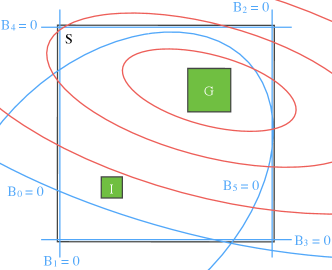
Figure 4: The blue lines are the barriers and the red lines are level-sets of the Lyapunov function.

The system has two modes $q_{1}$ and $q_{2}$, with the following dynamics:

$$q_{1}: \begin{cases}\accentset{\mbox{\large.}}{i}=0.0167i+0.3333\\ \accentset{\mbox{\large.}}{v}=-0.0142v\end{cases}$$

$$q_{2}: \begin{cases}\accentset{\mbox{\large.}}{i}=-0.0183i-0.0663v+0.3333\\ \accentset{\mbox{\large.}}{v}=-0.0711i-0.0142v\,.\end{cases}$$

The safe set is $S:[0.65,1.65]\times[4.95,5.95]$ and the goal set is $G:[1.25,1.45]\times[5.55,5.75]$. We assume initial set to be $I:[0.85,0.95]\times[5.15,5.25]$ (Fig. 4). Then, we use 5 barriers $B_{0},\ldots,B_{4}$. Using boundaries of $S$, we choose $B_{1},\ldots,B_{4}$ as follows:

$$B_{1}= 0.65-i+\epsilon_{b} B_{2}=1.65-i+\epsilon_{b}$$

$$B_{3}= 4.95-v+\epsilon_{b} B_{4}=5.95-v+\epsilon_{b}\,,$$

where $\epsilon_{b}>0$ is small enough that $I\subset int(\bigcap_{i=1}^{4}B_{i})$. In this case, we choose $\epsilon_{b}=0.01$. Notice that such $\epsilon_{b}$ always exists by the definition. Next, we assume $B_{0}=V$ and both have the following template:

$$B_{0}=V:c_{1}(i-1.35)^{2}+c_{2}(i-1.35)(v-5.65)+c_{3}(v-5.65)^{2}-1\,.$$

This template is chosen in a way that $V$ is a quadratic function with minimum value of $-1$ for the point of interest $i=1.35$, $v=5.65$. So far, we used these tricks to reduce the number of unknowns for barriers. However, our method fails to find a certificate. Next, we add one more barrier ($B_{5}$) to the formulation and we use the following template for $B_{5}:c_{4}(i-0.9)^{2}+c_{5}(i-0.9)(v-5.2)+c_{6}(v-5.05)^{2}-1$, which is a quadratic function with minimum value of $-1$ for initial point $i=0.9$, $v=5.2$. This time, we can successfully find a control certificate. The final barriers and level-sets of the Lyapunov function is shown in Fig. 4.

Comparison:

While abstraction based methods can provide a near optimal solution (are relatively complete), these methods can be computationally expensive. On the other hand, our method is a Lyapunov-based method and the solution is not necessarily (relatively) complete. For example, our approach assumes that control certificates with a given form (that is given as input by user) exist . As such, the existence of such certificates is not guaranteed and thus, our approach lacks the general applicability of a fixed-point based synthesis. Also, for initialized problems our method needs an initial set as input, while for the abstraction based methods, maximum controllable region can be obtained without the need for specifying the initial set. However, our method is relatively more scalable thanks to recent development in SMT solvers. Here, for the sake of completeness, we provide a brief comparison with SCOTS toolbox [26] for the examples provided in this article. To compare Example 3, we use fat facet and assume target set has a volume (otherwise, because of time discretization, SCOTS cannot find a solution). More precisely, we use target set $[1,1.2]\times[-1,1]^{3}$ instead of $[1,1]\times[-1,1]^{3}$.

All the experiments are ran on a laptop with Core i7 2.9 GHz CPU and 16GB of RAM. The results are reported in Table 1. We also note that if we use larger values for SCOTS parameters, SCOTS fails to solve these problems (initial set is not a subset of controllable region). Table 1 shows that SCOTS performs much better for Example 5 and  8 for which there are only $2$ state variables. For Example 6, both methods have similar performances. And for Example. 3 and Example.7, which have $4$ state variables, our method is faster.

Table 1: Results of Comparison with SCOTS on examples

Legend: $n$: # state variables, $itr$ : # iterations, Time: total computation time, $\eta$: state discretization step, $\tau$: time step. All timings are in seconds and rounded, TO: timeout ($>10$ hours).

Problem		SCOTS				CEGIS
ID	$n$	$\eta$	$\tau$	$itr$	Time	$\delta$	Time
Ex. 5	2	0.162	0.12	18	0	10-4	3
Ex. 8	2	0.012	1.0	106	1	10-4	39
Ex. 6	3	0.22$\times$0.1	0.3	404	989	10-4	1484
Ex. 3	4	0.03$\times$0.13	0.005	48	304	10-5	3
Ex. 7	4	0.1${}^{2}\times$0.052	0.3	TO		10-4	5296

6 Conclusions

In this paper, given a switched system, we addressed controller synthesis problems for RWS with composite barriers. Specifically, we addressed uninitialized problems which are useful for building an abstraction, as well as initialized problems. For each problem, we provided sufficient conditions in terms of “existence of a control certificate”. Also, we demonstrated that searching for a control certificate can be encoded into constrained problems and solving these problems is computationally feasible. In the future, we wish to investigate how the initialized RWS problems can be extended to be used along fixed-point computation based techniques as it allows more flexible switching strategies.

References

- [1]
- [2] Zvi Artstein (1983): Stabilization with relaxed controls. Nonlinear Analysis: Theory, Methods & Applications 7(11), pp. 1163 – 1173, 10.1016/0362-546X(83)90049-4. Available at http://www.sciencedirect.com/science/article/pii/0362546X83900494.
- [3] Rayna Dimitrova & Rupak Majumdar (2014): Deductive control synthesis for alternating-time logics. In: 2014 International Conference on Embedded Software, EMSOFT 2014, New Delhi, India, October 12-17, 2014, pp. 14:1–14:10, 10.1145/2656045.2656054.
- [4] Sicun Gao, Soonho Kong & Edmund M. Clarke (2013): dReal: An SMT Solver for Nonlinear Theories over the Reals. In: Automated Deduction - CADE-24 - 24th International Conference on Automated Deduction, Lake Placid, NY, USA, June 9-14, 2013. Proceedings, pp. 208–214, 10.1007/978-3-642-38574-2_14. Available at https://doi.org/10.1007/978-3-642-38574-2_14.
- [5] L. El Ghaoui & V. Balakrishnan (1994): Synthesis of fixed-structure controllers via numerical optimization. In: Proceedings of 1994 33rd IEEE Conference on Decision and Control, 3, pp. 2678–2683 vol.3, 10.1109/CDC.1994.411398.
- [6] A. Girard, G. Pola & P. Tabuada (2010): Approximately Bisimilar Symbolic Models for Incrementally Stable Switched Systems. IEEE Transactions on Automatic Control 55(1), pp. 116–126, 10.1109/TAC.2009.2034922.
- [7] L. C. G. J. M. Habets, P. J. Collins & J. H. van Schuppen (2006): Reachability and control synthesis for piecewise-affine hybrid systems on simplices. IEEE Transactions on Automatic Control 51(6), pp. 938–948, 10.1109/TAC.2006.876952.
- [8] L.C.G.J.M. Habets & J.H. van Schuppen (2004): A control problem for affine dynamical systems on a full-dimensional polytope. Automatica 40(1), pp. 21 – 35, 10.1016/j.automatica.2003.08.001. Available at http://www.sciencedirect.com/science/article/pii/S0005109803002620.
- [9] M. K. Helwa & M. E. Broucke (2011): Monotonic reach control on polytopes, pp. 4741–4746. 10.1109/CDC.2011.6160866.
- [10] Z. Huang, Y. Wang, S. Mitra, G. E. Dullerud & S. Chaudhuri (2015): Controller synthesis with inductive proofs for piecewise linear systems: An SMT-based algorithm. In: 2015 54th IEEE Conference on Decision and Control (CDC), pp. 7434–7439, 10.1109/CDC.2015.7403394.
- [11] Manuel Mazo Jr., Anna Davitian & Paulo Tabuada (2010): PESSOA: A Tool for Embedded Controller Synthesis. In: Computer Aided Verification, 22nd International Conference, CAV 2010, Edinburgh, UK, July 15-19, 2010. Proceedings, pp. 566–569, 10.1007/978-3-642-14295-6_49. Available at https://doi.org/10.1007/978-3-642-14295-6_49.
- [12] M. Kloetzer & C. Belta (2008): A Fully Automated Framework for Control of Linear Systems from Temporal Logic Specifications. IEEE Transactions on Automatic Control 53(1), pp. 287–297, 10.1109/TAC.2007.914952.
- [13] Hui Kong, Fei He, Xiaoyu Song, William N. N. Hung & Ming Gu (2013): Exponential-Condition-Based Barrier Certificate Generation for Safety Verification of Hybrid Systems. In: Computer Aided Verification - 25th International Conference, CAV 2013, Saint Petersburg, Russia, July 13-19, 2013. Proceedings, pp. 242–257, 10.1007/978-3-642-39799-8_17. Available at https://doi.org/10.1007/978-3-642-39799-8_17.
- [14] Daniel Liberzon (2012): Switching in systems and control. Springer Science & Business Media, 10.1007/978-1-4612-0017-8.
- [15] Z. Lin & M. E. Broucke (2007): Reachability and control of affine hypersurface systems on polytopes. In: 2007 46th IEEE Conference on Decision and Control, pp. 733–738, 10.1109/CDC.2007.4434805.
- [16] J. Liu, N. Ozay, U. Topcu & R. M. Murray (2013): Synthesis of Reactive Switching Protocols From Temporal Logic Specifications. IEEE Transactions on Automatic Control 58(7), pp. 1771–1785, 10.1109/TAC.2013.2246095.
- [17] Sebti Mouelhi, Antoine Girard & Gregor Gössler (2012): CoSyMA: A Tool for Controller Synthesis Using Multi-scale Abstractions. Research Report RR-8108, INRIA. Available at https://hal.inria.fr/hal-00743982.
- [18] Sebti Mouelhi, Antoine Girard & Gregor Gößler (2013): CoSyMA: a tool for controller synthesis using multi-scale abstractions. In: Proceedings of the 16th international conference on Hybrid systems: computation and control, HSCC 2013, April 8-11, 2013, Philadelphia, PA, USA, pp. 83–88, 10.1145/2461328.2461343.
- [19] Leonardo Mendonça de Moura & Nikolaj Bjørner (2008): Z3: An Efficient SMT Solver. In: Tools and Algorithms for the Construction and Analysis of Systems, 14th International Conference, TACAS 2008, Held as Part of the Joint European Conferences on Theory and Practice of Software, ETAPS 2008, Budapest, Hungary, March 29-April 6, 2008. Proceedings, pp. 337–340, 10.1007/978-3-540-78800-3_24. Available at https://doi.org/10.1007/978-3-540-78800-3_24.
- [20] P. Nilsson & N. Ozay (2014): Incremental synthesis of switching protocols via abstraction refinement. In: 53rd IEEE Conference on Decision and Control, pp. 6246–6253, 10.1109/CDC.2014.7040368.
- [21] N. Ozay, J. Liu, P. Prabhakar & R. M. Murray (2013): Computing augmented finite transition systems to synthesize switching protocols for polynomial switched systems. In: 2013 American Control Conference, pp. 6237–6244, 10.1109/ACC.2013.6580816.
- [22] S. Prajna, A. Papachristodoulou & P. A. Parrilo (2002): Introducing SOSTOOLS: a general purpose sum of squares programming solver. In: Proceedings of the 41st IEEE Conference on Decision and Control, 2002., 1, pp. 741–746 vol.1, 10.1109/CDC.2002.1184594.
- [23] H. Ravanbakhsh & S. Sankaranarayanan (2015): Counter-Example Guided Synthesis of control Lyapunov functions for switched systems. In: 2015 54th IEEE Conference on Decision and Control (CDC), pp. 4232–4239, 10.1109/CDC.2015.7402879.
- [24] Hadi Ravanbakhsh & Sriram Sankaranarayanan (2016): Robust Controller Synthesis of Switched Systems Using Counterexample Guided Framework. In: Proceedings of the 13th International Conference on Embedded Software, EMSOFT ’16, ACM, pp. 8:1–8:10, 10.1145/2968478.2968485.
- [25] Bartek Roszak & Mireille E. Broucke (2006): Necessary and sufficient conditions for reachability on a simplex. Automatica 42(11), pp. 1913 – 1918, 10.1016/j.automatica.2006.06.003. Available at http://www.sciencedirect.com/science/article/pii/S0005109806002445.
- [26] Matthias Rungger & Majid Zamani (2016): SCOTS: A Tool for the Synthesis of Symbolic Controllers. In: Proceedings of the 19th International Conference on Hybrid Systems: Computation and Control, HSCC 2016, Vienna, Austria, April 12-14, 2016, pp. 99–104, 10.1145/2883817.2883834.
- [27] Armando Solar Lezama (2008): Program Synthesis By Sketching. Ph.D. thesis, EECS Department, University of California, Berkeley. Available at http://www2.eecs.berkeley.edu/Pubs/TechRpts/2008/EECS-2008-177.html.
- [28] Eduardo D. Sontag (1989): A ‘universal’ construction of Artstein’s theorem on nonlinear stabilization. Systems & Control Letters 13(2), pp. 117 – 123, 10.1016/0167-6911(89)90028-5. Available at http://www.sciencedirect.com/science/article/pii/0167691189900285.
- [29] Ankur Taly, Sumit Gulwani & Ashish Tiwari (2011): Synthesizing switching logic using constraint solving. STTT 13(6), pp. 519–535, 10.1007/s10009-010-0172-8. Available at https://doi.org/10.1007/s10009-010-0172-8.
- [30] Ankur Taly & Ashish Tiwari (2010): Switching logic synthesis for reachability. In: Proceedings of the 10th International conference on Embedded software, EMSOFT 2010, Scottsdale, Arizona, USA, October 24-29, 2010, pp. 19–28, 10.1145/1879021.1879025.
- [31] Weehong Tan & Andrew Packard (2004): Searching for control Lyapunov functions using sums of squares programming. In: Allerton conference on communication, control and computing, pp. 210–219.
- [32] Y. Tazaki & J. i. Imura (2012): Discrete Abstractions of Nonlinear Systems Based on Error Propagation Analysis. IEEE Transactions on Automatic Control 57(3), pp. 550–564, 10.1109/TAC.2011.2161789.
- [33] Wolfgang Thomas, Thomas Wilke et al. (2002): Automata, logics, and infinite games: a guide to current research. 2500, Springer Science & Business Media, 10.1007/3-540-36387-4.
- [34] Peter Wieland & Frank Allgöwer (2007): CONSTRUCTIVE SAFETY USING CONTROL BARRIER FUNCTIONS. IFAC Proceedings Volumes 40(12), pp. 462 – 467, 10.3182/20070822-3-ZA-2920.00076. Available at http://www.sciencedirect.com/science/article/pii/S1474667016355690. 7th IFAC Symposium on Nonlinear Control Systems.
- [35] T. Wongpiromsarn, U. Topcu & A. Lamperski (2016): Automata Theory Meets Barrier Certificates: Temporal Logic Verification of Nonlinear Systems. IEEE Transactions on Automatic Control 61(11), pp. 3344–3355, 10.1109/TAC.2015.2511722.
- [36] Tichakorn Wongpiromsarn, Ufuk Topcu, Necmiye Ozay, Huan Xu & Richard M. Murray (2011): TuLiP: A Software Toolbox for Receding Horizon Temporal Logic Planning. In: Proceedings of the 14th International Conference on Hybrid Systems: Computation and Control, HSCC ’11, ACM, New York, NY, USA, pp. 313–314, 10.1145/1967701.1967747.
- [37] Xiangru Xu, Paulo Tabuada, Jessy W. Grizzle & Aaron D. Ames (2015): Robustness of Control Barrier Functions for Safety Critical Control**This work is partially supported by the National Science Foundation Grants 1239055, 1239037 and 1239085. IFAC-PapersOnLine 48(27), pp. 54 – 61, 10.1016/j.ifacol.2015.11.152. Available at http://www.sciencedirect.com/science/article/pii/S2405896315024106. Analysis and Design of Hybrid Systems ADHS.
- [38] M. Zamani, G. Pola, M. Mazo & P. Tabuada (2012): Symbolic Models for Nonlinear Control Systems Without Stability Assumptions. IEEE Transactions on Automatic Control 57(7), pp. 1804–1809, 10.1109/TAC.2011.2176409.