Using the Markov Chain Monte Carlo method to study the physical properties GeV-TeV BL Lac objects

Abstract

We fit the spectral energy distributions (SEDs) of 46 GeV - TeV BL Lac objects in the frame of leptonic one-zone synchrotron self-Compton (SSC) model and investigate the physical properties of these objects. We use the Markov Chain Monte Carlo (MCMC) method to obtain the basic parameters, such as magnetic field (B), the break energy of the relativistic electron distribution ($\gamma^{\prime}_{\rm{b}}$) and the electron energy spectral index. Based on the modeling results, we support the following scenarios on GeV-TeV BL Lac objects: (1) Some sources have large Doppler factors, implying other radiation mechanism should be considered. (2) Comparing with FSRQs, GeV-TeV BL Lac objects have weaker magnetic field and larger Doppler factor, which cause the ineffective cooling and shift the SEDs to higher bands. Their jet powers are around $4.0\times 10^{45}~{}\rm{erg\cdot s}^{-1}$, comparing with radiation power, $5.0\times 10^{42}~{}\rm{erg\cdot s}^{-1}$, indicating that only a small fraction of jet power is transformed into the emission power. (3) For some BL Lacs with large Doppler factors, their jet components could have two substructures, e.g., the fast core and the slow sheath. For most GeV-TeV BL Lacs, Kelvin-Helmholtz instabilities are suppressed by their higher magnetic fields, leading few micro-variability or intro-day variability in the optical bands. (4) Combined with a sample of FSRQs, an anti-correlation between the peak luminosity $L_{\rm{pk}}$ and the peak frequency $\nu_{\rm{pk}}$ is obtained, favoring the blazar sequence scenario. In addition, an anti-correlation between the jet power $P_{\rm{jet}}$ and the break Lorentz factor $\gamma_{\rm{b}}$ also supports the blazar sequence.

1 INTRODUCTION

Blazars are the subclasses of radio-lond Active Galactic Nuclei (AGNs), subdivided based on their emission lines: the flat spectrum quasars (FSRQs) have strong broad emission lines while BL Lac objects (BL Lacs) have weak or absent optical emission lines (EW$\leq 5\mbox{\AA}$) (Urry & Padovani, 1999). Their broadband emission is mainly dominated by non-thermal components originated from a relativistic jet aligned with our line of sight (Urry & Padovani, 1999), and shows two humps. The low hump, falling into IR and X-rays, is explained with the relativistic electron synchrotron radiation; the high peak, located at MeV and TeV bands, is explained by the lepton or the hadron models (Böttcher, 2010; Böttcher et al., 2013; Cao & Wang, 2014; Zheng et al., 2016). Blazars often exhibit strong and fast variability across all electromagnetic spectrum. The location of synchrotron peak ($\nu_{\rm{sy}}$) is used to classify blazars as the low-synchrotron-peaked (LSP; $\nu_{\rm{sy}}<$ 10¹⁴Hz), the intermediate-synchrotron-peaked (ISP; 10¹⁴Hz $\leq\nu_{\rm{sy}}\leq$ 10¹⁵Hz, and the high-synchrotron-peaked blazars (HSP; $\nu_{\rm{sy}}>$ 10¹⁵Hz) by Abdo et al. (2010).

BL Lac objects are thought to be “blue” quasars with weak or no external seed photons plus an inefficient accretion disk (Narayan et al., 1997; Blandford & Begelman, 1999), their SEDs suffer less contamination by external photons and give us an opportunity to explore the intrinsic physical properties of emitting region as well as the jet. Comparing with the FSRQs, BL Lacs have lower jet power and inefficient accretion ratio. The SEDs of BL Lacs modeled by a certain radiation mechanism allow us to investigate the physical properties. With a large number of blazars, some authors suggested that the jet comprises a dominant proton component and a small fraction of jet power is radiated if there is one proton per electron (Celotti & Ghisellini, 2008; Yan et al., 2014) , and this assumption was also analyzed by Tanaka et al. (2015).

For the blazar sequence (Fossati et al., 1998; Kubo et al., 1998), it is explained as that the radiative cooling is stronger in more powerful blazar. The blazar sequence is formally expressed as the anti-correlation between the peak luminosity ($L_{\rm pk}$) and the peak frequency of the synchrotron component ($\nu_{\rm pk}$) or the anti-correlation between the jet power $P_{\rm{jet}}$ and the break Lorentz factor $\gamma_{\rm{b}}$. Some authors suggest that the sequence is a result of the selection effect (Padovani et al., 2003; Nieppola et al., 2006; Chen & Bai, 2011; Giommi et al., 2005, 2012). However, other authors propose that the blazar sequence still holds theoretically (Ghisellini et al., 1998; Böttcher & Dermer, 2002; Finke, 2013).

TeV BL Lacs usually show a less amount of optical variability than the LBLs do. A few sources of them have large Doppler factor $\delta_{\rm D}$, which are not consistent with ones by VLBI observations (Piner & Edwards, 2014). A new physical scenario has been proposed to fit their SEDs (Tavecchio & Ghisellini, 2008; Chen, 2017), in which a lower $\delta_{\rm D}$ is needed and supported by observations (Giannios & Metzger, 2011).

The statistical study of physical properties on BL Lacs is needed. Some authors (Zhang et al., 2012; Yan et al., 2014; Inoue & Tanaka, 2016; Ding et al., 2017)) use the samples of TeV-GeV BL Lacs to obtain the physical properties by fitting the SEDs. However, the number of objects in samples is small (Zhang et al. (2012)), and the method to fit the SEDs needs the better error evaluation (Yan et al., 2014; Mankuzhiyil et al., 2011, 2012). In addition, Ding et al. (2017) also use a sample of TeV BL Lacs to investigate the physical properties based on a log-parabolic spectrum of electron energy distributions (EEDs). This type of EEDs could reflect stochastic acceleration in the jet. Considering the impact of the EEDs on the SEDs (Yan et al., 2013; Qin et al., 2018), we use the broken power-law spectrum of EEDs to fit the SEDs of a sample of BL Lacs that contains HBL, IBL and LBL. It is noted that this type of EEDs could be produced in the emitting region and is commonly used to fit the SEDs of blazars.

For BL Lac objects, the simplest model is the homogeneous one-zone SSC model. This model has been considerable successes in reproducing the broadband SEDs of all classes of blazars (Ghisellini & Tavecchio, 2010b; Zhang et al., 2012; Xiong & Zhang, 2014), in which the SEDs with two bumps are assumed to be produced by the synchrotron and the inverse Compton (IC) emissions of ultra-relativistic particles (Finke et al., 2008; Ghisellini & Tavecchio, 2010b). In addition, the high-energy gamma-ray photons are attenuated due to the extragalactic background light (EBL) absorption (Persic et al., 2008). The observed VHE flux in the energy $E_{\rm{\gamma}}$ is given by $f_{\rm{obs}}(E_{\rm{\gamma}})=f_{\rm{int}}(E_{\rm{\gamma}})\times e^{-\rm{\tau}{(E_{\rm{\gamma}},z)}}$, where $f_{\rm{obs}}$ and $f_{\rm{int}}$ are the observed and intrinsic flux respectively, and $\rm{\tau}{(E_{\rm{\gamma}},z)}$ is the optical depth of $E_{\gamma}$ photon which depends on the choice of the EBL template. In the paper, we use the EBL model proposed by (Razzaque et al., 2009) and (Finke et al., 2010) to rebuild the SEDs. We explore the high-dimensional model parameters using the MCMC method in fitting (quasi-) simultaneous multi-band spectra based on one-zone SSC scenario. The MCMC method used here is adapted from the public code “CosmoMC” offered by Lewis & Bridle (2002); Mackay (2003). For details, please refer the papers (Mackay, 2003; Yuan et al., 2011; Yan et al., 2013; Yuan et al., 2016) and a review in Sec. 2.

Throughout this work, we take Hubble constant $H_{0}$ = 70 km$\cdot$s${}^{-1}\cdot$Mpc^-1, $\Omega_{\rm M}$ =0.3, and $\Omega_{\Lambda}$=0.7 to calculate the luminosity distance.

2 MODEL AND STRATEGY

In the SSC scenario, we apply an one-zone spherical blob of the jet filled with the uniform magnetic field $B$, moving with velocity $\beta=\nu/c$ Lorentz factor $\Gamma=(1-\beta^{2})^{-1/2}$ at a small angle ($\theta$) to the line of sight, where $c$ is the speed of light. The SED is produced by both the synchrotron radiation and the SSC process, while the observed SED is strongly enhanced by a relativistic Doppler factor given by $\delta_{\rm D}=[\Gamma(1-{\beta}\rm{cos}\theta)]^{-1}$, where $\delta_{\rm D}\approx\Gamma$ if $\theta\approx 1/\Gamma$.

We assume the size $R^{\prime}_{\rm b}$ of a blob to be calculated by $R^{\prime}_{\rm b}\approx\delta_{\rm D}t_{\rm{v,min}}c(1+z)^{-1}$, where $t_{\rm{v,min}}$ is the minimum variability time-scale. Note that the primes are used for the quantities in the rest frame of the black hole, while the unprimed quantities are defined in the observer frame or the blob’s frame. The electron spectrum is described by a broken power-law distribution with the form

$$N(\gamma^{\prime})=\left\{\begin{array}[]{ll}K^{\prime}_{e}\gamma^{\prime-p_{1}}&\mbox{$\gamma^{\prime}_{\rm{min}}\leq\gamma^{\prime}\leq\gamma^{\prime}_{\rm{b}}$}\\ K^{\prime}_{e}{\gamma^{\prime}_{b}}^{p_{2}-p_{1}}\gamma^{\prime-p_{2}}&\mbox{$\gamma^{\prime}_{\rm{b}}<\gamma^{\prime}\leq\gamma^{\prime}_{\rm{max}}$}\\ \end{array},\right.$$ (1)

where $\gamma^{\prime}_{b}$ is the break Lorentz factor, $p_{1,2}$ is the spectral index below and above $\gamma^{\prime}_{\rm{b}}$, $K^{\prime}_{e}$ is the normalization factor. Note that the magnetic field $B$ is defined in the blob’s frame.

The synchrotron flux ($\nu F_{\nu}$) is given by (Saugé & Henri, 2004; Finke et al., 2008)

$$f_{\rm{\epsilon}}^{\rm{syn}}=\frac{\sqrt{3}\delta_{\rm D}^{4}\epsilon^{\prime}e^{3}B}{4\pi d_{\rm L}^{2}}\int_{1}^{\infty}d\gamma^{\prime}N(\gamma^{\prime})R(x),$$ (2)

where $e$ is the fundamental charge, $h$ is the Planck constant, $d_{\rm{L}}$ is the luminosity distance with the redshift $z$, $\epsilon^{\prime}=[h\nu](1+z)m_{e}c^{2}]/\delta_{\rm D}$ is the dimensionless energy of synchrotron photons, $m_{e}$ and $c$ are the mass of electron and the speed of light. Other quantities in equation (2) are $x=4\pi\varepsilon^{\prime}m_{e}^{2}c^{4}/3eBh\gamma^{\prime 2}$, $R(x)=2x^{2}\{K_{4/3}(x)K_{1/3}(x)-0.6x[K_{4/3}^{2}(x)-K_{1/3}^{2}(x)]\}$, and $K_{\alpha}(x)$ is the modified $\alpha$-order Bessel function, and its numerical integration can be found in Finke et al. (2008).

We use the SSC model described by (Finke et al., 2008)

$$f_{\epsilon_{s}}^{\rm{ssc}}=\frac{9\sigma_{\rm T}\epsilon^{\prime}_{s}}{16\pi R^{\prime}_{b}}\int_{0}^{\infty}d\epsilon_{s}^{\prime}\frac{f_{\epsilon}^{\rm syn}}{\epsilon^{\prime 3}}\int_{\gamma^{\prime}_{\rm{min}}}^{\gamma^{\prime}_{\rm{max}}}d\gamma^{\prime}\frac{N(\gamma^{\prime})}{\gamma^{\prime 2}}F(q,\Gamma_{e}),$$ (3)

where $\sigma_{\rm T}$ is the Thomson cross-section, $\epsilon_{s}^{\prime}=[h\nu_{s}](1+z)m_{e}c^{2}]/\delta_{\rm D}$ is the dimensionless energy of IC scattered photons and the function $F(q,\Gamma_{e})$ is given by

$$F(q,\Gamma_{e})=[2q\rm{ln}q+(1+2q)(1-q)+\frac{1}{2}\frac{(\Gamma_{e}q)^{2}}{(1+\Gamma_{e}q)}(1-q)]\quad$$

$$\quad(\frac{1}{4\gamma^{\prime}}<q<1),$$ (4)

where $q=\frac{\varepsilon^{\prime}/\gamma^{\prime}}{\Gamma_{e}(1-\varepsilon^{\prime}/\gamma^{\prime})}$ and $\Gamma_{e}=4\varepsilon^{\prime}\gamma^{\prime}$. In the GeV-TeV regime, the above function has already considered the KN effect, which makes the IC inefficiency.

As shown above, there are nine parameters in the SSC model, including the size of blob $R^{\prime}_{\rm{b}}$, the magnetic field $B$, the Doppler factor $\delta_{\rm{D}}$, and the electron spectrum ($p_{1},p_{2},\gamma^{\prime}_{\rm{min}},\gamma^{\prime}_{\rm{b}},\gamma^{\prime}_{\rm{max}},K^{\prime}_{\rm{e}}$). $\gamma^{\prime}_{\rm{min}}$ is always poorly constrained by the SED modelling. The $\gamma^{\prime}_{\rm{min}}$ of some sources are getting from Zhang et al. (2012), and are set via the method offered by Tavecchio et al. (2000). For the sources not included in Zhang et al. (2012), we also use the method offered by Tavecchio et al. (2000) to obtain the $\gamma^{\prime}_{\rm{min}}$. In this method, the $\gamma^{\prime}_{\rm{min}}$ is obtained by modeling the radio to X-ray data based on the particle distribution with a power law. If no observational data is available to constrain $\gamma^{\prime}_{\rm{min}}$, we set $\gamma^{\prime}_{\rm{min}}$ as 5.0 based on the pretreatment. From $t_{\rm{v,min}}$, we can get the blob’s size. For the sources without minimum variability, we simply set $t_{\rm v,min}$ as one day (Ghisellini et al., 1998; Fossati et al., 2008; Cao & Wang, 2013). Because the model is not sensitive to $\gamma^{\prime}_{\rm{max}}$, $\gamma^{\prime}_{\rm{max}}=100\gamma^{\prime}_{\rm{b}}$ is adopted.

The MCMC technique is well suitable to search multi-dimensional parameter space and obtains the uncertainties of the model parameters based on the observational data (Yuan et al., 2011; Yan et al., 2014, 2015). According to the Bayes’ Theorem, the posterior probability of a model with a set of parameters (hereafter $\vec{\theta}$) upon the data (hereafter $\cal D$) is given by

$$\cal P(\vec{\theta}\mid D)~{}\propto{\cal L}(D\mid\vec{\theta})\cal P(\vec{\theta}),$$ (5)

where ${-\rm{ln}\cal L}(D\mid\vec{\theta})~{}\propto{\sum\limits_{i=1}^{N}(\frac{f_{\rm i}-f_{\rm{obs}}}{\sigma_{\rm{obs}}})^{2}}$ is the likelihood function, and $f_{\rm i}$ is the model flux in the different band and $N$ is the number of data associated with the band, $f_{\rm{obs}}$ and $\sigma_{\rm{obs}}$ are the flux of observational data and its variance respectively. The MCMC ensures that the probability functions of model parameters can be asymptotically obtained by the number density of samples. Comparing with the least-square fitting method, the MCMC can give the better error evaluation and the confident levels (C.L.) of parameters. Furthermore, for a complex model, the MCMC can obtain the fitting results much faster than the chi-square minimization does.

After calculations, two probability distributions can be obtained. The maximum probability is exactly the same as the best-fit one obtained by minimizing the likelihood. The marginalized probability distributions is the probability distribution of the parameters contained in the subset. It gives the probabilities of various values of the parameters in the subset and reflects the confident levels of parameters. To get the same result as in the best-fit method, the marginalized probability distributions require the large number density of samples to run in the calculation procedure. In the paper, we use the best-fit parameters to rebuild the SEDs and give the confident levels of the parameters in the 68%. It is noted that if the parameters are constrained well, then two types of distributions will have the similar shape and interval.

3 APPLICATIONS

Our sample contains 46 $Fermi$ BL Lacs objects, in which the board-band SEDs cover from radio, optical, X-ray to $\gamma$-ray bands. The different types of blazars are from Roma-BZCAT catalog (Massaro et al., 2010) and TeVCat , which contain 32 HBLs, 10 IBLs and 4 LBLs. In the paper, for some BL Lacs with bad $Fermi$ data (such as only flux upper limits), their (quasi-) simultaneous $Fermi$ data are not used to reproduce the SEDs. Instead, for these objects, we add the GeV gamma-ray data which are from the $Fermi$-LAT 4-year Point Source(3FGL) catalog (Acero et al., 2015). Although these data are not simultaneous with the optical, X-ray and TeV bands, they will give a rough constrain on the SEDs and do not affect our results. It is noted that we do not include the 4-year Point data to fit the objects at the flare stage in our sample. The rest data in many bands are from other instruments such as KAV, $Suzaku$, $Beppo$SAX, $Swift$, H.E.S.S and MAGIC. The simultaneous or quasi-simultaneous SEDs data of BZB J1058+5628, OT 081, PKS 0048-09, PKS 0851+202, 1H 1013+498, BZB J0033-1921 and PG 1246+586 are taken from Giommi et al. (2012). The optical-UV and other band data of PKS 0426-380, 4C 01.28 are gotten from Giommi et al. (2012) and Abdo et al. (2010) respectively. The data of B3 2247+381, 1ES 1215+303, RBS 0413, 1H 0414+009 PKS 0447-439 are obtained from Aleksić et al. (2012a), Aleksić et al. (2012b), Aliu et al. (2012a), Aliu et al. (2012b), and Prandini et al. (2012). The SEDs data of remaining objects are taken from the literatures compiled by Zhang et al. (2012).

Table 1: Model parameters derived in the one-zone SSC model. The mean values and the marginalized 68% confidence intervals (CI) are reported .

Source namea	$z$	$B(0.1G)$	$\gamma^{\prime}_{\rm{min}}$	Log[${\gamma^{\prime}_{\rm{b}}}$]	$\delta_{\rm D}(10)$	Log[K${{}^{\prime}_{e}}$]	$p_{1}$	$p_{2}$	$t_{\rm{var}}^{b}$	Log$\frac{M_{\rm B}}{M_{\hbox{$\odot$}}}$	Refc
[1]	[2]	[3]	[4]	[5]	[6]	[7]	[8]	[9]	[10]	[11]	[12]
1ES0229+200	0.140	0.010	5.00	6.16	6.09	53.36	2.02	2.62	24.0	9.2	1
(68% CI)	-	0.010 -  0.024	-	5.99 -  6.25	4.79 -  6.02	53.19 - 53.55	2.00 -  2.09	2.29 -  3.10	-	-	-
1ES0347-121	0.185	0.016	100.00	5.30	7.94	51.43	1.68	2.92	12.01	8.7	1
(68% CI)	-	0.016 -  0.027	-	5.15 -  5.35	6.79 -  8.00	50.58 - 52.14	1.51 -  1.84	2.84 -  2.99	-	-	-
1ES0806+524	0.138	0.377	5.00	4.91	2.44	54.87	2.45	4.07	24.0	8.9	2
(68% CI)	-	0.335 -  0.766	-	4.70 -  4.90	1.83 -  2.58	53.38 - 55.00	2.12 -  2.44	3.83 -  4.21	-	-	-
1ES1011+496	0.212	0.559	5.00	5.11	2.83	52.30	1.81	4.22	24.0	8.3	-
(68% CI)	-	0.267 -  0.865	-	5.05 -  5.24	2.45 -  3.56	52.07 - 52.68	1.77 -  1.88	4.14 -  4.43	-	-	-
1ES1101-232	0.186	0.030	5.00	5.58	7.99	52.07	1.87	3.56	12.01	0.0	-
(68% CI)	-	0.030 -  0.039	-	5.47 -  5.61	7.35 -  8.00	51.47 - 52.34	1.75 -  1.93	3.47 -  3.62	-	-	-
1ES1101-232 f	0.186	17.420	5.00	4.98	0.51	54.30	2.41	4.56	12.01	0.0	-
(68% CI)	-	12.888 - 70.174	-	4.68 -  4.97	0.23 -  0.62	50.83 - 54.13	1.61 -  2.38	3.57 -  4.45	-	-	-
1ES1215+303	0.130	0.100	100.00	4.31	3.54	53.18	1.85	3.57	24.0	8.5	3
(68% CI)	-	0.100 -  0.140	-	4.22 -  4.37	3.12 -  3.51	53.03 - 53.37	1.80 -  1.91	3.53 -  3.62	-	-	-
1ES1218+30.4	0.184	0.174	100.00	4.74	4.33	48.41	1.00	3.60	12.01	8.6	1
(68% CI)	-	0.136 -  0.309	-	4.68 -  4.80	3.59 -  4.64	48.47 - 49.14	1.00 -  1.17	3.53 -  3.72	-	-	-
1ES1959+650	0.047	0.689	5.00	5.51	2.84	53.85	2.46	4.33	10.01	8.1	1
(68% CI)	-	0.461 -  0.878	-	5.46 -  5.59	2.60 -  3.30	53.75 - 53.99	2.44 -  2.48	4.19 -  4.50	-	-	-
1ES2344+514	0.044	0.650	100.00	4.84	1.34	51.74	1.86	3.64	12.02	8.8	1
(68% CI)	-	0.638 -  1.991	-	4.64 -  4.93	0.79 -  1.36	48.81 - 53.68	1.17 -  2.30	3.56 -  3.73	-	-	-
1ES2344+514 f	0.044	0.022	100.00	6.30	3.47	54.86	2.37	4.07	12.02	8.8	1
(68% CI)	-	0.019 -  0.286	-	5.71 -  6.23	1.47 -  2.54	54.23 - 54.75	2.32 -  2.40	2.94 -  5.00	-	-	-
1H0414+009	0.287	0.101	100.00	5.01	5.42	53.68	2.10	3.79	24.0	0.0	-
(68% CI)	-	0.100 -  0.117	-	4.96 -  5.03	5.13 -  5.44	53.31 - 53.98	2.02 -  2.17	3.75 -  3.84	-	-	-
1H1013+498	0.212	3.261	100.00	4.59	1.44	54.01	2.24	3.82	24.0	0.0	-
(68% CI)	-	2.682 -  4.492	-	4.54 -  4.62	1.30 -  1.52	53.94 - 54.13	2.22 -  2.29	3.71 -  3.91	-	-	-
3C66A	0.444	0.385	170.00	4.60	4.48	52.91	1.79	5.07	12.01	8.6	3
(68% CI)	-	0.328 -  0.475	-	4.56 -  4.62	4.11 -  4.80	52.36 - 53.20	1.66 -  1.87	5.01 -  5.13	-	-	-
B32247+381	0.119	0.310	100.00	5.07	2.34	52.98	2.05	4.01	24.0	0.0	-
(68% CI)	-	0.208 -  0.491	-	5.02 -  5.17	1.99 -  2.65	52.86 - 53.20	2.01 -  2.12	3.86 -  4.31	-	-	-
BZBJ0033-1921	0.610	0.101	100.00	4.27	5.42	50.02	1.02	3.34	24.0	0.0	-
(68% CI)	-	0.100 -  0.342	-	4.08 -  4.25	3.77 -  5.29	50.16 - 52.04	1.00 -  1.53	3.31 -  3.35	-	-	-
BZBJ1058+5628	0.143	1.642	100.00	4.08	1.43	54.18	2.25	3.68	24.0	8.7	3
(68% CI)	-	2.755 - 12.155	-	3.72 -  3.99	0.71 -  1.20	51.67 - 54.21	1.62 -  2.30	3.61 -  3.71	-	-	-
H1426+428	0.129	0.101	200.00	5.47	1.26	48.56	1.00	2.86	24.0	9.1	1
(68% CI)	-	0.100 -  0.174	-	5.51 -  5.82	0.79 -  1.13	48.63 - 49.37	1.00 -  1.17	2.78 -  2.95	-	-	-
H2356-309	0.165	0.014	5.00	5.79	5.65	54.94	2.33	3.39	24.0	8.6	1
(68% CI)	-	0.017 -  0.065	-	5.53 -  5.75	3.44 -  5.30	54.43 - 54.89	2.27 -  2.35	3.31 -  3.46	-	-	-
MRK421	0.030	0.546	20.00	4.84	3.83	50.24	1.67	4.05	3.04	8.3	1
(68% CI)	-	0.507 -  0.641	-	4.80 -  4.85	3.62 -  3.94	50.18 - 50.29	1.66 -  1.68	4.01 -  4.08	-	-	-
MRK421 f	0.030	0.116	20.00	5.07	8.00	49.95	1.57	3.50	3.04	8.3	1
(68% CI)	-	0.114 -  0.134	-	5.04 -  5.11	7.54 -  8.00	49.90 - 50.05	1.56 -  1.59	3.44 -  3.55	-	-	-
MRK501	0.034	0.495	200.00	5.40	1.83	55.00	2.61	3.99	12.05	9.2	1
(68% CI)	-	0.331 -  0.724	-	5.31 -  5.48	1.57 -  2.13	54.70 - 55.26	2.54 -  2.66	3.89 -  4.12	-	-	-
MRK501 f	0.034	1.238	5.00	5.64	1.94	48.57	1.48	2.71	1.06	9.2	1
(68% CI)	-	1.085 -  1.428	-	5.61 -  5.67	1.85 -  2.03	48.36 - 48.78	1.44 -  1.53	2.67 -  2.75	-	-	-
Mkn180	0.045	0.432	100.00	4.87	1.35	51.69	1.80	3.62	24.07	8.2	2
(68% CI)	-	0.218 -  5.271	-	4.57 -  4.84	0.42 -  1.26	50.25 - 52.75	1.44 -  2.02	3.50 -  3.68	-	-	-
PG1553+113	0.360	0.101	100.00	4.73	7.76	53.02	1.83	3.97	24.0	8.6	3
(68% CI)	-	0.100 -  0.128	-	4.67 -  4.76	7.07 -  7.70	52.36 - 53.42	1.68 -  1.93	3.94 -  4.00	-	-	-
PKS0447-439	0.107	0.762	100.00	4.70	2.06	55.23	2.49	4.36	24.0	8.8	3
(68% CI)	-	0.616 -  0.906	-	4.63 -  4.76	1.90 -  2.24	54.77 - 55.53	2.38 -  2.56	4.23 -  4.49	-	-	-
PKS1424+240	0.160	0.811	100.00	4.52	3.72	54.99	2.33	5.56	24.08	0.0	-
(68% CI)	-	0.677 -  0.938	-	4.48 -  4.54	3.52 -  3.95	54.62 - 55.21	2.24 -  2.38	5.34 -  5.73	-	-	-
PKS2005-489	0.071	0.115	200.00	4.39	8.00	54.19	2.37	3.20	10.01	8.1	5
(68% CI)	-	0.116 -  0.139	-	4.34 -  4.40	7.46 -  8.00	53.88 - 54.48	2.30 -  2.45	3.17 -  3.23	-	-	-
PKS2155-304	0.116	0.407	400.00	4.43	8.00	51.31	1.81	4.06	2.010	8.7	6
(68% CI)	-	0.397 -  0.430	-	4.39 -  4.47	7.90 -  8.00	50.69 - 51.72	1.66 -  1.92	4.02 -  4.10	-	-	-
PKS2155-304 f	0.116	0.183	200.00	4.95	7.65	54.37	2.37	4.02	2.010	8.7	6
(68% CI)	-	0.183 -  0.423	-	4.63 -  5.05	5.39 -  8.00	51.97 - 54.97	1.80 -  2.50	3.90 -  4.25	-	-	-
RBS0413	0.190	0.104	100.00	5.18	3.19	53.75	2.14	3.42	24.0	8.0	1
(68% CI)	-	0.100 -  0.225	-	4.98 -  5.24	2.44 -  3.09	52.54 - 54.26	1.89 -  2.27	3.29 -  3.53	-	-	-

Table 1. Continue–

Source namea	$z$	$B(0.1G)$	$\gamma^{\prime}_{\rm{min}}$	Log[${\gamma^{\prime}_{\rm{b}}}$]	$\delta_{\rm D}(10)$	Log[K${{}^{\prime}_{e}}$]	$p_{1}$	$p_{2}$	$t_{\rm{var}}^{b}$	Log$\frac{M_{\rm B}}{M_{\hbox{$\odot$}}}$	Refc
[1]	[2]	[3]	[4]	[5]	[6]	[7]	[8]	[9]	[10]	[11]	[12]
RGBJ0152+017	0.080	0.180	5.00	5.04	1.77	56.16	2.70	3.27	24.0	0.0	-
(68% CI)	-	0.101 -  2.434	-	4.54 -  5.18	0.52 -  1.50	51.53 - 55.35	1.70 -  2.56	3.07 -  3.27	-	-	-
RGBJ0710+591	0.125	0.118	800.00	4.99	3.32	54.83	2.46	2.37	24.0	8.3	1
(68% CI)	-	0.100 -  0.700	-	4.82 -  5.00	1.85 -  3.14	54.03 - 54.72	2.31 -  2.47	2.36 -  2.45	-	-	-
S50716+714	0.300	0.393	100.00	3.90	9.97	52.03	1.78	3.91	3.09	8.6	7
(68% CI)	-	0.368 -  0.655	-	3.80 -  3.89	8.31 - 10.00	50.04 - 52.44	1.24 -  1.90	3.88 -  3.93	-	-	-
S50716+714 f	0.300	0.115	100.00	4.24	9.50	52.14	1.68	3.91	3.09	8.6	7
(68% CI)	-	0.100 -  0.678	-	3.96 -  4.22	4.58 -  9.07	50.03 - 52.32	1.00 -  1.73	3.83 -  3.94	-	-	-
PKS0851+202	0.306	1.481	100.00	3.49	2.41	54.10	1.87	5.16	24.0	8.7	3
(68% CI)	-	1.467 -  1.505	-	3.49 -  3.50	2.38 -  2.43	54.08 - 54.12	1.86 -  1.88	5.13 -  5.18	-	-	-
PKS0048-09	0.634	0.207	100.00	3.96	5.16	54.44	1.98	3.74	24.0	0.0	-
(68% CI)	-	0.165 -  0.269	-	3.85 -  4.03	4.63 -  5.72	54.06 - 54.71	1.84 -  2.08	3.70 -  3.78	-	-	-
PG1246+586	0.847	0.080	100.00	4.36	7.62	53.14	1.72	4.00	24.0	0.0	-
(68% CI)	-	0.079 -  0.162	-	4.26 -  4.37	6.09 -  8.00	53.12 - 53.24	1.72 -  1.77	3.97 -  4.03	-	-	-
BLLacertae	0.069	1.556	50.00	3.43	2.82	52.09	1.78	4.00	3.03	8.2	1
(68% CI)	-	1.395 -  1.734	-	3.41 -  3.45	2.71 -  2.94	51.99 - 52.16	1.74 -  1.82	3.96 -  4.03	-	-	-
BLLacertae f	0.069	2.265	50.00	3.68	2.02	53.59	2.33	3.51	3.03	8.2	1
(68% CI)	-	0.821 - 25.789	-	3.51 -  4.54	1.05 -  2.13	53.57 - 54.59	2.34 -  3.00	3.28 -  3.99	-	-	-
Wcom	0.102	0.128	200.00	4.43	3.73	53.42	2.01	3.66	12.011	7.4	4
(68% CI)	-	0.115 -  0.198	-	4.38 -  4.51	3.26 -  3.86	53.34 - 53.67	1.98 -  2.10	3.62 -  3.79	-	-	-
Wcom f	0.102	0.440	200.00	4.18	2.06	53.61	2.00	3.50	12.011	7.4	4
(68% CI)	-	0.101 -  0.709	-	4.14 -  4.29	1.68 -  2.94	53.18 - 53.89	1.88 -  2.08	3.46 -  3.56	-	-	-
PKS0426-380	1.110	0.004	100.00	3.25	12.00	53.25	1.00	2.90	24.0	8.6	3
(68% CI)	-	0.004 -  0.005	-	3.22 -  3.30	11.95 - 12.00	53.22 - 53.33	1.00 -  1.03	2.87 -  2.96	-	-	-
4C01.28	0.890	0.116	100.00	3.96	6.21	55.90	2.27	4.82	24.0	0.0	-
(68% CI)	-	0.103 -  0.132	-	3.91 -  4.03	5.72 -  6.56	55.70 - 56.21	2.20 -  2.39	4.52 -  5.05	-	-	-
OT081	0.322	0.073	100.00	4.12	4.61	55.07	2.05	5.37	24.0	8.7	3
(68% CI)	-	0.071 -  0.077	-	4.10 -  4.14	4.53 -  4.62	55.05 - 55.14	2.05 -  2.08	5.11 -  5.54	-	-	-
PKS1717+177	0.137	0.101	100.00	4.68	1.53	55.73	2.37	4.72	24.0	8.5	3
(68% CI)	-	0.100 -  0.110	-	4.65 -  4.75	1.48 -  1.53	55.70 - 55.79	2.36 -  2.39	4.60 -  5.57	-	-	-

a: The $``\rm f"$ represents the high stage of object. b: The minimum variability timescales refer to the following references: (1)Zhang et al. (2012); (2)Acciari et al. (2011); (3)Ravasio et al. (2002); (4)Błażejowski et al. (2005); (5)Anderhub et al. (2009a); (6)Tavecchio et al. (2001); (7)Albert et al. (2006); (8)Acciari et al. (2010); (9)Foschini et al. (2006); (10)Aharonian et al. (2009); (11)Acciari et al. (2009) c: The black hole mass refer to the following references: (1)Woo & Urry (2002); (2)Wu et al. (2002); (3)Ghisellini et al. (2010a); (4)Liang & Liu (2003); (5)Wagner (2008); (6)Aharonian et al. (2009); (7)Anderhub et al. (2009b)

4 RESULTS AND DISCUSSION

We have studied the sample that contains 39 GeV-TeV $Fermi$ BL Lacs , in which 7 sources have the flare states. As demonstrated above, we use a simple SSC model to reproduce the SEDs, in which the parameters are listed in Table 1 and the SEDs are shown in the figures of the appendix. From the figures, for 5 HBLs, such as 1ES 1011+496, 1H 0414+009, BZBJ 0033-1921, BZBJ 1058+5628, MRK 421, 1 IBL S5 0716-714 and 1 LBL OT 081, the simple SSC model does not well fit their SEDs. For some objects, such as PG 1246+586 and PKS 0851+202, their VHE ($\geq$ 100 GeV) have a upward trend, and their origin is still debated. In addition, for these objects with 4-year $Fermi$-LAT data, such as H 2356-309 and PKS 2005-489, their SEDs in GeV band are not well fitted.

4.1 Distributions of Model Parameters

From the Table 1 and Fig. 1, the redshift distribution of GeV-TeV BL Lacs extends from 0.03 to 1.11, the derived black hole masses are around $10^{8}M_{\hbox{$\odot$}}$. It is found that the values of $B$ are more extreme than that given by Ghisellini et al. (2010a) and Zhang et al. (2012), and most of them are around 0.01, except for 1ES 1101-232 in the high stage, because its emission mechanism is still on debate. It is implied that lower magnetic field could lead to ineffective cooling and $\gamma^{\prime}_{b}$ will shift to higher value causing hard Gamma rays. The Doppler factor $\delta_{\rm D}$ for most sources is clustered at 11.6, however, a few are larger than 50 and even reach to 100. In addition, the Doppler distribution seems to have a double-hump, which could be caused by the limited numbers of the sample or the unsuitable SSC model, and we will further discuss this problem later. It is noted that the objects in our sample are all low redshift objects.

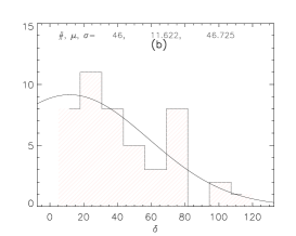
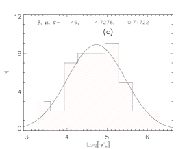
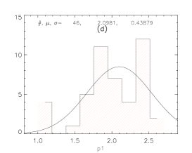
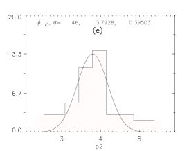
Figure 1: (a) and (b) The distributions of the magnetic field B and the beaming factor $\delta_{\rm D}$. (c) The distribution of the break Lorentz factor $\gamma_{b}$. (d) and (e) The spectral index $p_{1}$ and $p_{2}$. The Gauss function is used to fit the modeling parameter. “#”, “$\mu$” and “$\sigma$” represent the number of the BL Lac object, the mean and the standard deviation of the modeling parameter respectively.

4.2 Properties of Jet

We calculate the jet power and the radiative power using the parameters obtained from our model. The jet power can be estimated by $P_{\rm{jet}}=\pi R^{\prime 2}_{\rm{b}}\Gamma^{2}c(U^{\prime}_{\rm{e}}+U^{\prime}_{\rm{p}}+U^{\prime}_{\rm{B}})$, where the emitting electron $U^{\prime}_{\rm{e}}$, the cold proton $U^{\prime}_{\rm{p}}$ and the magnetic field $U^{\prime}_{\rm{B}}$ are given by

$$U^{\prime}_{\rm{e}}=m_{\rm{e}}c^{2}\int{n(\gamma)\gamma}{d\gamma},$$ (6)

$$U^{\prime}_{\rm{p}}=m_{\rm{p}}c^{2}\int{n(\gamma)}{d\gamma},$$ (7)

$$U^{\prime}_{\rm{B}}=\frac{B^{2}}{8\pi},$$ (8)

where $n(\gamma$)=${N(\gamma)}/{\frac{4\pi R^{\prime 3}_{\rm b}}{3}}$ obtained by the assumption of one proton per emitting electron. For the radiative power $P_{\rm{r}}$, it can be estimated by the total non-thermal luminosity as

$$P_{\rm{r}}=L^{\prime}\Gamma^{2}\approx L\frac{\Gamma^{2}}{\delta^{4}},$$ (9)

where $L$ is obtained by the SED fits. The results are reported in Table 2 and Fig. 2. It is found that the values of $LogP_{\rm{r}}$,$LogP_{\rm B}$, $LogP_{\rm e}$, $LogP_{\rm p}$ and $LogP_{\rm{jet}}$ are clustered at 42.7, 42.6, 44.8, 45.5 and 45.6 respectively. The distribution of radiative power shows a bimodal and could be caused by the limited numbers of the sample. In our sample, we can see from the table: (1)there is $P_{e}>P_{B}$, showing that the jets are particle-dominated; (2) there is $P_{r}\sim P_{B}$, indicating that the Poynting flux accounts for the observed radiation; (3) there are $P_{r}<P_{e}$ and $P_{p}\sim P_{jet}$, suggesting that an additional energy reservoir of protons is needed to accelerate electrons (Tanaka et al. (2015)). Most sources have the equipartition parameter $U^{\prime}_{\rm e}/U^{\prime}_{\rm B}$ to be $1-10^{3}$, but some sources have $U^{\prime}_{\rm e}/U^{\prime}_{\rm B}$ to be larger than several thousands, and even to $10^{6}$, implying that one zone SSC model could be unsuitable.

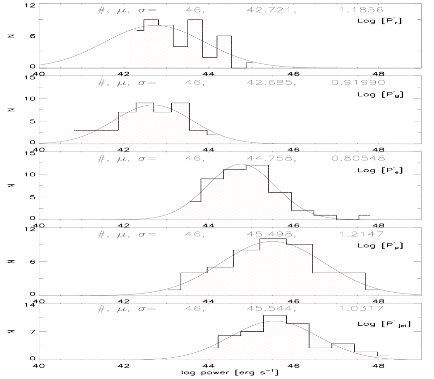
Figure 2: The distributions of radiative power ($P^{\prime}_{\rm{r}}$), Poynting flux ($P^{\prime}_{\rm{B}}$), electron ($P^{\prime}_{\rm{e}}$), proton ($P^{\prime}_{\rm{p}}$) and total jet power ($P^{\prime}_{\rm{jet}}$). Symbols are the same as in Fig.1.

Table 2: The ratios of the energy densities of relativistic electrons to magnetic field in the emitting regions, the jet powers in the forms of bulk motion of electrons, protons and Poynting flux and the radiative powers .

Source namea	$U^{\prime}_{\rm e}/U^{\prime}_{\rm B}$	Log $P_{\rm r}$	Log $P_{\rm B}$	Log $P_{\rm e}$	Log $P_{\rm p}$	Log $P_{\rm{jet}}$
[1]	[2]	[3]	[4]	[5]	[6]	[7]
1ES0229+200	4991.4	42.9	41.4	45.1	47.0	47.0
1ES0347-121	1555.6	42.3	41.7	44.8	44.6	45.0
1ES0806+524	144.6	42.9	43.0	45.2	47.1	47.1
1ES1011+496	6.3	43.9	43.5	44.3	45.3	45.4
1ES1101-232	337.4	42.4	42.2	44.7	45.9	45.9
1ES1101-232 f	23.2	45.2	43.0	44.3	46.4	46.4
1ES1215+303	267.0	42.7	42.5	44.9	45.3	45.4
1ES1218+30.4	34.2	42.9	42.7	44.2	43.4	44.3
1ES1959+650	30.5	42.7	43.1	44.6	46.6	46.6
1ES2344+514	33.5	42.6	41.9	43.4	43.7	43.9
1ES2344+514 f	44187.8	42.2	40.6	45.3	46.0	46.0
1H0414+009	61.7	43.0	43.1	44.9	45.4	45.5
1H1013+498	1.7	44.3	43.9	44.1	44.8	44.9
3C66A	130.6	44.5	43.3	45.4	45.5	45.7
B32247+381	15.4	42.8	42.8	44.0	44.4	44.5
BLLacertae	70.2	42.9	42.7	44.6	45.3	45.4
BLLacertae f	114.0	43.2	42.5	44.5	45.6	45.6
BZBJ0033-1921	193.4	43.5	42.9	45.2	44.7	45.3
BZBJ1058+5628	7.9	43.5	43.3	44.2	44.9	45.0
H1426+428	4485.9	43.7	40.7	44.4	42.7	44.4
H2356-309	14317.8	42.1	41.6	45.7	47.4	47.4
MRK421	21.2	42.5	42.4	43.7	44.2	44.3
MRK421 f	93.5	42.4	42.3	44.3	44.4	44.6
MRK501	107.1	42.6	42.2	44.2	44.8	44.9
MRK501 f	394.6	43.8	41.0	43.5	43.5	43.8
Mkn180	13.4	42.4	42.2	43.3	43.4	43.7
PG1553+113	42.8	43.6	43.7	45.3	45.6	45.8
PKS0447-439	26.5	43.5	43.3	44.8	45.6	45.6
PKS1424+240	7.2	44.2	44.4	45.2	46.0	46.0
PKS2005-489	36.8	42.4	43.3	44.9	45.3	45.5
PKS2155-304	37.6	42.8	43.0	44.6	44.4	44.8
PKS2155-304 f	3724.8	43.7	42.2	45.8	46.2	46.3
RBS0413	188.8	42.7	42.3	44.6	45.1	45.2
RGBJ0152+017	8161.4	42.6	41.8	45.7	47.6	47.6
RGBJ0710+591	56.1	43.0	42.5	44.3	44.1	44.5
S50716+714	53.5	43.2	43.5	45.3	45.7	45.8
S50716+714 f	2678.4	43.5	42.4	45.8	46.0	46.2
PKS0851+202	22.4	44.5	44.0	45.4	46.0	46.1
PKS0048-09	331.8	44.2	43.5	46.0	46.5	46.6
PG1246+586	468.7	43.8	43.2	45.9	46.1	46.3
Wcom	466.7	42.7	42.2	44.9	45.1	45.3
Wcom f	375.4	43.7	42.3	44.8	45.1	45.3
PKS0426-380	5394623	44.3	41.3	48.1	48.3	48.5
4C01.28	3603.1	44.2	43.1	46.7	47.4	47.5
OT081	5157.9	43.7	42.5	46.3	46.8	46.9
PKS1717+177	27975.9	43.4	41.0	45.5	46.2	46.3

As mentioned in Section 4.1, a few sources have large $\delta_{\rm D}$, which are not consistent with ones by VLBI observations (e.g., Piner & Edwards (2014)). Several authors proposed the jet model with spine-sheath (Tavecchio & Ghisellini, 2008) or the decelerating-jet model (Georganopoulos & Kazanas, 2003) to reduce the extreme $\delta_{\rm D}$ (and bulk Lorentz factor). For Swift J1644+57 and Swift J2058+05 (Mimica et al., 2015), the rapid X-ray variability could be originated from the internal jet, similar to the blazar geometry of normal AGNs (Bloom et al., 2011). However, the radio flux increased gradually over several months could be caused by the shock interaction between the fast core and the dense external gas surrounding the SMBH (Giannios & Metzger, 2011), which is similar to GRB afterglows, indicating that the relativistic jet may contain a fast core and slow sheath. In addition, HBLs usually show weak micro-variability or intro-day variability in the optical bands, supporting the model offered by Gaur et al. (2012) that the Kelvin-Helmholtz instability (Romero et al., 1999) is suppressed when $B>B_{\rm c}$, where $B_{\rm c}$ is the critical value of the axial magnetic fields in sub-parsec to parsec scale jets which is given by (Romero, 1995)

$$B_{\rm c}=\frac{\sqrt{4\pi nm_{\rm e}c^{2}(\Gamma^{2}-1)}}{\Gamma},$$ (10)

where $n$ and $m_{\rm e}$ are the electron density and rest mass respectively, and $\Gamma$ is the bulk Lorentz factor. If $\Gamma\gg 1$, then $B_{\rm c}\sim\sqrt{4\pi nm_{\rm e}c^{2}}$. Although we use simple SSC model to reproduce the SEDs, as demonstrated above, but one-zone jet model could be unreasonable for sources with extreme bulk Lorentz, and the spine-sheath jet model is approved. In our sample, the larger $\delta_{\rm D}$ corresponds the lower $B$. This also well known for extreme blazar such as 1ES 0229+200 and 1ES 0347-121(e.g., Tanaka et al. (2014)), so there should be $B<B_{\rm{real}}$ for two component model. We roughly take $B/B_{\rm c}$ to check the instability shown in Fig. 3. It is found that the Kelvin-Helmholtz instability is suppressed for most GeV-TeV BL Lac objects, which show few micro-variability in the optical bands. BL Lacs with $B/B_{\rm c}<$ 1 contain all LBLs and some HBLs, they may involve the IC radiation process from weak extra field.

Figure 3: Kelvin-Helmholtz instabilities in sub-parsec to parsec scale jets will be suppressed if the magnetic field $B$ exceeds the critical value $B_{c}$. The vertical line represents the value of $B/B_{c}$ =1.0.

4.3 Relativistic electron distributions and Accretion rates

For electron distributions, $p_{\rm 1}$ and $p_{\rm 2}$ are clustered at 2.1 and 3.7 respectively. This result favors that $N^{\prime}(\gamma^{\prime})\propto\gamma^{\prime-2}$ or $p_{\rm 1}\sim 2$ for $\gamma^{\prime}<\gamma^{\prime}_{\rm b}$, which is expected in the slow-cooling regime (Finke, 2013). In addition, one can find that for BZB J0033-1921 and PKS 0426-380, their $p_{\rm 1}$ are smaller than 1.3 and deviate from the standard picture that $N^{\prime}(\gamma^{\prime})\sim\gamma^{\prime-q}$ below $\gamma^{\prime}_{\rm b}$ in slow-cooling regime if electrons are injected with $\sim\gamma^{-q}$. However, standard shock acceleration theories predict that q $\sim$ 2 or $N^{\prime}(\gamma^{\prime})\sim\gamma^{\prime-2}$ in the fast-cooling regime. Some authors introduced new acceleration mechanisms, such as magnetic reconnection (Guo et al., 2014, 2016) and collisionless shocks (Asano & Terasawa, 2015), or the KN effect on the SSC (Bošnjak & Daigne, 2014) and IC (Yan et al., 2016) emissions to obtain a hard electron distribution, but for these objects with the low magnetization ($\sigma\leq 1$, $\sigma=\frac{B}{\sqrt{4\pi nm_{\rm e}c^{2}}}$), like 1ES 2344-514 and PKS 0426-380, the magnetic reconnection is inefficient in a matter dominated flow.

Figure 4: Distributions of accretion rates in Eddington units. The Gauss fit result is plotted on the picture. Symbols are the same as in Fig.1.

Fig. 4 shows the accretion rates $\dot{M}$ in Eddington unit, in which we set $\dot{M}=\frac{P_{\rm{jet}}}{c^{2}}$ (Ghisellini & Tavecchio, 2008). It is found that $Log[\dot{M}/\dot{M_{\rm Edd}}]$ is clustered at -2.07, and only 5 sources have accretion rates larger than -1 which is a ^′′divide^′′ value between FSRQs and BL Lacs (Ghisellini et al., 2010a). It is interesting to note that PKS0426-380 and OT081 (LBL) with high accretion rates could show LBL to be different from IBL/HBL and need complex emission mechanism such as IC(Tanaka et al., 2013).

4.4 The blazar sequence

In the paper, we constructed a large sample of GeV-TeV BL Lacs plus FSRQs obtained from Kang et al. (2014) to test the blazar sequence. $\nu_{\rm{pk}}$ is obtained by

$$\nu_{\rm{pk}}=\frac{4}{3}\gamma^{\prime}_{b}\nu_{\rm{L}}\frac{\delta_{\rm D}}{1+z},$$ (11)

where $\nu_{\rm L}$ is the Larmor frequency.

The relation of $\nu_{\rm{pk}}-L_{\rm{pk}}$ for the sample is plotted in Fig. 5. It is found that FSRQs are located at the top-left region, and BL Lacs cover at the down-right region. Our sample also contains some objects in the flare stage. Using the correlation analysis, we find that there are a strong anti-correlations between $\nu_{\rm{pk}}$ and $L_{\rm{pk}}$ in our sample. The sample sources with low stage could have stronger anti-correlations than that for the sources with flare stage. In addition, we also plot the relation of $\gamma^{\prime}_{\rm b}-P^{\prime}_{\rm{jet}}$ based on BL Lacs, shown on the right panel of Fig. 5.

Figure 5: The top panel: the peak luminosity $L_{\rm{pk}}$ as a function of the peak frequency $\nu_{\rm{pk}}$. The correlation coefficients of the best-fit line for the sample containing low (line A) and high states (line B), are -0.47 and -0.42 respectively. The solid black squares and circles are BL Lacs in low stage and high stage, respectively. The open triangle represents the FSRQs. The bottom panel: the power $P^{\prime}_{\rm{jet}}$ of the jet as a function of the break Lorentz factor $\gamma^{\prime}_{\rm b}$, where the correlation coefficient of the best-fit line is - 0.116. The solid black circles are BL Lacs.

Based on the correlations of $\nu_{\rm{pk}}-L_{\rm{pk}}$ and $\gamma^{\prime}_{\rm b}-P^{\prime}_{\rm{jet}}$, we support the blazar sequence, in which the radiation energy density causes a particle energy distribution to be a break at low energies (Fossati et al., 1998; Ghisellini & Tavecchio, 2008; Fan et al., 2016). Despite of the anti-correlation presented in Fig.5, the flare could shift $\nu_{\rm b}$ to the high bands. In addition, for several BL Lacs, their types do not match what given in the literature, and their SEDs may fail to be reproduced by the simply one-zone SSC model. Furthermore, we also find that for some BL Lacs, such as 1ES 1101+496, their peak luminosity in the low hump decrease even they are in the high state, the main reason is that the flare does not happen in the optical to the X-ray bands.

5 SUMMARY

We have reproduced the SEDs of 46 GeV-TeV BL Lacs upon one-zone SSC model using the MCMC technology, then we use the best-fitting model parameters to analyze the jet powers, the accretion rates, and their correlations. Based on our sample, we also test the blazar sequence and the proper structure of the jet.

Firstly, the MCMC technology enable us to reproduce GeV-TeV BL Lacs SEDs based on the simultaneous or quasi-simultaneous observation data in a large range of the parameter space, avoiding visual identification. One zone SSC model can well produce the observed SEDs, however, for some objects such as LBLs, other radiation mechanism should be considered. In addition, some distributions show bimodal phenomenon, which reflect the limited number of objects or the emission mechanism should be revisited. Secondly, GeV-TeV BL Lacs are old blue quasars, and they have weak magnetic field and large Doppler factor, which cause ineffective cooling and shift the SEDs to higher bands. Their jet powers are around $4.0\times 10^{45}\rm{erg\cdot s}^{-1}$, comparing with the radiation power, $5.0\times 10^{42}\rm{erg\cdot s}^{-1}$, indicating that only a small fraction of the jet power is transformed into the emission power. Thirdly, we argue that for some BL Lacs with large Dopplers, their jet components could have two substructures, e.g., the fast core and the slow sheath. For most GeV-TeV BL Lacs, the Kelvin-Helmholtz instability is suppressed by the higher magnetic fields, leading few micro-variability or intro-day variability in the optical bands. Finally, $L_{\rm{pk}}-\nu_{\rm{pk}}$ and $\gamma_{\rm b}-P_{\rm{jet}}$ have the anti-correlations, favoring the blazar sequence.

6 appendix: Parameters Distributions And Spectral Energy Distributions

Fig. 6. Left panels: the distributions of the model parameters, where the dotted lines show the maximum likelihood distributions, the solid lines show the marginalized probability distributions. Right panels: the SEDs of GeV-TeV objects.

Fig. 6.— continued

Fig. 6.— continued

Fig. 6.— continued

Fig. 6.— continued

Fig. 6.— continued

Fig. 6.— continued

Fig. 6.— continued

Fig. 6.— continued

Fig. 6.— continued

Fig. 6.— continued

Fig. 6.— continued

References

- Abdo et al. (2009) Abdo, A. A., et al. 2009, ApJ, 707, 1310
- Abdo et al. (2010) Abdo, A. A., Ackermann, M., Agudo, I., et al. 2010, ApJ, 716, 30
- Abdo et al. (2011a) Abdo, A. A. et al. 2011a, ApJ, 736, 131
- Abdo et al. (2011b) Abdo, A. A. et al. 2011b, ApJ, 727, 129
- Abdo et al. (2011c) Abdo, A. A., Ackermann, M., Ajello, M., et al. 2011c, ApJ, 726, 43
- Acciari et al. (2009) Acciari, V., et al. 2009, ApJL, 690, L126
- Acciari et al. (2010) Acciari, V. A., et al. 2010, ApJL, 715, L49
- Acciari et al. (2011) Acciari, V. A., Aliu, E., Arlen, T., et al. 2011, ApJ, 738, 169
- Acero et al. (2015) Acero, F., Ackermann, M., Ajello, M., et al. 2015, ApJS, 218, 23
- Aharonian et al. (2009) Aharonian, F., et al. 2009, A&A, 502, 749
- Albert et al. (2006) Albert, J., et al. 2006, ApJL, 648, L105
- Aleksić et al. (2012a) Aleksić, J., Alvarez, E. A., Antonelli, L. A., et al. 2012, A&A, 539, A118
- Aleksić et al. (2012b) Aleksić, J., Alvarez, E. A., Antonelli, L. A., et al. 2012, A&A, 544, A142
- Aliu et al. (2012a) Aliu, E., Archambault, S., Arlen, T., et al. 2012, ApJ, 750, 94
- Aliu et al. (2012b) Aliu, E., Archambault, S., Arlen, T., et al. 2012, ApJ, 755, 118
- Anderhub et al. (2009a) Anderhub, H., et al. 2009a, ApJ, 705, 1624
- Anderhub et al. (2009b) Anderhub, H., et al. 2009b, ApJL, 704, L129
- Asano & Terasawa (2015) Asano, K., & Terasawa, T. 2015, MNRAS, 454, 2242
- Blandford & Begelman (1999) Blandford, R. D., & Begelman, M. C. 1999, MNRAS, 303, L1
- Błażejowski et al. (2005) Blazejowski, M., et al. 2005, ApJ, 630, 130
- Bloom et al. (2011) Bloom, J. S., Giannios, D., Metzger, B. D., et al. 2011, Science, 333, 203
- Böttcher & Dermer (2002) Böttcher, M., & Dermer, C. D. 2002, ApJ, 564, 86
- Böttcher (2010) Böttcher, M. 2010, arXiv:1006.5048
- Böttcher et al. (2013) Böttcher, M., Reimer, A., Sweeney, K., & Prakash, A. 2013, ApJ, 768, 54
- Bošnjak & Daigne (2014) Bošnjak, Ž., & Daigne, F. 2014, A&A, 568, A45
- Cao & Wang (2013) Cao, G., & Wang, J.-C. 2013, MNRAS, 436, 2170
- Cao & Wang (2014) Cao, G., & Wang, J. 2014, ApJ, 783, 108
- Celotti & Ghisellini (2008) Celotti, A., & Ghisellini, G. 2008, MNRAS, 385, 283
- Chen & Bai (2011) Chen, L., & Bai, J. M. 2011, ApJ, 735, 108
- Chen (2017) Chen, L. 2017, ApJ, 842, 129
- Contestant (2007) Costamante, L. 2007, Ap&SS, 309, 487
- Dermer & Schlickeiser (1993) Dermer, C. D. & Schlickeiser, R. 1993, ApJ, 416, 458
- Dermer & Schlickeiser (2002) Dermer, C. D. & Schlickeiser, R. 2002, ApJ, 575, 667
- Ding et al. (2017) Ding, N., Zhang, X., Xiong, D. R., & Zhang, H. J. 2017, MNRAS, 464, 599
- Fan et al. (2016) Fan, X.-L., Bai, J.-M., & Mao, J. 2016, arXiv:1607.05000
- Finke et al. (2008) Finke, J. D., Dermer, C. D., Böttcher, M. 2008, ApJ, 686, 181-194
- Finke et al. (2010) Finke, J. D., Razzaque, S., & Dermer, C. D. 2010, ApJ, 712, 238
- Finke (2013) Finke, J. D. 2013, ApJ, 763, 134
- Fossati et al. (1998) Fossati, G., Maraschi, L., Celotti, A., Comastri, A., & Ghisellini, G. 1998, MNRAS, 299, 433
- Foschini et al. (2006) Foschini, L., Tagliaferri, G., Pian, E., et al. 2006, Ap&SS, 455, 871
- Fossati et al. (2008) Fossati, G. et al. 2008, ApJ, 677, 906
- Gaur et al. (2012) Gaur, H., Gupta, A. C., Strigachev, A., et al. 2012, MNRAS, 420, 3147
- Georganopoulos & Kazanas (2003) Georganopoulos, M., & Kazanas, D. 2003, ApJL, 594, L2
- Ghisellini et al. (1985) Ghisellini, G., Maraschi, L., Treves, A. 1985, Ap&SS, 146, 204
- Ghisellini & Madau et al. (1996) Ghisellini, G. & Madau, L. 1996, MNRAS, 208, 67
- Ghisellini et al. (1998) Ghisellini, G., Celotti, A., Fossati, G., Maraschi, L., & Comastri, A. 1998, MNRAS, 301, 451
- Ghisellini et al. (2005) Ghisellini G., Tavecchio F., Chiaberge M., 2005, Ap&SS, 432, 401
- Ghisellini & Tavecchio (2008) Ghisellini, G., Tavecchio, F., 2008, MNRAS, 386, L28
- Ghisellini et al. (2010a) Ghisellini, G., Tavecchio, F., Foschini, L., et al. 2010, MNRAS, 402, 497
- Ghisellini & Tavecchio (2010b) Ghisellini, G., & Tavecchio, F. 2010, MNRAS, 409, L79
- Giannios & Metzger (2011) Giannios, D., & Metzger, B. D. 2011, MNRAS, 416, 2102
- Giommi et al. (2005) Giommi, P., Piranomonte, S., Perri, M., & Padovani, P. 2005, A&A, 434, 385
- Giommi et al. (2012) Giommi, P., Padovani, P., Polenta, G., et al. 2012, MNRAS, 420, 2899
- Guo et al. (2014) Guo, F., Li, H., Daughton, W., & Liu, Y.-H. 2014, Physical Review Letters, 113, 155005
- Guo et al. (2016) Guo, F., Li, X., Li, H., et al. 2016, ApJL, 818, L9
- Inoue & Tanaka (2016) Inoue, Y., & Tanaka, Y. T. 2016, ApJ, 828, 13
- Kang et al. (2014) Kang, S.-J., Chen, L., & Wu, Q. 2014, ApJS, 215, 5
- Kubo et al. (1998) Kubo, H., Takahashi, T., Madejski, G., et al. 1998, ApJ, 504, 693
- Lewis & Bridle (2002) Lewis, A., & Bridle, S. 2002, Phys. Rev., 66, 103511
- Liang & Liu (2003) Liang, E. W., & Liu, H. T. 2003, MNRAS, 340, 632
- Mackay (2003) Mackay, D. J. C. 2003, Information Theory, Inference and Learning Algorithms, UK: Cambridge University Press, 640
- Mankuzhiyil et al. (2011) Mankuzhiyil, N., Ansoldi, S., Persic, M., & Tavecchio, F. 2011, ApJ, 733, 14
- Mankuzhiyil et al. (2012) Mankuzhiyil, N., Ansoldi, S., Persic, M., et al. 2012, ApJ, 753, 154
- Massaro et al. (2010) Massaro, E., Giommi, P., Leto, C., et al. 2010, arXiv:1006.0922
- Mimica et al. (2015) Mimica, P., Giannios, D., Metzger, B. D., & Aloy, M. A. 2015, MNRAS, 450, 2824
- Narayan et al. (1997) Narayan, R., Garcia, M. R., & McClintock, J. E. 1997, ApJL, 478, L79
- Nieppola et al. (2006) Nieppola, E., Tornikoski, M., & Valtaoja, E. 2006, A&A, 445, 441
- Padovani et al. (2003) Padovani, P., Perlman, E. S., Landt, H., Giommi, P., & Perri, M. 2003, ApJ, 588, 128
- Persic et al. (2008) Persic, M., De Angelis, A., Longo, F., & Tavani, M. 2008, International Cosmic Ray Conference, 3, 917
- Piner & Edwards (2014) Piner, B. G., & Edwards, P. G. 2014, ApJ, 797, 25
- Prandini et al. (2012) Prandini, E., Bonnoli, G., & Tavecchio, F. 2012, A&A, 543, A111
- Qin et al. (2018) Qin, L., Wang, J., Yan, D., et al. 2018, MNRAS, 473, 3755
- Ravasio et al. (2002) Ravasio, M., et al. 2002, A&A, 383, 763
- Razzaque et al. (2009) Razzaque, S., Dermer, C. D., & Finke, J. D. 2009, ApJ, 697, 483
- Romero (1995) Romero, G. E. 1995, Ap&SS, 234, 49
- Romero et al. (1999) Romero, G. E., Cellone, S. A., & Combi, J. A. 1999, A&AS, 135, 477
- Rügamer et al. (2011) Rügamer, S., Angelakis, E., Bastieri, D., et al. 2011, arXiv:1110.6341
- Saugé & Henri (2004) Saugé, L., & Henri, G. 2004, ApJ, 616, 136
- Tanaka et al. (2013) Tanaka, Y. T., Cheung, C. C., Inoue, Y., et al. 2013, ApJ, 777, L18
- Tanaka et al. (2014) Tanaka, Y. T., Stawarz, Ł., Finke, J., et al. 2014, ApJ, 787, 155
- Tanaka et al. (2015) Tanaka, Y. T., Doi, A., Inoue, Y., et al. 2015, ApJL, 799, L18
- Tavecchio et al. (1998) Tavecchio, F., Maraschi, L., Ghisellini, G. 1998, ApJ, 509, 608
- Tavecchio et al. (2001) Tavecchio, F. et al. 2001, ApJ, 554, 725
- Tavecchio et al. (2000) Tavecchio, F., Maraschi, L., Sambruna, R. M., & Urry, C. M. 2000, ApJ, 544, L23
- Tavecchio & Ghisellini (2008) Tavecchio, F., & Ghisellini, G. 2008, MNRAS, 385, L98
- Urry & Padovani (1999) Urry, C. M. & Padovani, P. 1999, ApJ, 11, 159
- Wagner (2008) Wagner, R. M. 2008, MNRAS, 385, 119
- Werner et al. (2016) Werner, G. R., Uzdensky, D. A., Cerutti, B., Nalewajko, K., & Begelman, M. C. 2016, ApJL, 816, L8
- Woo & Urry (2002) Woo, J.-H., & Urry, C. M. 2002, ApJ, 579, 530
- Wu et al. (2002) Wu, X.-B., Liu, F. K., & Zhang, T. Z. 2002, A&A, 389, 742
- Xiong & Zhang (2014) Xiong, D. R., & Zhang, X. 2014, MNRAS, 441, 3375
- Yan et al. (2013) Yan, D., Zhang, L., Yuan, Q., Fan, Z., & Zeng, H. 2013, ApJ, 765, 122
- Yan et al. (2014) Yan, D., Zeng, H., & Zhang, L. 2014, MNRAS, 439, 2933
- Yan et al. (2015) Yan, D., Zhang, L., & Zhang, S.-N. 2015, MNRAS, 454, 1310
- Yan et al. (2016) Yan, D., Zhang, L., & Zhang, S.-N. 2016, MNRAS, 459, 3175
- Yuan et al. (2011) Yuan, Q., Liu, S., Fan, Z., Bi, X., & Fryer, C. L. 2011, ApJ, 735, 120
- Yuan et al. (2016) Yuan, Z., Wang, J., Zhou, M., & Mao, J. 2016, ApJ, 820, 65
- Zhang et al. (2012) Zhang, J., Liang, E. W., Zhang, S. N., & Bai, J. M. 2012, ApJ, 752, 157
- Zheng et al. (2016) Zheng, Y. G., Yang, C. Y., & Kang, S. J. 2016, A&A, 585, A8