An Approach for Accelerating Incompressible Turbulent Flow Simulations Based on Simultaneous Modelling of Multiple Ensembles

Abstract

The present paper deals with the problem of improving the efficiency of large scale turbulent flow simulations. The high-fidelity methods for modelling turbulent flows become available for a wider range of applications thanks to the constant growth of the supercomputers performance, however, they are still unattainable for lots of real-life problems. The key shortcoming of these methods is related to the need of simulating a long time integration interval to collect reliable statistics, while the time integration process is inherently sequential.

The novel approach with modelling of multiple flow states is discussed in the paper. The suggested numerical procedure allows to parallelize the integration in time by the cost of additional computations. Multiple realizations of the same turbulent flow are performed simultaneously. This allows to use more efficient implementations of numerical methods for solving systems of linear algebraic equations with multiple right-hand sides, operating with blocks of vectors. The simple theoretical estimate for the expected simulation speedup, accounting the penalty of additional computations and the linear solver performance improvement, is presented. The two problems of modelling turbulent flows in a plain channel and in a channel with a matrix of wall-mounted cubes are used to demonstrate the correctness of the proposed estimates and efficiency of the suggested approach as a whole. The simulation speedup by a factor of 2 is shown.

1 Introduction

The modelling of turbulent flows is one of the typical applications for high performance computing (HPC) systems. The accurate eddy-resolving simulations of turbulent flows are characterized by huge computational grids and long time integration intervals, making them extremely time-consuming to solve. Despite the constant growth of the computational power of HPC systems, the use of high-fidelity methods is still unattainable for lots of real-life applications. This motivates the researchers to develop new computational algorithms and adapt the known algorithms to the modern HPC systems.

The high-order time integration schemes are typically used to increase the accuracy of turbulent flow simulations with eddy-resolving methods. The 3-th or 4-th order explicit or semi-implicit Runge-Kutta schemes (e.g., [1, 2, 3]) or 2-nd order Adams-Bashforth/Crank-Nicolson schemes [4, 5, 6, 7] are among the widely used ones for time integration of incompressible flows. In these schemes, the preliminary velocity distributions are obtained from the Navier-Stokes equations, and the continuity equation, transformed to the elliptic pressure Poisson equation, is used to enforce a divergence-free velocity field. Commonly, the solution of elliptic equations and corresponding systems of linear algebraic equations (SLAEs) is a complicated and challenging problem. The time to compute this stage can take up to 95% of the overall simulation time.

For a limited number of problems with regular computational domains, solved on structured grids, the direct methods for solving SLAEs can be used (e.g., [8, 9]). Otherwise, the iterative methods are the good candidates to solve SLAEs with matrices of the general form. The multigrid methods [10] or Krylov subspace methods (e.g., BiCGStab [11, 12, 13], GMRES [14]) with multigrid preconditioners are the popular ones to solve the corresponding systems. The advantages of these methods are related to their robustness and excellent scalability potential [15]. Mathematically, these methods consist of a combination of linear operations with dense vectors, ${\bf z}=a{\bf x}+b{\bf y}$, scalar products, $a=({\bf x},{\bf y})$, and sparse matrix-dense vector multiplications (SpMV), ${\bf y}={\bf Ax}$. While the linear operations with dense vectors and scalar products are easily vectorized by compilers and acceptable performance is achieved, the performance of SpMV operations is dramatically lower. The sparse matrix-vector multiplication is a memory-bound operation with extremely low arithmetic intensity. The real performance of linear algebra algorithms with sparse matrices of the general form does not exceed several percent of the peak performance [16, 17, 18]. The optimizations of operations with sparse matrices, which are related to both optimization of matrix storage formats and implementation aspects are a topic of continuous research for many years (e.g., [19, 20, 21, 22]).

The performance of SpMV-like operations can be significantly improved if applied to a block of dense vectors simultaneously (generalized SpMV, GSpMV), ${\bf Y}={\bf AX}$, where $\bf X$ and $\bf Y$ are dense matrices [16, 23, 24, 25]. Generally, the performance gain of GSpMV operation with $m$ vectors compared to $m$ successive SpMV operations is achieved due to two main factors: (i) the reduction of the memory traffic to load the matrix $\bf{A}$ from the memory (the matrix is read only once) and (ii) vectorization improvement for GSpMV operation.

Despite the significant performance advantage of matrix-vector operations with blocks of vectors over the single-vector operations, the GSpMV-like operations are rarely used in real computations. This fact is a consequence of the numerical algorithms design: most of them operate with single vectors only. Among the several exceptions allowing to exploit the GSpMV-like operations are the applications with natural parallelism over the right-hand sides (RHS) when solving SLAEs. For example, in structural analysis applications, the solution of SLAE with multiple RHS arise for multiple load vectors [26]. In computational fluid dynamics, the operations with groups of vectors can be used for solving Navier-Stokes equations (e.g., for computational algorithms operating with collocated grids and explicit discretization of nonlinear terms). For multiphase flows, the concentration transport equations for the phases forming the carrier fluid can also be solved in a single run.

In addition, several articles are focused on the attempts to modify the computational procedure in order to organize the computations with groups of vectors. For example, the modified Stokesian dynamics method for the simulation of the motion of macromolecules in the cell, exploiting the advantages of operations with groups of vectors, is presented in [23]. The benefits of ensemble computing for current HPC systems are outlined in [25]. The authors suggested to perform together several incompressible flow simulations (e.g. applications with varying initial or boundary conditions), which have a common sparse matrix derived from the pressure Poisson equation. This modification allows to combine multiple solutions of the pressure Poisson equation in a single operation with multiple right-hand sides. The 2.4 and 7.6 times speedup for the successive over-relaxation method used to solve the corresponding SLAEs with up to 128 RHS vectors on Intel and Sparc processors are reported by the authors.

The problem of long time integration for high-fidelity turbulent flow simulations is discussed in [27]. The authors suggested to combine the conventional time averaging approach for the statistically steady turbulent flows with the ensemble averaging. Several turbulent flow realizations are performed independently with a shorter time integration interval, and the obtained results are averaged at the end of the simulation. Scheduling additional resources to perform each of the flow realizations, the proposed approach allows to speedup the simulations beyond the strong scaling limit by the extra computational costs.

The current paper discusses an idea of combining the ensemble averaging for statistically steady turbulent flow simulations [27] with the simultaneous modelling of multiple flow realizations [25] to speedup the high-fidelity simulations. The focus is on the reduction of the overall computational costs for the corresponding simulations. The paper provides the modified computational procedure to model incompressible turbulent flows, allowing to utilize the operations with groups of vectors. For the sake of simplicity, the further narration is focused on the direct numerical simulation (DNS) aspects; however, the proposed methodology can be applied “as is” for the large eddy simulation (LES) computations.

The paper is organized as follows. The motivating observations and theoretical prerequisites of the proposed computational procedure are stated in the second section. The third section contains description of the numerical methods and computational codes used to simulate turbulent flows. Numerical results validating the theoretical estimates and demonstrating the advantages of the proposed algorithm are presented in the fourth section. The fifth section discusses the applicability of the proposed approach to other mathematical models and techniques that can be used for further efficiency improvements.

2 Preliminary observations and theoretical estimates

2.1 Time-averaged and ensemble-averaged statistics

The DNS/LES of turbulent flow comprises integration in time. For the statistically steady turbulent flow the time integration process typically consists of two stages (Figure 1). The first stage, $T_{T}$, reflects transition from the initial state to the statistically steady regime. The second stage, $T_{A}$, includes the averaging of instantaneous velocity fields and collecting the turbulent statistics. The ratio of these intervals may vary significantly depending on the specific application. For example, following the ergodicity hypothesis [28, 29], the flows with homogeneous directions can be averaged along these directions thus significantly reducing the time averaging interval. Opposite, the applications with complex geometries often need to perform much larger time averaging intervals to obtain reliable statistics compared to the time to reach the statistical equilibrium.

The time averaging to collect turbulent statistics is applied to statistically steady turbulent flows. In case the flow considered is not statistically steady, the ensemble averaging must be performed. The time averaging of statistically steady flows can be combined with the ensemble averaging [27]. Instead of averaging in time over the single flow with time interval $T_{A}$, $m$ flows can be averaged over the interval $T_{A}/m$ (Figure 2). The flow realizations are integrated over the time interval $T_{m}=T_{T}+T_{A}/m$. The parallelization in time increases the overall integration interval, which becomes equal to $T_{total}=m\cdot T_{m}=mT_{T}+T_{A}$. The additional $(m-1)$ initial flow transformations leading to the extra time integration interval $(m-1)T_{T}$ provide a noticeable drawback, generally making the advantages of simultaneous modelling of multiple flow realizations a priori not evident.

The ensemble averaging provides the requirement for the initial turbulent flow states to be uncorrelated. This, however, can be satisfied by choosing a proper transition interval. The divergence of two slightly different turbulent flows is exponential and the corresponding divergence growth rate in the phase-state is determined by the Lyapunov exponent (see, e.g. [30, 31]). Thus, increasing the length of the transition interval one can obtain uncorrelated initial turbulent flow states.

The speedup for simulation with averaging over multiple flows can easily be achieved by increasing the number of scheduled computational resources. Each flow state can be performed independently with only final post-processing of results [27]. In practice, the significant increase in computational resources for the simulation may be impossible for technical or economic reasons. The current paper focuses on attempt to speedup the simulations by increasing the efficiency of computations on the same hardware resources, discussing an idea of simultaneous modelling of multiple independent flow realizations.

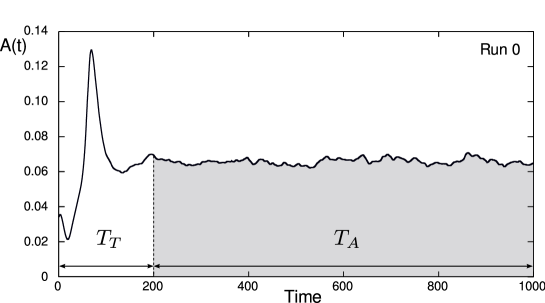
Figure 1: Integral velocity perturbations amplitude [32] for DNS of turbulent flow in a straight pipe, $\mbox{Re}_{D}=6000$; averaging over the single flow.

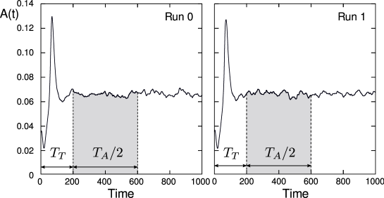
Figure 2: Integral velocity perturbations amplitude [32] for DNS of turbulent flow in a straight pipe, $\mbox{Re}_{D}=6000$; averaging over two flows.

2.2 Time integration schemes

The system of governing equations for direct numerical simulation of isothermal incompressible viscous flows consists of Navier-Stokes and continuity equations:

$$\frac{\partial{\bf{u}}}{\partial t}+{\bf{u}}\cdot\nabla{\bf{u}}=-\nabla p+\frac{1}{\mbox{Re}}\nabla^{2}{\bf{u}},$$ (1)

$$\nabla\cdot{\bf{u}}=0,$$ (2)

where $\bf{u}$ is the velocity field, $p$ is the pressure, and $t$ is the time. Equations (1)-(2) are written in the dimensionless form. The nondimensional Reynolds number is defined as $\mbox{Re}=UL/\nu$, where $U$ is the characteristic velocity, $L$ is the characteristic length scale, and $\nu$ is the kinematic viscosity of the fluid.

Let us consider the time integration schemes used for direct numerical simulations. The high order explicit or semi-implicit Runge-Kutta schemes (e.g., [1, 2, 3]) are typically used for high-fidelity turbulent flow simulations in order to reduce the numerical dissipation effects. These schemes consist of several substeps (the number of substeps depends on the approximation order of the numerical scheme). With a certain degree of simplification, each substep is comprised of predicting preliminary velocity field from (1), and projecting obtained velocity field on the divergence-free space by solving (2), transformed to the pressure Poisson equation:

$$\tilde{\bf u}={\bf u}^{*}-\tau\nabla\tilde{p},$$ (3)

$$\nabla^{2}\tilde{p}=\frac{1}{\tau}\,\nabla\cdot{\bf{u}}^{*}.$$ (4)

Here ${\bf u}^{*}$ is the preliminary velocity, $\tilde{\bf u}$ is the divergence-free velocity at the end of the substep, $\tilde{p}$ is the pressure at the end of the substep, and $\tau$ is a variable related to the integration step.

The most time-consuming part for obtaining solution of (1)-(2) at the next time step relates to the solution of pressure Poisson equation (4). One can see the spatial discretization and the corresponding SLAE matrix for the elliptic equation remain constant in the case of the grid remaining unchanged during the simulation. The matrix coefficients are also independent of the velocity distribution and the divergence of the preliminary velocity field arise on the right-hand side of the SLAE only. This means having $m$ different preliminary velocity fields in (3), $m$ pressure fields can be performed simultaneously by solving the SLAE with $m$ RHS vectors.

Generally speaking, the suggested modification of the computational procedure can also be extended on the case of moving grids, when the grid transformation is a function of the time only (e.g., the grids with moving regions), but not the instantaneous velocity fields (e.g., adaptively refined meshes). This, however, provides an additional limitation to the time integration: all the flows must be synchronized by the time step and in time. This limitation may reduce the expected gains for the proposed transformation of the computational algorithm and should be analyzed in each case.

2.3 Theoretical estimates

The proposed above modification of the numerical procedure for simultaneous modelling of multiple turbulent flow states allows to obtain higher performance for solving SLAEs of the pressure Poisson equation (which are typically dominating in the overall computing time), but needs some additional computations. Let us consider the basic theoretical estimates for the proposed modification to analyze possible gains. The value of interest is the parameter $P_{m}$, the overall simulation speedup for the simultaneous modelling of $m$ turbulent flow states compared to the simulation of the single turbulent flow state. By this definition, the parameter is a ratio of the time to compute the whole simulation with single flow state, $\mathcal{T}_{1}$, to the one with $m$ flow states, $\mathcal{T}_{m}$,

$$P_{m}=\frac{\mathcal{T}_{1}}{\mathcal{T}_{m}}.$$ (5)

The Runge-Kutta time integration schemes have a fixed number of substeps thus providing close to constant computational complexity per time step during the simulation. Then, the simulation time can be estimated as:

$$\mathcal{T}_{m}=N_{m}t_{m},$$ (6)

where $N_{m}$ is the number of time steps to be modelled, and $t_{m}$ is the computation time per integration step with $m$ flow states. The time integration in DNS/LES is typically performed with constant or predominantly constant time step, $\tau$. As a result, the number of time steps can be expressed through the physical simulation time, $T_{m}$:

$$N_{m}=\frac{T_{m}}{\tau},$$ (7)

where $T_{m}=T_{T}+T_{A}/m$. Introducing the parameter $\beta=T_{A}/T_{T}$, the ratio of time averaging to transition interval, the expression (5) can be represented as:

$$P_{m}=\frac{1+\beta}{m+\beta}\frac{mt_{1}}{t_{m}}.$$ (8)

The first multiplier in (8) reflects the overhead to perform additional $(m-1)$ flow states transitions and the second multiplier accounts the simulation speedup for simultaneous modelling of $m$ flow states compared to $m$ successive computations.

The computation time per integration step is approximated as a sum of two factors: the time to solve SLAEs for the pressure Poisson equation, $t^{S}$, and the time to construct the temporal and spatial discretization of the governing equations, $t^{D}$:

$$t_{m}=t_{m}^{S}+t_{m}^{D}.$$ (9)

The time to construct the discretizations is expressed in proportion to the number of flow states,

$$t_{m}^{D}=mt_{1}^{D},$$ (10)

as no gain is expected here due to the simulations with multiple flow states. Introducing the parameter $\theta$, the fraction of the SLAE solver time in the integration step execution time, $\theta=t_{1}^{S}/t_{1}$, one can obtain the following expression:

$$\frac{mt_{1}}{t_{m}}=\frac{1}{\theta\left(\frac{mt_{1}^{S}}{t_{m}^{S}}\right)^{-1}+\left(1-\theta\right)}.$$ (11)

To complete, the expression for the SLAE solver time as a function of the number of RHS vectors must be provided. The iterative methods for solving elliptic SLAEs with matrix of the general form, specifically Krylov subspace and multigrid methods, are based on SpMV operations and operations with dense vectors, and the former ones typically dominate in the solution time. With some assumptions, the time to solve the SLAE with multiple RHS vectors can be approximated in proportion to the time for GSpMV operation with $m$ vectors. The GSpMV is a memory-bound operation and its execution time coincides with the volume of data transfers with the memory. The total volume of data transfers depends on the matrix storage format, and the choice of the optimal one is affected by lots of factors, i.e. the matrix size, the number of nonzero elements, subblock structure of nonzero elements, matrix topology, etc.

For the CRS data format [33], which, despite of its simplicity, is still among the most popular ones in real applications, the volume of data transfers can be calculated explicitly. Let us consider the square matrix A with $n$ rows and $nnz$ nonzero elements, and two dense matrices X and Y with $n$ rows and $m$ columns. The matrix A is stored in CRS format and the dense matrices X and Y are stored row-wise in single vectors. For the sake of simplicity the integer numbers are assumed 4 bytes and floating point numbers are 8 bytes. The C-like code for the GSpMV operation $\bf{Y}=\bf{A}\bf{X}$ with $m$ RHS vectors is presented in Figure 3.

⬇

GSpMV (Matrix *M, double *X, double *Y, int m)

{

int i, j1, j2, k, l;

double sum[m];

j1 = M->row[0]; // (1)

for(i = 0; i < M->n; i++)

{

j2 = M->row[i+1]; // (1)

for(l = 0; l < m; l++)

sum[l] = 0.;

for(j = j1; j < j2; j++)

{

k = M->col[j]; // (2)

for(l = 0; l < m; l++)

sum[l] += M->val[j] * X[k*m+l]; // (3) & (4)

}

j1 = j2;

for(l = 0; l < m; l++)

Y[i*m+l] = sum[l]; // (5)

}

}

Figure 3: C-like code for GSpMV operation with matrix stored in CRS format.

The memory traffic produced by the GSpMV operation consists of read / write operations with 5 arrays: (1) $(n+1)$ integers reads from the array row; (2) $nnz$ integers reads from the array col; (3) $nnz$ floating point numbers reads from the array val; (4) $m\cdot nnz$ floating point numbers reads from the array X; (5) $m\cdot n$ floating point numbers writes to the array Y. In total, the GSpMV operation with $m$ vectors produces the data transfer with the memory equal to (single memory read in (1) is omitted):

$${\sum}_{m}=4n(2m+1)+12nnz+8m\cdot nnz.$$ (12)

The corresponding memory transfer gain is:

$$\frac{m{\sum}_{1}}{{\sum}_{m}}=\frac{m\left(5C+3\right)}{2m\left(C+1\right)+3C+1},$$ (13)

where $C=nnz/n$ is the average number of nonzero elements per matrix row. Taking into account, that typically $C\gg 1$, (13) can be reduced to a trivial expression:

$$\frac{m{\sum}_{1}}{{\sum}_{m}}\approx\frac{5m}{2m+3}.$$ (14)

Using (14) as an estimate for the SLAE solver execution times ratio in (11), the final expression can be achieved:

$$P_{m}=\frac{1+\beta}{m+\beta}\frac{5m}{5m-3\theta\left(m-1\right)}.$$ (15)

The presented estimate (15) is a function of three parameters: the times ratio $\beta$, the fraction of the SLAE solver time in the computation time per integration step $\theta$, and the number of averaging ensembles $m$. The parameter $\beta$ is a characteristic of the specific application modelled and is an input parameter for this estimate. The parameter $\theta$ is a characteristic of the numerical schemes and methods used for spatial and temporal discretization and solving SLAEs, and is also an input parameter. The parameter $m$ is a free parameter and it is reasonable to be chosen in order to maximize the simulation speedup. Differentiating expression (15) over $m$ one can obtain:

$$m^{*}=\sqrt{\frac{3\beta\theta}{5-3\theta}},$$ (16)

and the nearest integer value to $m^{*}$ can be treated as an expected optimal number of flow states, maximizing the overall simulation speedup.

The two limiting cases for (15) can be considered. In case the time averaging dominates over the transition, $\beta\gg 1$, (15) reduces to

$$P_{m}=\frac{5m}{5m-3\theta\left(m-1\right)},$$ (17)

that suggests more than 2-fold speedup can be achieved by the simultaneous modelling of several flow states. In the opposite case when the transition dominates over the time averaging, $\beta\ll 1$, (15) transforms to

$$P_{m}=\frac{5}{5m-3\theta\left(m-1\right)}.$$ (18)

Expression (18) means that the overall simulation slowdown is expected and the proposed idea is inapplicable for this type of problems.

Several reference values for the estimated simulation speedup with modelling multiple flow states are presented in Figure 4. The parameter $\theta$ here is set to $\theta=0.85$, which is an average of the values obtained in the numerical experiments considered in the validation section, where the SLAE solver input to the overall simulation time varied from 75 to 95%. The second parameter $\beta$ varies from 1 to 40. The presented figure demonstrates that the optimal number of flow states depends on the times ratio $\beta$ and changes from $m=2$ for $\beta=2-5$ to $m=4$ for $\beta=10-20$ and to $m=8$ for $\beta=40$. The expected speedup for $\beta=5-40$ is about 15-54%.

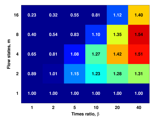
Figure 4: The estimated simulation speedup, $P_{m}$, as a function of the times ratio, $\beta$, and the number of modelled flow states, $m$.

It should be noted that the proposed estimate for the SLAE solver speedup due to its simplicity ignores several important aspects, like vectorization, regularization of memory access pattern and improvements of cache miss rate. Solution of SLAE with multiple RHS vectors also has a significant advantage for parallel computations, allowing to increase the amount of computations used to hide the MPI communications latency for non-blocking point-to-point communications. The number of RHS vectors affects the message sizes, but not the total amount of the messages, thus only slightly increasing the message transfer time.

The physical constraint of choosing the number of flow states should be considered in addition to the estimate (15). The time averaging interval per each flow state, $T_{A}/m$, must be preserved larger than the characteristic time scale of the modelled turbulent flow. This treatment provides the upper bound for the parameter $m$. In general, the typical time averaging interval $T_{A}$ is chosen to cover several tens to hundreds of characteristic time scales in order to obtain reliable statistics. The expected optimal number of flow states maximizing the simulation speedup is typically of order $\mathcal{O}(1)$ (see Figure 4). This means the time averaging interval $T_{A}/m$ would generally cover at least several characteristic time scales.

The use of computations with multiple RHS vectors increases the memory consumption per each compute node. The memory consumption scales proportionally to the number of flow states, except the information related to the simulated problem statement, which can be stored only once. This aspect may limit the applicability of the suggested approach in the case of huge computational grids and low memory capacity of the compute nodes scheduled for the simulation. However, the use of large grid blocks per node would require extremely long execution times for the whole simulation. The codes for DNS/LES usually demonstrate good scalability across multiple nodes with the granularity of lower than 100 thousand cells per node (e.g. [34, 35]). This allows to store in the memory without in due difficulties the data for several tens of flow states.

Accordingly, the proposed simple estimates demonstrate the possibility of the DNS/LES computations speedup by the simultaneous modelling of several independent flow states with subsequent post-processing of simulation results. While the speedup of only 15-54% is predicted by the estimates, even these results can be of high practical importance as typical high-fidelity turbulent flow simulations for the objects with complex geometry may take months to complete.

3 Numerical methods and software

To validate the proposed computational procedure and demonstrate the simulation speedup with modelling of multiple flow states the corresponding application for direct numerical simulation of turbulent flows and the SLAE solver were developed. The DNS application is an extension of “in-house” code for modelling incompressible turbulent flows. The code is based on the finite difference scheme for structured grids, and operates with arbitrary curvilinear orthogonal coordinates [36]. The second order central difference scheme on the staggered grid, preserving the discrete kinetic energy conservation property, is used for the spatial discretization. The time integration is performed by 3-1/3 step semi-implicit Runge-Kutta scheme with optimal time stepping algorithm [2]. The message passing programming model (MPI) is used to parallelize the computations. The simple 3D geometrical decomposition into equally sized subdomains is applied to distribute the problem across the computational processes.

The SparseLinSol library [37], containing a set of Krylov subspace and multigrid iterative methods, is used to solve the systems of linear algebraic equations. The corresponding extension for solving systems with multiple RHS vectors was developed. The library is based on hybrid multilevel parallel algorithms, accounting memory hierarchy optimal access pattern with four logical levels: “compute node / socket / numa-node / core” for CPUs with intra-node communications and synchronizations via POSIX Shared Memory. The library functionality allows efficient coupling with applications designed under several parallel programming models, including the pure MPI approach.

4 Validation results

Table 1: Parameters of the computational grids.

	Grid 1	Grid 2	Grid 3
Overall	$144\times 112\times 144$	$240\times 168\times 240$	$360\times 252\times 360$
Cube	$52\times 48\times 52$	$100\times 74\times 100$	$150\times 120\times 150$
$\Delta x$, $\Delta z$	$0.0065h-0.054h$	$0.0031h-0.038h$	$0.0024h-0.023h$
$\Delta y$	$0.0054h-0.07h$	$0.003h-0.044h$	$0.0023h-0.03h$
$\Delta y^{+}_{top}$	$1.50$	$1.10$	$0.98$

The efficiency of the formulated computational procedure and correctness of the proposed theoretical estimates are validated with two test cases including the modelling of incompressible turbulent flow in a plain channel [2] and in a channel with a matrix of wall-mounted cubes [38, 39, 40, 41]. For the first case, the flow is modelled in a rectangular computational domain of size $2\pi h\times 2h\times\pi h$ (Figure 5), where $h$ is the channel half-height, with periodic boundary conditions on streamwise and spanwise directions and no-slip conditions on the channel walls. The constant flow rate is preserved during the simulation with the Reynolds number $\mbox{Re}_{b}=2800$, where $\mbox{Re}_{b}=U_{b}h/\nu$ is defined using the bulk velocity $U_{b}$ and the channel half-height $h$. The simulation is performed on the computational grid of $160\times 140\times 160$ cells (3.58 mln. cells). The grid is uniform in streamwise and spanwise directions, and the grid stretching is applied in the wall-normal direction with the ratio $\Delta y_{max}/\Delta y_{min}=5$. Introducing the viscous length scale $l_{\tau}=\nu/u_{\tau}$, where $u_{\tau}=\sqrt{\tau_{w}/\rho}$ is the friction velocity, and $\tau_{w}$ is the mean wall shear stress, one can express the grid spacings in wall units. The corresponding values are: $\Delta x^{+}=6.95$, $\Delta y^{+}=0.81-4.1$, $\Delta z^{+}=3.48$. The chosen grid resolution corresponds to the typical grid spacings, used for DNS of turbulent channel flows, e.g. [2, 30].

The second case considers the turbulent flow over the dedicated cube in the channel (Figure 6), with periodic boundary conditions along the two spatial directions and no-slip boundary conditions on the rigid walls. The computational domain is set to $4h\times 3.4h\times 4h$, where $h$ is the cube height. The constant flow rate is considered with the Reynolds number $\mbox{Re}_{b}=3854$, defined using the bulk velocity $U_{b}$ and the cube height $h$. The computations are performed on three grids, consisting of approximately 2.32, 9.68, and 32.7 mln. cells. The parameters of the grids are specified in Table 1. The table also contains the $\Delta y^{+}$ values for the grid spacings at the top wall of the channel, where the viscous length scale is defined using the mean shear stress at this wall. For the other walls the only local viscous length scales can be used to provide reference information about the grid resolution. The mean grid spacings near the walls are $\Delta x_{i}^{+}\lesssim 2.4$, $1.34$, and $1.18$ for Grid 1, Grid 2, and Grid 3 correspondingly. The maximum values are three times higher than the mean ones, but they are observed in a few cells around the edges of the cube only. The grids of 2.32 and 9.68 mln. cells are used for the detailed step by step validation of the proposed computational methodology. For the finest grid the only single run is performed to demonstrate the grid independence for the obtained turbulent flow characteristics.

Figure 5: Sketch of the computational domain for the problem of modelling the turbulent flow in a plain channel.

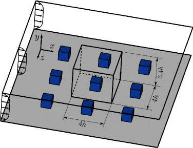
Figure 6: Sketch of the computational domain for the problem of modelling the turbulent flow in a channel with a matrix of wall-mounted cubes.

The presented validation results were obtained on two supercomputers “Lomonosov” and “Lomonosov-2”. The “Lomonosov” supercomputer contains the nodes with two 4-core Intel Xeon X5570 processors and 12 GB RAM, connected by QDR InfiniBand network. The “Lomonosov-2” supercomputer is equipped with the nodes containing single 14-core Intel Xeon E5-2697v3 processor, 64 GB RAM, and FDR InfiniBand interconnect. Accordingly, the SparseLinSol library was configured to perform the calculations with 3-level hybrid model (computational node / socket / core) for “Lomonosov” supercomputer and 2-level hybrid model (computational node / core) for “Lomonosov-2” supercomputer, which allowed to utilize efficiently all available cores per node. The results presented below were obtained running 8 and 14 computational processes per node correspondingly, i.e. using each CPU core.

The effectiveness of the parallel computations is analyzed in terms of parallel efficiency. This metric is defined as:

$$E(p)=\frac{T_{1}}{p\,T_{p}},$$ (19)

where $p$ is the number of computing units, $T_{1}$ is the execution time using single computing unit, and $T_{p}$ is the execution time using $p$ computing units. The computing unit relates to the minimal number of computational resources used to perform the simulation. For the second test case performed on the coarse grid the computing unit is equal to single node and for the other problems it is equal to 8 nodes.

4.1 Solution of SLAE with multiple RHS vectors

The efficiency of the developed SLAE solver with multiple RHS vectors is investigated for three matrices, which correspond to the discretized pressure Poisson equation for different test cases and computational grids. The BiCGStab iterative method with classical algebraic multigrid preconditioner is used to solve the test systems. The PT-Scotch graph partitioning library [42] is applied to build the sub-optimal matrix decomposition. In order to avoid the slight variance in the number of iterations for convergence, the fixed number of iterations is simulated for benchmarking purposes.

The computational times for one iteration of SLAE solver and the corresponding performance gains due to the use of operations with blocks of vectors are presented in Tables 2 and 3. As expected, the solution of SLAE with multiple RHS vectors allows to improve the efficiency of the calculations and reduce the computational time. The measured performance gains for both test cases are in a good agreement with the proposed theoretical estimate (14), based on the memory traffic reduction.

Table 2: Theoretical and measured performance gains for solving SLAE with multiple RHS vectors. Test matrix for the problem of modelling turbulent flow in a plain channel, “Lomonosov” supercomputer, 8 nodes.

RHS	Time, s	Gain	Estimate (14)
1	0.05	-	-
2	0.07	1.45	1.48
4	0.10	1.86	1.95
8	0.18	2.12	2.21
16	0.32	2.45	2.29

Table 3: Theoretical and measured performance gains for solving SLAE with multiple RHS vectors. Test matrices for the problem of modelling turbulent flow in a channel with a matrix of wall-mounted cubes, “Lomonosov-2” supercomputer.

RHS	Grid 1 (1 node)		Grid 2 (8 nodes)		Estimate (14)
	Time, s	Gain	Time, s	Gain
1	0.12	-	0.51	-	-
2	0.16	1.45	0.69	1.48	1.48
4	0.25	1.86	1.05	1.92	1.95
8	0.44	2.13	1.87	2.17	2.21
16	0.79	2.37	3.58	2.26	2.29

The parallel efficiency results for 1, 4, and 16 RHS vectors for the cases considered are presented in Figures 7 and 8. The plots demonstrate the improvement in parallel efficiency for the simulations with multiple RHS vectors. The scalability for single RHS vector degrade faster compared to other runs. For example, the parallel efficiency of only 66% for 64 nodes is obtained for the test problem of 2.32 mln. cells, while for 4 and 16 RHS vectors it reaches about 81% and 98% respectively. This tendency affects the performance gain for multi-node runs when solving SLAE with multiple RHS vectors: for 64 nodes it increases up to 2.29 and 3.52 correspondingly, indicating an additional advantage of using the operations with blocks of vectors for parallel runs. The same behaviour is observed for two other test problems of 3.58 and 9.68 mln. cells with only the difference that the degradation of parallel efficiency is shifted towards the higher scales.

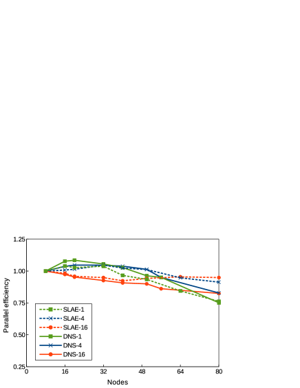
Figure 7: Parallel efficiency of the linear solver (SLAE) and the DNS application (DNS) performed with 1, 4, and 16 flow states. Test problem of modelling turbulent flow in a plain channel, “Lomonosov” supercomputer.

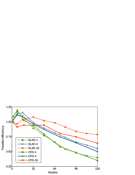
Figure 8: Parallel efficiency of the linear solver (SLAE) and the DNS application (DNS) performed with 1, 4, and 16 flow states. Test problem of modelling turbulent flow in a channel with a matrix of wall-mounted cubes, Grid 1 (left) and Grid 2 (right), “Lomonosov-2” supercomputer.

4.2 Simultaneous modelling of multiple flow states

Table 4: Theoretical and measured performance gains for modelling the single time step for multiple flow states. Test problem of modelling turbulent flow in a plain channel, “Lomonsov” supercomputer, 8 nodes.

RHS	Time, s	Gain	Estimate (11)
1	1.06	-	-
2	1.58	1.35	1.32
4	2.59	1.64	1.56
8	4.70	1.81	1.72
16	8.35	2.04	1.82

Table 5: Theoretical and measured performance gains for modelling the time step for multiple flow states. Test problem of modelling turbulent flow in a channel with a matrix of wall-mounted cubes, “Lomonosov-2” supercomputer.

States	Grid 1 (1 node)		Grid 2 (8 nodes)		Estimate (11)
	Time, s	Gain	Time, s	Gain
1	2.78	-	1.53	-	-
2	4.09	1.36	2.26	1.36	1.32
4	6.73	1.63	3.84	1.60	1.56
8	12.14	1.81	7.02	1.75	1.72
16	22.38	1.96	13.10	1.87	1.82

Table 6: Memory consumption for simultaneous modelling of multiple flow states, in MB per computational core. Test problem of modelling turbulent flow in a channel with a matrix of wall-mounted cubes, Grid 1, “Lomonosov-2” supercomputer.

States	1 node	4 nodes	16 nodes
1	330	145	162
2	460	180	172
4	720	250	190
8	1170	385	230
16	2120	655	312
Approximation	$200+130m$	$110+35m$	$150+10m$

Table 7: Memory consumption for simultaneous modelling of multiple flow states, in MB per computational core. Test problem of modelling turbulent flow in a channel with a matrix of wall-mounted cubes, Grid 2, “Lomonosov-2” supercomputer.

States	8 nodes	16 nodes	32 nodes
1	305	222	276
2	375	256	294
4	505	324	330
8	770	468	404
16	1230	758	560
Approximation	$240+65m$	$188+35m$	$258+18m$

A series of short runs performing several time steps for the DNS application is calculated to investigate the simulation speedup when modelling multiple flow states. As the input of the SLAE solver for pressure Poisson equation is dominating in the overall simulation time, the strong correlation between the parallel efficiency for the SLAE solver and the DNS application results is expected. These expectations are confirmed by the corresponding calculations.

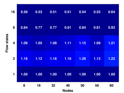
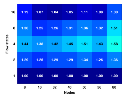
Figure 9: Overall performance gain estimate (8) based on the single time step simulation results. Test problem of modelling turbulent flow in a plain channel. Left – $\beta=5$; right – $\beta=20$.

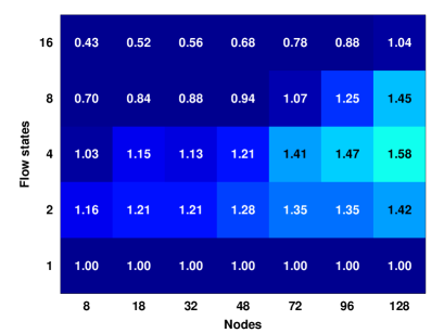
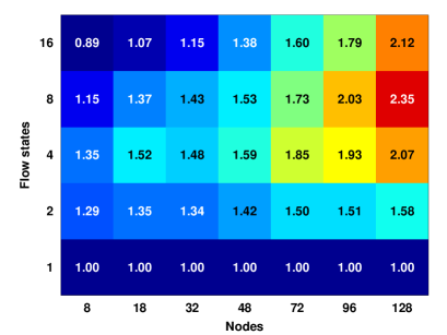
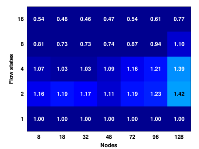
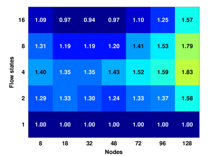
Figure 10: Overall performance gain estimate (8) based on the single time step simulation results. Test problem of modelling turbulent flow in a channel with a matrix of a wall-mounted cubes. Top row – results for Grid 1; bottom row – results for Grid 2. Left column – $\beta=5$; right column – $\beta=20$.

The execution times per integration step, as well as performance gain results, are summarized in Tables 4 and 5. The obtained performance gains are similar for all the cases and computational grids and correspond to the estimates (11). The parallel efficiency results for the DNS application runs are presented in Figures 7 and 8. They replicate the ones for the SLAE solver with only minor differences, mostly caused by different data decomposition strategies used in standalone SLAE solver and in DNS application.

The simulations with multiple flow states increase the memory consumption during the computations. The memory profiling is performed to estimate the upper bound for the maximum number of simultaneously modelled flow states in terms of memory consumption. The memory usage results for two computational grids and with varying number of compute nodes are presented in Tables 6 and 7. The obtained results can be approximated by the simple formula:

$$M=\alpha+\gamma\cdot m,$$ (20)

where $M$ is the memory consumption per core, $\alpha$ is the memory to store the service information shared among all flow states (model description, computational grid, SLAE solver data, etc.), and $\gamma$ is the memory to store the data for the single flow state. The suggested approximation shows that the second parameter, $\gamma$, is in proportion to the local grid block size and decreases linearly with the number of nodes. The compute nodes of “Lomonosov-2” supercomputer provide about 4.6 GB of RAM per core. For example, for the Grid 2 performed on 32 nodes (448 cores) the memory consumption per each flow state does not exceed 18 MB/core (or 252 MB/node). This means the simulations with several hundred flow states can be performed without in due difficulties on “Lomonosov-2” compute nodes. The obtained profiling results allow to state that the memory consumption does not provide any discernible limitations on the applicability of the proposed approach.

The measured DNS application performance gain results are used to adjust the overall simulation speedup estimates (8). The corresponding distributions for the cases considered are presented in Figures 9 and 10 for $\beta=5$ and $\beta=20$. These results outperform the theoretical estimates in Figure 4 and show the potential of 2x speedup for the overall simulation.

4.3 Full-scale DNS

The several full-scale turbulent flow simulations for two test cases are considered in this section to demonstrate the correctness of the proposed theoretical estimates and real simulation speedup, and validate the simulation results obtained as a result of averaging over different number of ensembles.

4.3.1 DNS of turbulent flow in a plain channel

The two simulations are performed for the problem of modelling turbulent flow in a plain channel. The overall simulation interval for these runs is set to $T=3000$ time units, which comprises transition interval of $T_{T}=500$ units and time averaging interval of $T_{A}=2500$ units with the corresponding times ratio parameter $\beta=5$. The initial velocity field is specified in the form of laminar Poiseuille flow with periodic perturbations for $x$- and $z$-velocity components along the spanwise and streamwise directions:

$$u_{i}=\left(1-\left(\frac{y-h}{h}\right)^{2}\right)\left(\frac{3}{2}+\delta_{i}\sin\left(\frac{2\pi z}{L_{z}}\right)\right),\ i=0,\ldots,m-1,$$ (21)

$$w_{i}=\delta_{i}\left(1-\left(\frac{y-h}{h}\right)^{2}\right)\sin\left(\frac{2\pi x}{L_{x}}\right),\ i=0,\ldots,m-1,$$ (22)

where $L_{x}=2\pi h$, $L_{z}=\pi h$, $\delta_{i}\in\left[-0.1,0.1\right]$ is a random number, and $i$ is the flow state index.

The full-scale runs are simulated using 40 compute nodes with single and two simultaneously modelled flow states. According to the estimates presented in Figure 9, performance gain by a factor of 1.16 is expected for this test case configuration. The real simulation times for these two runs are 480 min. and 412 min. correspondingly, that is the performance gain is equal to 1.17. The estimate based on the single time step simulation results correctly predicts the overall simulation speedup.

The obtained turbulent flow characteristics are compared with the data, presented in [43]. The friction Reynolds numbers, $\mbox{Re}_{\tau}=u_{\tau}h/\nu$, for the performed simulations are $\mbox{Re}_{\tau}^{1}=176.93$ and $\mbox{Re}_{\tau}^{2}=177.01$, which are within 1% error with respect to the reference value $\mbox{Re}_{\tau}=178.13$. The comparison of the second order statistics includes distributions of rms velocity profiles for three components obtained in two simulations together with the data of Moser et al. [43]. The results shown in Figure 11 are in good agreement with each other and with reference data.

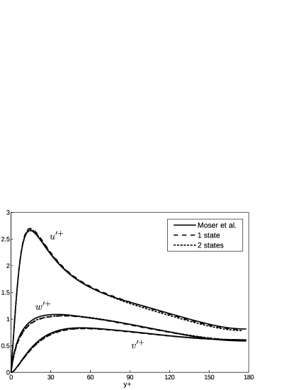
Figure 11: Rms velocity distributions for the simulations with averaging over single and two flow states, and the reference data of Moser et al. [43]. Test problem of modelling turbulent flow in a plain channel.

4.3.2 DNS of turbulent flow over a matrix of wall-mounted cubes

The six full-scale runs are performed when modelling the turbulent flow over a matrix of wall-mounted cubes. In total, the interval of $T=2100$ time units is performed, which includes $T_{T}=100$ units of the initial transition and $T_{A}=2000$ units of averaging to collect the turbulent statistics. This problem setup corresponds to the times ratio parameter $\beta=20$. The preliminary streamwise velocity component in the interior of the computational domain is specified in the form:

$$u_{i}=1+\delta_{i}\left(1-2\{i/2\}\right)\sin\left(\frac{2\pi z}{L_{z}}\left(1+[i/2]\right)\right),\ i=0,\ldots,m-1,$$ (23)

where $L_{z}=4h$, $\delta_{i}\in\left[-0.05,0.05\right]$ is a random number, $i$ is the flow state index, and $\left[\alpha\right]$ and $\{\alpha\}$ are the integer and fractional parts of $\alpha$ respectively. To obtain initial flow states the preliminary velocity distributions are projected on the divergence-free space and adjusted to preserve the predefined flow rate.

The two runs with single and four simultaneously modelled flow states for Grid 1 are calculated on 32 nodes, with corresponding simulation times of 936 min. and 640 min. The obtained simulation speedup by a factor 1.46 coincides with the adjusted estimate in Figure 10, where the performance gain of 1.48 is predicted. The third run for Grid 1 with modelling of eight flow states is performed on 96 nodes. According to the estimates in Figure 10 and the parallel efficiency results in Figure 8, the simulation speedup by a factor of 3 is expected compared to the one with single flow state performed on 32 nodes. The execution time for this run is equal to 320 min., i.e. the speedup by a factor of 2.95 is obtained. These calculations also demonstrate good correspondence between the estimates and full-scale simulations.

The cross-correlation analysis is performed for the third run to demonstrate the correctness of the chosen transition interval and the fact that the initial turbulent flow states are uncorrelated. The time series for the velocity components monitored in several control points around and in the wake of the cube are analyzed. The cross-correlation function is defined as [44]:

$$\rho_{XY}=\frac{cov\left(X,Y\right)}{\sqrt{var\left(X\right)var\left(Y\right)}},$$ (24)

where $X$ and $Y$ are the segments of the velocities time series corresponding to different flow states, $cov(X,Y)$ is the covariance of $X$ and $Y$, and $var(X)$ is the variance of $X$. The time series $X$ and $Y$ are defined by two parameters, $t$ and $T_{0}$. The first one corresponds to the start time and the second one corresponds to the length of the time series. Figure 12 shows the cross-correlation distributions for the streamwise velocities obtained in four points for two flow states ($i=0$ and $i=1$) and with $T_{0}=50$. The presented results vividly demonstrate that these two flow states become uncorrelated at $t\sim 10$ which is lower than the transition interval $T_{T}=100$ chosen in the simulations. The cross-correlation coefficients for eight flow states for $t=100$ and $T_{0}=50$ are presented in Figure 13. This distribution also demonstrates that all eight initial turbulent flow states used for time averaging are uncorrelated.

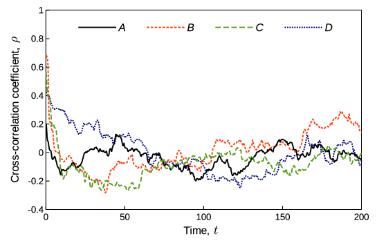
Figure 12: Cross-correlation distributions for streamwise velocity evolution in 4 control points: $A=\{0.73h,\ h,\ 0\}$, $B=\{0.73h,\ 0.8h,\ 0\}$, $C=\{1.07h,\ 0.52h,\ 0\}$, $D=\{1.54h,\ 0.52h,\ 0.51h\}$; the origin of the coordinate system is located at the bottom wall of the channel in the middle of the cube. The time series length is equal to $T_{0}=50$.

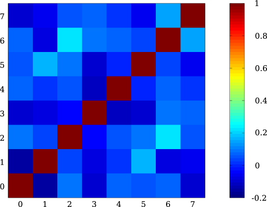
Figure 13: Cross-correlation matrix for streamwise velocity for eight initial turbulent flow states ($t=T_{T}=100$) for the data monitored in the control point $A=\{0.73h,\ h,\ 0\}$. Time series length is equal to $T_{0}=50$.

The two additional simulations are performed for the Grid 2 with 72 nodes for single and four flow states. The measured execution times are 4011 min. and 2625 min. with corresponding speedup by a factor of 1.53. This value is also in good agreement with the estimate, which predicted the performance gain equal to 1.52.

The turbulent flow characteristics, obtained in the simulations with simultaneous modelling of multiple flow states, are compared with traditional DNS results and with experimental data. The first and second order statistics in the $xy$-plane bisecting the cube are inspected. The corresponding mean streamwise velocity and Reynolds normal stress distributions along the channel for the Grid 1 with single flow state, Grid 2 with four flow states and the ones obtained in the experiments [38, 39] are presented in Figure 14. The difference between the simulation results for single and four flow states with different grids is almost indistinguishable for both mean velocity and Reynolds normal stress distributions. The observed variances between the numerical and experimental data coincide with the ones for the numerical simulation results of other authors [40, 41].

The streamwise Reynolds normal stress distributions for all the performed simulations are compared in Figure 15. The corresponding distributions located at the distance $0.3h$ from the trailing edge of the cube are examined. This figure also contains the DNS results [40] and experimental data [38]. The obtained simulation results are in good correspondence with the DNS results of other authors. The slight variance in the peak values of the Reynolds normal stress distributions for the numerical and experimental data is observed. This fact could be a result of some experimental measurements errors or minor differences in the experimental and numerical problem statements.

The simulations performed with varying number of flow states demonstrate some deviations in the second order characteristics. The corresponding distributions obtained as a result of averaging in time for each of four flow realizations performed in a single run are presented in Figure 16. The figure demonstrates observable variance for these distributions and suggests that better match between the single flow state and multiple flow state simulations can be expected for a longer time averaging interval.

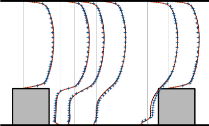
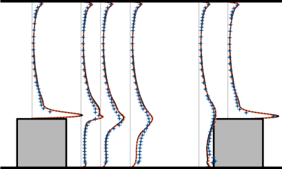
Figure 14: The mean streamwise velocity (left) and $\overline{u^{\prime 2}}$ Reynolds normal stress (right) distributions at the channel cross section bisecting the cube. Continuous line – Grid 1, averaging over single flow state; dashed line – Grid 2, averaging over four flow states; markers – experimental data.

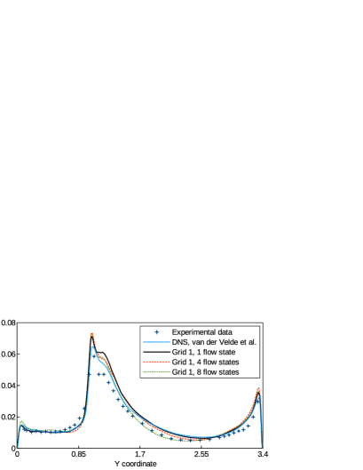
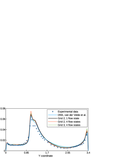
Figure 15: The $\overline{u^{\prime 2}}$ Reynolds normal stress distributions at the distance $0.3h$ from the trailing edge of the cube. Comparison of numerical simulation results for various computational grids and number of flow states, experimental data of Meinders [38], and DNS results of van der Velde et al. [40].

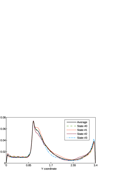
Figure 16: The $\overline{u^{\prime 2}}$ Reynolds normal stress distributions at the distance $0.3h$ from the trailing edge of the cube. Comparison of simulation results for four turbulent flow realizations performed in a single run, Grid 1.

The presented results indicate that the proposed numerical procedure with simultaneous modelling of multiple flow states allows to obtain a 1.5- to 2-fold speedup for DNS applications compared to the conventional approach with averaging over a single flow state due to better utilization of HPC hardware resources.

5 Discussion

The results presented in this paper can be considered as a proof of concept for the simultaneous modelling of multiple turbulent flow states approach to speedup the DNS/LES computations. Meanwhile, this paper not focuses on several important aspects which may lead to further simulation speedup improvements. These are briefly discussed in the current section.

The presented results clearly demonstrate that the overall simulation speedup is strongly dependent on the times ratio parameter, $\beta$. An approach applied in this paper to obtain multiple independent initial turbulent flow states produces significant overhead, thus reducing the benefits of the proposed computational methodology. Various techniques can be applied to reduce computational costs to obtain these initial flow states. Among them can be an approach based on introduction of perturbations to the statistically steady turbulent flow obtained for the single flow state. The simulations on a series of nested computational grids with rescaling of results can also help to provide multiple initial turbulent flow states with lower computational costs.

The validation results presented in this paper are obtained on the supercomputers with Intel processors. The corresponding GSpMV operation speedup coincides with the memory traffic reduction estimates and the expected maximum is about 2.5. The results obtained in [25] show the same values for the Intel-based compute system. However, for the system with Sparc processors the observed performance gain is three times higher, about 7.6. This indicates the efficiency of the proposed method on some HPC systems can significantly outperform presented in the paper performance gain results.

An interesting observation is discussed in [27]. The authors noted that the averaging over multiple realizations of the same turbulent flow (ensemble averaging) may provide higher accuracy compared to the conventional long-range simulation and averaging in time. This results in a suggestion that the same accuracy of statistics for multiple flow states simulations can be obtained by performing shorter overall time averaging interval. This observation is not accounted in this paper, but can be an additional source of improvement for the proposed computational procedure.

The current paper discusses the applicability of the proposed approach to standard DNS or LES methods. These methods, however, do not exhaust the range of possible applications to high-fidelity turbulent flow modelling methods. For example, the quasi-DNS approach (QDNS) [45] can be marked as a good candidate to use the same methodology. The QDNS approach combines the main LES modelling with multiple subscale near-wall DNS runs, performed to account the influence of the walls. The corresponding DNS runs are independent and can be computed in a single run with multiple flow states. Moreover, this algorithm has no drawbacks related to simulation of transition interval to generate initial turbulent flow states for these DNS runs.

6 Conclusions

The modified computational procedure for numerical simulation of turbulent flows is presented. The suggested algorithm is based on the idea of simultaneous modelling of multiple turbulent flow states followed by averaging of the simulation results. The proposed approach allows to parallelize the transient simulation in time and to use for the pressure Poisson equation the SLAE solver operating with multiple right-hand side vectors. The simple theoretical performance gain estimate, based on the memory traffic reduction for matrix-vector operations with blocks of vectors, is formulated. The estimate uses only two application-specific input parameters and allows to outline the range of applicability for the proposed computational procedure and to predict the simulation speedup. The speedup by a factor of 1.5 is expected with some typical range of input parameters.

The extension of the SparseLinSol library, allowing to solve the systems of linear algebraic equations with blocks of RHS vectors, and the application for direct numerical simulation of turbulent flows are developed. The developed software is applied to model the turbulent flow in the plain channel and in the channel with a matrix of wall-mounted cubes, which are used to validate in detail the formulated estimate and the proposed algorithm.

The step by step validation results of solving SLAE with multiple RHS vectors and modelling the single DNS application time step show good correspondence between the theoretical and numerical results. For several nodes runs the speedup by a factor of 1.5 is observed. The larger scale runs including several tens of compute nodes outperform the estimate thanks to the better scalability of the SLAE solver operating with multiple RHS vectors.

Several full-scale DNS runs for two test cases, various computational grids, variable number of compute nodes and computing systems, and number of modelled flow states are performed. The observed performance gain results correspond to the estimates, and the overall simulation speedup by a factor of 2 is demonstrated. The presented turbulent flow characteristics for the full-scale runs coincide with each other and are in agreement with the experimental data and results presented by other authors. These facts vividly demonstrate the correctness and the efficiency of the proposed numerical procedure for modelling incompressible turbulent flows and the potential of 2x speedup for large-scale turbulent flow simulations.

References

- [1] P. R. Spalart, R. D. Moser, M. M. Rogers, Spectral methods for the Navier-Stokes equations with one infinite and two periodic directions, Journal of Computational Physics 96 (2) (1991) 297–324. doi:https://doi.org/10.1016/0021-9991(91)90238-G.
- [2] N. Nikitin, Third-order-accurate semi-implicit Runge-Kutta scheme for incompressible Navier-Stokes equations, International Journal for Numerical Methods in Fluids 51 (2) (2006) 221–233. doi:10.1002/fld.1122.
- [3] F. X. Trias, O. Lehmkuhl, A self-adaptive strategy for the time integration of Navier-Stokes equations, Numerical Heat Transfer, Part B: Fundamentals 60 (2) (2011) 116–134. doi:10.1080/10407790.2011.594398.
- [4] P. Moin, W. C. Reynolds, J. H. Ferziger, Large eddy simulation of incompressible turbulent channel flow, Tech. Rep. TF-12., Dept Mech. Engng, Stanford Univ. (1978).
- [5] P. Moin, J. Kim, Numerical investigation of turbulent channel flow, Journal of Fluid Mechanics 118 (1982) 341–377. doi:10.1017/S0022112082001116.
- [6] K. Mahesh, G. Constantinescu, P. Moin, A numerical method for large-eddy simulation in complex geometries, Journal of Computational Physics 197 (1) (2004) 215–240. doi:10.1016/j.jcp.2003.11.031.
- [7] D. Kim, H. Choi, A second-order time-accurate finite volume method for unsteady incompressible flow on hybrid unstructured grids, Journal of Computational Physics 162 (2) (2000) 411 – 428. doi:https://doi.org/10.1006/jcph.2000.6546.
-
[8]
P. Swarztrauber, A direct method for
the discrete solution of separable elliptic equations, SIAM Journal on
Numerical Analysis 11 (6) (1974) 1136–1150.
URL http://www.jstor.org/stable/2156231 - [9] A. Gorobets, F. Trias, M. Soria, A. Oliva, A scalable parallel Poisson solver for three-dimensional problems with one periodic direction, Computers and Fluids 39 (3) (2010) 525–538. doi:10.1016/j.compfluid.2009.10.005.
- [10] U. Trottenberg, C. Oosterlee, A. Schuller, Multigrid, Academic Press, New York, 2001.
- [11] H. A. van der Vorst, Bi-CGSTAB: A fast and smoothly converging variant of Bi-CG for the solution of nonsymmetric linear systems, SIAM Journal on Scientific and Statistical Computing 13 (2) (1992) 631–644. doi:10.1137/0913035.
- [12] L. T. Yang, R. P. Brent, The improved BiCGStab method for large and sparse unsymmetric linear systems on parallel distributed memory architectures, in: Fifth International Conference on Algorithms and Architectures for Parallel Processing, 2002. Proceedings, 2002, pp. 324–328. doi:10.1109/ICAPP.2002.1173595.
- [13] B. Krasnopolsky, The reordered BiCGStab method for distributed memory computer systems, Procedia Computer Science 1 (1) (2010) 213–218. doi:10.1016/j.procs.2010.04.024.
- [14] Y. Saad, M. H. Schultz, GMRES: A generalized minimal residual algorithm for solving nonsymmetric linear systems, SIAM Journal on Scientific and Statistical Computing 7 (3) (1986) 856–869. doi:10.1137/0907058.
- [15] A. H. Baker, R. D. Falgout, T. Gamblin, T. V. Kolev, M. Schulz, U. M. Yang, Scaling algebraic multigrid solvers: On the road to exascale, in: C. Bischof, H.-G. Hegering, W. Nagel, G. Wittum (Eds.), Competence in High Performance Computing 2010, Springer-Verlag, 2012, pp. 215–226. doi:10.1007/978-3-642-24025-6_18.
- [16] W. D. Gropp, D. K. Kaushik, D. E. Keyes, B. F. Smith, Toward realistic performance bounds for implicit CFD codes, in: Proceedings of Parallel CFD’99, Elsevier, 1999, pp. 233–240.
- [17] S. Williams, L. Oliker, R. Vuduc, J. Shalf, K. Yelick, J. Demmel, Optimization of sparse matrix-vector multiplication on emerging multicore platforms, in: Proceedings of the 2007 ACM/IEEE Conference on Supercomputing, SC’07, ACM, New York, NY, USA, 2007, pp. 38:1–38:12. doi:10.1145/1362622.1362674.
- [18] S. Williams, A. Waterman, D. Patterson, Roofline: An insightful visual performance model for multicore architectures, Commun. ACM 52 (4) (2009) 65–76. doi:10.1145/1498765.1498785.
- [19] A. Buluç, J. T. Fineman, M. Frigo, J. R. Gilbert, C. E. Leiserson, Parallel sparse matrix-vector and matrix-transpose-vector multiplication using compressed sparse blocks, in: Proceedings of the Twenty-first Annual Symposium on Parallelism in Algorithms and Architectures, SPAA’09, ACM, New York, NY, USA, 2009, pp. 233–244. doi:10.1145/1583991.1584053.
- [20] A. N. Yzelman, R. H. Bisseling, Cache-oblivious sparse matrix-vector multiplication by using sparse matrix partitioning methods, SIAM Journal on Scientific Computing 31 (4) (2009) 3128–3154. doi:10.1137/080733243.
- [21] M. Martone, Efficient multithreaded untransposed, transposed or symmetric sparse matrix-vector multiplication with the Recursive Sparse Blocks format, Parallel Computing 40 (7) (2014) 251–270, 7th Workshop on Parallel Matrix Algorithms and Applications. doi:10.1016/j.parco.2014.03.008.
- [22] M. Kreutzer, G. Hager, G. Wellein, H. Fehske, A. R. Bishop, A unified sparse matrix data format for efficient general sparse matrix-vector multiplication on modern processors with wide SIMD units, SIAM Journal on Scientific Computing 36 (5) (2014) C401–C423. doi:10.1137/130930352.
- [23] X. Liu, E. Chow, K. Vaidyanathan, M. Smelyanskiy, Improving the performance of dynamical simulations via multiple right-hand sides, in: 2012 IEEE 26th International Parallel and Distributed Processing Symposium, 2012, pp. 36–47. doi:10.1109/IPDPS.2012.14.
- [24] H. M. Aktulga, A. Buluç, S. Williams, C. Yang, Optimizing sparse matrix-multiple vectors multiplication for nuclear configuration interaction calculations, in: 2014 IEEE 28th International Parallel and Distributed Processing Symposium, 2014, pp. 1213–1222. doi:10.1109/IPDPS.2014.125.
- [25] S. Imamura, K. Ono, M. Yokokawa, Iterative-method performance evaluation for multiple vectors associated with a large-scale sparse matrix, International Journal of Computational Fluid Dynamics 30 (6) (2016) 395–401. doi:10.1080/10618562.2016.1234046.
- [26] Y. Feng, D. Owen, D. Perić, A block conjugate gradient method applied to linear systems with multiple right-hand sides, Computer Methods in Applied Mechanics and Engineering 127 (1) (1995) 203 – 215. doi:10.1016/0045-7825(95)00832-2.
- [27] V. Makarashvili, E. Merzari, A. Obabko, A. Siegel, P. Fischer, A performance analysis of ensemble averaging for high fidelity turbulence simulations at the strong scaling limit, Computer Physics Communications 219 (2017) 236–245. doi:10.1016/j.cpc.2017.05.023.
- [28] B. Galanti, A. Tsinober, Is turbulence ergodic?, Physics Letters A 330 (3-4) (2004) 173–180. doi:10.1016/j.physleta.2004.07.009.
- [29] A. Tsinober (Ed.), An Informal Conceptual Introduction to Turbulence, 2nd Edition, Vol. 92 of Fluid Mechanics and Its Applications, Springer Netherlands, 2009. doi:10.1007/978-90-481-3174-7.
- [30] N. Nikitin, Disturbance growth rate in turbulent wall flows, Fluid Dynamics 44 (5) (2009) 27–32. doi:10.1134/S0015462809050032.
- [31] G. Nastac, J. W. Labahn, L. Magri, M. Ihme, Lyapunov exponent as a metric for assessing the dynamic content and predictability of large-eddy simulations, Physical Review Fluids 2 (9) (2017) 094606. doi:10.1103/PhysRevFluids.2.094606.
- [32] T. V. Voronova, N. V. Nikitin, Direct numerical simulation of the turbulent flow in an elliptical pipe, Computational Mathematics and Mathematical Physics 46 (8) (2006) 1378–1386. doi:10.1134/S0965542506080094.
- [33] Y. Saad, Iterative Methods for Sparse Linear Systems, 2nd Edition, Society for Industrial and Applied Mathematics, 2003. doi:10.1137/1.9780898718003.
- [34] R. Borrell, J. Chiva, O. Lehmkuhl, G. Oyarzun, I. Rodríguez, A. Oliva, Optimising the termofluids cfd code for petascale simulations, International Journal of Computational Fluid Dynamics 30 (6) (2016) 425–430. doi:10.1080/10618562.2016.1221503.
- [35] N. Offermans, O. Marin, M. Schanen, J. Gong, P. Fischer, P. Schlatter, A. Obabko, A. Peplinksi, M. Hutchinson, E. Merzari, On the Strong Scaling of the Spectral Element Solver Nek5000 on Petascale Systems, ArXiv e-printsarXiv:1706.02970, doi:10.1145/2938615.2938617.
- [36] N. Nikitin, Finite-difference method for incompressible Navier-Stokes equations in arbitrary orthogonal curvilinear coordinates, J. Comput. Phys. 217 (2) (2006) 759–781. doi:10.1016/j.jcp.2006.01.036.
- [37] B. Krasnopolsky, A. Medvedev, Acceleration of large scale OpenFOAM simulations on distributed systems with multicore CPUs and GPUs, in: Parallel Computing: On the Road to Exascale, Vol. 27 of Advances in Parallel Computing, NIEUWE HEMWEG 6B, AMSTERDAM, NETHERLANDS, 1013 BG, 2016, pp. 93–102. doi:10.3233/978-1-61499-621-7-93.
- [38] E. Meinders, Experimental study of heat transfer in turbulent flows over wall-mounted cubes, Ph.D. thesis, Delft University of Technology (1998).
- [39] E. Meinders, K. Hanjalić, Vortex structure and heat transfer in turbulent flow over a wall-mounted matrix of cubes, International Journal of Heat and Fluid Flow 20 (3) (1999) 255–267. doi:10.1016/S0142-727X(99)00016-8.
- [40] R. M. van der Velde, R. W. C. P. Verstappen, A. E. P. Veldman, Description of numerical methodology for test case 6.2, in: A. Hellsten, P. Rautaheimo (Eds.), Proceedings of 8th ERCOFTAC/IAHR/COST Workshop on Refined Turbulence Modelling, Helsinki University of Technology, 1999, pp. 39–45.
- [41] F. Mathey, J. Fröhlich, W. Rodi, Description of numerical methodology for test case 6.2, in: A. Hellsten, P. Rautaheimo (Eds.), Proceedings of 8th ERCOFTAC/IAHR/COST Workshop on Refined Turbulence Modelling, Helsinki University of Technology, 1999, pp. 46–49.
- [42] C. Chevalier, F. Pellegrini, PT-Scotch: A tool for efficient parallel graph ordering, Parallel Computing 34 (6–8) (2008) 318–331, parallel Matrix Algorithms and Applications. doi:10.1016/j.parco.2007.12.001.
- [43] R. D. Moser, J. Kim, N. N. Mansour, Direct numerical simulation of turbulent channel flow up to = 590, Physics of Fluids 11 (4) (1999) 943–945. doi:10.1063/1.869966.
- [44] C. Chatfield, The Analysis of Time Series: An Introduction, sixth Edition, CRC Press, 2016.
- [45] N. D. Sandham, R. Johnstone, C. T. Jacobs, Surface-sampled simulations of turbulent flow at high Reynolds number, International Journal for Numerical Methods in Fluids 85 (9) (2017) 525–537, fld.4395. doi:10.1002/fld.4395.