YITP-18-05
Merlin-Arthur with efficient quantum Merlin and quantum supremacy for the second level of the Fourier hierarchy
Abstract
We introduce a simple sub-universal quantum computing model, which we call the Hadamard-classical circuit with one-qubit (HC1Q) model. It consists of a classical reversible circuit sandwiched by two layers of Hadamard gates, and therefore it is in the second level of the Fourier hierarchy FH . We show that output probability distributions of the HC1Q model cannot be classically efficiently sampled within a multiplicative error unless the polynomial-time hierarchy collapses to the second level. The proof technique is different from those used for previous sub-universal models, such as IQP, Boson Sampling, and DQC1, and therefore the technique itself might be useful for finding other sub-universal models that are hard to classically simulate. We also study the classical verification of quantum computing in the second level of the Fourier hierarchy. To this end, we define a promise problem, which we call the probability distribution distinguishability with maximum norm (PDD-Max). It is a promise problem to decide whether output probability distributions of two quantum circuits are far apart or close. We show that PDD-Max is BQP-complete, but if the two circuits are restricted to some types in the second level of the Fourier hierarchy, such as the HC1Q model or the IQP model, PDD-Max has a Merlin-Arthur system with quantum polynomial-time Merlin and classical probabilistic polynomial-time Arthur.
I Introduction
I.1 Quantum supremacy of the HC1Q model
The Fourier hierarchy FH is a hierarchy of restricted quantum circuits. The th level of the Fourier hierarchy, FHk, is the class of quantum circuits with layers of Hadamard gates and all other gates preserving the computational basis. The second level, FH2, is the most important, because circuits in FH2 are used in many algorithms, such as Simon’s algorithm Simon and Shor’s factoring algorithm Shor . The instantaneous quantum polynomial-time (IQP) model BJS ; BMS is also in FH2:
Definition 1 (IQP)
The IQP model on qubits is the following quantum computing model:
-
1.
The initial state is .
-
2.
The unitary is applied. Here is the Hadamard gate, and is a quantum circuit consisting of only -diagonal gates, such as , , , and , etc.
-
3.
All qubits are measured in the computational basis.
The IQP model is a well-known example of sub-universal quantum computing models whose output probability distributions cannot be classically efficiently sampled unless the polynomial-time hierarchy collapses. Since a collapse of the polynomial-time hierarchy is considered as highly unlikely in computer science, it shows the hardness of classically simulating the IQP model. Other sub-universal models that exhibit similar quantum supremacy are also known, such as the depth four model TD , the Boson sampling model AA , the DQC1 model KL ; MFF ; M ; Kobayashi ; KobayashiICALP , the Fourier sampling model BU , the conjugated Clifford model AFK , and the random circuit model random .
The first main result of the present paper is to add another simple model in FH2 to the above list of sub-universal models that exhibit quantum supremacy. We define the Hadamard-classical circuit with one-qubit (HC1Q) model as follows:
Definition 2 (HC1Q)
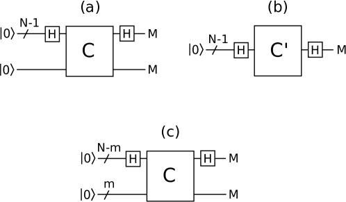
The Hadamard-classical circuit with one-qubit (HC1Q) model on qubits is the following quantum computing model (see Fig. 1(a)):
-
1.
The initial state is .
-
2.
is applied.
-
3.
A polynomial-time uniformly-generated classical reversible circuit
is applied “coherently”.
-
4.
is applied.
-
5.
All qubits are measured in the computational basis.
We show that the HC1Q model is universal with a postselection. More precisely, we show the following:
Theorem 3
Let be a polynomial-time uniformly-generated quantum circuit acting on qubits that consists of number of Hadamard gates and classical reversible gates, such as , CNOT, and Toffoli. Then from we can efficiently construct an HC1Q circuit on qubits such that a postselection on some output qubits generates the state .
Since Hadamard plus classical gates are universal, Theorem 3 shows that HC1Q model is universal with a postselection. A proof of the theorem is given in Sec. II. The proof is based on a new idea that is different from those used in the previous results TD ; BJS ; AA ; MFF . Proofs for the depth-four model TD , the Boson sampling model AA , and the IQP model BJS use gadgets that insert gates in a post hoc way by using postselections. (For example, the IQP model is not universal because Hadamard gates can be applied only in the first layer and the last layer, but the so-called Hadamard gadget BJS enables realizations of Hadamard gates in any place of the IQP model by using postselections.) The proof for the DQC1 model MFF uses a postselection to initialize the maximally-mixed state to the pure state . As is explained in Sec. II, our proof is different from those: from , we first construct a polynomial-time non-deterministic algorithm. From the polynomial-time non-deterministic algorithm, we next construct a classical deterministic polynomial-time circuit . We finally show that the HC1Q circuit can generate with a postselection. This idea itself seems to be useful for finding other new sub-universal models that exhibit quantum supremacy. We do not know relations between our technique and previous ones.
By using the arguments of Ref. BJS ; MFF ; AA , we obtain the following corollary of Theorem 3, which is quantum supremacy of the HC1Q model:
Corollary 4
Output probability distributions of the HC1Q model cannot be classically efficiently sampled within a multiplicative error unless the polynomial-time hierarchy collapses to the third level.
Here, we say that a probability distribution is classically efficiently sampled within a multiplicative error if there exists a classical probabilistic polynomial-time algorithm such that
for all , where is the probability that the algorithm outputs .
The corollary demonstrates an interesting “phase transition” between classical and quantum. To see it, let us consider the circuit of Fig. 1(b), which is obtained by removing the last qubit of the HC1Q model (Fig. 1(a)). Here,
is a polynomial-time uniformly-generated classical reversible circuit. The circuit of Fig. 1(b) is trivially classically simulatable, since is a permutation on and therefore
where . Our result therefore suggests that the addition of a single qubit to the trivial circuit of Fig. 1(b) changes its complexity dramatically.
The third level collapse of the polynomial-time hierarchy for the depth-four model, the Boson sampling model, the IQP model, and the DQC1 model can be improved to the second level collapse Kobayashi ; KobayashiICALP . In Sec. III, we show that the same improvement is possible for the HC1Q model:
Theorem 5
Output probability distributions of the HC1Q model cannot be classically efficiently sampled within a multiplicative error unless the polynomial-time hierarchy collapses to the second level.
A natural question is whether the above supremacy results still hold when the number of qubits measured is much reduced. It is known that for the -qubit IQP model probability distributions of measurement results on number of qubits can be classically exactly sampled in polynomial time BJS . In Sec. IV we show an analogous result for the HC1Q model:
Theorem 6
Probability distributions of measurement results on number of qubits in the HC1Q model can be classically sampled in polynomial time within a L1-norm error.
It is possible to extend this result to a generalized version of the HC1Q model, which we call the HCQ model:
Definition 7 (HCQ)
The Hadamard-classical circuit with -qubit (HCQ) model on qubits is the following quantum computing model (see Fig. 1(c)):
-
1.
The initial state is .
-
2.
is applied.
-
3.
A polynomial-time uniformly-generated classical reversible circuit
is applied “coherently”.
-
4.
is applied.
-
5.
All qubits are measured in the computational basis.
Theorem 8
Probability distributions of measurement results on number of qubits in the HCQ model can be classically sampled in polynomial time within a L1-norm error.
Its proof is omitted since it is similar to that of Theorem 6.
At this moment, we do not know which sub-universal model is the most promising for experimental realizations, but the HC1Q model should be useful for certain experimental setups due to its simple structure.
I.2 The verification of quantum computing in the second level of the Fourier hierarchy
In this paper, we also study the classical verification of quantum computing. It is a long-standing open problem whether quantum computing is classically verifiable. More precisely, it is open whether any problem in BQP has an interactive proof system with a quantum polynomial-time prover and a classical probabilistic polynomial-time verifier.
Definition 9
We say that a problem has an interactive proof system with a quantum polynomial-time prover if there exists a classical probabilistic polynomial-time verifier such that
-
•
If then there exists a quantum polynomial-time prover such that the verifier accepts with probability at least .
-
•
If then for any prover the verifier accepts with probability at most .
(Note that in this definition, the prover is in quantum polynomial-time only for yes instances, i.e., when the prover is honest. For no instances, the computational power of the malicious prover is unbounded.)
Answering the open question is important not only for practical applications of cloud quantum computing but also for foundations of computer science and quantum physics AharonovVazirani . In fact, several partial solutions to the open problem have been obtained. They are categorized into the following four types:
-
1.
Several verification protocols MNS ; posthoc and verifiable blind quantum computing protocols FK ; Aharonov ; HM ; Broadbent ; Andru_review demonstrate that if the verifier has a weak quantum ability, such as preparations or measurements of single-qubit quantum states, any BQP problem can be verified with a quantum polynomial-time prover.
- 2.
-
3.
Since BQP is contained in IP defIP , a natural approach to the open problem is to restrict the prover of IP to quantum polynomial-time when the problem is in BQP. In fact, recently, a step in this line has been obtained in Ref. AharonovGreen . The authors of Ref. AharonovGreen have constructed a new interactive proof system that verifies the value of the trace of operators with a postBQP prover and a classical polynomial-time verifier.
-
4.
It has been shown recently that the classical verification of quantum computing is possible if a certain problem is assumed to be hard for quantum computing Mahadev .
Actually, the answer to the open problem is unconditionally yes if we consider specific BQP problems. For example, it is known that the recursive Fourier sampling BV has an interactive proof system with a quantum polynomial-time prover and a classical polynomial-time verifier who communicate polynomial number of messages MattFourier . Furthermore, it has been shown recently that calculating orders of solvable groups has an interactive proof system with a quantum polynomial-time prover and a classical polynomial-time verifier who exchange two or three messages LeGall . Finally, it was suggested in Ref. Tommaso that a problem of deciding whether there exist some results that occur with high probability or not for circuits in FH2 has a Merlin-Arthur system with quantum polynomial-time Merlin.
Definition 10
We say that a problem has a Merlin-Arthur system with a quantum polynomial-time Merlin if has an interactive proof system with a quantum polynomial-time prover (Merlin) and a classical probabilistic polynomial-time verifier (Arthur) where only a single message transmission is done from the prover to the verifier.
The second main result of the present paper is to introduce another problem in BQP that is classically verifiable. More precisely, we define the following promise problem that we call Probability Distribution Distinguishability with Maximum Norm (PDD-Max):
Definition 11 (PDD-Max)
Given a classical description of two quantum circuits and acting on qubits that consist of number of elementary gates, and parameters and such that and , decide
-
•
YES: there exists such that .
-
•
NO: for any , .
Here, and .
We first show that PDD-Max exactly characterizes the power of BQP:
Theorem 12
PDD-Max is BQP-complete (under polynomial-time many-one reduction).
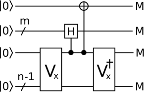
Its proof is given in Sec. V. (Note that if two circuits are classical, PDD-Max is BPP-complete; we have only to replace the controlled- gate in Fig. 3 with a controlled-random-bit-flip gate.)
We next show that if and of PDD-Max are restricted to the HC1Q model, PDD-Max is classically verifiable:
Theorem 13
If two circuits and are in the form of the HC1Q model, PDD-Max has a Merlin-Arthur system with quantum polynomial-time Merlin.
The proof of Theorem 13 is given in Sec. VI. A similar proof holds for the IQP model and the HCQ model (including the Simon-type circuits) (see Sec. VII.1).
These results demonstrate that if we restrict the circuits of PDD-Max to the form of the HC1Q model, it is another example of problems that is classically verifiable. These results also suggest that such a restriction of PDD-Max is not BQP-hard, since BQP is not believed to be in MA defMA .
The classical verifiability of PDD-Max for restricted circuits does not seem to be directly related to the classical verification of quantum supremacy, such as the verification of the IQP model, but it is an important future research subject to explore any relation between them.
I.3 Preliminary
In this paper, we often use the following well known inequality:
Theorem 14 (Chernoff-Hoeffding bound)
Let be identically and independently distributed real random variables with for every . Then
In the following sections, we give proofs of theorems. In the last section, Sec. VII, we provide some discussions.
II Proof of Theorem 3
In this section, we show Theorem 3. We are given a unitary operator
acting on qubits, where is the Hadamard gate or a classical gate for all . From , we define
where is acting on th qubit ().
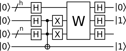
The outline of our proof is as follows. We first construct a polynomial-time non-deterministic algorithm from . We next define a polynomial-time quantum unitary operator , which consists of only classical gates, from the polynomial-time non-deterministic algorithm. We finally show that the HC1Q model of Fig. 2 that uses is universal with a postselection.
Now let us consider the following polynomial-time non-deterministic algorithm.
-
0.
The state of the register is represented by , where and .
-
1.
The initial state of the register is .
-
2.
Repeat the following for .
-
2-a.
If is a classical gate (such as , CNOT, or Toffoli) whose corresponding action on is
update the state of the register as
-
2-b.
If is acting on th qubit, update the state of the register in the following non-deterministic way:
-
2-a.
Let us define by
i.e., is the number of appearing in . The above polynomial-time non-deterministic algorithm does the non-deterministic transition times, and therefore the algorithm has computational paths. We label each path by an -bit string . We write the final state of the register for the path by , where and . Then, we obtain
| (2) |
(To help the readers understand the derivation of Eq. (2), we provide a simple example in Appendix A.)
Note that, for each , we can calculate and in classical polynomial-time. Let us define the polynomial-time unitary operator by
It is easy to see that can be constructed with only classical gates. Now we show that the state can be generated by the HC1Q model of Fig. 2 that uses with a postselection. In Fig. 2, the state immediately before the postselection is
| (3) |
where is a certain -qubit state whose detail is irrelevant keep . After the postselection, the state becomes
Hence, we have shown that the HC1Q model of Fig. 2 with a postselection can generate for any unitary that consists of Hadamard and classical gates, which means that the HC1Q model is universal with a postselection.
III Proof of Theorem 5
It was shown in Refs. Kobayashi ; KobayashiICALP that the third level collapse of the polynomial-time hierarchy for most of the sub-universal models (including the depth-four model TD , the Boson sampling model AA , the IQP model BJS , and the DQC1 model MFF ) is improved to the second level collapse. The idea is to use the class NQP NQP in stead of postBQP. NQP is a quantum version of NP, and defined as follows:
Definition 15 (NQP)
A promise problem is in NQP if and only if there exists a polynomial-time uniformly-generated family of quantum circuits such that if then , and if then . Here is the acceptance probability of .
If we remember the following definition of NP, it is clear that NQP is a quantum version of NP.
Definition 16 (NP)
A promise problem is in NP if and only if there exists a classical polynomial-time probabilistic algorithm such that if then , and if then . Here is the acceptance probability of the classical algorithm.
By using a similar argument of Refs. Kobayashi ; KobayashiICALP , we now show that the collapse of the polynomial-time hierarchy to the third level for the HC1Q model can be improved to the second level. Let be a promise problem in NQP. Then there exists a polynomial-time uniformly-generated family of quantum circuits that satisfies the above definition of NQP. The outline of our proof is as follows: First, from , we construct an HC1Q circuit. Second, we assume that its output probability distribution is classically efficiently sampled within a multiplicative error . Finally, we show that then is in NP, which means . It collapses the polynomial-time hierarchy to the second level, since
Now let us give a more precise proof. In Sec. II, we have constructed the HC1Q circuit of Fig. 2 from a given unitary . Let us repeat the same argument by replacing with . In stead of doing the postselection on the state of Eq. (3), let us do the projective measurement on it, where
The probability of obtaining is
By the definition of NQP,
when and
when . It means that when and when .
Assume that is classically efficiently sampled within a multiplicative error . It means that there exists a classical polynomial-time probabilistic algorithm that outputs or such that
where is the probability that the classical algorithm outputs 0 (accepts). Then, we can show that is in NP. In fact, if then
If then
According to Definition 16, is therefore in NP.
IV Proof of Theorem 6
In this section, we show Theorem 6. For simplicity, we assume that the first qubits are measured, where . Generalizations to other qubits are the same.
The outline of our proof is as follows. We first construct a probability distribution that can be calculated in classical polynomial time, and is close to within a L1-norm. We then show that we can sample in classical polynomial time.
Let us consider the circuit of Fig. 1 (a). As is shown in Appendix B, the probability of obtaining the measurement result for the first qubits is
| (4) |
where
is the first bits of , is the last bits of , and is defined by
The subset can be obtained in polynomial time in the following way:
-
1.
Set .
-
2.
Repeat the following for all .
-
2-1.
Calculate .
-
2-2.
If for certain , add to .
-
2-1.
-
3.
End.
From the construction, . Therefore, the value of is exactly computable in polynomial time for each . Furthermore, because
Let us generate random bit strings . We then calculate
Note that if we take , then , and therefore from the Chernoff-Hoeffding bound,
For any polynomial , let us take . Given , define the probability distribution by
Note that it is well defined, because
which is shown as follows:
Furthermore, is obtained in polynomial time. The distance between and is
It is shown as follows. First,
Second,
In this way, we have shown that we can calculate in classical polynomial time the probability distribution that is close to . Our final task is to show that can be sampled in classical polynomial time. For simplicity, let us assume that each is represented in the -bit binary:
where for . (Otherwise, by polynomially increasing the size of , we obtain exponentially good approximations.) The following algorithm samples the probability distribution .
-
1.
Randomly generate an -bit string .
-
2.
Output such that
where and mean the standard dictionary order. (For example, for three bits, .)
In summary, we have shown that can be sampled in polynomial time within a L1-norm error.
V Proof of Theorem 12
In this section, we show Theorem 12. Our proof consists of two parts. In the first subsection, we show that PDD-Max is BQP-hard. In the second subsection, we show that PDD-Max is in BQP.
V.1 BQP-hardness
Let be a promise problem in BQP. It means that there exists a uniform family of polynomial-size quantum circuits such that if then accepts with probability at least , and if then accepts with probability at most , where is any polynomial. More precisely, let be the polynomial-size quantum circuit, which acts on qubits, corresponding to the instance . If we write as
with certain -qubit states and , we have when , and when . Let us consider the circuit of Fig. 3. We call it . We also define
We now show that deciding or can be reduced to a PDD-Max problem with and , which means that PDD-Max is BQP-hard. In fact, note that
Let be the probability that we obtain when we measure all qubits of in the computational basis. When ,
When ,
for any . Let , where . Since , it is obvious that for any . Therefore, when ,
and when ,
for any . In this way, we have shown that PDD-Max is BQP-hard.
V.2 In BQP
We next show that PDD-Max is in BQP. We show that the following BQP algorithm solves PDD-Max with a completeness-soundness gap (i.e., the gap of acceptance probabilities between the yes-instances and the no-instances is lowerbounded by ):
-
1.
Flip a fair coin . Generate , and measure each qubit in the computational basis. Let be the measurement result.
-
2.
Repeat the following for , where is a polynomial of specified later.
-
2-a.
Generate , and measure all qubits in the computational basis. If the result is , then set . Otherwise, set .
-
2-a.
-
3.
Calculate
Note that , where . Therefore, from the Chernoff-Hoeffding bound, with probability larger than . In a similar way, calculate the estimator of . From the Chernoff-Hoeffding bound, with probability larger than .
-
4.
Calculate . If , accept. Otherwise, reject.
The intuitive idea of this algorithm is as follows. By the definition of the PDD-Max, if the answer of the PDD-Max is yes, there exists such that is large. In this case, the probability of obtaining such in step 1 is large. Therefore let us assume that we obtain such in step 1. The step 1 is, in other words, the process to find a candidate of the solution. In steps 2 and 3, probabilities and are estimated by using the Chernoff-Hoeffding bound. Finally, in step 4, we check whether is indeed large, and accept with high probability since it is actually large. If the answer of the PDD-Max is no, on the other hand, there is no such that is large, and therefore in step 4 we do not conclude that is large except for some failure probability. (Note that for general and , estimating and seems to require BQP power, since it seems to be necessary to generate and . We will see in the next section that if and are restricted in FH2, the estimation of and can be done in classical polynomial time, and therefore PDD-Max has a Merlin-Arthur system with quantum polynomial-time Merlin.)
Now let us give a more precise proof that PDD-Max is in BQP. First, let us consider the case when the answer to PDD-Max is YES. If obtained in step 1 satisfies , and if and calculated in steps 2 and 3 satisfy and , we definitely accept in step 4, because
and therefore
The probability of occurring such an event is calculated to be
where we have taken and is any polynomial of . Therefore, the acceptance probability of our protocol is lowerbounded as
Next, let us consider the case when the answer to PDD-Max is NO. If and , which occurs with probability , we definitely reject, because
The rejection probability is therefore lowerbounded as
Therefore, the acceptance probability is upperbounded as
The completeness-soundness gap is therefore
for sufficiently large , which shows that PDD-Max is in BQP.
VI Proof of Theorem 13
In this section, we show Theorem 13. Before giving the proof, let us explain the intuitive idea. In Sec. V.2, we have seen that PDD-Max is in BQP for general and . In step 1 of the algorithm, a candidate of the solution, i.e., such that , is obtained by doing quantum computing. In step 2, another quantum computing is necessary to estimate and . In the following we will see that if and are the HC1Q model, estimations of and can be done in classical polynomial-time. Therefore, we can construct the following Merlin-Arthur protocol with quantum polynomial-time Merlin:
-
1.
Merlin does the step 1 of the protocol in Sec. V.2, i.e., Merlin generates and sends it to Arthur.
-
2.
Arthur verifies is large.
Now let us show Theorem 13. Our Merlin-Arthur protocol with quantum polynomial-time Merlin runs as follows.
-
1.
If Merlin is honest, he flips a fair coin . He next generates , and measures each qubit in the computational basis to obtain the result . He sends to Arthur. If Merlin is malicious, his computational ability is unbounded, and what he sends to Arthur can be any bit string.
-
2.
Let be a polynomial of specified later. Arthur generates and , where each of and is a uniformly and independently chosen random bit string.
-
3.
Arthur calculates
where
Here,
is the classical circuit in ,
is the th bit of , and is the th bit of . We call the estimator of . Note that can be calculated in classical time.
-
4.
In a similar way, Arthur calculates the estimator of . If
Arthur accepts. Otherwise, he rejects.
Note that
| (5) |
Its derivation is given in Appendix C. If we set , we have
Therefore, from the Chernoff-Hoeffding bound, the estimator satisfies with probability . For , a similar result holds. In the above protocol, the honest prover is enough to be quantum polynomial-time.
Now we show that the above protocol can verify PDD-Max. The proof is similar to that for the BQP case given in Sec. V. First, let us consider the case when the answer to PDD-Max is yes. If the that Merlin sends to Arthur satisfies , and the estimators and that Arthur calculates satisfy and , Arthur definitely accepts, because
Taking the honest prover in step 1, the probability of occurring such an event is calculated to be
where we have taken and is any polynomial of . Therefore, the probability that Arthur accepts in our protocol is lowerbounded as
Next, let us consider the case when the answer to PDD-Max is no. If and , which occurs with probability , Arthur definitely rejects, because
Therefore, the probability that Arthur accepts in our protocol is upperbounded as
The completeness-soundness gap is therefore
for sufficiently large , which shows that PDD-Max has a Merlin-Arthur system with quantum polynomial-time Merlin.
Remarks. To conclude this section, we provide some remarks. Note that the fact that and can be estimated in classical polynomial-time seems to be a special property only for some circuits (such as those in FH2), and we do not know how to do that for other general circuits. (In particular, in Sec. VII.2, we will explain why the technique we use for FH2 circuits will not work for other circuits, such as FH3 circuits.) Furthermore, note that what Arthur can do is to estimate within an additive error given : he cannot sample . (If he can do it, he can solve factoring and Simon’s problem, for example.)
VII Discussion
VII.1 Generalizations to other circuits
In the proof of Theorem 13 (Sec. VI), we have considered the HC1Q model. Similar proofs hold for other circuits in FH2. For example, let us consider the IQP model. For the IQP model, is a complex-valued function, but we can use the Chernoff-Hoeffding bound for complex random variables introduced in Ref. NestSchwarz .
The other example is the HCQ model. We can show a similar result for it. In fact, the probability of obtaining the result is
and therefore the Chernoff-Hoeffding bound argument can be used. Here, is the first bits of , and is the last bits of .
Furthermore, we would like to point out that PDD-Max can has a Merlin-Arthur system with quantum polynomial-time Merlin for other circuits outside of FH2. The essential point of our proof is that the output probability distributions, and , of and can be classically efficiently estimated. This property itself is not restricted to circuits in FH2, and therefore we believe that our results should hold for many other circuits outside of FH2.
VII.2 FH3
FH2 circuits have nice structures such that and can be estimated in classical polynomial-time. We do not know how to do the same thing for other circuits such as those in FH3. The reason is as follows. From a similar calculation given in Appendix C, we can show that the probability for an FH3 circuit satisfies
for certain and a certain function . However, in this case, we no longer have , but is exponentially increasing as a function of : , where and is a polynomial. Then, by using the Chernoff-Hoeffding bound, we can obtain an estimator that satisfies
with probability larger than . The above inequality means
which also means
In order to make , must be exponentially small, which means that must be exponentially large. Therefore, we cannot obtain a -precision estimator of in classical polynomial time. Note that it is known that as long as we use as a black box, the Chernoff-Hoeffding type bounds are optimal (up to some factors) Canetti . This is the reason why our previous proof does not work for other circuits.
Acknowledgements.
We thank Keisuke Fujii, Seiichiro Tani, and Francois Le Gall for discussion. TM is supported by JST ACT-I No.JPMJPR16UP, JST PRESTO, and the Grant-in-Aid for Young Scientists (B) No.JP17K12637 of JSPS. YT is supported by the Program for Leading Graduate Schools: Interactive Materials Science Cadet Program and JSPS Grant-in-Aid for JSPS Research Fellow No.JP17J03503. HN is supported by the Grant-in-Aid for Scientific Research (A) Nos.26247016, 16H01705 and (C) No.16K00015 of JSPS.Appendix A Example
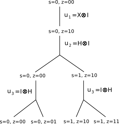
Let us consider the simple example where , , and . In this case, , where
The computational tree that represents the non-deterministic algorithm corresponding to is given in Fig. 4. Each Hadamard gate in corresponds to a non-deterministic transition. The bit string represents a basis state, and the bit represents the sign of a basis state. If we superpose for all computational path , we obtain
Appendix B Derivation of Eq. (4)
Appendix C Derivation of Eq. (5)
References
- (1) Y. Shi, Quantum and classical tradeoffs. Theoretical Computer Science 344, 335 (2005). DOI:10.1016/j.tcs.2005.03.053
- (2) D. R. Simon, On the power of quantum computation. Proceedings of the 35th Annual Symposium on Foundations of Computer Science (FOCS 1994), p.116 (1994). DOI:10.1137/S0097539796298637
- (3) P. Shor, Algorithms for quantum computation: discrete logarithms and factoring. Proceedings of the 35th Annual Symposium on Foundations of Computer Science (FOCS 1994), p.124 (1994). DOI:10.1109/SFCS.1994.365700
- (4) M. J. Bremner, R. Jozsa, and D. J. Shepherd, Classical simulation of commuting quantum computations implies collapse of the polynomial hierarchy. Proc. R. Soc. A 467, 459 (2011). DOI:10.1098/rspa.2010.0301
- (5) M. J. Bremner, A. Montanaro, and D. J. Shepherd, Average-case complexity versus approximate simulation of commuting quantum computations. Phys. Rev. Lett. 117, 080501 (2016). DOI:10.1103/PhysRevLett.117.080501
- (6) B. M. Terhal and D. P. DiVincenzo, Adaptive quantum computation, constant depth quantum circuits and Arthur-Merlin games. Quant. Inf. Comput. 4, 134 (2004). DOI:10.26421/QIC4.2
- (7) S. Aaronson and A. Arkhipov, The computational complexity of linear optics. Theory of Computing 9, 143 (2013). DOI:10.1145/1993636.1993682
- (8) E. Knill, and R. Laflamme, Power of one bit of quantum information. Phys. Rev. Lett. 81, 5672 (1998). DOI:10.1103/PhysRevLett.81.5672
- (9) T. Morimae, K. Fujii, and J. F. Fitzsimons, Hardness of classically simulating the one clean qubit model. Phys. Rev. Lett. 112, 130502 (2014). DOI:10.1103/PhysRevLett.112.130502
- (10) T. Morimae, Hardness of classically sampling one clean qubit model with constant total variation distance error. Phys. Rev. A 96, 040302(R) (2017). DOI:10.1103/PhysRevA.96.040302
- (11) K. Fujii, H. Kobayashi, T. Morimae, H. Nishimura, S. Tamate, and S. Tani, Impossibility of classically simulating one-clean-qubit computation. Phys. Rev. Lett. 120, 200502 (2018). DOI:10.1103/PhysRevLett.120.200502
- (12) K. Fujii, H. Kobayashi, T. Morimae, H. Nishimura, S. Tamate, and S. Tani, Power of quantum computation with few clean qubits. Proceedings of 43rd International Colloquium on Automata, Languages, and Programming (ICALP 2016), p.13:1. DOI:10.4230/LIPIcs.ICALP.2016.13
- (13) B. Fefferman and C. Umans, The power of quantum Fourier sampling. arXiv:1507.05592
- (14) A. Bouland, J. F. Fitzsimons, and D. E. Koh, Quantum advantage from conjugated Clifford circuits. Proceedings of the 33rd Computational Complexity Conference (CCC2018). DOI:10.4230/LIPIcs.CCC.2018.21
- (15) A. Bouland, B. Fefferman, C. Nirkhe, and U. Vazirani, On the complexity and verification of quantum random circuit sampling. Nat. Phys. 2018 DOI:10.1038/s41567-018-0318-2
- (16) D. Aharonov and U. Vazirani, Is quantum mechanics falsifiable? A computational perspective on the foundations of quantum mechanics. arXiv:1206.3686
- (17) T. Morimae, D. Nagaj, and N. Schuch, Quantum proofs can be verified using only single-qubit measurements. Phys. Rev. A 93, 022326 (2016). DOI:10.1103/PhysRevA.93.022326
- (18) J. F. Fitzsimons, M. Hajdušek, and T. Morimae, Post hoc verification of quantum computation. Phys. Rev. Lett. 120, 040501 (2018). DOI:10.1103/PhysRevLett.120.040501
- (19) J. F. Fitzsimons and E. Kashefi, Unconditionally verifiable blind computation. Phys. Rev. A 96, 012303 (2017). DOI:10.1103/PhysRevA.96.012303
- (20) D. Aharonov, M. Ben-Or, E. Eban, and U. Mahadev, Interactive proofs for quantum computations. arXiv:1704.04487
- (21) M. Hayashi and T. Morimae, Verifiable measurement-only blind quantum computing with stabilizer testing. Phys. Rev. Lett. 115, 220502 (2015). DOI:10.1103/PhysRevLett.115.220502
- (22) A. Broadbent, How to verify quantum computation. Theory of Computing 14, 1 (2018). DOI:10.4086/toc.2018.v014a011
- (23) A. Gheorghiu, T. Kapourniotis, and E. Kashefi, Verification of quantum computation: an overview of existing approaches. arXiv:1709.06984
- (24) M. McKague, Interactive proofs for BQP via self-tested graph states. Theory of Computing 12, 1 (2016). DOI:10.4086/toc.2016.v012a003
- (25) Z. Ji, Classical verification of quantum proofs. Proceedings of the 48th annual ACM symposium on Theory of Computing (STOC 2016) p.885 (2016). DOI:10.1145/2897518.2897634
- (26) B. W. Reichardt, F. Unger, and U. Vazirani, Classical command of quantum systems. Nature 496, 456 (2013). DOI:10.1038/nature12035
- (27) IP is the class of promise problems verified by an interactive proof system with a BPP verifier and a prover with unlimited computational ability.
- (28) D. Aharonov and A. Green, A quantum inspired proof of . arXiv:1710.09078
- (29) U. Mahadev, Classical verification of quantum computations. arXiv:1804.01082
- (30) E. Bernstein and U. Vazirani, Quantum complexity theory. SIAM Journal on Computing 26, 1411 (1997). DOI:10.1137/S0097539796300921
- (31) M. McKague, Interactive proofs with efficient quantum prover for recursive Fourier sampling. Chicago Journal of Theoretical Computer Science 6, 1 (2012). DOI:10.4086/cjtcs.0006
- (32) T. F. Demarie, Y. Ouyang, and J. F. Fitzsimons, Classical verification of quantum circuits containing few basis changes. Phys. Rev. A 97, 042319 (2018). DOI:10.1103/PhysRevA.97.042319
- (33) F. Le Gall, T. Morimae, H. Nishimura, and Y. Takeuchi, Interactive proofs with polynomial-time quantum prover for computing the order of solvable groups. arXiv:1805.03385
- (34) Merlin-Arthur (MA) is the class of promise problems that can be verified by a BPP verifier and a prover whose computational ability is unlimited. In MA, the prover first sends a bit string to the verifier, and the verifier then does the computing for the verification.
- (35) Note that the -qubit Toffoli gate in Fig. 2 can be implemented with a polynomially many Toffoli gates by using ancilla qubits Barenco . It is known that ancilla qubits do not need to be initialized Barenco . Therefore, we can use states as ancilla qubits, which keeps the circuit of Fig. 2 in the form of Fig. 1(a).
- (36) A. Barenco, C. H. Bennett, R. Cleve, D. P. DiVincenzo, N. Margolus, P. Shor, T. Sleator, J. A. Smolin, H. Weinfurter, Elementary gates for quantum computation. Phys. Rev. A 52 3457 (1995). DOI:10.1103/PhysRevA.52.3457
- (37) L. M. Adleman, J. DeMarrais, and M. A. Huang, Quantum Computability. SIAM J. Comput. 26 1524 (1997). DOI:10.1137/S0097539795293639
- (38) M. Schwarz and M. Van den Nest, Simulating quantum circuits with sparse output distributions. arXiv:1310.6749
- (39) R. Canetti, G. Even, and O. Goldreich, Lower bounds for sampling algorithms for estimating the average. Information Processing Letters 53, 17 (1995).
