Theory of long range interactions for Rydberg states attached to hyperfine split cores

Abstract

The theory is developed for one and two atom interactions when the atom has a Rydberg electron attached to a hyperfine split core state. This situation is relevant for some of the rare earth and alkaline earth atoms that have been proposed for experiments on Rydberg-Rydberg interactions. For the rare earth atoms, the core electrons can have a very substantial total angular momentum, $J$, and a non-zero nuclear spin, $I$. In the alkaline earth atoms there is a single, $s$, core electron whose spin can couple to a non-zero nuclear spin for odd isotopes. The resulting hyperfine splitting of the core state can lead to substantial mixing between the Rydberg series attached to different thresholds. Compared to the unperturbed Rydberg series of the alkali atoms, the series perturbations and near degeneracies from the different parity states could lead to qualitatively different behavior for single atom Rydberg properties (polarizability, Zeeman mixing and splitting, etc) as well as Rydberg-Rydberg interactions ($C_{5}$ and $C_{6}$ matrices).

I Introduction

The structure and interactions of atoms excited to Rydberg states have been intensively studied for many years. Detailed experimental measurements of Rydberg properties were initially performed with alkali and alkaline earth atomsGallagher (1994). More recently there has been a growing interest in the use of rare earth atoms, primarily lanthanides, for experiments with degenerate quantum gasesLu et al. (2011, 2012); Aikawa et al. (2012); Frisch et al. (2014); Schmitt et al. (2016), and for quantum informationSaffman and Mølmer (2008). Alkaline earth atoms are also the subject of increased interest for quantum information applicationsDaley et al. (2008); Shibata et al. (2009). The availability of Rydberg state mediated potentials provides a tunable experimental control parameter for studies of long range interactions and entanglement. Several works have proposed incorporating Rydberg interactions in experiments with alkaline earthMukherjee et al. (2011); Topcu and Derevianko (2014, 2016); Gil et al. (2014); Khazali et al. (2016) and lanthanideSaffman and Mølmer (2008) atoms.

The Rydberg structure of these multi-electron atoms is substantially more complex than for single electron alkali atoms. The standard theoretical technique used to quantitatively describe these atoms is multichannel quantum defect theory (MQDT) as presented, for example, in Ref. Aymar et al. (1996). Several recent works have used MQDT to calculate the interaction potentials between Rydberg excited alkaline earth atomsVaillant et al. (2012, 2014). The combination of multiple Rydberg series and a hyperfine split core state can lead to mixing between Rydberg series attached to different thresholds leading to additional complexity. Hyperfine structure is present in alkaline earth and lanthanide isotopes with an odd number of nucleons and thereby a nonzero nuclear spin. These isotopes are listed in Tables 1, 2. Relatively few experiments have reported on the hyperfine structure of these complex atomsRinneberg and Neukammer (1982, 1983); Eliel and Hogervorst (1983); Aymar (1984a); Beigang et al. (1983); Nörtershäuser et al. (2000); Jin et al. (2011).

isotope	nuclear spin	Rydberg spectroscopy experiments
9Be	$3/2$	Ray et al. (1988); Yoshida et al. (2006)
25Mg	$5/2$	Beigang and Schmidt (1981); Wehlitz et al. (2007)
43Ca	$7/2$	Beigang et al. (1982); Gentile et al. (1990)
87Sr	$9/2$	Cooke et al. (1978); Beigang et al. (1983); Mauger et al. (2007)
135Ba, 137Ba	$3/2$	Rinneberg and Neukammer (1982, 1983); Eliel and Hogervorst (1983); Aymar (1984a)

Table 1: Stable alkaline earth isotopes with hyperfine structure. There have been a large number of measurements of the Rydberg spectra of alkaline earth atoms. The cited references are representative and not intended to be complete.

The Rydberg structure of multielectron atoms with hyperfine split cores has been only partially dealt with in earlier theoretical worksAymar (1984b, a); Sun and Lu (1988); Sun (1989); Aymar et al. (1996); Sun et al. (1989). These studies focused on obtaining the energies for bound and autoionizing states as well as the dipole transition operator from the ground or low-lying excited states. The objective of this paper is to develop a detailed formalism that can be applied for calculation of single atom Rydberg properties and two-atom interaction strengths. In addition to the energies and dipole transition operators, we provide a framework to calculate the Zeeman shift and coupling as well as the Stark shift and coupling between Rydberg states for atoms in weak magnetic and electric fields. In addition to one atom properties, we describe a formalism for obtaining the $C_{n}$ coefficients for the Rydberg-Rydberg interactions and provide specific formulas for the $C_{5}$ and $C_{6}$ matrices. The calculation of these interaction matrices has not been discussed for Rydberg states attached to hyperfine split thresholds.

The rest of the paper is organized as follows. Section II contains the basic ideas for the frame transformations which form the foundation for the rest of the developments. The frame transformation for hyperfine split core states has been developed and has been applied several times in experimentsSun and Lu (1988); Sun (1989); Sun et al. (1989); Wörner et al. (2003); Schäfer and Merkt (2006); Schäfer et al. (2010). The inclusion of the frame transformation is for completeness and to specify the notation used in the rest of this paper. Section II goes beyond the previous developments by giving the expressions for the Zeeman and Stark effect for Rydberg states attached to hyperfine split core states. Section III includes the derivation for Rydberg-Rydberg interactions with specific derivation of the $C_{5}$ and $C_{6}$ matrices. Section IV gives the parameters that are known for ¹⁶⁵Ho which will be used in example calculations. Sections V and VI give example results for the one atom and two atom interactions for ¹⁶⁵Ho. Because the Rydberg properties of Ho are only partially known, these calculations are presented more to demonstrate how to use the theory than for the specific results. This is followed by a short summary.

isotope	nuclear spin	Rydberg spectroscopy experiments
159La	$7/2$	Xue et al. (1997); Sun et al. (2001)
141Pr	$5/2$
143Nd, 145Nd	$7/2$
149Sm	$7/2$	Jayasekharan et al. (2000); Wen-Jie et al. (2009); Zhao et al. (2011); Shah et al. (2014)
151Eu, 153Eu	$5/2$	Nakhate et al. (2000); Xie et al. (2011); Bhattacharyya et al. (2007); Wang et al. (2012)
155Gd, 157Gd	$3/2$	Miyabe et al. (1998); Nörtershäuser et al. (2000); Jin et al. (2011); Ankush and Deo (2013)
159Tb	$3/2$
161Dy, 163Dy	$5/2$	Xu et al. (1992); Studer et al. (2016)
165Ho	$7/2$	Hostetter et al. (2015)
167Er	$7/2$
169Tm	$1/2$	Vidolova-Angelova et al. (1989)
171Yb, 173Yb	$1/2,\leavevmode\nobreak\ 5/2$	Camus et al. (1980); Aymar et al. (1984); Ali et al. (1999); Zinkstok et al. (2002)
175Lu	$7/2$	Ogawa and Kujirai (1999); Dai et al. (2003); Li et al. (2017a)

Table 2: Stable or observationally stable lanthanide isotopes with hyperfine structure. Measurements of the ionization potentials for all the lanthanides can be found inWorden et al. (1978). The cited references are representative and not intended to be complete.

Atomic units are used unless explicitly stated otherwise.

II One atom theory

To organize the thinking about this type of system, we will first consider how to describe the single atom Rydberg series. Also, most of the expressions for matrix elements for Rydberg-Rydberg systems are present in the one atom theory. One of the difficulties is to keep track of all of the quantum numbers. In this section, we will use the symbol $\alpha_{c}$ to indicate all of the quantum numbers in the core state except the hyperfine angular momentum $F_{c}$. The Rydberg electron quantum numbers will be denoted $n,s,\ell,j$ for the principal quantum number, spin, orbital angular momentum and total angular momentum.

One can get an idea of the principal quantum number where perturbers attached to different hyperfine levels start to perturb each other by setting the spacing of Rydberg energies, $1/\nu^{3}$, equal to the spacing of the hyperfine energies $\Delta E_{c}$. The parameter $\nu=n-\mu$ where $\mu$ is the quantum defect and $n$ is the principal quantum number. For a 10 GHz spacing, $\Delta E_{c}=1.52\times 10^{-6}$ atomic units (a.u.) which corresponds to $\nu\simeq 87$. In the rare earth positive ions, the splitting of the ionization thresholds can be larger than this which means the interactions between channels can be at smaller $\nu$. As an example, taking the Ho⁺ $F_{c}=23/2$ state as $E=0$, the $21/2$ state is at $-$17.6 GHz, the 19/2 state is at $-$34.0 GHz, the 17/2 state is at $-$48.9 GHz, etc.Lawler et al. (2004)

II.1 Bound states

In this subsection, we will review the idea for how to find the bound states and normalize themAymar et al. (1996). For a Rydberg electron attached to channel $|\Phi_{i}\rangle$, the coupled, real functions $|\psi_{i}\rangle$ with unphysical boundary conditions at large $r$ can be written as

$$|\psi_{i}\rangle=\sum_{i^{\prime}}|\Phi_{i^{\prime}}\rangle(f_{i^{\prime}}(r)\delta_{i^{\prime},i}-g_{i^{\prime}}(r)K_{i^{\prime},i})$$ (1)

where the $f,g$ are the energy normalized, radial Coulomb functions which are regular,irregular at the origin and ${\bf K}$ is the real, symmetric K-matrix. The Coulomb functions $f_{i^{\prime}},g_{i^{\prime}}$ are for an orbital angular momentum $\ell_{i^{\prime}}$ and at energy $E-E_{c,i^{\prime}}$ with $E$ being the total energy and $E_{c,i^{\prime}}$ is the energy of the core state $|\Phi_{i^{\prime}}\rangle$ which encompasses all of the degrees of freedom except the radial coordinate of the Rydberg electron. The $|\psi_{i}\rangle$ function is unphysical because the $f_{i^{\prime}},g_{i^{\prime}}$ functions diverge at large $r$ for closed channels defined by $E<E_{c,i^{\prime}}$. It is understood that this form only holds when the Rydberg electron is at distances, $r$, larger than the radial size of the core state. The K-matrix parameterizes the coupling between the $N$ different channels. At large distances, the $f,g$ vary rapidly with energy while the K-matrix will be assumed to not vary rapidly with energy. When the total energy is less than the threshold energy for all channels, the $N$ different $|\psi_{i}\rangle$ can not be superposed in a way to remove the exponential divergence at large $r$ for the Rydberg electron unless the total energy is at one of the bound state energies. Both of the $f,g$ functions diverge as $r\to\infty$ with

$$\lim_{r\to\infty}f_{i^{\prime}}(r)/g_{i^{\prime}}(r)\to-\tan(\beta_{i^{\prime}})$$ (2)

with $\beta_{i^{\prime}}=\pi(\nu_{i^{\prime}}-\ell_{i^{\prime}})$ and the effective quantum number defined by $E=E_{c,i^{\prime}}-1/[2\nu_{i^{\prime}}^{2}]$ with $E$ being the total energy and $E_{c,i^{\prime}}$ is the energy of the $i^{\prime}$-th core state.

At a bound state energy, $E_{b}$, the $|\psi_{i}\rangle$ can be superposed so that the exponentially diverging parts of the wave function all cancel perfectly. This only leaves radial functions that exponentially converge to 0 as $r\to\infty$. The superposition coefficients are defined as

$$|\psi_{b}\rangle=\sum_{i}|\psi_{i}\rangle\frac{\cos(\beta_{i})}{\nu_{i}^{3/2}}A_{i,b}$$ (3)

and the condition that determines them isAymar et al. (1996)

$$\sum_{i}(\tan(\beta_{i^{\prime}})\delta_{i^{\prime},i}+K_{i^{\prime},i})\frac{\cos(\beta_{i})}{\nu_{i}^{3/2}}A_{i,b}=0.$$ (4)

This condition can be satisfied only for the energies where the determinant of the term in parenthesis, $\tan\beta+K$, is zero. When this condition is satisfied, the bound state function can be written as

$$|\psi_{b}\rangle=\sum_{i}|\Phi_{i}\rangle P_{\nu_{i}\ell_{i}}(r)A_{i,b}$$ (5)

where the radial Coulomb function that goes to 0 at infinity is

$$P_{\nu_{i}\ell_{i}}(r)=(f_{i}\cos(\beta_{i})+g_{i}\sin(\beta_{i}))/\nu_{i}^{3/2}.$$ (6)

In the limit that the K-matrix is slowly varying as a function of principal quantum number (typically true for weakly bound Rydberg states), the normalization condition is

$$\sum_{i}A^{2}_{i,b}=1$$ (7)

which, with Eq. (4), defines the $A_{i,b}$ within an irrelevant, overall sign.

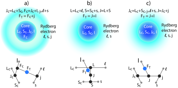
Figure 1: A schematic showing the different angular momentum coupling schemes for the frame transformations. The coupling in a) is appropriate when the Rydberg electron is in the far outer region, $|{\rm out}\rangle$. The coupling in b) is appropriate when all of the electrons are in the core region, $|{\rm in}^{(LS)}\rangle$. The coupling in c) is appropriate when the Rydberg is just outside of the core region but is not at sufficient distance for the hyperfine interaction to give important phase differences in the Coulomb functions, $|{\rm in}^{(jj)^{\prime}}\rangle$.

II.2 Frame transformation

Since the K-matrix is real and symmetric, there are $N(N-1)/2$ parameters for the coupling of the channels. Unfortunately, it is well beyond current computational resources to calculate the K-matrix with sufficient accuracy to be useful for the lanthanides, for example. The experimental energies for the bound states can be measured very accurately and constrain the values of the K-matrix. Because we assume the K-matrix has little variation with energy, the many different energies for the bound states can lead to the case of having more energies than unknown values in ${\bf K}$. However, for complex atoms, the number of different free parameters can be large which makes the fitting process itself a difficult numerical problem.

One solution is to use frame transformation ideas to limit the number of free parameters to $\sim N$.Aymar et al. (1996) The frame transformation for a hyperfine split core state was developed in Ref. Sun (1989) and applied to the hyperfine states of odd isotopes of SrSun et al. (1989) or the hyperfine states of the heavier noble gas atoms.Wörner et al. (2003); Schäfer and Merkt (2006); Schäfer et al. (2010) There are several different ways for coupling the angular momentum to obtain a frame transformation. The derivation in this section describes the method we used.

The angular momentum coupling we used when the Rydberg electron is in the outer region, Fig. 1a), couples the total spin, $S_{c}$, and orbital angular momentum, $L_{c}$, of the core to give a total angular momentum of the core, $J_{c}$, which is coupled to the nuclear spin, $I$, to give the hyperfine angular momentum of the core, $F_{c}$. The Rydberg electron has its spin, $s$, and orbital angular momentum, $\ell$, coupled together to give a total angular momentum, $j$. The total angular momentum of the core is coupled to the total angular momentum of the Rydberg electron to give the total angular momentum, $F_{T}$. We will symbolically write this coupling scheme as

$$|{\rm out}\rangle=|(((S_{c}L_{c})J_{c}I)F_{c}(s\ell)j)F_{T}\rangle$$ (8)

with the ordering of the parenthesis indicating which angular momenta are being coupled at each stage.

When the Rydberg electron is at short distances, then the LS-coupling is more appropriate, Fig. 1b). Within this scheme, the total spin of the core is coupled to the spin of the Rydberg electron to give the total spin, $S$, the total orbital angular momentum of the core is coupled to the orbital angular momentum of the Rydberg electron to give the total orbital angular momentum, $L$. The total spin and total orbital angular momentum are coupled to give the total angular momentum of all electrons, $J$, which is then coupled to the spin of the nucleus to give the total angular momentum, $F_{T}$. We will symbolically write this coupling scheme as

$$|{\rm in}^{(LS)}\rangle=|(((S_{c}s)S(L_{c}\ell)L)JI)F_{T}\rangle.$$ (9)

Typically, the frame transformation would obtain the K-matrix in the $|{\rm out}\rangle$ states by projecting onto the $|{\rm in}^{(LS)}\rangle$ states. However, it seems likely that higher accuracy will be needed. So we will adopt a method where there will be an intermediate jj-coupling, Fig. 1c). This coupling will be to couple the spin of the core electrons to the orbital angular momentum of the core electrons to obtain the total electronic angular momentum of the core, $J_{c}$, and similarly for the Rydberg electron giving its total angular momentum, $j$. These two angular momenta are coupled together to give the total angular momentum of the electrons, $J$, which is coupled to the spin of the nucleus to give the total angular momentum of the atom. This will be represented as

$$|{\rm in}^{(jj)}\rangle=|(((S_{c}L_{c})J_{c}(s\ell)j)JI)F_{T}\rangle.$$ (10)

By using this coupling, we can use the LS-coupled K-matrix to obtain a jj-coupled K-matrix using a frame transformation. The advantage of this intermediate step is that the resulting jj-coupled K-matrix can be corrected as discussed in Sec. II.2.1.

The unitary matrix that arises from this step of the frame transformation is

$$\langle{\rm in}^{(LS)}|{\rm in}^{(jj)}\rangle = \langle((S_{c}s)S(L_{c}\ell)L)J|((S_{c}L_{c})J_{c}(s\ell)j)J\rangle$$ (11)

$$= [S,L,J_{c}j]\begin{Bmatrix}S_{c}&s&S\\ L_{c}&\ell&L\\ J_{c}&j&J\end{Bmatrix}$$

which is from Eq. (6.4.2) of Ref. Edmonds (1974). The notation $[a,b,...]=\sqrt{(2a+1)(2b+1)...}$ and the $I$ and $F_{T}$ quantum numbers drop out because they are in the same spot in the bra and in the ket.

The frame transformation approximation assumes that the channel coupling between different $|{\rm in}^{(LS)}\rangle$ channels is small because LS-coupling dominates the interaction. In this case the, K-matrix in jj-coupling is approximated as

$$K^{(jj)}_{aa^{\prime}}=\sum_{LS}\langle{\rm in}^{(jj)}_{a}|{\rm in}^{(LS)}\rangle K^{(LS)}\langle{\rm in}^{(LS)}|{\rm in}^{(jj)}_{a^{\prime}}\rangle$$ (12)

where $K^{(LS)}=\tan[\pi\mu(LS)]$. For this expression, there is a sum over all LS-coupled channels that satisfy the angular momentum relations. The parameters $a,a^{\prime}$ are indicating the different jj-coupled channels

The jj-coupled K-matrices are then frame transformed to the $|{\rm out}\rangle$ channels using the projection matrix

$$\langle{\rm in}^{(jj)}|{\rm out}\rangle=\langle((J_{c}j)JI)F_{T}|((J_{c}I)F_{c}j)F_{T}\rangle$$

$$=(-1)^{3j+F_{c}+2J_{c}+I-J}[J,F_{c}]\begin{Bmatrix}j&J_{c}&J\\ I&F_{T}&F_{c}\end{Bmatrix}$$ (13)

where the last step used Eq. (6.1.5) of Ref. Edmonds (1974) and the earlier steps use $\langle j_{1}m_{1},j_{2}m_{2}|j_{12}m_{12}\rangle=(-1)^{j_{1}+j_{2}-j_{12}}\langle j_{2}m_{2},j_{1}m_{1}|j_{12}m_{12}\rangle$. We have checked that the resulting expression for the composite $\langle{\rm in}|{\rm out}\rangle$ gives a unitary matrix. The K-matrix in the channels $|{\rm out}\rangle$ is obtained by a frame transformation

$$K_{i^{\prime},i}=\sum_{aa^{\prime}}\langle{\rm out}_{i^{\prime}}|{\rm in}^{(jj)}_{a}\rangle K^{(jj)}_{aa^{\prime}}\langle{\rm in}^{(jj)}_{a^{\prime}}|{\rm out}_{i}\rangle$$ (14)

where the sum over all of the jj-coupled channels is indicated by the $a,a^{\prime}$.

II.2.1 Corrections to the K-matrix

At the LS-coupling level, the quantum defects do not depend on the $J$ or $F_{T}$ quantum numbers in the $|{\rm in}\rangle$ state. Thus, we expect the $K^{(LS)}$ to depend only on the $L_{c},S_{c},\ell,S,L$. This drastically reduces the number of free parameters. A test of the accuracy of the approximation is in how well the spectra can be fit with those parameters. While this should account for most of the K-matrix, there are interactions in the heavier atoms that are not encompassed by this approximation. The $K^{(jj)}$ can not be exactly reproduced using Eq. (12). One possible method for improving the accuracy of the final K-matrix is to fit the levels with an LS-to-jj frame transformation. Once a somewhat accurate $K^{(jj)}$ is obtained, we can add a small correction to it to improve the fit of the energy levels. Having an accurate $K^{(jj)}$ should be sufficient for most purposes because the hyperfine splittings are so small that there should be almost no effect on the short range K-matrix from dropping the hyperfine interaction.

II.3 General one atom matrix elements

For one atom matrix elements, there are two common situations worth treating generally. The first is when the operator $\hat{\zeta}$ only acts on the channel function $|\Phi_{i}\rangle$ and does not change the $\ell$ of the Rydberg electron. For example, when the atom is in a weak magnetic field, the states with different $\ell$ are not mixed. Even with these conditions, the radial integral for the Rydberg electron is not trivial because it can involve different binding energies. Such an integral was discussed in Ref. Bhattii et al. (1981). Using the expression Eq. (4.1.2) of Ref. Aymar et al. (1996) leads to an expression for $\zeta_{bb^{\prime}}=\langle\psi_{b}|\hat{\zeta}|\psi_{b^{\prime}}\rangle$:

$$\zeta_{b,b^{\prime}}=\sum_{i,i^{\prime}}(A^{T})_{b,i}\langle\Phi_{i}|\hat{\zeta}|\Phi_{i^{\prime}}\rangle O_{ib,i^{\prime}b^{\prime}}A_{i^{\prime},b^{\prime}}$$ (15)

where the radial integral overlap integral gives

$$O_{ib,i^{\prime}b^{\prime}}=\frac{2\sqrt{\nu_{ib}\nu_{i^{\prime}b^{\prime}}}}{\nu_{ib}+\nu_{i^{\prime}b^{\prime}}}\frac{\sin(\beta_{ib}-\beta_{i^{\prime}b^{\prime}})}{(\beta_{ib}-\beta_{i^{\prime}b^{\prime}})}.$$ (16)

The subscript $b$ or $b^{\prime}$ is added to the parameters in the overlap because the functions could be evaluated at a different energy if $E_{b}\neq E_{b^{\prime}}$. In the limit $\nu_{ib}=\nu_{i^{\prime}b^{\prime}}$, the overlap is simply 1. Because the $E_{b}$ will typically have similar quantum defects, the overlap will typically be small unless $\nu_{i,b}-\nu_{i^{\prime},b^{\prime}}\sim 0$. To evaluate the matrix elements, the only new information needed is the matrix elements of $\hat{\zeta}$ in the channel functions $|\Phi_{i}\rangle$.

The other common situation is when the operator only acts on the Rydberg electron. The specific case of most interest is when the operator has the form $\hat{Q}^{(kq)}=r^{k}Y_{k,q}(\Omega)$. This operator has a contribution of size $\sim n^{2k}$ when it acts on the Rydberg electron and of size $\sim 1$ when it acts on the core electrons. Since the core contribution is relatively tiny, we will only account for the contribution from the Rydberg electron. The matrix element has the form

$$Q^{(kq)}_{b,b^{\prime}}=\sum_{i,i^{\prime}}(A^{T})_{b,i}\langle\Phi_{i}|Y_{kq}|\Phi_{i^{\prime}}\rangle R^{(k)}_{ib,i^{\prime}b^{\prime}}A_{i^{\prime},b}$$ (17)

where the radial integral is

$$R^{(k)}_{ib,i^{\prime}b^{\prime}}=\int drr^{k}P_{\nu_{i,b}\ell_{i}}(r)P_{\nu_{i^{\prime},b^{\prime}}\ell_{i^{\prime}}}(r)$$ (18)

with the radial functions defined in Eq. (6). The upper limit of integration is infinity. The lower limit is not 0 because the form of the wavefunction in Eq. (5) only holds when $r$ is larger than the radial size of the core state. Since only a tiny fraction of the radial integral accrues in this region, setting the lower limit to the region larger than the small $r$ turning point of the effective potential leads to sufficiently accurate results. The angular integration is obtained analytically using the $|{\rm out}\rangle$ coupling

$$\langle\Phi_{i}|Y_{kq}|\Phi_{i^{\prime}}\rangle=\delta_{c_{i},c_{i^{\prime}}}\langle(F_{c}(s\ell)j)F_{T}M_{T}|Y_{kq}|(F_{c}(s\ell^{\prime})j^{\prime})F^{\prime}_{T}M^{\prime}_{T}\rangle$$ (19)

where the $\delta_{c_{i},c_{i^{\prime}}}$ means all of the core quantum numbers are the same for $i$ and $i^{\prime}$ and the rest of the matrix element can be evaluated using Eqs. (5.4.1), (5.4.5), and (7.1.8) of Ref. Edmonds (1974) to obtain

$$\langle\Phi_{i}|Y_{kq}|\Phi_{i^{\prime}}\rangle = (-1)^{\Lambda}\delta_{c_{i},c_{i^{\prime}}}\frac{[F_{T},F^{\prime}_{T},j,j^{\prime},\ell,\ell^{\prime},k]}{\sqrt{4\pi}}$$ (20)

$$\times\begin{pmatrix}F_{T}&k&F^{\prime}_{T}\\ -M_{T}&q&M^{\prime}_{T}\end{pmatrix}\begin{pmatrix}\ell&k&\ell^{\prime}\\ 0&0&0\end{pmatrix}$$

$$\times\begin{Bmatrix}j&F_{T}&F_{c}\\ F^{\prime}_{T}&j^{\prime}&k\end{Bmatrix}\begin{Bmatrix}\ell&j&s\\ j^{\prime}&\ell^{\prime}&k\end{Bmatrix}$$

with $\Lambda=2F_{T}-M_{T}+F_{c}+j+j^{\prime}+\ell^{\prime}+\ell+s$. The first two three-$j$ symbols restrict $|F_{T}-F^{\prime}_{T}|\leq k$ and $|\ell-\ell^{\prime}|\leq k$ respectively. The second three-$j$ symbol also restricts the sum $\ell+\ell^{\prime}+k$ to be an even integer. The last six-$j$ symbol restricts $|j-j^{\prime}|\leq k$.

II.4 Zeeman shifts and coupling

It is often useful to add a magnetic field during an experiment to be able to address only one state of a degenerate level. Thus, it is worthwhile to obtain the Zeeman shifts and/or coupling between states. In the section below, we will treat the case of two interacting atoms. There, it’s convenient to have the interatomic axis be defined as the $z$-direction. So in this section, we will allow the magnetic field to be in an arbitrary direction. This case corresponds to that covered by Eq. (15). The Zeeman Hamiltonian can be written as

$$H_{Z}=\{\mu_{B}[\vec{L}_{c}+\vec{\ell}+g_{s}(\vec{S}_{c}+\vec{s})]-\mu_{I}\vec{I}\}\cdot\vec{B}\equiv-\vec{\mu}\cdot\vec{B}$$ (21)

where $\mu_{B}$ is the Bohr magneton, $g_{s}=2.002319...$, $\mu_{I}$ is the nuclear magnetic moment.

Since the Zeeman Hamiltonian is a dot product of two vectors, we can use the definition of tensor operator, Eq. (5.1.3) of Ref. Edmonds (1974), $V_{\pm 1}=\mp(V_{x}\pm iV_{y})/\sqrt{2}$ and $V_{0}=V_{z}$ to obtain

$$\langle\Phi_{i}|H_{Z}|\Phi_{i^{\prime}}\rangle = \sum_{q=-1}^{1}B_{q}^{*}\langle\Phi_{i}|\mu^{(1)}_{q}|\Phi_{i^{\prime}}\rangle$$ (22)

$$= (B^{F_{T},F^{\prime}_{T}}_{M_{T},M^{\prime}_{T}})^{*}\langle\Phi_{i}||\mu^{(1)}_{q}||\Phi_{i^{\prime}}\rangle$$

where

$$B^{F_{T},F^{\prime}_{T}}_{M_{T},M^{\prime}_{T}}=(-1)^{F_{T}-M_{T}}\sum_{q=-1}^{1}\begin{pmatrix}F_{T}&1&F_{T}^{\prime}\\ -M_{T}&q&M_{T}^{\prime}\end{pmatrix}B_{q}$$ (23)

uses Eq. (5.4.1) of Ref. Edmonds (1974).

The $|\Phi_{i}\rangle$ have the angular momentum coupling of Eq. (8) while the $\vec{\mu}$ is composed of operators acting on the $\ell,s,L_{c},S_{c},I$ parts of $|\Phi_{i}\rangle$. The contribution of each of these terms to the matrix element needs to be found separately. However, many of the operators involve nearly the same steps as the others. Thus, many of the terms have the same coefficients. The formulas below only use Eqs. (5.4.3), (7.1.7) and (7.1.8) of Ref. Edmonds (1974). None of the angular momentum operators can change the $\ell,s,L_{c},S_{c},I$ which means all of the matrix elements are multiplied by the quantity $\delta^{(5)}=\delta_{\ell\ell^{\prime}}\delta_{ss^{\prime}}\delta_{L_{c}L_{c}^{\prime}}\delta_{S_{c}S_{c}^{\prime}}\delta_{II^{\prime}}$. The reduced matrix elements are

$$\langle\Phi_{i}||\ell^{(1)}||\Phi_{i^{\prime}}\rangle = \delta^{(5)}{\cal G}_{1}{\cal G}_{2}\Lambda(\ell)$$

$$\langle\Phi_{i}||s^{(1)}||\Phi_{i^{\prime}}\rangle = \delta^{(5)}{\cal G}_{1}{\cal G}_{3}\Lambda(s)$$

$$\langle\Phi_{i}||I^{(1)}||\Phi_{i^{\prime}}\rangle = \delta^{(5)}{\cal G}_{4}{\cal G}_{5}\Lambda(I)$$

$$\langle\Phi_{i}||L_{c}^{(1)}||\Phi_{i^{\prime}}\rangle = \delta^{(5)}{\cal G}_{4}{\cal G}_{6}{\cal G}_{7}\Lambda(L_{c})$$

$$\langle\Phi_{i}||S_{c}^{(1)}||\Phi_{i^{\prime}}\rangle = \delta^{(5)}{\cal G}_{4}{\cal G}_{6}{\cal G}_{8}\Lambda(S_{c})$$ (24)

where

$$\Lambda(x) = \sqrt{(2x+1)(x+1)x}$$

$${\cal G}_{1} = \delta_{J_{c}J_{c}^{\prime}}\delta_{F_{c}F_{c}^{\prime}}(-1)^{F_{c}+j^{\prime}+F_{T}+1}[F_{T},F_{T}^{\prime}]\begin{Bmatrix}j&F_{T}&F_{c}\\ F_{T}^{\prime}&j^{\prime}&1\end{Bmatrix}$$

$${\cal G}_{2} = (-1)^{s+\ell+j+1}[j,j^{\prime}]\begin{Bmatrix}\ell&j&s\\ j^{\prime}&\ell&1\end{Bmatrix}$$

$${\cal G}_{3} = (-1)^{s+\ell+j^{\prime}+1}[j,j^{\prime}]\begin{Bmatrix}s&j&\ell\\ j^{\prime}&s&1\end{Bmatrix}$$

$${\cal G}_{4} = \delta_{jj^{\prime}}(-1)^{F_{c}+j+F_{T}^{\prime}+1}[F_{T},F_{T}^{\prime}]\begin{Bmatrix}F_{c}&F_{T}&j\\ F_{T}^{\prime}&F_{c}^{\prime}&1\end{Bmatrix}$$

$${\cal G}_{5} = \delta_{J_{c}J_{c}^{\prime}}(-1)^{J_{c}+I+F_{c}+1}[F_{c},F_{c}^{\prime}]\begin{Bmatrix}I&F_{c}&J_{c}\\ F_{c}^{\prime}&I&1\end{Bmatrix}$$

$${\cal G}_{6} = (-1)^{J_{c}+I+F_{c}^{\prime}+1}[F_{c},F_{c}^{\prime}]\begin{Bmatrix}J_{c}&F_{c}&I\\ F_{c}^{\prime}&J_{c}^{\prime}&1\end{Bmatrix}$$

$${\cal G}_{7} = (-1)^{S_{c}+L_{c}+J_{c}+1}[J_{c},J_{c}^{\prime}]\begin{Bmatrix}L_{c}&J_{c}&S_{c}\\ J_{c}^{\prime}&L_{c}&1\end{Bmatrix}$$

$${\cal G}_{8} = (-1)^{S_{c}+L_{c}+J_{c}^{\prime}+1}[J_{c},J_{c}^{\prime}]\begin{Bmatrix}S_{c}&J_{c}&L_{c}\\ J_{c}^{\prime}&S_{c}&1\end{Bmatrix}$$ (25)

II.5 Electric field coupling

An electric field can couple states of opposite parity whose angular momenta differ by one or less. This situation corresponds to the case covered by Eq. (17). The electric field orientation will not define the $z$-axis. Thus, we need to consider a general direction, $\vec{\cal E}=({\cal E}_{x},{\cal E}_{y},{\cal E}_{z})$. The Stark Hamilgonian is $H_{st}=\vec{\cal E}\cdot\vec{r}$. To take advantage of the angular momentum algebra, we will write this Hamiltonian as

$$H_{st}=\sum_{q=-1}^{1}{\cal E}_{q}^{*}r_{q}$$ (26)

where again we use $r_{\pm 1}=\mp(x\pm iy)/\sqrt{2}$ and $r_{0}=z$ as in Eq. (5.1.3) of Ref. Edmonds (1974) and, similarly, the ${\cal E}_{\pm 1}=\mp({\cal E}_{x}\pm i{\cal E}_{y})/\sqrt{2}$ and ${\cal E}_{0}={\cal E}_{z}$. The matrix elements of the Stark Hamiltonian are

$$\langle\psi_{b}|H_{st}|\psi_{b^{\prime}}\rangle=\sum_{q=-1}^{1}{\cal E}_{q}^{*}Q^{(1q)}_{b,b^{\prime}}$$ (27)

using Eq. (17). If the electric field is taken to define the $z$-axis, the $M_{T}$ is a conserved quantum number.

A common experimental situation is when the Rydberg atom experiences a weak electric field. For states with substantial quantum defects, this leads to weak coupling between states of opposite parity and quadratic energy shifts. We will treat the possibility that two states, $b$ and $b^{\prime}$, of the same parity can be coupled through the mixing with opposite parity states $b^{\prime\prime}$. This will only be relevant when the energy separation of $b$ and $b^{\prime}$ are small. The most common case occurs when the electric field is not in the $z$-direction and the states are part of the same degenerate, $F_{T}$, manifold. Using second order perturbation theory, the weak electric field leads to nonzero coupling between the states $b$ and $b^{\prime}$:

$$H^{(2)}_{b,b^{\prime}}=\sum_{b^{\prime\prime}}\frac{\langle\psi_{b}|H_{st}|\psi_{b^{\prime\prime}}\rangle\langle\psi_{b^{\prime\prime}}|H_{st}|\psi_{b^{\prime}}\rangle}{\bar{E}-E_{b^{\prime\prime}}}$$ (28)

where $\bar{E}$ is the average energy of the two degenerate, or nearly degenerate, states that are coupled through the electric field: $\bar{E}=(E_{b}+E_{b^{\prime}})/2$. Diagonalizing the $H^{(2)}_{b,b^{\prime}}$ gives the perturbative eigenstates in the electric field. This quadratic energy shift with field strength is expressed in the polarizability matrix.

II.6 Dipole matrix elements to “ground” states

The transition dipole matrix element that excites the atom from a compact initial state into the Rydberg state is also nearly impossible to calculate from first principles. It is possible to fit the transition matrix elements using the oscillator strength to many different Rydberg states. However, there will be $N$ different matrix elements which can lead to a very complicated calculation to obtain the best valuesCowan (1981).

A way to reduce the number of parameters and/or find a decent starting point for the fit is to use the coupling for the $|{\rm in}\rangle$ channels to obtain approximate matrix elements. The unitary $\langle{\rm in}|{\rm out}\rangle$ frame transformation can be used to obtain the matrix elements used for the oscillator strengths. The different atoms and different initial states can lead to different recoupling schemes. Thus, it is impossible to lay out a general formula for recoupling. Instead, we will work through a recently measured caseHostetter et al. (2015) as a demonstration for how this might be done.

II.6.1 Holmium photo-excitation

Reference Hostetter et al. (2015) measured the Rydberg $s,d$ series in Ho starting from the $J=17/2$ state 24,360.81 cm^-1 above the ground state. The NIST data tablesKramida et al. (2015) gives the coupling as $4f^{11}(^{4}{\rm I}^{o}_{15/2})6s6p(^{1}P^{o}_{1})$. Because of the complicated electronic correlations, the accuracy of this designation is uncertain. However, the designation of $J=17/2$ should be accurate. Thus, it seems that the main correlation will be mixing with the three states $4f^{11}(^{4}{\rm I}^{o}_{15/2})6s6p(^{3}{\rm P}^{o}_{1,2})$ and $4f^{11}(^{4}{\rm I}^{o}_{13/2})6s6p(^{3}{\rm P}^{o}_{2})$. We will treat the dipole matrix element as arising from the superposition of these four states with unknown coefficients. We will denote any of these four states with the symbol $|{\rm gr}\rangle$. The final states are $s,d$ states attached to the $4f^{11}(^{4}{\rm I}^{o}_{15/2})6s_{1/2}$ threshold with $J_{c}=8$. The nuclear spin $I=7/2$.

The dipole matrix element will be to the $|{\rm in}^{(LS)}\rangle$ states, Eq. (9). However, the initial states track an extra electron over that for the $|{\rm in}^{(LS)}\rangle$ states and the couplings are different. The basic idea is to recouple the electrons in the initial state $|{\rm gr}\rangle$ to achieve the same type of coupling as for $|{\rm in}^{(LS)}\rangle$. We then use the dipole operator, $D^{(1)}_{q}$, with the angular coupling scheme to obtain the form of the matrix element.

The starting coupling scheme of the initial state is a partial spin of the core, $\bar{S}_{c}$, coupled to a partial orbital angular momentum of the core, $\bar{L}_{c}$, to give a partial total angular momentum of the core, $\bar{J}_{c}$. For the Ho example, $\bar{S}_{c}=3/2$, $\bar{L}_{c}=6$, $\bar{J_{c}}=15/2$. The other core electron spin, $s^{\prime}_{c}$, is coupled to the spin of the outer electron, $s$, to give $S_{co}$ (for Ho, these are $1/2$, $1/2$ and either 0 or 1). The other core electron orbital angular momentum, $\ell^{\prime}_{c}$, is coupled to the orbital angular momentum of the outer electron, $\ell_{i}$, to give $L_{co}$ (for Ho, these are 0, 1, and 1). The $S_{co}$ is coupled to the $L_{co}$ to give a $J_{co}$ (for Ho, $J_{co}=1$ or 2). The $\bar{J}_{c}$ is coupled to the $J_{co}$ to give the total electronic angular momentum, $J_{i}$ (for Ho, this is 17/2). This is then coupled to the nuclear spin, $I$, to give the initial total angular momentum of the atom, $F_{Ti}$. This can be represented as

$$|{\rm gr}\rangle=|(((\bar{S}_{c}\bar{L}_{c})\bar{J}_{c}((s^{\prime}_{c}s)S_{co}(\ell^{\prime}_{c}\ell_{i})L_{co})J_{co})J_{i}I)F_{Ti}\rangle$$ (29)

The first step is to recouple in $|{\rm gr}\rangle$ the spins and orbital angular momentum to get a total spin and total orbital angular momentum:

$$|{\rm gr}\rangle=\sum_{L_{i}}{\cal N}_{1}|(((\bar{S}_{c}S_{co})S(\bar{L_{c}}L_{co})L_{i})J_{i}I)F_{Ti}\rangle$$ (30)

where

$${\cal N}_{1} = \langle((\bar{S}_{c}S_{co})S(\bar{L_{c}}L_{co})L)J_{i}|((\bar{S}_{c}\bar{L}_{c})\bar{J}_{c}(S_{co}L_{co})J_{co})J_{i}\rangle$$ (31)

$$= [\bar{J}_{c},J_{co},S,L_{i}]\begin{Bmatrix}\bar{S}_{c}&\bar{L}_{c}&\bar{J}_{c}\\ S_{co}&L_{co}&J_{co}\\ S&L_{i}&J_{i}\end{Bmatrix}$$

is from Eq. (6.4.2) of Ref. Edmonds (1974). Actually, the sum should also be over $S_{i}$, but we have used the fact that the dipole matrix element below will give a term with $\delta_{S_{i},S}$. The second step is to recouple the spins from $(\bar{S}_{c}(s^{\prime}_{c}s)S_{co})S$ to $((\bar{S}_{c}s^{\prime}_{c})S_{c}s)S$ which gives a six-$j$ coefficient

$${\cal N}_{2}=(-1)^{\bar{S}_{c}+s^{\prime}_{c}+s+S}\begin{Bmatrix}\bar{S}_{c}&s^{\prime}_{c}&S_{c}\\ s&S&S_{co}\end{Bmatrix}$$ (32)

from Eq. (6.1.5) of Ref. Edmonds (1974). A similar recoupling for the orbital angular momentum gives

$${\cal N}_{3}=(-1)^{\bar{L}_{c}+\ell^{\prime}_{c}+\ell_{i}+L_{i}}\begin{Bmatrix}\bar{L}_{c}&\ell^{\prime}_{c}&L_{c}\\ \ell_{i}&L_{i}&L_{co}\end{Bmatrix}.$$ (33)

The electrons in the $|{\rm gr}\rangle$ and the $|{\rm in}^{(LS)}\rangle$ are now in the same ordering which allows the computation of the matrix element using standard angular momentum recoupling. The dipole operator acts on the $\ell_{i}$, transitioning it to $\ell$.

$$\langle{\rm gr}| D {}^{(1)}_{q}|{\rm in}^{(LS)}\rangle=\sum_{L_{i}}{\cal N}_{1}{\cal N}_{2}{\cal N}_{3}\langle F_{Ti}M_{Ti}|D^{(1)}_{q}|F_{T}M_{T}\rangle$$ (34)

$$= \sum_{L_{i}}{\cal N}_{1}{\cal N}_{2}{\cal N}_{3}{\cal N}_{4}\langle(J_{i}I)F_{Ti}||D^{(1)}||(JI)F_{T}\rangle$$

$$= \sum_{L_{i}}{\cal N}_{1}{\cal N}_{2}{\cal N}_{3}{\cal N}_{4}{\cal N}_{5}\langle(SL_{i})J_{i}||D^{(1)}|(SL)J\rangle$$

$$= \sum_{L_{i}}{\cal N}_{1}{\cal N}_{2}{\cal N}_{3}{\cal N}_{4}{\cal N}_{5}{\cal N}_{6}\langle(L_{c}\ell_{i})L_{i}||D^{(1)}||(L_{c}\ell)L\rangle$$

$$= \sum_{L_{i}}{\cal N}_{1}{\cal N}_{2}{\cal N}_{3}{\cal N}_{4}{\cal N}_{5}{\cal N}_{6}{\cal N}_{7}\langle\ell_{i}||D^{(1)}||\ell\rangle$$

where at each step we have only shown the relevant angular momenta. The coefficients are

$${\cal N}_{4}=(-1)^{F_{Ti}-M_{Ti}}\begin{pmatrix}F_{Ti}&1&F_{T}\\ -M_{Ti}&q&M_{T}\end{pmatrix}$$ (35)

from Eq. (5.4.1) of Ref. Edmonds (1974),

$${\cal N}_{5}=(-1)^{J_{i}+I+F_{T}+1}[F_{Ti},F_{T}]\begin{Bmatrix}J_{i}&F_{Ti}&I\\ F_{T}&J&1\end{Bmatrix}$$ (36)

from Eq. (7.1.7) of Ref. Edmonds (1974),

$${\cal N}_{6}=(-1)^{S+L+J_{i}+1}[J_{i},J]\begin{Bmatrix}L_{i}&J_{i}&S\\ J&L&1\end{Bmatrix}$$ (37)

from Eq. (7.1.8) of Ref. Edmonds (1974), and

$${\cal N}_{7}=(-1)^{L_{c}+\ell+L_{i}+1}[L_{i},L]\begin{Bmatrix}\ell_{i}&L_{i}&L_{c}\\ L&\ell&1\end{Bmatrix}$$ (38)

from Eq. (7.1.8) of Ref. Edmonds (1974).

The only unknown coefficient is the last reduced matrix element which will depend on which $\ell$ is excited for the $|{\rm in}\rangle$ channel. To a good approximation, the $\langle\ell_{i}||D^{(1)}||\ell\rangle$ is independent of the other angular momenta in the $|{\rm in}\rangle$ channel. For the Ho example, there will be one reduced matrix element for $\ell=0$ and a different one for $\ell=2$.

$S,\ell,L,J,F_{T}$	0,1	1,1	1,2
3/2,0,6,15/2,11	-2.28	0.97	-1.09
5/2,0,6,15/2,11	0.00	-1.86	0.35
5/2,0,6,15/2,11	0.00	0.27	0.39
5/2,0,6,17/2,12	0.00	1.52	2.21
3/2,2,7,17/2,12	-1.13	0.48	-0.54
3/2,2,8,17/2,12	0.26	-0.11	0.12
3/2,2,8,19/2,12	-0.31	-0.13	-0.15
5/2,2,6,17/2,12	0.00	-1.22	-1.24
5/2,2,7,17/2,12	0.00	-0.49	0.63
5/2,2,7,19/2,12	0.00	-0.22	-0.21
5/2,2,8,17/2,12	0.00	0.28	-0.15
5/2,2,8,19/2,12	0.00	-0.20	0.11
5/2,2,8,21/2,12	0.00	0.00	0.00
3/2,2,8,19/2,13	-1.84	0.78	-0.88
5/2,2,7,19/2,13	0.00	-1.29	-1.22
5/2,2,8,19/2,13	0.00	-1.19	0.63
5/2,2,8,21/2,13	0.00	0.00	0.00

Table 3: Example of coefficients for the dipole matrix element, Eq. (34), assuming the $\langle\ell_{i}||D^{(1)}||\ell\rangle=1$ and without the ${\cal N}_{4}$ term. The three possible initial states have $F_{Ti}=12$ and are $S_{co},J_{co}$ equaling 0,1 and 1,1 and 1,2. The different possible angular couplings of $|{\rm in}^{(LS)}\rangle$ are denoted by the angular momenta $S,\ell,L,J,F_{T}$. The horizontal lines denote the channels with the same $\ell$ and $F_{T}$.

Table 3 gives the coefficients for the Ho example discussed above. The values are a numerical calculation of Eq. (34), assuming the $\langle\ell_{i}||D^{(1)}||\ell\rangle=1$ and without the ${\cal N}_{4}$ term. The ${\cal N}_{4}$ term is a simple 3-j factor and is the only term that depends on $M_{T}$ and the polarization of the light. The state $|{\rm gr}\rangle$ has the coupling $4f^{11}(^{4}I^{o}_{15/2})6s6p(^{2S_{co}+1}P_{J_{co}})$ with $J=17/2$, $I=7/2$, and $F_{Ti}=12$. There are three allowed cases: $S_{co},J_{co}=(0,1)$, (1,1), and (1,2). These are the three different columns. The rows correspond to the different $|{\rm in}^{(LS)}\rangle$ channels, Fig. 1b). For this case, the channels are $(4f^{11}6s(^{5}I^{o})n\ell)^{2S+1}L_{J}$ with $J$ coupled to $I=7/2$ to give $F_{T}$. For this case, the parameters can have the values $S=3/2,5/2$, $\ell=0,2$, $L=6,7,8$, $J=15/2,17/2,19/2,21/2$, and $F_{T}=11,12,13$. We did not include the 16 channels with $\ell=2$ and $F_{T}=11$ for space reasons. There are no channels with $\ell=0$ and $F_{T}=13$. Most of the terms are between 0.1 and $\sim 1$ except for a number that are identically zero due to angular momentum restrictions. Note that the coupling for the $|{\rm gr}\rangle$ state in the NIST data tablesKramida et al. (2015) corresponds to the column 0,1 which has most of the matrix elements exactly 0.

III Two Atom Theory

This section is an extension of Ref. Vaillant et al. (2012) which itself extended the treatment of Rydberg-Rydberg interactions to the case of alkaline-earth atoms with $I=0$. Unlike the alkali atoms which do not have a substantial angular momentum for the core, the alkaline-earth atoms have an extra core electron. This extra electron gives a spin-1/2 which the Rydberg electron can couple to. This introduces extra terms in the matrix elements which changes the Rydberg-Rydberg interactions.

Unlike the case for the $I=0$ alkaline-earth atoms, the extra core electrons for the rare earth and odd isotope alkaline earth atoms will give both hyperfine shifts and perturbed Rydberg series. Thus, the expressions are somewhat more complicated. The derivation below is in the most general form and is applicable to any atom. Most of the examples discussed here have been for rare earth atoms. However, the treatment below is also applicable to, for example, the strontium isotope ⁸⁷Sr which has $I=9/2$ and 7% abundance; the Sr⁺ has two hyperfine states with $F_{c}=4,5$ with a splitting of $\sim 5$ GHz.

As with Ref. Vaillant et al. (2012), the largest error in the treatment below comes from the lack of knowledge about the K-matrix. To the extent that the K-matrix can be known as accurately as for the alkali or alkaline earth atoms, then the resulting parameters (e.g. $C_{n}$ coefficients) will be more accurate. However, for a given accuracy in the K-matrix, the atom-atom interactions will tend to be less accurate compared to those of the alkali atoms simply due to the more complex Rydberg series, as will be shown below.

In the calculations below, the atom-atom separation vector is assumed to lie along the $z$-axis.

III.1 Two atom matrix elements

Citing results in Refs. Rose (1958); Fontana (1961); Dalgarno and Davison (1966), Ref. Weber et al. (2017) gives a multipole expansion of the terms that couple Rydberg states in pairs of atoms in their Eqs. (6-8). In this expression is the product $p^{(1)}_{\kappa_{1}q}p^{(2)}_{\kappa_{2}-q}$ where $p^{(i)}_{\kappa q}=r_{i}^{\kappa}Y_{\kappa q}(\Omega_{i})\sqrt{4\pi/(2\kappa+1)}$. These matrix elements are exactly the case treated in Eq. (17) above. Supposing the two atom state is written as $|b_{1}b_{2}\rangle$, the matrix element is

$$\langle b_{1}b_{2}|p^{(1)}_{\kappa_{1}q}p^{(2)}_{\kappa_{2}-q}|b_{1}^{\prime}b_{2}^{\prime}\rangle=\frac{4\pi}{[\kappa_{1},\kappa_{2}]}Q^{(\kappa_{1}q)}_{b_{1},b_{1}^{\prime}}Q^{(\kappa_{2}-q)}_{b_{2},b_{2}^{\prime}}$$ (39)

with the expressions for $Q$ given below Eq. (17) and $[\kappa_{1},\kappa_{2}]$ defined below Eq. (11).

We give explicit expressions for the leading terms in the Rydberg-Rydberg interaction at large separations, $R$, in the next two sections.

III.1.1 $C_{5}$ coefficients

The leading order Rydberg-Rydberg interaction at very large distances leads to a coupling between states of the form: $C_{5;b_{1}b_{2},b_{1}^{\prime}b_{2}^{\prime}}/R^{5}$. In general, the $C_{5}$ coefficient is a matrix that couples the different pair states. The $C_{5}$ is nonzero when the Rydberg orbital angular momentum $\ell\geq 1$ and the total angular momentum is also $F_{T}\geq 1$. Using Eq. (7) of Ref. Weber et al. (2017) with $\kappa_{1}=\kappa_{2}=2$ gives

$$C_{5;b_{1}b_{2},b_{1}^{\prime}b_{2}^{\prime}}=\frac{4\pi}{5}\sum_{q=-2}^{2}\begin{pmatrix}4\\ 2+q\end{pmatrix}Q^{(2q)}_{b_{1},b_{1}^{\prime}}Q^{(2-q)}_{b_{2},b_{2}^{\prime}}$$ (40)

where the binomial coefficient is 1 for $q=\pm 2$, 4 for $q=\pm 1$ and 6 for $q=0$.

III.1.2 $C_{6}$ coefficients

The $C_{6}$ coefficient arises from the perturbative interaction between the atoms through the dipole-dipole term, $\kappa_{1}=\kappa_{2}=1$. Using Eq. (7) of Ref. Weber et al. (2017) with $\kappa_{1}=\kappa_{2}=1$ gives the matrix elements for the dipole-dipole interaction

$$\langle b_{1}b_{2}|V^{(dd)}|b_{1}^{\prime}b_{2}^{\prime}\rangle=\frac{C_{3;b_{1}b_{2},b_{1}^{\prime}b_{2}^{\prime}}}{R^{3}}$$ (41)

with

$$C_{3;b_{1}b_{2},b_{1}^{\prime}b_{2}^{\prime}}=-\frac{4\pi}{3}\sum_{q=-1}^{1}\begin{pmatrix}2\\ 1+q\end{pmatrix}Q^{(1q)}_{b_{1},b_{1}^{\prime}}Q^{(1-q)}_{b_{2},b_{2}^{\prime}}$$ (42)

where the binomial coefficient is 1 for $q=\pm 1$ and 2 for $q=0$.

The $C_{6}$ coefficient arises from the 2-nd order perturbative coupling through pair Rydberg states of opposite parity. The coupling between different pair states, $|b_{1}b_{2}\rangle$ and $|b^{\prime\prime}_{1}b^{\prime\prime}_{2}\rangle$, only has a substantial effect when the initial and final energies are nearly equal $E_{b_{1}}+E_{b_{2}}\simeq E_{b^{\prime\prime}_{1}}+E_{b^{\prime\prime}_{2}}$. The coefficient is

$$C_{6;b_{1}b_{2},b_{1}^{\prime\prime}b_{2}^{\prime\prime}}=\sum_{b_{1}^{\prime}b_{2}^{\prime}}\frac{C_{3;b_{1}b_{2},b_{1}^{\prime}b_{2}^{\prime}}C_{3;b_{1}^{\prime}b_{2}^{\prime},b_{1}^{\prime\prime}b_{2}^{\prime\prime}}}{\bar{E}-E_{b_{1}^{\prime}}-E_{b_{2}^{\prime}}}$$ (43)

where the $C_{3}$ coefficients are defined in Eq. (42) and $\bar{E}$ is the average energy of the two pair states: $\bar{E}=(E_{b_{1}}+E_{b_{2}}+E_{b^{\prime\prime}_{1}}+E_{b^{\prime\prime}_{2}})/2$.

As with the alkali and alkaline-earth atoms, the $C_{6}$ coefficient can be strongly dependent on the pair states because there can be near degeneracies in the energy denominator. For atoms with hyperfine split core states, there are many more Rydberg states at each energy due to the additional multiplicity from the core. This might lead to more states with large $C_{6}$ coefficients. But it also points to the difficulty in the calculation, because even small changes to the Rydberg energies or changes to the character of the Rydberg state might strongly change the $C_{6}$.

Even when restricting the $C_{6}$ to the case where the two initial and two final states are degenerate, $E_{b_{1}}=E_{b_{2}}=E_{b^{\prime\prime}_{1}}=E_{b^{\prime\prime}_{2}}$, there can be a substantial number of states that couple through the $C_{6}$. This is a somewhat more complicated version of Ref. Walker and Saffman (2008) for alkali atoms. We have not analytically analyzed the possible cases as was done in Ref. Walker and Saffman (2008). The results shown below were obtained by numerical calculation of the sum followed by a numerical diagonalization of the states with $M_{1}+M_{2}$ the same.

IV A rare earth example: ¹⁶⁵Ho

The treatment described above requires accurate atomic data to constrain the parameters, K-matrix and dipole matrix elements, needed to calculate the energies, oscillator strengths, $C_{5}$-coefficients, etc. Although this data does not exist at this time, it is worthwhile to use the formulas above for a specific case to provide an example of how they might be applied. In the calculations below, we will not correct the K-matrix in Eq. (12) but will directly use that result to obtain the final K-matrix, Eq. (14). Thus, the frame transformation will proceed from the coupling in Fig. 1b) to that of 1c); this K-matrix will then utilize the frame transformation from the coupling in Fig. 1c) to that of 1a).

We will use Ho as an example. Although there has been a high precision study of some of the $s$- and $d$-Rydberg series in Ref. Hostetter et al. (2015), most of the Rydberg series are missing. Thus, the rough size of the quantum defects is known but their dependence on $L,S,L_{c},\ell,$ etc is not constrained. This means the size of the series interactions can not be accurately predicted.

However, the hyperfine splitting of the ionization thresholds and the angular momenta of the channels are well known. Since the number of states and the thresholds to which they belong are perfectly constrained, the results below should be considered a cartoon of the Rydberg state properties.

IV.1 Well known parameters

From the NIST data tables,Kramida et al. (2015) the Ho⁺ ground state has the character of $4f^{11}(^{4}{\rm I}^{o}_{15/2})6s_{1/2}$ $J_{c}=8$. They alternatively classify the state as $(4f^{11}6s)^{5}{\rm I}^{o}_{8}$. Since the LS-to-jj frame transformation needs all of the ${}^{5}{\rm I}^{o}$ core states, we also include the $J_{c}=7$ state at 5617.04 cm^-1, the $J_{c}=6$ state at 5849.74 cm^-1, the $J_{c}=5$ state at 8850.55 cm^-1, and the $J_{c}=4$ state at 10838.85 cm^-1. Unlike the ground state, the smaller $J_{c}$ states are not very pure in LS-coupling. But this is not important because the states attached to these thresholds have small $\nu<4.5$ which means they do not contribute rapid energy dependence to the atomic parameters. However, there is another state of Ho⁺ that mainly has ${}^{3}{\rm I}^{o}$ symmetry and $J_{c}=7$ at 637.40 cm^-1. A Rydberg state attached to this threshold would have $\nu\simeq 13.1$ in the threshold region. Thus, there could be perturbers attached to this threshold that would cause substantial energy dependence to the quantum defects of the high Rydberg states. In fact, there is a somewhat sharp perturber of an $s$-Rydberg series near $n\sim 50$. We will discuss how to treat this type of perturber below.

The ground state threshold has hyperfine splitting from the nuclear spin with $I=7/2$. Thus, the ground state core hyperfine angular momentum ranges from $F_{c}=9/2$ to 23/2. The energies of the hyperfine states are at

$$E_{HF}=A\frac{K}{2}+B\frac{3K(K+1)-4I(I+1)J_{c}(J_{c}+1)}{8IJ_{c}(2I-1)(2J_{c}-1)}$$ (44)

with $K=F_{c}(F_{c}+1)-J_{c}(J_{c}+1)-I(I+1)$ and $A=52.61\times 10^{-3}$ cm^-1 and $B=-53.9\times 10^{-3}$ cm^-1 from Ref. Lawler et al. (2004). In the calculations below, we will shift the hyperfine energies by the energy of the $F_{c}=23/2$ state because Ref. Hostetter et al. (2015) reported their Rydberg energies relative to the threshold with largest $F_{c}$. For the higher LS thresholds, we used the same value of $A$ and $B$ because the hyperfine splitting is irrelevant for the small $\nu$ states attached to those thresholds.

From the NIST tables, we now list the angular momentum quantum numbers used in the calculations below. Because of the ion ground state, we use $S_{c}=2$, $L_{c}=6$, $J_{c}=8,7,6,5,4$, $I=7/2$, and $s=1/2$ for the $|{\rm out}\rangle$ channels. The $\ell$ and $j$ depends on the Rydberg series being modeled.

As an example of the quantum numbers that can contribute, we examine the photo-excitation case of Ref. Hostetter et al. (2015). They measured the Rydberg $s,d$ series in Ho starting from the $J_{i}=17/2$ initial state 24,360.81 cm^-1 above the ground state in the highest hyperfine state of $F_{Ti}=12$. The dipole selection rules means they can excite to $F_{T}=11,12,13$. The NIST data tables gives the coupling as $4f^{11}(^{4}{\rm I}^{o}_{15/2})6s6p(^{1}{\rm P}^{o}_{1})$ and they excited the $6p$ electron to the $s$- and $d$-Rydberg series. Only examining the $|{\rm out}\rangle$ channels attached to the ground state of Ho⁺ using the coupling of Fig. 1a), we can list all of the channels with $s$-Rydberg series: for $F_{T}=13$ none, for $F_{T}=12$ is 1 attached to the $F_{c}=23/2$, for $F_{T}=11$ is 1 attached to the $F_{c}=23/2$ and 1 to the 21/2. Similarly for the $d$-Rydberg series using the notation ($F_{c},j$): for $F_{T}=13$ are (23/2,3/2), (23/2,5/2), (21/2,5/2), for $F_{T}=12$ are (23/2,3/2), (23/2,5/2), (21/2,3/2), (21/2,5/2), (19/2,5/2), and for $F_{T}=11$ are (23/2,3/2), (23/2,5/2), (21/2,3/2), (21/2,5/2), (19/2,3/2), (19/2,5/2), (17/2,5/2). Thus, for $F_{T}=13$, there are 3 Rydberg series (2 attached to 23/2 and 1 attached to 21/2); for $F_{T}=12$, there are 6 Rydberg series (3 attached to 23/2, 2 attached to 21/2, and 1 attached to 19/2); for $F_{T}=11$, there are 9 Rydberg series (3 attached to 23/2, 3 attached to 21/2, 2 attached to 19/2, and 1 attached to 17/2).

IV.2 Not well known parameters

From Ref. Hostetter et al. (2015), an $s$-series quantum defect attached to the $F_{c}=23/2$ threshold is $\mu_{s}\simeq 4.34$ but with a perturber near $n\sim 50$. From the previous section, there are two $s$-series attached to this threshold, one with $F_{T}=12$ and one with $F_{T}=11$. It is not clear which is the series with the perturber but the following energy argument suggests the $F_{T}=11$ is the perturbed series. There is no information about the series attached to the $F_{c}=21/2$ threshold but the quantum defect should be similar to the series attached to the $F_{c}=23/2$: $\mu_{s}\sim 4.25-4.45$. Also, we do not know if this series is perturbed by the same perturber of the measured series or a different perturber. Interestingly, a perturber attached to the threshold at 637.40 cm^-1 gives a $\nu=12.63=17-4.37=n-\mu$ which suggests an $s$-Rydberg state. Assuming the perturber is attached to this $J_{c}=7$ threshold, an $s_{1/2}$ Rydberg electron can at most give $J=15/2$; combined with the $I=7/2$, the largest total angular momentum, $F_{T}$, could be 11. Thus, we would expect the $F_{T}=12$ series to be unperturbed but both of the $F_{T}=11$ series to be perturbed.

Reference Hostetter et al. (2015) measured several $d$-series quantum defects attached to the $F_{c}=23/2$ threshold. These quantum defects range from $\mu_{d}\simeq 2.7-2.82$. This will give a range of allowed $d$-state quantum defects. Unfortunately, there is not much information about the interactions between the Rydberg series so which of the quantum defects are assigned which value is not known.

References Manson (1969); Fano et al. (1976) provide crude estimates for $s,p,d,f$ quantum defects for all atoms. The estimates for the $s,d$ quantum defects are approximately those measured in Ref. Hostetter et al. (2015). Thus, we will use their estimates of quantum defects for the other angular momenta: $\sim$3.75 for the $p$- and $\sim$1.0 for the $f$-quantum defects. Note that the $p$-quantum defects are nearly the same as the $d$-quantum defects but shifted by an integer. If the $p$-quantum defects are near this value, then the $d$ Rydberg series will have very large polarizabilities and, perhaps, very large $C_{6}$ coefficients.

V One atom example results

V.1 Ho energy levels

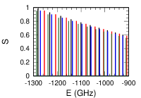
Figure 2: A plot of the uncorrelated energies of Ho $F_{T}=12$ $s$- and $d$-Rydberg series. The energy is relative to the $F_{c}=23/2$ threshold which is the highest hyperfine energy of the ground state. The $S\propto 1/\nu^{3}$. The range -1300 GHz to -900 GHz corresponds to $\nu=50.3$ to $\nu=60.5$. The purple line is the $s$-Rydberg series attached to the $F_{c}=23/2$ threshold. The others are the two $d$-series attached to the 23/2 threshold (purple), two series attached to the 21/2 threshold (blue), and one series attached to the 19/2 threshold (green). There are several places showing the near degeneracy of states attached to different thresholds which could lead to strong state mixing.

In Figs. 2 and 3 we show a simple stick drawing of where uncorrelated Rydberg states appear in the spectrum to give an idea of the complications possible. The plots are for $F_{T}=12$ which has 6 Rydberg series attached to the ground hyperfine states. The height of each stick is proportional to $1/\nu^{3}$ to indicate the oscillator strength available for each state. In calculating these states, the $s$-Rydberg series have quantum defects near 4.32 plus 0.01 shifts depending on the channel and the $d$-Rydberg series have quantum defects near 2.71 plus 0.01 shifts depending on the channel. For these plots, there are two $d$-Rydberg series attached to the $F_{c}=23/2$ and 21/2 threshold that are too close together to distinguish in the plots.

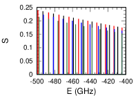
Figure 3: Same as Fig. 2 but for a smaller range. The range -500 GHz to -400 GHz corresponds to $\nu=81.1$ to $\nu=90.7$.

Although there are more Rydberg series for $F_{T}=11$, these plots already show quite complicated spectra. There are several places where states attached to different threshold are nearly degenerate. For example, near -971 GHz, two $d$-states attached to the $F_{c}=21/2$ threshold are nearly degenerate with the $s$-series attached to the $F_{c}=23/2$ threshold. As another example, there are 5 states in the 200 MHz range between -404.47 and -404.27 GHz: 2 $d$-states attached to the $F_{c}=23/2$ threshold, 2 $d$-states attached to the $F_{c}=21/2$ threshold and one $d$-state attached to the $F_{c}=19/2$ threshold.

Figure 4: A plot of the $d$-series photoabsorption cross section for $F_{T}=12$ using a linearly polarized photon with $M_{Ti}=1$. The taller series of peaks is one of the $d$-series attached to the $F_{c}=23/2$ state and the medium series is one of the series attached to the $F_{c}=21/2$ state. The series attached to the $F_{c}=19/2$ threshold is $\sim 100$ times smaller than the strong series.

Figure 5: Same as Fig. 4.

The rest of the results we present include channel interactions caused by the hyperfine splitting of the Ho⁺.

Figures 4 and 5 give an idea of what the photoabsorption cross section would look like for the transition from the initial state of Ref. Hostetter et al. (2015) to the $F_{T}=12$ series if only the $d$-series were present. For linearly polarized light in the $z$-direction, the cross section is 0 if $M_{T}=0$ so we chose $M_{T}=1$. We chose a linewidth of 50 MHz so the spectra would not be a series of delta functions. We use the frame transformation for the dipole matrix element as described in Sec. II.6.1 and the K-matrix as described in Sec. II.2 but with no corrections of the jj-coupled K-matrix. We randomly assigned quantum defects to the LS-channels, the coupling of Fig. 1b), in the range seen by the experiment.Hostetter et al. (2015) The values we chose for $\mu(SL)$ were: 2.85, 2.83, 2.81, 2.79 for $S=5/2$, $L=8-5$ and 2.77, 2.75, 2.73 for $S=3/2$, $L=8-6$.

One of the interesting features is that most of the states have little oscillator strength. There are actually 5 Rydberg series with $F_{T}=12$ and $\ell=2$ as discussed above, but only 2 of the series are clearly visible in Fig. 4. The strongest series is one attached to the $F_{c}=23/2$ threshold and the next strongest is one attached to the $F_{c}=21/2$ threshold. None of the other 3 series has substantial oscillator strength. The small oscillator strength leads to a much simpler spectra compared to the actual energy levels. However, it must be remembered that those states are still present and that external fields or Rydberg-Rydberg interactions could cause strong mixing between these nearly degenerate states.

V.2 Zeeman Shift, Ho

The effect of a weak magnetic field on the Rydberg series is deceptively complicated due to the high density of states that can interact through the magnetic field. For example, our simple calculation gives 15 $d$-Rydberg levels in the 4 GHz region from $-489$ to $-485$ GHz with total angular momentum $F_{T}\geq 10$. However, if the experiment can restrict the states to high angular momentum, then the situation can be favorable for isolating states. For example, if the Ho initial $F_{Ti}=12$ is in the $M_{Ti}=12$ state and then excited to the Rydberg states with circularly polarized light then there are only two states with $F_{T}=13$ close in energy: $-486.659$ and $-487.275$ GHz with the first having more than 100 times the oscillator strength of the second. These states can only mix with the $F_{T}=14,M_{T}=13$ state at $-487.483$ GHz. Thus, if the $-486.659$ GHz state is excited, the closest states are over 600 MHz away and will not strongly mix. The closest $F_{T}=12$ states are $\simeq 210$ MHz away. Thus, even an alignment mismatch that allows some $M_{T}=12$ character will not have a large mixing with other states unless the Zeeman shifts are above $\sim 20$ MHz in this example.

To understand how the energies shift with magnetic field, we can treat the case where the magnetic field is in the $z$-direction. In this case, the Zeeman shifts are given by $\Delta E(M_{T})=\mu BM_{T}$ where we can use the Eqs. (22,24) to obtain an expression for the $\mu$:

$$\mu=\frac{\langle\Phi_{i}||\mu_{B}(\ell^{(1)}+L_{c}^{(1)}+g_{s}[S_{c}^{(1)}+s^{(1)}])]-\mu_{I}I^{(1)}||\Phi_{i}\rangle}{\sqrt{(2F_{T}+1)(F_{T}+1)F_{T}}}$$ (45)

where we have used an identity for the 3-j symbol when $F_{T}=F_{T}^{\prime}$ and $q=0$.

For the two $F_{T}=13$ states, the $-486.659$ GHz state has $\mu\simeq 0.85\mu_{B}$ and the $-487.275$ GHz has $0.92\mu_{B}$. The coupling between them is $\sim 0.01\mu_{B}$. The $F_{T}=14$ state at $-487.483$ GHz has $0.93\mu_{B}$. The $F_{T}=12$ states have $1.02\mu_{B}$, $0.92\mu_{B}$, and $0.84\mu_{B}$ in order of increasing energy. Thus, all of the states have a $\mu\sim\mu_{B}$ with a coupling roughly two orders of magnitude smaller.

V.3 Static Polarizability, Ho

The polarizability determines the quadratic energy shift of a state in an electric field, ${\cal E}$. The energy shift is $\Delta E=-(1/2)\alpha{\cal E}^{2}$. Comparing to Eq. (28), the polarizability can be written as $\alpha=-2H^{(2)}_{bb}|_{{\cal E}=1}$. Because the dipole matrix elements scale like $\nu^{2}$ and the energy differences scale like $1/\nu^{3}$, the polarizability scales as $\nu^{7}$. For states with total angular momentum greater than 1/2, there is both a scalar, $\alpha_{0}$, and tensor, $\alpha_{2}$, polarizability which captures the $M$-dependence of the energy shift. If the electric field is in the $z$-direction the change in energy is

$$\Delta E=-\frac{1}{2}\left(\alpha_{0}+\frac{3M^{2}-F(F+1)}{F(2F-1)}\alpha_{2}\right){\cal E}^{2}$$ (46)

where $F$ is the total angular momentum of the state and $M$ is its projection on the $z$-direction.

The quantum defects for the $p$-Rydberg series are not known very well but, from Refs. Manson (1969); Fano et al. (1976), they are expected to differ from the quantum defects of the $d$-series by approximately 1. Thus, the polarizability of the $d$-series can not be even qualitatively estimated with current knowledge because slight changes in their quantum defects could change the energy ordering of the states which would change the sign of the polarizability. However, the magnitude of the $d$-series polarizability should be relatively large due to the near degeneracy.

As an example, we computed the static polarizability for the $s$-Rydberg series with $F_{T}=12$. Reference Li et al. (2017b) computed the frequency dependent polarizability for the Ho ground level configuration. From the discussion above, we expect that this series does not have a rapidly varying quantum defect. In the calculation, the quantum defect was fixed at $\mu_{s}=4.34$. Since there is only one Rydberg series for this case, the energies are at $-1/(2\nu_{s}^{2})$ where $\nu_{s}=n-\mu_{s}$. For the $p$-series, we chose the LS-coupled quantum defects, the coupling in Fig. 1b), to be different values between 3.73 and 3.83. For each Rydberg state, $n$, we used all of the $p$-Rydberg states with $F_{T}=11,12,13$ that were between energies $-1/[2(\nu_{s}-6)^{2}]<E<-1/[2(\nu_{s}+6)^{2}]$ and checked that the results were converged by changing the energy range.

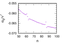
Figure 6: The scaled static scalar polarizability, $\alpha_{0}/\nu_{s}^{7}$, versus the principal quantum number, $n$, for the $s$-Rydberg series with $F_{T}=12$.

Figure 6 shows the static scalar polarizability scaled by its main dependence on $\nu$ and Fig. 7 shows the static tensor polarizability also scaled. The small magnitude of the tensor polarizability compared to the scalar indicates that the variation of energy with $M_{T}$ is not large. The small relative size of the tensor polarizability could be due to the fact that most of the polarizability arises from an $s$-Rydberg electron which would suppress the orientation dependence of the energy shift. Over the range shown, the scalar polarizability is negative which means the energy of a Rydberg state in this series will shift up in energy with an increasing electric field. The size of the scalar polarizability is relatively small because the $s$- and $p$-quantum defects differ by approximately 0.5. This means the $p$-states nearly evenly bracket each $s$-state which leads to the shift from each nearly canceling each other.

Because there are $p$-series attached to the $F_{c}=21/2$ and 19/2 thresholds, there are cases where $p$-states are nearly degenerate with an $s$-state. The effect of this can be seen near $n=62$ and 86. Both the scalar and tensor polarizabilities have a sharp variation near these cases. The variation is not as large as might be expected because the near degeneracy means the $p$-state wave function has a character that mostly consists of the wrong core state. Thus, the dipole matrix element is smaller than might be expected for the nearly degenerate state. An interesting case is at $n=62$ where the tensor polarizability changes sign. For most of the $n$, the energy shift becomes smaller as $M_{T}$ increases, but the energy shift increases with increasing $M_{T}$ at $n=62$.

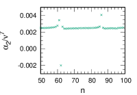
Figure 7: The scaled static tensor polarizability, $\alpha_{2}/\nu_{s}^{7}$, versus the principal quantum number, $n$, for the $s$-Rydberg series with $F_{T}=12$.

For the real Ho atom, the $n$ where the resonance condition occurs will probably be different from what was shown in this section. The energy where the degeneracy occurs depends on the actual values of the quantum defects. However, the number of regions where there is a sharp variation should be $\simeq 2$ because that depends on the threshold spacing which is well known.

VI Two atom example results

VI.1 $C_{5}$ coefficient, Ho

We implemented the equations for the $C_{5}$ coefficients, Eq. (40). As an example, we calculated all of these coefficients for the $F_{T}=13$ state at $-486.659$ GHz discussed in the Zeeman shift section. The states are labeled by the sum of the $z$-components of the total angular momentum $M_{T}=M_{T1}+M_{T2}$. The number of states at $M_{T}$ is ${\cal N}=2F_{T}-M_{T}+1$. The eigenstates are even or odd with respect to interchange of the atoms. There is one more even eigenstate than odd when ${\cal N}$ is odd, otherwise there are the same number of even and odd states.

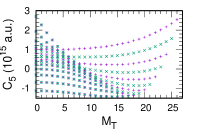
Figure 8: The eigenvalues of the $C_{5}$ coefficients as a function of the total $z$-component of the angular momenta, $M_{T}=M_{T1}+M_{T2}$. The even states (+) and odd states (X) are plotted. The $C_{5}$ are in atomic units and scaled by the factor $10^{15}$. To convert to GHz $\mu$m⁵, multiply by $2.73\times 10^{-15}$.

The results are plotted in Fig. 8. Because the $F_{T}=13$, the maximum $z$-component of angular momentum is 26. The states with negative $M_{T}$ are not plotted since the eigenvalues do not depend on the sign of $M_{T}$. The overall size of the $C_{5}$ should be $\sim\nu^{8}$ because there is a product of two $r^{2}$ matrix elements, each of which scales like $\nu^{4}$. Because this state is a mixture of Rydberg character with different thresholds, there is a rough value $\nu\sim 82$ for this state giving $C_{5}\sim 82^{8}\sim 2\times 10^{15}$. The $C_{5}$ is roughly this size. Converting to a frequency scale, the largest energy is $E\sim 7GHz/R^{5}$ with $R$ in $\mu$m which suggests this interaction will not be important in most applications.

There is an interesting pattern to the eigenvalues. For large $M_{T}$, the even and odd eigenvalues are quite distinct because the eigenvectors span all of the states so that even and odd states have non-zero amplitude for states with $M_{T1}\simeq M_{T2}$. As the $M_{T}$ becomes less than $\sim 15$, an increasing number of states have nearly the same eigenvalue for even and odd states. This is because these states are mostly localized to large values of the difference in the projections (i.e. large values of $|M_{T1}-M_{T2}|$). Since these states have small amplitude for $M_{T1}\simeq M_{T2}$, there is little amplitude to distinguish even from odd states. These states are like a double well potential with a large barrier.

VI.2 $C_{6}$ coefficient, Ho

As with the calculation of the polarizability, the $d$-Rydberg series will be difficult to predict due to the near degeneracy from the $p$-Rydberg series. So as with the polarizability, results are presented for the $s$-Rydberg series with $F_{T}=12$ which can only mix with the $p$-Rydberg series. As with the calculation of the $C_{5}$ coefficient, there are even and odd eigenstates with respect to interchange of atoms, with the number of states following the same pattern as for the $C_{5}$. The size of the $C_{6}$ coefficient is expected to scale with $\nu^{11}$ (four powers of dipole matrix element each scaling like $\nu^{2}$ divided by an energy difference which scales like $\nu^{-3}$).

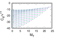
Figure 9: The eigenvalues of the scaled $C_{6}$ coefficients as a function of the total $z$-component of the angular momenta, $M_{T}=M_{T1}+M_{T2}$. The even states (+) and odd states (X) are plotted. The case plotted is $n=50$. To convert to GHz $\mu$m⁶, multiply by $1.44\times 10^{-19}$.

Figure 9 shows the $M_{T}$ dependence of the eigenvalues of the $C_{6}$ matrix scaled by the expected $\nu$-dependence. The state plotted is $n=50$ which is far from the cases that are sensitive to $n$. As with the $C_{5}$ eigenvalues, there is an interesting pattern to the even and odd eigenvalues. Unlike the $C_{5}$ case, the even and odd values are distinct except for the eigenvalue with smallest magnitude. All of the eigenvalues are negative which leads to an attractive potential between the atoms independent of the $M_{T}$. The size of the $C_{6}$ coefficients spans a wide range of values: over a factor of 6 from the smallest to largest in magnitude. The overall size of the van der Waals interaction for this series is not especially strong. At $n=50$, the smallest magnitude $C_{6}$ is approximately a factor of $\sim 20$ smaller than that for Rb $50d_{5/2}50d_{5/2}$ with $M_{T}=5$ while the largest magnitude Ho $C_{6}$ is a factor of $\sim 3$ times smaller.

It is difficult to show the dependence of the $C_{6}$ on $n$ for all of the possible $M_{T}$. In Fig. 10, the scaled $C_{6}$ for the four even states with largest $M_{T}$ are shown. As with the polarizability, there are two places ($n\sim 77$ and 95) where the $C_{6}$ varies rapidly with $n$. The values for $n=77$ are not shown because they are a factor of $\sim-20$ of the average value. For these states, only the $n=77$ leads to a positive $C_{6}$ which gives a repelling potential between the two atoms. The actual $C_{6}$ near these sensitive $n$ can not be predicted with the current state of knowledge of Ho. However, it is likely that there will be cases of strong $C_{6}$.

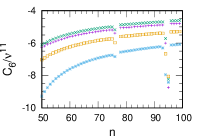
Figure 10: The eigenvalues of the scaled $C_{6}$ coefficients as a function of the principal quantum number $n$. The $M_{T}=24$ even states (+), $M_{T}=23$ even states (X), and the two $M_{T}=22$ even states (square and asterisk) are plotted. To convert to GHz $\mu$m⁶, multiply by $1.44\times 10^{-19}$.

VII Summary

We have derived the equations that can be used to treat the Rydberg states of atoms where the core state has sizable hyperfine splitting. This could be interesting for rare earth atoms where the ground state of the ion can have very large angular momentum as well as many hyperfine levels.

The theory is developed using the tools of multichannel quantum defect theory (MQDT). We have derived the equations for both single atom properties and two atom properties. For a single atom, we have given expressions for finding the energy levels, oscillator strengths, Zeeman mixing and shifts, and Stark mixing and shifts. For an atom pair, we have shown how to calculate the Rydberg-Rydberg interactions in general and have derived the specific cases for the $C_{5}$ and $C_{6}$ coefficients.

Although the treatment above should be accurate enough for many applications, the theory needs substantial input from measurements of the single atom properties. This might be a challenge for many atoms. Although the Rydberg states are not known well enough for any of the rare earths, we made estimates of parameters for Ho and used the estimates to demonstrate how to implement the equations for both single atom and two atom parameters. These results give a cartoon picture how the parameters might behave in a real atom.

VIII acknowledgment

This work was supported by the National Science Foundation under award No.1404419-PHY (FR) and award No.1707854-PHY (DWB and MS).

References

- Gallagher (1994) T.F. Gallagher, Rydberg atoms (Cambridge University Press, Cambridge, 1994).
- Lu et al. (2011) M. Lu, N. Q. Burdick, S. H. Youn, and B. L. Lev, “Strongly dipolar Bose-Einstein condensate of dysprosium,” Phys. Rev. Lett. 107, 190401 (2011).
- Lu et al. (2012) M. Lu, N. Q. Burdick, and B. L. Lev, “Quantum degenerate dipolar Fermi gas,” Phys. Rev. Lett. 108, 215301 (2012).
- Aikawa et al. (2012) K. Aikawa, A. Frisch, M. Mark, S. Baier, A. Rietzler, R. Grimm, and F. Ferlaino, “Bose-einstein condensation of Erbium,” Phys. Rev. Lett. 108, 210401 (2012).
- Frisch et al. (2014) A. Frisch, M. Mark, K. Aikawa, F. Ferlaino, J. L. Bohn, C. Makrides, A. Petrov, and S. Kotochigova, “Quantum chaos in ultracold collisions of gas-phase Erbium atoms,” Nature 507, 475 (2014).
- Schmitt et al. (2016) M. Schmitt, M. Wenzel, F. Böttcher, I. Ferrier-Barbut, and T. Pfau, “Self-bound droplets of a dilute magnetic quantum liquid,” Nature 539, 259 (2016).
- Saffman and Mølmer (2008) M. Saffman and K. Mølmer, “Scaling the neutral-atom Rydberg gate quantum computer by collective encoding in Holmium atoms,” Phys. Rev. A 78, 012336 (2008).
- Daley et al. (2008) A. J. Daley, M. M. Boyd, J. Ye, and P. Zoller, “Quantum computing with alkaline-earth-metal atoms,” Phys. Rev. Lett. 101, 170504 (2008).
- Shibata et al. (2009) K. Shibata, S. Kato, A. Yamaguchi, S. Uetake, and Y. Takahashi, “A scalable quantum computer with ultranarrow optical transition of ultracold neutral atoms in an optical lattice,” Appl. Phys. B 97, 753 (2009).
- Mukherjee et al. (2011) R. Mukherjee, J. Millen, R. Nath, M. P. A. Jones, and T. Pohl, “Many-body physics with alkaline-earth Rydberg lattices,” J. Phys. B 44, 184010 (2011).
- Topcu and Derevianko (2014) T. Topcu and A. Derevianko, “Divalent Rydberg atoms in optical lattices: Intensity landscape and magic trapping,” Phys. Rev. A 89, 023411 (2014).
- Topcu and Derevianko (2016) T. Topcu and A. Derevianko, “Possibility of triple magic trapping of clock and Rydberg states of divalent atoms in optical lattices,” J. Phys. B 49, 144004 (2016).
- Gil et al. (2014) L. I. R. Gil, R. Mukherjee, E. M. Bridge, M. P. A. Jones, and T. Pohl, “Spin squeezing in a Rydberg lattice clock,” Phys. Rev. Lett. 112, 103601 (2014).
- Khazali et al. (2016) M. Khazali, H. W. Lau, A. Humeniuk, and C. Simon, “Large energy superpositions via Rydberg dressing,” Phys. Rev. A 94, 023408 (2016).
- Aymar et al. (1996) Mireille Aymar, Chris H Greene, and Eliane Luc-Koenig, “Multichannel Rydberg spectroscopy of complex atoms,” Rev. Mod. Phys. 68, 1015 (1996).
- Vaillant et al. (2012) C.L. Vaillant, M.P.A. Jones, and R.M. Potvliege, “Long-range Rydberg - Rydberg interactions in calcium, strontium and ytterbium,” J. Phys. B 45, 135004 (2012).
- Vaillant et al. (2014) C. L. Vaillant, M. P. A. Jones, and R. M. Potvliege, “Multichannel quantum defect theory of strontium bound Rydberg states,” J. Phys. B 47, 155001 (2014), erratum: ibid 47, 199601 (2014).
- Rinneberg and Neukammer (1982) H. Rinneberg and J. Neukammer, “Hyperfine structure and configuration interaction of the 5d7d perturbing state of barium,” J. Phys. B 15, L825 (1982).
- Rinneberg and Neukammer (1983) H. Rinneberg and J. Neukammer, “Hyperfine structure and three-channel quantum-defect theory of rydberg states of ba,” Phys. Rev. A 27, 1779 (1983).
- Eliel and Hogervorst (1983) E. R. Eliel and W. Hogervorst, “Hyperfine structure in 6snd Rydberg configurations in barium,” J. Phys. B 16, 1881 (1983).
- Aymar (1984a) M. Aymar, “Multichannel-quantum-defect theory wave functions of Ba tested or improved by laser measurements,” J. Opt. Soc. Am. B 1, 239 (1984a).
- Beigang et al. (1983) R. Beigang, W. Makat, A. Timmermann, and P. J. West, “Hyperfine-induced mixing in high Rydberg states of ,” Phys. Rev. Lett. 51, 771 (1983).
- Nörtershäuser et al. (2000) W. Nörtershäuser, B. A. Bushaw, and K. Blaum, “Double-resonance measurements of isotope shifts and hyperfine structure in Gd I with hyperfine-state selection in an intermediate level,” Phys. Rev. A 62, 022506 (2000).
- Jin et al. (2011) W.-G. Jin, Hiroaki Ono, and T. Minowa, “Hyperfine structure and isotope shift in high-lying levels of Gd I,” J. Phys. Soc. Japan 80, 124301 (2011).
- Ray et al. (1988) D. Ray, B. Kundu, and P. K. Mukherjee, “Rydberg states and spin-forbidden transitions of the beryllium isoelectronic sequence,” J. Phys. B: At. Mol. Opt. Phys. 21, 3191 (1988).
- Yoshida et al. (2006) F. Yoshida, L. Matsuoka, R. Takashima, T. Nagata, Y. Azuma, S. Obara, F. Koike, and S. Hasegawa, “Analysis of rydberg states in the -shell photoionization of the Be atom,” Phys. Rev. A 73, 062709 (2006).
- Beigang and Schmidt (1981) R. Beigang and D. Schmidt, “Two-photon spectroscopy of 3snd 1d2 Rydberg states of magnesium I,” Phys. Lett. A 87, 21 (1981).
- Wehlitz et al. (2007) R. Wehlitz, D. Lukic, and P. N. Juranic, “Observation of a new 3s 3pnd double-excitation Rydberg series in ground-state magnesium,” J. Phys. B: At. Mol. Opt. Phys 40, 2385 (2007).
- Beigang et al. (1982) R. Beigang, K. Lücke, D. Schmidt, A. Timmermann, and P. J. West, “One-photon laser spectroscopy of Rydberg series from metastable levels in Calcium and Strontium,” Phys. Scr. 26, 183 (1982).
- Gentile et al. (1990) T. R. Gentile, B. J. Hughey, Daniel Kleppner, and T. W. Ducas, “Microwave spectroscopy of calcium Rydberg states,” Phys. Rev. A 42, 440 (1990).
- Cooke et al. (1978) W. E. Cooke, T. F. Gallagher, S. A. Edelstein, and R. M. Hill, “Doubly excited autoionizing Rydberg states of Sr,” Phys. Rev. Lett. 40, 178 (1978).
- Mauger et al. (2007) S. Mauger, J. Millen, and M. P. A. Jones, “Spectroscopy of strontium Rydberg states using electromagnetically induced transparency,” J. Phys. B: At. Mol. Opt. Phys 40, F319 (2007).
- Aymar (1984b) M. Aymar, “Rydberg series of alkaline-earth atoms Ca through Ba. the interplay of laser spectroscopy and multichannel quantum defect analysis,” Phys. Rep. 110, 163 (1984b).
- Sun and Lu (1988) J.-Q. Sun and K. T. Lu, “Hyperfine structure of extremely high Rydberg msns and msns series in odd alkaline-earth isotopes,” J. Phys. B: At. Mol. Opt. Phys. 21, 1957 (1988).
- Sun (1989) J.-Q. Sun, “Multichannel quantum defect theory of the hyperfine structure of high Rydberg states,” Phys. Rev. A 40, 7355 (1989).
- Sun et al. (1989) J.-Q. Sun, K.T. Lu, and R. Beigang, “Hyperfine structure of extremely high Rydberg msnd 1D2, 3D1, 3D2 and 3D3 series in odd alkaline-earth isotopes,” J. Phys. B 22, 2887 (1989).
- Wörner et al. (2003) H. Wörner, U. Hollenstein, and F. Merkt, “Multichannel quantum defect theory and high-resolution spectroscopy of the hyperfine structure of high Rydberg states of 83Kr,” Phys. Rev. A 68, 032510 (2003).
- Schäfer and Merkt (2006) M. Schäfer and F. Merkt, “Millimeter-wave spectroscopy and multichannel quantum-defect-theory analysis of high Rydberg states of krypton: The hyperfine structure of 83kr+,” Phys. Rev. A 74, 062506 (2006).
- Schäfer et al. (2010) M. Schäfer, M. Raunhardt, and F. Merkt, “Millimeter-wave spectroscopy and multichannel quantum-defect-theory analysis of high Rydberg states of xenon: The hyperfine structure of 129Xe+ and 131Xe+,” Phys. Rev. A 81, 032514 (2010).
- Xue et al. (1997) P. Xue, X. Y. Xu, W. Huang, C. B. Xu, R. C. Zhao, and X. P. Xie, “Observation of the highly excited states of Lanthanum,” AIP Conf. Proc. 388, 299 (1997).
- Sun et al. (2001) W. Sun, P. Xue, X. P. Xie, W. Huang, C. B. Xu, Z. P. Zhong, and X. Y. Xu, “Atomic triply excited double Rydberg states of lanthanum investigated by selective laser excitation,” Phys. Rev. A 64, 031402 (2001).
- Jayasekharan et al. (2000) T. Jayasekharan, M. A. N. Razvi, and G. L. Bhale, “Even-parity bound and autoionizing Rydberg series of the samarium atom,” J. Phys. B: At. Mol. Opt. Phys. 33, 3123 (2000).
- Wen-Jie et al. (2009) Q. Wen-Jie, D. Chang-Jian, X. Ying, and Z. Hong-Ying, “Experimental study of highly excited even-parity bound states of the Sm atom,” Chin. Phys. B 18, 3384 (2009).
- Zhao et al. (2011) Y.-H. Zhao, C.-J. Dai, and S.-W. Ye, “Study on even-parity highly excited states of the Sm atom,” J. Phys. B: At. Mol. Opt. Phys. 44, 195001 (2011).
- Shah et al. (2014) M.L. Shah, A.C. Sahoo, A.K. Pulhani, G.P. Gupta, B.M. Suri, and Vas Dev, “Investigations of high-lying even-parity energy levels of atomic samarium using simultaneous observation of two-color laser-induced fluorescence and photoionization signals,” Eur. Phys. J. D 68, 235 (2014).
- Nakhate et al. (2000) S. G. Nakhate, M. A. N. Razvi, J. P. Connerade, and S. A. Ahmad, “Investigation of Rydberg states of the europium atom using resonance ionization spectroscopy,” J. Phys. B: At. Mol. Opt. Phys. 33, 5191 (2000).
- Xie et al. (2011) J. Xie, C.-J. Dai, and M. Li, “Study of even-parity highly excited states of Eu I with a three-colour stepwise resonant excitation,” J. Phys. B: At. Mol. Opt. Phys. 44, 015002 (2011).
- Bhattacharyya et al. (2007) S. Bhattacharyya, M. A. N. Razvi, S. Cohen, and S. G. Nakhate, “Odd-parity autoionizing Rydberg series of europium below the threshold: Spectroscopy and multichannel quantum-defect-theory analysis,” Phys. Rev. A 76, 012502 (2007).
- Wang et al. (2012) X. Wang, L. Shen, and C.-J. Dai, “Interaction among different Rydberg series of the europium atom,” J. Phys. B: At. Mol. Opt. Phys. 45, 165001 (2012).
- Miyabe et al. (1998) M. Miyabe, M. Oba, and I. Wakaida, “Analysis of the even-parity Rydberg series of Gd I to determine its ionization potential and isotope shift,” J. Phys. B: At. Mol. Opt. Phys. 31, 4559 (1998).
- Ankush and Deo (2013) B. K. Ankush and M. N. Deo, “Experimental studies on electronic configuration mixing for the even-parity levels of Gd I using isotope shifts recorded in the visible region with FTS,” J. Spectros. 2013, 741020 (2013).
- Xu et al. (1992) X. Y. Xu, H. J. Zhou, W. Huang, and D. Y. Chen, “RIMS studies of high Rydberg and autoionizing states of the rare-earth element Dy,” Inst. Phys. Conf. Ser. 128, 71 (1992).
- Studer et al. (2016) D. Studer, P. Dyrauf, P. Naubereit, R. Heinke, and K. Wendt, “Resonance ionization spectroscopy in dysprosium,” Hyp. Inter. 238 (2016).
- Hostetter et al. (2015) J. Hostetter, J.D. Pritchard, J.E. Lawler, and M. Saffman, “Measurement of holmium Rydberg series through magneto-optical trap depletion spectroscopy,” Phys. Rev. A 91, 012507 (2015).
- Vidolova-Angelova et al. (1989) E. P. Vidolova-Angelova, D. A. Angelov, T. B. Krustev, and S. T. Mincheva, “Laser spectroscopy measurement of radiative lifetimes of highly excited thulium Rydberg states,” J. Opt. Soc. Am. B , 2295 (1989).
- Camus et al. (1980) P. Camus, A. Debarre, and C. Morillon, “Highly excited levels of neutral ytterbium. I. Two-photon and two-step spectroscopy of even spectra,” J. Phys. B: At. Mol. Opt. Phys. 13, 1073 (1980).
- Aymar et al. (1984) M. Aymar, R. J. Champeau, C. Delsart, and O. Robaux, “Three-step laser spectroscopy and multichannel quantum defect analysis of odd-parity Rydberg states of neutral ytterbium,” J. Phys. B: At. Mol. Opt. Phys 17, 3645 (1984).
- Ali et al. (1999) R. Ali, M. Yaseen, A. Nadeem, S. A. Bhatti, and M. A. Baig, “Two-colour three-photon excitation of the 6snf 1,3F3 and 6snp 1P1, 3P1,2 Rydberg levels of Yb I,” J. Phys. B: At. Mol. Opt. Phys 32, 953 (1999).
- Zinkstok et al. (2002) R. Zinkstok, E. J. van Duijn, S. Witte, and W. Hogervorst, “Hyperfine structure and isotope shift of transitions in Yb I using UV and deep-UV cw laser light and the angular distribution of fluorescence radiation,” J. Phys. B: At. Mol. Opt. Phys. 35, 2693 (2002).
- Ogawa and Kujirai (1999) Y. Ogawa and O. Kujirai, “Study of even-parity autoionization states of lutetium atom by atomic beam laser resonance ionization spectroscopy,” J. Phys. Soc. Jpn. 68, 428 (1999).
- Dai et al. (2003) Z. Dai, J. Zhankui, H. Xu, Z. Zhiguo, S. Svanberg, E. Biémont, P. H. Lefèbvre, and P. Quinet, “Time-resolved laser-induced fluorescence measurements of Rydberg states in Lu I and comparison with theory,” J. Phys. B: At. Mol. Opt. Phys 36, 479 (2003).
- Li et al. (2017a) R. Li, J. Lassen, Z. P. Zhong, F. D. Jia, M. Mostamand, X. K. Li, B. B. Reich, A. Teigelhöfer, and H. Yan, “Even-parity Rydberg and autoionizing states of lutetium by laser resonance-ionization spectroscopy,” Phys. Rev. A 95, 052501 (2017a).
- Worden et al. (1978) E. F. Worden, R. W. Solarz, J. A. Paisner, and J. G. Conway, “First ionization potentials of Lanthanides by laser spectroscopy,” J. Opt. Soc. Am. 68, 52 (1978).
- Lawler et al. (2004) J.E. Lawler, C. Sneden, and J.J. Cowan, “Improved atomic data for Ho II and new holmium abundances for the sun and three metal-poor stars,” Astr. J. 604, 850 (2004).
- Edmonds (1974) A.R. Edmonds, Angular Momentum in Quantum Mechanics, 2nd Edition (Princeton University Press, Princeton, New Jersey, 1974).
- Bhattii et al. (1981) S.A. Bhattii, C.L. Cromer, and W.E. Cooke, “Analysis of the Rydberg character of the D2 state of barium,” Phys. Rev. A 24, 161 (1981).
- Cowan (1981) R.D. Cowan, The Theory of Atomic Structure and Spectra (University of California Press, Berkeley and Los Angeles, California, 1981).
- Kramida et al. (2015) A. Kramida, Yu. Ralchenko, J. Reader, and and NIST ASD Team, NIST Atomic Spectra Database (ver. 5.3), [Online]. Available: http://physics.nist.gov/asd [2017, October 6]. National Institute of Standards and Technology, Gaithersburg, MD. (2015).
- Rose (1958) M.E. Rose, “The electrostatic interaction of two arbitrary charge distributions,” J. Math. Phys. 37, 215 (1958).
- Fontana (1961) P.R. Fontana, “Theory of long-range interatomic forces. I. Dispersion energies between unexcited atoms,” Phys. Rev. 123, 1865 (1961).
- Dalgarno and Davison (1966) A. Dalgarno and W.D. Davison, “The calculation of van der Waals interactions,” Adv. At. Mol. Phys. 2, 1 (1966).
- Weber et al. (2017) S. Weber, C. Tresp, H. Menke, A. Urvoy, O. Firstenberg, H.P. Büchler, and S. Hofferberth, “Calculation of Rydberg interaction potentials,” J. Phys. B 50, 133001 (2017).
- Walker and Saffman (2008) Thad G. Walker and M. Saffman, “Consequences of Zeeman degeneracy for the van der Waals blockade between Rydberg atoms,” Phys. Rev. A 77, 032723 (2008).
- Manson (1969) S.T. Manson, “Dependence of the phase shift on energy and atomic number for electron scattering by atomic fields,” Phys. Rev. 182, 97 (1969).
- Fano et al. (1976) U. Fano, C.E. Theodosiou, and J.L. Dehmer, “Electron-optical properties of atomic fields,” Rev. Mod. Phys. 48, 49 (1976).
- Li et al. (2017b) Hui Li, Jean-Francois Wyart, Olivier Dulieu, and Maxence Lepers, “Anisotropic optical trapping as a manifestation of the complex electronic structure of ultracold lanthanide atoms: The example of holmium,” Phys. Rev. A 95, 062508 (2017b).