Computer assisted proof of the existence of the Lorenz attractor in the Shimizu-Morioka system

Maciej J. Capiński 111This work was partially supported by the Polish National Science Centre grants 2015/19/B/ST1/01454, 2016/21/B/ST1/02453 and by the Faculty of Applied Mathematics AGH UST statutory tasks 11.11.420.004 within subsidy of Ministry of Science and Higher Education. Faculty of Applied Mathematics, AGH University of Science and Technology, Mickiewicza 30, 30-059 Kraków, Poland maciej.capinski@agh.edu.pl    Dmitry Turaev 222This work was supported by the RSF grant 14-41-00044. The support of EPSRC is gratefully acknowledged. Imperial College, London SW7 2AZ, United Kingdom,
and Lobachevsky University of Nizhni Novgorod, pr. Gagarina 23, 603950, Nizhny Novgorod, Russia
d.turaev@imperial.ac.uk
   Piotr Zgliczyński 333This work was supported by the Polish National Science Centre grant 2015/19/B/ST1/01454 Institute of Computer Science, Faculty of Mathematics and Computer Science, Jagiellonian University, ul. S. Łojasiewicza 6, 30-348 Kraków, Poland umzglicz@cyf-kr.edu.pl, piotr.zgliczynski@ii.uj.edu.pl
Abstract

We prove that the Shimizu-Morioka system has a Lorenz attractor for an open set of parameter values. For the proof we employ a criterion proposed by Shilnikov, which allows to conclude the existence of the attractor by examination of the behaviour of only one orbit. The needed properties of the orbit are established by using computer assisted numerics. Our result is also applied to the study of local bifurcations of triply degenerate periodic points of three-dimensional maps. It provides a formal proof of the birth of discrete Lorenz attractors at various global bifurcations.

1 Introduction and main results

In this paper we provide a solution to a long-standing open problem. We prove, by employing rigorous numerics, that Shimizu-Morioka system has a Lorenz attractor for an open set of parameter values. The fact itself is well-known, see [ASh1, ASh2, SST]; however its rigorous proof was missing which created a formal obstacle to some further developments in the mathematical theory of homoclinic bifurcations (see remarks in Section 1.4). Here, we report a computer assisted proof which closes this problem. Note that the use of computer assistance is sufficiently mild here, since we employ a Shilnikov criterion that allows us to conclude the existence of the Lorenz attractor in our system by examination of the behavior of only a single orbit of the system (see Sections 1.3 and 1.5).

The Shimizu-Morioka system

{x˙=y,y˙=(1z)xλy,z˙=αz+x2,cases˙𝑥𝑦˙𝑦1𝑧𝑥𝜆𝑦˙𝑧𝛼𝑧superscript𝑥2\left\{\begin{array}[]{l}\dot{x}=y,\\ \dot{y}=(1-z)x-\lambda y,\\ \dot{z}=-\alpha z+x^{2},\end{array}\right. (1)

where (x,y,z)𝑥𝑦𝑧(x,y,z) are coordinates in 3superscript3\mathbb{R}^{3} and α>0𝛼0\alpha>0, λ>0𝜆0\lambda>0 are parameters, was introduced by T.Shimizu and N.Morioka in [SM] and extensively studied numerically by A. Shilnikov in [ASh1, ASh2]. One of the main findings was that there is a large open region in the (α,λ)𝛼𝜆(\alpha,\lambda)-plane where this system has a strange attractor very similar to the classical attractor of the Lorenz model (5), see Fig. 1. This is more than just the similarity in shape: as one can infer from the pictures numerically obtained in [ASh1], the Poincaré map on a two-dimensional cross-section is hyperbolic (very strongly contracting in one direction and expanding in the other direction), so the attractor in the Shimizu-Morioka system can be described by the Afraimovich-Bykov-Shilnikov geometric Lorenz model [ABS77, ABS82], i.e., it is a Lorenz attractor.

Refer to caption
Refer to caption
Figure 1: Two kinds of Lorenz attractors in the Shimizu-Morioka system: standard (for α=0.45𝛼0.45\alpha=0.45, λ=0.9𝜆0.9\lambda=0.9) on the left, and with a lacuna (for α=0.5𝛼0.5\alpha=0.5, λ=0.85𝜆0.85\lambda=0.85) on the right.

We will describe the geometric Lorenz model and give the corresponding definition of the Lorenz attractors in a moment. However, we first want to stress that Shimizu-Morioka model is special (and maybe more important than the classical Lorenz model). The reason is that system (1) is a truncated normal form for certain codimension-3 bifurcations of equilibria and periodic orbits [SST, PST]. Because Lorenz or Lorenz-like attractors persist at small perturbations, our result on the existence of the Lorenz attractor in the normal form system (1) implies that Lorenz-like attractors exist for any small perturbation of (1). This proves the emergence of the Lorenz attractor (or its discrete analogue) in the corresponding class of codimension-3 bifurcations. In particular, in this paper, using Theorem 3, we prove the existence of discrete Lorenz attractors in a class of three-dimensional polynomial maps (3D Hénon maps, see Theorem 4).

1.1 Pseudohyperbolicity

In order to talk about Lorenz attractors, we need a proper definition of them. Classical definitions go back to the Guckenheimer-Williams [G76, GW, W79, Ro] and Afraimovich-Bykov-Shilnikov [ABS77, ABS82] geometric models; modern generalisations can be found in [MPP]. Here we use the Afraimovich-Bykov-Shilnikov model for Lorenz attractors, which we describe using the notion of pseudo-hyperbolicity introduced in [TSH98, TSH07]. A system (a smooth flow or a diffeomorphism) in nsuperscript𝑛\mathbb{R}^{n} is called pseudo-hyperbolic in a strictly forward-invariant domain 𝒟n𝒟superscript𝑛{\cal D}\subseteq\mathbb{R}^{n} if:

1) there are directions in which the dynamical system (a flow or a diffeomorphism) is strongly contracting (“strongly” means that any possible contraction in transverse directions is always strictly weaker);

2) transverse to the contracting directions the system is volume-expanding (i.e. the volume is stretched exponentially).

In precise terms, condition 1 reads as follows. For each point of 𝒟𝒟\cal D, we assume that there exists a pair of transversal subspaces N1subscript𝑁1N_{1} and N2subscript𝑁2N_{2} (with dim(N2)=k1𝑑𝑖𝑚subscript𝑁2𝑘1dim(N_{2})=k\geq 1 and dim(N1)=nk𝑑𝑖𝑚subscript𝑁1𝑛𝑘dim(N_{1})=n-k), continuously depending on the point, such that the families of these subspaces are invariant with respect to the derivative DXt𝐷subscript𝑋𝑡DX_{t} of the time-t𝑡t map Xtsubscript𝑋𝑡X_{t} of the system, i.e., DXtN1(x)=N1(Xt(x))𝐷subscript𝑋𝑡subscript𝑁1𝑥subscript𝑁1subscript𝑋𝑡𝑥DX_{t}N_{1}(x)=N_{1}(X_{t}(x)) and DXtN2(x)=N2(Xt(x))𝐷subscript𝑋𝑡subscript𝑁2𝑥subscript𝑁2subscript𝑋𝑡𝑥DX_{t}N_{2}(x)=N_{2}(X_{t}(x)) for all t0𝑡0t\geq 0 (in the case of a diffeomorphism, t𝑡t runs all positive integer values). We also assume that there exist constants C>0𝐶0C>0, α>0𝛼0\alpha>0 and β>0𝛽0\beta>0 such that for each x𝒟𝑥𝒟x\in\cal D and all t0𝑡0t\geq 0

DXt(x)|N2Ceαt\|DX_{t}(x)|_{N_{2}}\|\leq Ce^{-\alpha t} (2)

and

DXt(x)|N2(DXt(x)|N1)1Ceβt.\|DX_{t}(x)|_{N_{2}}\|\cdot\|(DX_{t}(x)|_{N_{1}})^{-1}\|\leq Ce^{-\beta t}. (3)

The volume-expansion condition 2 reads as follows: there exist constants C>0𝐶0C>0 and σ>0𝜎0\sigma>0 such that for each x𝒟𝑥𝒟x\in\cal D and all t0𝑡0t\geq 0

det(DXt(x)|N1)Ceσt.𝑑𝑒𝑡evaluated-at𝐷subscript𝑋𝑡𝑥subscript𝑁1𝐶superscript𝑒𝜎𝑡det(DX_{t}(x)|_{N_{1}})\geq Ce^{\sigma t}. (4)

Inequality (3) (the so-called cone condition) ensures that the invariant families of subspaces N1subscript𝑁1N_{1} and N2subscript𝑁2N_{2} continuously persist for all C1superscript𝐶1C^{1}-small perturbations of the system, so the pseudohyperbolic structure is a robust property of the system. Inequality (4) guarantees that for every orbit in 𝒟𝒟\cal D its maximal Lyapunov exponent is positive. Therefore, the existence of the pseudohyperbolic structure in a bounded domain 𝒟𝒟\cal D ensures chaotic dynamics in 𝒟𝒟\cal D, which cannot be destroyed by small smooth perturbations.

Conditions (2),(3) imply also the existence of a strong-stable invariant foliation 𝒩sssuperscript𝒩𝑠𝑠{\cal N}^{ss} in 𝒟𝒟\cal D, whose field of tangents is the family N2subscript𝑁2N_{2}. For every two points in the same leaf of 𝒩sssuperscript𝒩𝑠𝑠{\cal N}^{ss} the distance between their forward orbits tends to zero exponentially, i.e., the forward dynamics of all points in the same leaf are the same.

1.2 Lorenz attractor

The Lorenz attractor of the Afraimovich-Bykov-Shilnikov model is the attractor of a pseudohyperbolic system of differential equations with dim(N1)=2𝑑𝑖𝑚subscript𝑁12dim(N_{1})=2. Specifically, consider a system X𝑋X of differential equations with a saddle equilibrium state O𝑂O. Assume that O𝑂O has a one-dimensional unstable manifold Wu(O)superscript𝑊𝑢𝑂W^{u}(O) and an (n1)𝑛1(n-1)-dimensional stable manifold Ws(O)superscript𝑊𝑠𝑂W^{s}(O), i.e., if λ1,,λnsubscript𝜆1subscript𝜆𝑛\lambda_{1},\dots,\lambda_{n} are the eigenvalues of the linearized system at O𝑂O, then λ1>0subscript𝜆10\lambda_{1}>0 and Reλj<0𝑅𝑒subscript𝜆𝑗0Re\lambda_{j}<0 for j2𝑗2j\geq 2. Assume that

λ2>Reλj for j3formulae-sequencesubscript𝜆2𝑅𝑒subscript𝜆𝑗 for 𝑗3\lambda_{2}>Re\lambda_{j}\quad\mbox{ for }j\geq 3

and

λ1+λ2>0.subscript𝜆1subscript𝜆20\lambda_{1}+\lambda_{2}>0.

This means that the pseudohyperbolicity conditions (2), (3) and (4) are fulfilled at the point O𝑂O, with N1subscript𝑁1N_{1} being the two-dimensional eigenspace corresponding to the eigenvalues λ1subscript𝜆1\lambda_{1} and λ2subscript𝜆2\lambda_{2} and N2subscript𝑁2N_{2} being the eigenspace corresponding to the rest of eigenvalues. We assume that the pseudohyperbolicity property also holds in a sufficiently large, bounded neighborhood 𝒟𝒟\cal D of O𝑂O. We assume that 𝒟𝒟\cal D is strictly forward-invariant, i.e., there exists T>0𝑇0T>0 such that the image of the closure of 𝒟𝒟\cal D by the time-T𝑇T map lies strictly inside 𝒟𝒟\cal D.

Moreover, we assume that in 𝒟𝒟\cal D there exists an (n1)𝑛1(n-1)-dimensional cross-section ΠΠ\Pi to the flow, such that for every point in 𝒟𝒟\cal D its forward orbit either tends to O𝑂O (i.e., it lies in Ws(O)superscript𝑊𝑠𝑂W^{s}(O)) or hits ΠΠ\Pi at some moment of time. We assume that ΠΠ\Pi is divided by a smooth (n2)𝑛2(n-2)-dimensional surface Π0subscriptΠ0\Pi_{0} into 2 halves, Π+subscriptΠ\Pi_{+} and ΠsubscriptΠ\Pi_{-}, such that the orbits starting in Π+subscriptΠ\Pi_{+} and ΠsubscriptΠ\Pi_{-} return to ΠΠ\Pi again, while the orbits starting in Π0subscriptΠ0\Pi_{0} tend to O𝑂O as t+𝑡t\to+\infty, i.e., Π0Ws(O)ΠsubscriptΠ0superscript𝑊𝑠𝑂Π\Pi_{0}\subset W^{s}(O)\cap\Pi. Thus, the orbits of X𝑋X define the Poincaré map T:Π+ΠΠ:𝑇subscriptΠsubscriptΠΠT:\Pi_{+}\cup\Pi_{-}\to\Pi.

This map is smooth outside the discontinuity surface Π0subscriptΠ0\Pi_{0}. The orbits starting close to Π0subscriptΠ0\Pi_{0} pass near O𝑂O, so the return time tends to infinity as the initial point M𝑀M tends to Π0subscriptΠ0\Pi_{0}; note that TM𝑇𝑀TM tends to one of the two points, M+subscript𝑀M_{+} and Msubscript𝑀M_{-}, where Wu(O)superscript𝑊𝑢𝑂W^{u}(O) intersects ΠΠ\Pi. The unstable manifold Wu(O)superscript𝑊𝑢𝑂W^{u}(O) is one-dimensional, so Wu(O)\O\superscript𝑊𝑢𝑂𝑂W^{u}(O)\backslash O consists of exactly two orbits, Γ+subscriptΓ\Gamma_{+} and ΓsubscriptΓ\Gamma_{-}, called separatrices, and the points M+subscript𝑀M_{+} and Msubscript𝑀M_{-} are the first points where the Γ+subscriptΓ\Gamma_{+} and ΓsubscriptΓ\Gamma_{-} intersect ΠΠ\Pi. We take the convention that limMΠ0T(M)subscript𝑀subscriptΠ0𝑇𝑀\lim_{M\to\Pi_{0}}T(M) equals to M+subscript𝑀M_{+} if the initial point M𝑀M approaches Π0subscriptΠ0\Pi_{0} from Π+subscriptΠ\Pi_{+} and Msubscript𝑀M_{-} if M𝑀M approaches Π0subscriptΠ0\Pi_{0} from ΠsubscriptΠ\Pi_{-}.

The invariant foliation 𝒩sssuperscript𝒩𝑠𝑠{\cal N}^{ss} of the system X𝑋X also corresponds to a codimension-1 strong-stable invariant foliation 𝒩Πsssubscriptsuperscript𝒩𝑠𝑠Π{\cal N}^{ss}_{\Pi} for the map T𝑇T: the leaves of 𝒩Πsssubscriptsuperscript𝒩𝑠𝑠Π{\cal N}^{ss}_{\Pi} are obtained as intersections with ΠΠ\Pi of the orbits of the leaves of 𝒩sssuperscript𝒩𝑠𝑠{\cal N}^{ss} by the flow. The foliation is contracting, i.e., the iterations by T𝑇T of any two points in the same leaf of 𝒩Πsssubscriptsuperscript𝒩𝑠𝑠Π{\cal N}^{ss}_{\Pi} converge exponentially to each other. However, the dynamics transverse to the strong-stable foliation are chaotic. The expansion of areas by the flow transverse to 𝒩sssuperscript𝒩𝑠𝑠{\cal N}^{ss} implies that the Poincaré map T𝑇T is uniformly expanding in the direction transverse to 𝒩Πsssubscriptsuperscript𝒩𝑠𝑠Π{\cal N}^{ss}_{\Pi}.

In other words, the pseudohyperbolicity of the flow in 𝒟𝒟\cal D implies that the Poincaré map T𝑇T is locally uniformly hyperbolic. However, one cannot directly apply the theory of uniform hyperbolicity to this map, as it has a singularity (at Π0subscriptΠ0\Pi_{0}). Nevertheless, the (singular) hyperbolicity of the Poincaré map T𝑇T makes a comprehensive analysis of the structure of the Lorenz attractor in the above described Afraimovich-Bykov-Shilnikov model possible, as it was done in [ABS82]. The results of these papers can be summarized as follows [OT17]:

Theorem 1.

[ABS82] Under conditions above, the set of non-wandering orbits of the system in 𝒟𝒟\cal D consists of a uniquely defined, two-dimensional closed invariant set 𝒜𝒟𝒜𝒟{\cal A}\subset{\cal D} (which is called the Lorenz attractor) and a (possibly empty) one-dimensional closed invariant set ΣΣ\Sigma (which may intersect 𝒜𝒜\cal A but is not a subset of 𝒜𝒜\cal A) such that
(1) the separatrices Γ+subscriptΓ\Gamma_{+} and ΓsubscriptΓ\Gamma_{-} and the saddle O𝑂O lie in 𝒜𝒜\cal A;
(2) 𝒜𝒜\cal A is transitive, and saddle periodic orbits are dense in 𝒜𝒜\cal A;
(3) 𝒜𝒜\cal A is the limit of a nested sequence of hyperbolic, transitive, compact invariant sets each of which is equivalent to a suspension over a finite Markov chain with positive topological entropy;
(4) 𝒜𝒜\cal A is structurally unstable: arbitrarily small smooth perturbations of the system lead to the creation of homoclinic loops to O𝑂O and to the subsequent birth and/or disappearance of saddle periodic orbits within 𝒜𝒜\cal A;
(5) when Σ=Σ\Sigma=\emptyset, the set 𝒜𝒜\cal A is the maximal attractor in 𝒟𝒟\cal D;
(6) when the set ΣΣ\Sigma is non-empty, it is a hyperbolic set equivalent to a suspension over a finite Markov chain (it may have zero entropy, e.g. be a single saddle periodic orbit);
(7) every forward orbit in 𝒟𝒟\cal D tends to 𝒜Σ𝒜Σ{\cal A}\cup\Sigma as t+𝑡t\to+\infty;
(8) when ΣΣ\Sigma\neq\emptyset, the maximal attractor in 𝒟𝒟\cal D is cl(Wu(Σ))=𝒜Wu(Σ)𝑐𝑙superscript𝑊𝑢Σ𝒜superscript𝑊𝑢Σcl(W^{u}(\Sigma))={\cal A}\cup W^{u}(\Sigma);
(9) A𝐴A attracts all orbits from its neighbourhood when 𝒜Σ=𝒜Σ{\cal A}\cap\Sigma=\emptyset.

In [ABS82] the pseudohyperbolicity conditions were expressed in a different (equivalent) form, as explicitly verifiable conditions that ensure the hyperbolicity of the Poincaré map T𝑇T. Similar hyperbolicity conditions were checked for the classical Lorenz model

x˙=10(xy),y˙=x(28z)y,z˙=83z+xyformulae-sequence˙𝑥10𝑥𝑦formulae-sequence˙𝑦𝑥28𝑧𝑦˙𝑧83𝑧𝑥𝑦\dot{x}=-10(x-y),\qquad\dot{y}=x(28-z)-y,\qquad\dot{z}=-\frac{8}{3}z+xy (5)

by W.Tucker, with the use of rigorous numerics. In this way, in [WT1, WT2], a computer assisted proof of the existence of the Lorenz attractor in system (5) was done.

1.3 Shilnikov criterion

In our approach to the proof of the existence of the Lorenz attractor in the Shimizu-Morioka system we also rely on the computer assistance, however we need much less computations. We use a criterion proposed by Shilnikov in [ShC, p. 240-241] that allows to show the existence of the Lorenz attractor by examination of the behavior of only one orbit (a separatrix) of the system of differential equations, instead of the direct check of the hyperbolicity of the Poincaré map T𝑇T which would require a high precision computation of a huge number of orbits.

In [ShC, p. 240-241], several criteria for the birth of the Lorenz attractor were proposed. We use the following one. Consider a system X𝑋X of differential equations in nsuperscript𝑛\mathbb{R}^{n}, which have a saddle equilibrium state O𝑂O with one-dimensional unstable manifold. Namely, let λ1,,λnsubscript𝜆1subscript𝜆𝑛\lambda_{1},\dots,\lambda_{n} are the eigenvalues of the linearized system at O𝑂O. We assume that

λ1> 0>λ2>Reλj for j3.formulae-sequencesubscript𝜆1 0subscript𝜆2𝑅𝑒subscript𝜆𝑗 for 𝑗3\lambda_{1}>\;0\;>\lambda_{2}>Re\lambda_{j}\quad\mbox{ for }j\geq 3.

Let the system be symmetric with respect to a certain involution \cal R and that O𝑂O is a symmetric equilibrium, i.e., O=O𝑂𝑂{\cal R}O=O. The eigenvectors e1subscript𝑒1e_{1} and e2subscript𝑒2e_{2} corresponding to the eigenvalues λ1subscript𝜆1\lambda_{1} and λ2subscript𝜆2\lambda_{2} must be \cal R-invariant. We assume that e1=e1subscript𝑒1subscript𝑒1{\cal R}e_{1}=-e_{1} and e2=e2subscript𝑒2subscript𝑒2{\cal R}e_{2}=e_{2}. This, in particular, implies that the two unstable separatrices Γ+subscriptΓ\Gamma_{+} and ΓsubscriptΓ\Gamma_{-}, which are tangent at O𝑂O to e1subscript𝑒1e_{1}, are symmetric to each other, Γ+=ΓsubscriptΓsubscriptΓ\Gamma_{+}={\cal R}\Gamma_{-}.

Let the system satisfy the following 3 conditions:

1. Assume that both separatrices Γ+subscriptΓ\Gamma_{+} and ΓsubscriptΓ\Gamma_{-} return to O as t+𝑡t\to+\infty and are tangent to the vector e2subscript𝑒2e_{2} when entering O𝑂O (it follows from the symmetry that they form a “homoclinic butterfly”, i.e., they enter O𝑂O from the same direction).

2. Assume that the so-called saddle value σ=λ1+λ2𝜎subscript𝜆1subscript𝜆2\sigma=\lambda_{1}+\lambda_{2} is zero.

3. Assume that the so-called separatrix value A𝐴A satisfies the condition

0<|A|<2.0𝐴20<|A|<2. (6)

The definition of the separatrix value for our case is given in Section 1.5, see (15). One can describe |A|𝐴|A| as the maximal extent, to which infinitesimal two-dimensional areas can be expanded by the system along the homoclinic loop (the sign of A𝐴A determines whether the orientation of the areas for which this maximal expansion is achieved is changed during the propagation along the loop); more about the definition of A𝐴A can be seen in [Rob1, Rob2, book].

According to [ShC, p. 240-241], bifurcations of systems satisfying the above described conditions lead to the birth of a Lorenz attractor. To make this statement precise, we note that conditions 1 and 2 describe a codimension-2 bifurcation in the class of \cal R-symmetric systems. Suppose the system is embedded into a two-parameter family of systems Xμ,εsubscript𝑋𝜇𝜀X_{\mu,\varepsilon} such that by changing the parameters μ𝜇\mu and ε𝜀\varepsilon we can independently vary the saddle value σ𝜎\sigma near zero and split the homoclinic loop Γ+subscriptΓ\Gamma_{+} (by the symmetry, the homoclinic loop ΓsubscriptΓ\Gamma_{-} will be split as well). Then we have

Theorem 2.

[ShC, p. 240-241] If condition (6) holds at the bifurcation moment (when the system Xμ,εsubscript𝑋𝜇𝜀X_{\mu,\varepsilon} has a homoclinic butterfly with a zero saddle value), then there exists an open region in the plane of parameters μ,ε𝜇𝜀\mu,\varepsilon, for which system Xμ,εsubscript𝑋𝜇𝜀X_{\mu,\varepsilon} has a Lorenz attractor of the Afraimovich-Bykov-Shilnikov model.

A proof of this result was given by Robinson in [Rob1, Rob2] under certain additional assumptions on the eigenvalues λ𝜆\lambda; in full generality this theorem was proven in [OT17].

We show in Theorems 5 and 6 that Shimizu-Morioka system (1) satisfies conditions 1-3 for some value of parameters (α,λ)𝛼𝜆(\alpha,\lambda) and that the homoclinic loops can be split and the saddle value can be varied independently when α𝛼\alpha and λ𝜆\lambda vary. This, as explained, implies our main result:

Theorem 3.

There exists an open set in the plane of parameters (α,λ)𝛼𝜆(\alpha,\lambda) for which the Shimizu-Morioka system has a Lorenz attractor.

1.4 Discrete Lorenz attractor in local and global bifurcations.

The main theorem can be applied to the study of local bifurcations of triply degenerate periodic points of three-dimensional maps. For example, consider a 3D Hénon-like map (x,y,z)(x¯,y¯,z¯)maps-to𝑥𝑦𝑧¯𝑥¯𝑦¯𝑧(x,y,z)\mapsto(\bar{x},\bar{y},\bar{z})

x¯=y,y¯=z,z¯=M1+Bx+M2yz2,formulae-sequence¯𝑥𝑦formulae-sequence¯𝑦𝑧¯𝑧subscript𝑀1𝐵𝑥subscript𝑀2𝑦superscript𝑧2\bar{x}=y,\qquad\bar{y}=z,\qquad\bar{z}=M_{1}+Bx+M_{2}y-z^{2}, (7)

where M1subscript𝑀1M_{1}, M2subscript𝑀2M_{2} and B𝐵B are parameters and (x,y,z)3𝑥𝑦𝑧superscript3(x,y,z)\in\mathbb{R}^{3}. Pictures numerically obtained in [GOST5] show that this map has a strange attractor which looks very similar to the Lorenz attractor, even though this is a discrete dynamical system and not a system of differential equations. The explanation to this fact (the emergence of a discrete analogue of a Lorenz attractor) can be obtained based on the following observation.

At M1=1/4subscript𝑀114M_{1}=-1/4, M2=1subscript𝑀21M_{2}=1, B=1𝐵1B=1 this map has a fixed point at x=y=z=1/2𝑥𝑦𝑧12x=y=z=1/2, and this point has all three multipliers (the eigenvalues of the linearization matrix at this point) on the unit circle: (1,1,1)111(-1,-1,1). This is a codimension-3 bifurcation and, as shown in [GOST5], the flow normal form for this bifurcation in this map is given by the Shimizu-Morioka system. More precisely, at (M1,M2,B)subscript𝑀1subscript𝑀2𝐵(M_{1},M_{2},B) close to (1/4,1,1)1411(-1/4,1,1) and (B+M11)2+4M1>0superscript𝐵subscript𝑀1124subscript𝑀10(B+M_{1}-1)^{2}+4M_{1}>0 we can shift the coordinate origin to the fixed point x=y=z=x=(B+M21+(B+M21)2+4M1)/2𝑥𝑦𝑧superscript𝑥𝐵subscript𝑀21superscript𝐵subscript𝑀2124subscript𝑀12x=y=z=x^{*}=(B+M_{2}-1+\sqrt{(B+M_{2}-1)^{2}+4M_{1}})/2. Then the map will take the form

x¯=y,y¯=z,z¯=Bx+M2y2xzz2.formulae-sequence¯𝑥𝑦formulae-sequence¯𝑦𝑧¯𝑧𝐵𝑥subscript𝑀2𝑦2superscript𝑥𝑧superscript𝑧2\bar{x}=y,\qquad\bar{y}=z,\qquad\bar{z}=Bx+M_{2}y-2x^{*}z-z^{2}. (8)

Introduce small parameters ε1=1Bsubscript𝜀11𝐵\varepsilon_{1}=1-B, ε2=1M2subscript𝜀21subscript𝑀2\varepsilon_{2}=1-M_{2}, ε3=2x1subscript𝜀32superscript𝑥1\varepsilon_{3}=2x^{*}-1. It was shown in [GOST5] that in the region ε1>0subscript𝜀10\varepsilon_{1}>0, ε1+ε3>ε2subscript𝜀1subscript𝜀3subscript𝜀2\varepsilon_{1}+\varepsilon_{3}>\varepsilon_{2}, the second iteration of (8) near the origin is O(s2)𝑂superscript𝑠2O(s^{2})-close, in appropriately chosen rescaled coordinates, to the time-s𝑠s shift by the flow of a system, which is O(s)𝑂𝑠O(s)-close to the Shimizu-Morioka system (1) with α=(ε1+ε2+ε3)/(4s)𝛼subscript𝜀1subscript𝜀2subscript𝜀34𝑠\alpha=(\varepsilon_{1}+\varepsilon_{2}+\varepsilon_{3})/(4s), λ=(ε1ε3)/(2s)𝜆subscript𝜀1subscript𝜀32𝑠\lambda=(\varepsilon_{1}-\varepsilon_{3})/(2s), s=(ε1ε2+ε3)/2𝑠subscript𝜀1subscript𝜀2subscript𝜀32s=\sqrt{(\varepsilon_{1}-\varepsilon_{2}+\varepsilon_{3})/2}. This means that if we make N𝑁N iterations of map (8), such that N𝑁N is even and of order s1superscript𝑠1s^{-1}, the result will be O(s)𝑂𝑠O(s)-close to the time-1 map of the Shimizu-Morioka system.

In other words, the N𝑁N-th iteration of map (8) is the time-1 map for a certain small, time-periodic perturbation of the Shimizu-Morioka system:

{x˙=y+f1(x,y,z,t),y˙=(1z)xλy+f2(x,y,z,t),z˙=αz+x2+f3(x,y,z,t),cases˙𝑥𝑦subscript𝑓1𝑥𝑦𝑧𝑡˙𝑦1𝑧𝑥𝜆𝑦subscript𝑓2𝑥𝑦𝑧𝑡˙𝑧𝛼𝑧superscript𝑥2subscript𝑓3𝑥𝑦𝑧𝑡\left\{\begin{array}[]{l}\dot{x}=y+f_{1}(x,y,z,t),\\ \dot{y}=(1-z)x-\lambda y+f_{2}(x,y,z,t),\\ \dot{z}=-\alpha z+x^{2}+f_{3}(x,y,z,t),\end{array}\right. (9)

where f1,2,3subscript𝑓123f_{1,2,3} are C1superscript𝐶1C^{1}-small functions, 1-periodic in time t𝑡t. According to [TSH07], the pseudohyperbolicity persists at small time-periodic perturbations. Therefore, as by Theorem 3 the Shimizu-Morioka system has a pseudohyperbolic attractor for an open set of (α,λ)𝛼𝜆(\alpha,\lambda) values, the same holds true for the map (8) for the corresponding set of values of ε1,2,3subscript𝜀123\varepsilon_{1,2,3}. This attractor is called a discrete Lorenz attractor because it shape is similar to the Lorenz attractor in the Shimizu-Morioka system. However, its structure is much more complicated than that of the Lorenz attractor described in section 1.2. In particular, the discrete Lorenz attractor may contain homoclinic tangencies [TSH07] and heterodimensional cycles involving saddle periodic orbits with different dimensions of the unstable manifold [LT18] (more discussions can be found in [GOT13]). This makes a complete description of the dynamics of the discrete Lorenz attractor impossible but, anyway, its pseudohyperbolicity allows to conclude that every orbit in this attractor is unstable and this property persists for all small perturbations.

Since the map (8) is obtained from (7) just by a change of coordinates, we have the following

Theorem 4.

There exists an open set in the space of parameters (M1,M2,B)subscript𝑀1subscript𝑀2𝐵(M_{1},M_{2},B) for which the 3D Hénon map (7) has a pseudohyperbolic discrete Lorenz attractor.

Note that the same conclusion holds for larger classes of three-dimensional maps. It was shown in [GOT13] that the normal form for the bifurcations of the zero fixed point of any map of the type

x¯¯𝑥\displaystyle\bar{x} =y,absent𝑦\displaystyle=y,
y¯¯𝑦\displaystyle\bar{y} =z,absent𝑧\displaystyle=z,
z¯¯𝑧\displaystyle\bar{z} =(1ε1)x+(1ε2)y(1+ε3)z+ay2+byz+cz2+O(x,y,z3),\displaystyle=(1-\varepsilon_{1})x+(1-\varepsilon_{2})y-(1+\varepsilon_{3})z+ay^{2}+byz+cz^{2}+O(\|x,y,z\|^{3}),

is the Shimizu-Morioka system, provided the condition

(ca)(ab+c)>0𝑐𝑎𝑎𝑏𝑐0(c-a)(a-b+c)>0 (10)

is fulfilled. Therefore, by the same arguments as for the map (8), Theorem 3 provides a formal justification for the claim of [GOT13] (see Lemma 3.1 there) about the existence of pseudohyperbolic attractors for an open set of parameters ε1,2,3subscript𝜀123\varepsilon_{1,2,3} in maps (1.4) whose coefficients satisfy condition (10).

Map (8) is particularly important for the theory of global bifurcations because it appears as a normal form for the first-return maps near many types of homoclinic tangencies and heteroclinic cycles with tangencies in three-dimensional and higher-dimensional maps [GGS]. Given a homoclinic or heteroclinic cycle, one can estimate its effective dimension — the maximal possible number of zero Lyapunov exponents that periodic orbits born at bifurcations of such cycle can have [T96]. Several different classes of maps with effectively 3-dimensional homoclinic or heteroclinic cycles were considered in [GMO, GST9, GI, GIT, GI17, O17]. It was shown in these papers that the corresponding bifurcations should produce pseudohyperbolic (discrete Lorenz) attractors. Namely, it was shown that a generic three-parameter unfolding of each of these bifurcations creates regions in the phase space where the first-return map is closely (as close as one wants) approximated, in appropriately chosen coordinates, by the 3D-Hénon map (8). Therefore, by the robustness of the pseudohyperbolicity property, the birth of the pseudohyperbolic Lorenz-like attractors at each of these bifurcations is established once the existence of a pseudohyperbolic attractor is shown in map (8).

As we mentioned, the first numerical evidence for the existence of such attractor in map (8) was obtained in [GOST5]. Theorem 4 makes it a rigorous result. Thus, now we have a full formal proof to the results of [GMO, GST9, GI, GIT, GI17, O17] about the emergence of pseudohyperbolic attractors at bifurcations of effectively 3-dimensional homoclinic and heteroclinic cycles, including the birth of infinitely many coexisting pseudohyperbolic attractors in some situations, see [GST9, GI].

1.5 Main results of the rigorous numerics

We establish Theorem 3 in the following steps. First, we find good bounds for the values of parameters (α,λ)𝛼𝜆(\alpha,\lambda) for which Shimizu-Morioka system (1) satisfies conditions 1 and 2 of Section 1.3 (the existence of a homoclinic butterfly with zero saddle value σ𝜎\sigma). It is easy to check that condition σ=0𝜎0\sigma=0 reads as

λ=1αα.𝜆1𝛼𝛼\lambda=\frac{1}{\alpha}-\alpha. (11)

We will study how the separatrices Γ±subscriptΓplus-or-minus\Gamma_{\pm} move as α𝛼\alpha varies while λ𝜆\lambda is given by (11); the moment a separatrix forms a homoclinic loop corresponds to the parameter values we are looking for.

It is convenient to scale time tt/α=T𝑡𝑡𝛼𝑇t\to t/\alpha=T and variables xx/α=X𝑥𝑥𝛼𝑋x\to x/\sqrt{\alpha}=X, yy/(αα)=Y𝑦𝑦𝛼𝛼𝑌y\to y/(\alpha\sqrt{\alpha})=Y. Then the system takes the form

X˙˙𝑋\displaystyle\dot{X} =Y,absent𝑌\displaystyle=Y,
Y˙˙𝑌\displaystyle\dot{Y} =(a+1)(1Z)XaY,absent𝑎11𝑍𝑋𝑎𝑌\displaystyle=\left(a+1\right)\left(1-Z\right)X-aY, (12)
Z˙˙𝑍\displaystyle\dot{Z} =Z+X2,absent𝑍superscript𝑋2\displaystyle=-Z+X^{2},

where

a=1α21=λ/α.𝑎1superscript𝛼21𝜆𝛼a=\frac{1}{\alpha^{2}}-1=\lambda/\alpha.

The eigenvalues of the linearization matrix at (0,0,0)000(0,0,0) are (1,1,(1+a))111𝑎(-1,1,-(1+a)) with corresponding eigenvectors given by (0,0,1)001(0,0,1), (1,1,0)110(1,1,0) and ((1+a)1,1,0)superscript1𝑎110(-(1+a)^{-1},1,0), respectively. We will investigate (12) for a1.72𝑎1.72a\approx 1.72, so the hyperbolic equilibrium state (0,0,0)000(0,0,0) has a one dimensional unstable manifold, and a two dimensional stable manifold. When the manifolds intersect, we have a solution that tends to zero both as t+𝑡t\to+\infty and t𝑡t\to-\infty, i.e., a homoclinic loop to the equilibrium state.

Theorem 5.

There exists a=a0[al,ar]𝑎subscript𝑎0subscript𝑎𝑙subscript𝑎𝑟a=a_{0}\in\left[a_{l},a_{r}\right], where

alsubscript𝑎𝑙\displaystyle a_{l} =1.724323291515411013,absent1.72432329151541superscript1013\displaystyle=1.72432329151541-10^{-13},
arsubscript𝑎𝑟\displaystyle a_{r} =1.72432329151541+1013,absent1.72432329151541superscript1013\displaystyle=1.72432329151541+10^{-13},

for which (12) has a homoclinic orbit X0(t),Y0(t),Z0(t)subscript𝑋0𝑡subscript𝑌0𝑡subscript𝑍0𝑡X_{0}\left(t\right),Y_{0}\left(t\right),Z_{0}\left(t\right) to the equilibrium state (0,0,0)000(0,0,0). As a𝑎a changes between alsubscript𝑎𝑙a_{l} and arsubscript𝑎𝑟a_{r}, the loop splits. Taking

ξ=1104,c=3.5,T=26,formulae-sequence𝜉1superscript104formulae-sequence𝑐3.5𝑇26\xi=1-10^{-4},\qquad c=3.5,\qquad T=26,

we have the bound:

|X0(T+t)|,|Y0(T+t)|,|Z0(T+t)|ceξt(X0(T),Y0(T),Z0(T)),subscript𝑋0𝑇𝑡subscript𝑌0𝑇𝑡subscript𝑍0𝑇𝑡𝑐superscript𝑒𝜉𝑡normsubscript𝑋0𝑇subscript𝑌0𝑇subscript𝑍0𝑇\left|X_{0}\left(T+t\right)\right|,\left|Y_{0}\left(T+t\right)\right|,\left|Z_{0}\left(T+t\right)\right|\leq ce^{-\xi t}\left\|\left(X_{0}\left(T\right),Y_{0}\left(T\right),Z_{0}\left(T\right)\right)\right\|,

for t0𝑡0t\geq 0, and for t0𝑡0t\leq 0 we have:

|X0(t)|,|Y0(t)|,|Z0(t)|ceξ|t|(X0(0),Y0(0),Z0(0)).subscript𝑋0𝑡subscript𝑌0𝑡subscript𝑍0𝑡𝑐superscript𝑒𝜉𝑡normsubscript𝑋00subscript𝑌00subscript𝑍00\left|X_{0}\left(t\right)\right|,\left|Y_{0}\left(t\right)\right|,\left|Z_{0}\left(t\right)\right|\leq ce^{-\xi\left|t\right|}\left\|\left(X_{0}\left(0\right),Y_{0}\left(0\right),Z_{0}\left(0\right)\right)\right\|.

The proof of the above theorem is obtained with a computer assistance and is given in section 3.2. The mere existence of a homoclinic loop in system (12) can be obtained purely analytically [TT]. However, we need good estimates on a0subscript𝑎0a_{0} and the corresponding homoclinic solution, which the methods of [TT] do not provide. Crucially, these estimates are used in the next theorem where the separatrix value A𝐴A is estimated.

The separatrix value can be defined as follows (cf. [Rob1, Rob2, TT]). Let a system of three differential equations have a homoclinic solution (X0(t),Y0(t),Z0(t))subscript𝑋0𝑡subscript𝑌0𝑡subscript𝑍0𝑡(X_{0}(t),Y_{0}(t),Z_{0}(t)) to a hyperbolic equilibrium state at zero, so (X0(t),Y0(t),Z0(t))0subscript𝑋0𝑡subscript𝑌0𝑡subscript𝑍0𝑡0(X_{0}(t),Y_{0}(t),Z_{0}(t))\to 0 as t±𝑡plus-or-minust\to\pm\infty. Let

ddt(xyz)=B(t)(xyz)𝑑𝑑𝑡𝑥𝑦𝑧𝐵𝑡𝑥𝑦𝑧\frac{d}{dt}\left(\begin{array}[]{c}x\\ y\\ z\end{array}\right)=B(t)\left(\begin{array}[]{c}x\\ y\\ z\end{array}\right) (13)

be the linearization of the system along the loop. In particular, in the case of system (12) we have

B=(010(a0+1)(1Z0(t))a0(a0+1)X0(t)2X0(t)01).𝐵010subscript𝑎011subscript𝑍0𝑡subscript𝑎0subscript𝑎01subscript𝑋0𝑡2subscript𝑋0𝑡01B=\left(\begin{array}[]{ccc}0&1&0\\ (a_{0}+1)(1-Z_{0}(t))&-a_{0}&-(a_{0}+1)X_{0}(t)\\ 2X_{0}(t)&0&-1\end{array}\right).

Let ξ1subscript𝜉1\xi_{1}, ξ2subscript𝜉2\xi_{2} be any two vectors and let η=ξ1×ξ2𝜂subscript𝜉1subscript𝜉2\eta=\xi_{1}\times\xi_{2} be their vector product. If the evolution of ξ1subscript𝜉1\xi_{1} and ξ2subscript𝜉2\xi_{2} is defined by (13), then the evolution of η𝜂\eta is governed by

dηdt=(Btr(B)I)η,𝑑𝜂𝑑𝑡superscript𝐵top𝑡𝑟𝐵𝐼𝜂\frac{d\eta}{dt}=-(B^{\top}-tr(B)I)\eta, (14)

where I𝐼I is the (3×3)33(3\times 3) identity matrix. This equation describes the evolution of infinitesimal two-dimensional areas near the homoclinic loop.

Since (X0(t),Y0(t),Z0(t))subscript𝑋0𝑡subscript𝑌0𝑡subscript𝑍0𝑡(X_{0}(t),Y_{0}(t),Z_{0}(t)) tends to zero exponentially, the asymptotic behavior of solutions of (14) as t±𝑡plus-or-minust\to\pm\infty is determined by the limit matrix

B^=(Btr(B)I)^𝐵superscriptsubscript𝐵top𝑡𝑟subscript𝐵𝐼\hat{B}=-(B_{\infty}^{\top}-tr(B_{\infty})I)

where B=limt±B(t)subscript𝐵subscript𝑡plus-or-minus𝐵𝑡B_{\infty}=\lim_{t\to\pm\infty}B(t), which is the linearization of the original system at the hyperbolic equilibrium at zero. If λ1>0>λ2>λ3subscript𝜆10subscript𝜆2subscript𝜆3\lambda_{1}>0>\lambda_{2}>\lambda_{3} are the eigenvalues of Bsubscript𝐵B_{\infty}, then the eigenvalues of B^^𝐵\hat{B} are

σ1=λ1+λ2,σ2=λ1+λ3,σ3=λ2+λ3.formulae-sequencesubscript𝜎1subscript𝜆1subscript𝜆2formulae-sequencesubscript𝜎2subscript𝜆1subscript𝜆3subscript𝜎3subscript𝜆2subscript𝜆3\sigma_{1}=\lambda_{1}+\lambda_{2},\qquad\sigma_{2}=\lambda_{1}+\lambda_{3},\qquad\sigma_{3}=\lambda_{2}+\lambda_{3}.

We are interested here in the case of zero saddle value, i.e., λ1+λ2=0subscript𝜆1subscript𝜆20\lambda_{1}+\lambda_{2}=0. Then the eigenvalues of B^^𝐵\hat{B} are 00, σ2<0subscript𝜎20\sigma_{2}<0 and σ3<0subscript𝜎30\sigma_{3}<0, so every solution of (14) tends, as t+𝑡t\to+\infty to a constant times the eigenvector of B^^𝐵\hat{B} that corresponds to the zero eigenvalue (this is the vector v0subscript𝑣0v_{0}, which is the vector product of the eigenvectors of Bsubscript𝐵B_{\infty} that correspond to the eigenvalues λ1subscript𝜆1\lambda_{1} and λ2subscript𝜆2\lambda_{2}). It also follows that only one solution of (14) tends to v0subscript𝑣0v_{0} in backward time, as t𝑡t\to-\infty. We take this particular solution η0(t)subscript𝜂0𝑡\eta_{0}(t) and denote

limt+η0(t)=Av0.subscript𝑡subscript𝜂0𝑡𝐴subscript𝑣0\lim_{t\to+\infty}\eta_{0}(t)=Av_{0}. (15)

The coefficient A𝐴A is the sought separatrix value. From the definition of A𝐴A one can see that

|A|=suplimt+η(t)η(t),𝐴supremumsubscript𝑡norm𝜂𝑡norm𝜂𝑡|A|=\sup\lim_{t\to+\infty}\frac{\|\eta(t)\|}{\|\eta(-t)\|},

where the supremum is taken over all the solutions of (14). Thus, A𝐴A determines the maximal expansion of infinitesimal areas along the homoclinic loop.

In the case of system (12) system (14) becomes

η(t)=((a0+1)(a0+1)(1Z0(t))2X0(t)1100(a0+1)X0(t)a0)η(t).superscript𝜂𝑡subscript𝑎01subscript𝑎011subscript𝑍0𝑡2subscript𝑋0𝑡1100subscript𝑎01subscript𝑋0𝑡subscript𝑎0𝜂𝑡\eta^{\prime}\left(t\right)=\left(\begin{array}[]{ccc}-\left(a_{0}+1\right)&-\left(a_{0}+1\right)\left(1-Z_{0}\left(t\right)\right)&-2X_{0}\left(t\right)\\ -1&-1&0\\ 0&\left(a_{0}+1\right)X_{0}\left(t\right)&-a_{0}\end{array}\right)\eta\left(t\right). (16)

This equation, in the limit t±𝑡plus-or-minust\rightarrow\pm\infty becomes

η(t)=B^η(t)=((a0+1)(a0+1)011000a0)η(t).superscript𝜂𝑡^𝐵𝜂𝑡subscript𝑎01subscript𝑎01011000subscript𝑎0𝜂𝑡\eta^{\prime}\left(t\right)=\hat{B}\eta\left(t\right)=\left(\begin{array}[]{ccc}-(a_{0}+1)&-(a_{0}+1)&0\\ -1&-1&0\\ 0&0&-a_{0}\end{array}\right)\eta\left(t\right). (17)

The eigenvalues are 0,(a+2),a0𝑎2𝑎0,-(a+2),-a with corresponding eigenvectors v0=(1,1,0)subscript𝑣0110v_{0}=(1,-1,0), v(a+2)=(1+a,1,0)subscript𝑣𝑎21𝑎10v_{-\left(a+2\right)}=(1+a,1,0) and va(0,0,1)subscript𝑣𝑎001v_{-a}(0,0,1), respectively.

Theorem 6.

There exists an orbit η(t)𝜂𝑡\eta\left(t\right) of (16), for which

limtη(t)subscript𝑡𝜂𝑡\displaystyle\lim_{t\rightarrow-\infty}\eta\left(t\right) \displaystyle\in [0.99984336210766,1.0001566378923]v0,0.999843362107661.0001566378923subscript𝑣0\displaystyle\left[0.99984336210766,1.0001566378923\right]v_{0},
limt+η(t)subscript𝑡𝜂𝑡\displaystyle\lim_{t\rightarrow+\infty}\eta\left(t\right) \displaystyle\in [0.62606812264791,0.62663392848044]v0,0.626068122647910.62663392848044subscript𝑣0\displaystyle[0.62606812264791,0.62663392848044]v_{0},

meaning that

limt+η(t)η(t)[0.62597007201516,0.6267320984754].subscript𝑡norm𝜂𝑡norm𝜂𝑡0.625970072015160.6267320984754\lim_{t\rightarrow+\infty}\frac{\left\|\eta\left(t\right)\right\|}{\left\|\eta\left(-t\right)\right\|}\in\left[0.62597007201516,0.6267320984754\right]. (18)

The proof of the above theorem is obtained with computer assistance and is given in Section 4.3. By definition (15) of the separatrix value, estimate (18) gives the following bounds for the separatrix value of the homoclinic loop in system (12):

A[0.62597007201516,0.6267320984754].𝐴0.625970072015160.6267320984754A\in\left[0.62597007201516,0.6267320984754\right].

Importantly 0<A<10𝐴10<A<1. So, by applying Shilnikov criterion we obtain our main result, Theorem 3, see section 1.3.

The plot of the homoclinic trajectory from Theorem 5 can be seen on the left plot in Figure 6 on page 6. The plot of the heteroclinic orbit from Theorem 6 is given in Figure 12 on page 12.

Remark 7.

The techniques we use for the proofs of Theorems 5 and 6 could also be used for the study of traveling waves and their stability in problems coming from PDEs on the line [wave1, wave2, wave3, wave4]. This is because proving their existence requires establishing the existence of heteroclinic/homoclinic connecting orbits. Investigating their stability requires studying additionally some linearized equations. We develop tools for such problems in Sections 3, 4.

2 Some notations

In the subsequent sections we present a methodology for establishing homoclinic orbits and for the computation of the separatrix value. First we introduce the following notations.

We will write Bk(R)subscript𝐵𝑘𝑅B_{k}(R) for ball in ksuperscript𝑘\mathbb{R}^{k} of radius R𝑅R, centered at zero. For a matrix A𝐴A we define the logarithmic norm of A𝐴A as (see [CZmelnikov] and literature cited there)

l(A)=limh0+I+AhIh.𝑙𝐴subscriptsuperscript0norm𝐼𝐴norm𝐼l\left(A\right)=\lim_{h\rightarrow 0^{+}}\frac{\left\|I+Ah\right\|-\left\|I\right\|}{h}.

We will also use the notation

m(A)𝑚𝐴\displaystyle m\left(A\right) =\displaystyle= {1A1detA0,0\firstchoice@falseotherwise,cases1superscriptnorm𝐴1𝐴00\firstchoice@falseotherwise,\displaystyle\left\{\begin{array}[]{l}\frac{1}{\left\|A\right\|^{-1}}\qquad\det A\neq 0,\\ 0\qquad\qquad\mathchoice{\hbox{{otherwise,}}}{\hbox{{\firstchoice@false otherwise,}}}{\hbox{{\firstchoice@false otherwise,}}}{\hbox{{\firstchoice@false otherwise,}}}\end{array}\right.
ml(A)subscript𝑚𝑙𝐴\displaystyle m_{l}\left(A\right) =\displaystyle= l(A).𝑙𝐴\displaystyle-l\left(-A\right).

The m(A)𝑚𝐴m(A) is a number with the property that Avm(A)v.norm𝐴𝑣𝑚𝐴norm𝑣\left\|Av\right\|\geq m\left(A\right)\left\|v\right\|. The ml(A)subscript𝑚𝑙𝐴m_{l}\left(A\right) can be interpreted as a ‘bound from below’ of the logarithmic norm.

Let u,s𝑢𝑠u,s\in\mathbb{N}. For a function f:u×su×s:𝑓superscript𝑢superscript𝑠superscript𝑢superscript𝑠f:\mathbb{R}^{u}\times\mathbb{R}^{s}\rightarrow\mathbb{R}^{u}\times\mathbb{R}^{s}, we will use the notations (x,y)u×s𝑥𝑦superscript𝑢superscript𝑠\left(x,y\right)\in\mathbb{R}^{u}\times\mathbb{R}^{s}, where xu𝑥superscript𝑢x\in\mathbb{R}^{u} and ys𝑦superscript𝑠y\in\mathbb{R}^{s}. The x𝑥x will play the role of an “unstable” coordinate and y𝑦y will be the “stable” coordinate, hence the choice of the notation u,s𝑢𝑠u,s. We will also write fxsubscript𝑓𝑥f_{x}, and fysubscript𝑓𝑦f_{y} for the projections of f𝑓f onto usuperscript𝑢\mathbb{R}^{u} and ssuperscript𝑠\mathbb{R}^{s}, respectively. For a set Du×s𝐷superscript𝑢superscript𝑠D\subset\mathbb{R}^{u}\times\mathbb{R}^{s} we define

[fxx(D)]delimited-[]subscript𝑓𝑥𝑥𝐷\displaystyle\left[\frac{\partial f_{x}}{\partial x}\left(D\right)\right] ::\displaystyle: ={A=(aij)u×u:ai,j[infpDfxixj(p),suppDfxixj(p)]},absentconditional-set𝐴subscript𝑎𝑖𝑗superscript𝑢𝑢subscript𝑎𝑖𝑗subscriptinfimum𝑝𝐷subscript𝑓subscript𝑥𝑖subscript𝑥𝑗𝑝subscriptsupremum𝑝𝐷subscript𝑓subscript𝑥𝑖subscript𝑥𝑗𝑝\displaystyle=\left\{A=\left(a_{ij}\right)\in\mathbb{R}^{u\times u}:a_{i,j}\in\left[\inf_{p\in D}\frac{\partial f_{x_{i}}}{\partial x_{j}}\left(p\right),\sup_{p\in D}\frac{\partial f_{x_{i}}}{\partial x_{j}}\left(p\right)\right]\right\},
[fxy(D)]delimited-[]subscript𝑓𝑥𝑦𝐷\displaystyle\left[\frac{\partial f_{x}}{\partial y}\left(D\right)\right] ::\displaystyle: ={A=(aij)u×s:ai,j[infpDfxiyj(p),suppDfxiyj(p)]}.absentconditional-set𝐴subscript𝑎𝑖𝑗superscript𝑢𝑠subscript𝑎𝑖𝑗subscriptinfimum𝑝𝐷subscript𝑓subscript𝑥𝑖subscript𝑦𝑗𝑝subscriptsupremum𝑝𝐷subscript𝑓subscript𝑥𝑖subscript𝑦𝑗𝑝\displaystyle=\left\{A=\left(a_{ij}\right)\in\mathbb{R}^{u\times s}:a_{i,j}\in\left[\inf_{p\in D}\frac{\partial f_{x_{i}}}{\partial y_{j}}\left(p\right),\sup_{p\in D}\frac{\partial f_{x_{i}}}{\partial y_{j}}\left(p\right)\right]\right\}.

We also define

m(fxx(D))𝑚subscript𝑓𝑥𝑥𝐷\displaystyle m\left(\frac{\partial f_{x}}{\partial x}\left(D\right)\right) :=assign\displaystyle:= infA[fxx(D)]m(A),subscriptinfimum𝐴delimited-[]subscript𝑓𝑥𝑥𝐷𝑚𝐴\displaystyle\inf_{A\in\left[\frac{\partial f_{x}}{\partial x}\left(D\right)\right]}m\left(A\right),
ml(fxx(D))subscript𝑚𝑙subscript𝑓𝑥𝑥𝐷\displaystyle m_{l}\left(\frac{\partial f_{x}}{\partial x}\left(D\right)\right) :=assign\displaystyle:= infA[fxx(D)]ml(A),subscriptinfimum𝐴delimited-[]subscript𝑓𝑥𝑥𝐷subscript𝑚𝑙𝐴\displaystyle\inf_{A\in\left[\frac{\partial f_{x}}{\partial x}\left(D\right)\right]}m_{l}\left(A\right),
fxy(D)normsubscript𝑓𝑥𝑦𝐷\displaystyle\left\|\frac{\partial f_{x}}{\partial y}\left(D\right)\right\| :=assign\displaystyle:= supA[fxy(D)]A.subscriptsupremum𝐴delimited-[]subscript𝑓𝑥𝑦𝐷norm𝐴\displaystyle\sup_{A\in\left[\frac{\partial f_{x}}{\partial y}\left(D\right)\right]}\left\|A\right\|.

We will use the notation int(D)int𝐷\mathrm{int}(D), D¯¯𝐷\overline{D} and D𝐷\partial D for the interior, closure and boundary of a set D𝐷D, respectively.

3 Establishing homoclinics

In this section we give an overview of the method for establishing the existence of homoclinic orbits to fixed points. The method is written for the case where we consider a parameter dependent ODE with the vector field f:3×3:𝑓superscript3superscript3f:\mathbb{R}^{3}\times\mathbb{R}\rightarrow\mathbb{R}^{3},

p=f(p,a).superscript𝑝𝑓𝑝𝑎p^{\prime}=f(p,a). (20)

and aA𝑎𝐴a\in A is a parameter, with A=[al,ar]𝐴subscript𝑎𝑙subscript𝑎𝑟A=[a_{l},a_{r}]\subset\mathbb{R}. We assume that for each aA𝑎𝐴a\in A (20) has a hyperbolic fixed point pasuperscriptsubscript𝑝𝑎p_{a}^{\ast}, with one dimensional unstable manifold and two dimensional stable manifolds. (If dimensions are the other way around we can change the sign of the vector field.)

Let Φt(p,a)subscriptΦ𝑡𝑝𝑎\Phi_{t}(p,a) be the flow induced by (20). Let B¯u(R)=[R,R]subscript¯𝐵𝑢𝑅𝑅𝑅\overline{B}_{u}\left(R\right)=\left[-R,R\right]\subset\mathbb{R}, B¯s(R)2subscript¯𝐵𝑠𝑅superscript2\overline{B}_{s}\left(R\right)\subset\mathbb{R}^{2} and let

D=B¯u(R)×B¯s(R)3,𝐷subscript¯𝐵𝑢𝑅subscript¯𝐵𝑠𝑅superscript3D=\overline{B}_{u}\left(R\right)\times\overline{B}_{s}\left(R\right)\subset\mathbb{R}^{3},

be a neighborhood of the smooth family of fixed points, meaning that we assume paintDsuperscriptsubscript𝑝𝑎int𝐷p_{a}^{\ast}\in\mathrm{int}D for any aA𝑎𝐴a\in A.

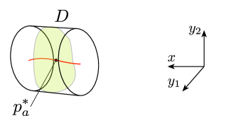
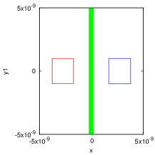
Refer to caption
Figure 2: The local unstable manifold Wausuperscriptsubscript𝑊𝑎𝑢W_{a}^{u} in red, and the local stable manifold Wassuperscriptsubscript𝑊𝑎𝑠W_{a}^{s} in green.

We denote by Wausuperscriptsubscript𝑊𝑎𝑢W_{a}^{u} the local unstable manifold of pasuperscriptsubscript𝑝𝑎p_{a}^{\ast} in D𝐷D and by Wassuperscriptsubscript𝑊𝑎𝑠W_{a}^{s} the local stable manifold of pasuperscriptsubscript𝑝𝑎p_{a}^{\ast} in D𝐷D, i.e.

Wausuperscriptsubscript𝑊𝑎𝑢\displaystyle W_{a}^{u} ={pD:Φt(p,a)D for t0 and limtΦt(p,a)=pa},absentconditional-set𝑝𝐷subscriptΦ𝑡𝑝𝑎𝐷 for 𝑡0 and subscript𝑡subscriptΦ𝑡𝑝𝑎superscriptsubscript𝑝𝑎\displaystyle=\left\{p\in D:\Phi_{t}\left(p,a\right)\in D\mathchoice{\hbox{{ for }}}{\hbox{{\firstchoice@false for }}}{\hbox{{\firstchoice@false for }}}{\hbox{{\firstchoice@false for }}}t\leq 0\mathchoice{\hbox{{ and }}}{\hbox{{\firstchoice@false and }}}{\hbox{{\firstchoice@false and }}}{\hbox{{\firstchoice@false and }}}\lim_{t\rightarrow-\infty}\Phi_{t}\left(p,a\right)=p_{a}^{\ast}\right\}, (21)
Wassuperscriptsubscript𝑊𝑎𝑠\displaystyle W_{a}^{s} ={pD:Φt(p,a)D for t0 and limt+Φt(p,a)=pa}.absentconditional-set𝑝𝐷subscriptΦ𝑡𝑝𝑎𝐷 for 𝑡0 and subscript𝑡subscriptΦ𝑡𝑝𝑎superscriptsubscript𝑝𝑎\displaystyle=\left\{p\in D:\Phi_{t}\left(p,a\right)\in D\mathchoice{\hbox{{ for }}}{\hbox{{\firstchoice@false for }}}{\hbox{{\firstchoice@false for }}}{\hbox{{\firstchoice@false for }}}t\geq 0\mathchoice{\hbox{{ and }}}{\hbox{{\firstchoice@false and }}}{\hbox{{\firstchoice@false and }}}{\hbox{{\firstchoice@false and }}}\lim_{t\rightarrow+\infty}\Phi_{t}\left(p,a\right)=p_{a}^{\ast}\right\}. (22)

We assume that Wausuperscriptsubscript𝑊𝑎𝑢W_{a}^{u} and Wassuperscriptsubscript𝑊𝑎𝑠W_{a}^{s} are graphs of C1superscript𝐶1C^{1} functions

wausuperscriptsubscript𝑤𝑎𝑢\displaystyle w_{a}^{u} :B¯u(R)B¯s(R),:absentsubscript¯𝐵𝑢𝑅subscript¯𝐵𝑠𝑅\displaystyle:\overline{B}_{u}\left(R\right)\rightarrow\overline{B}_{s}\left(R\right),
wassuperscriptsubscript𝑤𝑎𝑠\displaystyle w_{a}^{s} :B¯s(R)B¯u(R),:absentsubscript¯𝐵𝑠𝑅subscript¯𝐵𝑢𝑅\displaystyle:\overline{B}_{s}\left(R\right)\rightarrow\overline{B}_{u}\left(R\right),

meaning that (see Figure 2)

Wausuperscriptsubscript𝑊𝑎𝑢\displaystyle W_{a}^{u} ={(x,wau(x)):xB¯u(R)},absentconditional-set𝑥superscriptsubscript𝑤𝑎𝑢𝑥𝑥subscript¯𝐵𝑢𝑅\displaystyle=\left\{\left(x,w_{a}^{u}\left(x\right)\right):x\in\overline{B}_{u}\left(R\right)\right\},
Wassuperscriptsubscript𝑊𝑎𝑠\displaystyle W_{a}^{s} ={(was(y),y):yB¯s(R)}.absentconditional-setsuperscriptsubscript𝑤𝑎𝑠𝑦𝑦𝑦subscript¯𝐵𝑠𝑅\displaystyle=\left\{\left(w_{a}^{s}\left(y\right),y\right):y\in\overline{B}_{s}\left(R\right)\right\}. (23)
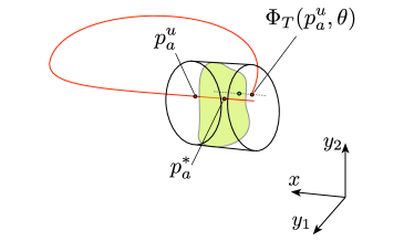
Refer to caption
Figure 3: We have the 111-dimensional unstable manifold of pasuperscriptsubscript𝑝𝑎p_{a}^{\ast} in red, and the 222-dimensional local stable manifold Wassuperscriptsubscript𝑊𝑎𝑠W_{a}^{s} in D𝐷D in green. The h(a)𝑎h\left(a\right) is the signed distance along the x𝑥x coordinate between Wassuperscriptsubscript𝑊𝑎𝑠W_{a}^{s} and ΦT(pau,a)subscriptΦ𝑇superscriptsubscript𝑝𝑎𝑢𝑎\Phi_{T}\left(p_{a}^{u},a\right); this is the distance along the dotted line on the plot.

Let

pau:=(R,wau(R))3.assignsuperscriptsubscript𝑝𝑎𝑢𝑅superscriptsubscript𝑤𝑎𝑢𝑅superscript3p_{a}^{u}:=\left(R,w_{a}^{u}\left(R\right)\right)\in\mathbb{R}^{3}. (24)

Consider T>0𝑇0T>0 and assume that for all aA𝑎𝐴a\in A, ΦT(pau,a)DsubscriptΦ𝑇superscriptsubscript𝑝𝑎𝑢𝑎𝐷\Phi_{T}\left(p_{a}^{u},a\right)\in D. Let us define

h:A,:𝐴h:A\rightarrow\mathbb{R},

as

h(a)=πxΦT(pau,a)was(πyΦT(pau,a)).𝑎subscript𝜋𝑥subscriptΦ𝑇superscriptsubscript𝑝𝑎𝑢𝑎superscriptsubscript𝑤𝑎𝑠subscript𝜋𝑦subscriptΦ𝑇superscriptsubscript𝑝𝑎𝑢𝑎h\left(a\right)=\pi_{x}\Phi_{T}\left(p_{a}^{u},a\right)-w_{a}^{s}(\pi_{y}\Phi_{T}\left(p_{a}^{u},a\right)). (25)

We now state a natural result, that h(a)=0𝑎0h\left(a\right)=0 implies an intersection of the stable and unstable manifolds of pasuperscriptsubscript𝑝𝑎p_{a}^{\ast}. (See Figure 3.)

Theorem 8.

[CW]If

h(al)<0andh(ar)>0formulae-sequencesubscript𝑎𝑙0andsubscript𝑎𝑟0h(a_{l})<0\qquad\mathchoice{\hbox{{and}}}{\hbox{{\firstchoice@false and}}}{\hbox{{\firstchoice@false and}}}{\hbox{{\firstchoice@false and}}}\qquad h(a_{r})>0 (26)

then there exists a ψA𝜓𝐴\psi\in A for which we have a homoclinic orbit to pψsuperscriptsubscript𝑝𝜓p_{\psi}^{\ast}.

3.1 Computer assisted bounds for unstable manifolds of fixed points of ODEs

In order to apply Theorem 8, we need to be able to establish bounds for hh defined in (25). Using a rigorous, interval arithmetic based integrator111in our application we use the CAPD package: http://capd.ii.uj.edu.pl/, it is possible to obtain rigorous enclosures for ΦTsubscriptΦ𝑇\Phi_{T}. In this section we discuss how to obtain bounds on parameterizations was,wausuperscriptsubscript𝑤𝑎𝑠superscriptsubscript𝑤𝑎𝑢w_{a}^{s},w_{a}^{u} of stable and unstable manifolds of fixed points. For simplicity, we will skip the parameter a𝑎a and consider an ODE

p=f(p).superscript𝑝𝑓𝑝p^{\prime}=f(p). (27)

When combined with Theorem 8, we can apply below results for (20) with fixed a.𝑎a.

Let Du×s𝐷superscript𝑢superscript𝑠D\subset\mathbb{R}^{u}\times\mathbb{R}^{s},

D=B¯u(R)×B¯s(R).𝐷subscript¯𝐵𝑢𝑅subscript¯𝐵𝑠𝑅D=\overline{B}_{u}\left(R\right)\times\overline{B}_{s}\left(R\right).

In this section we do not need to assume that u=1𝑢1u=1 and d=2.𝑑2d=2. The result works for arbitrary dimensions.

We define

μ𝜇\displaystyle\overrightarrow{\mu} =\displaystyle= supzD{l(fyy(z))+1Lfyx(z)},subscriptsupremum𝑧𝐷𝑙subscript𝑓𝑦𝑦𝑧1𝐿normsubscript𝑓𝑦𝑥𝑧\displaystyle\sup_{z\in D}\left\{l\left(\frac{\partial f_{y}}{\partial y}(z)\right)+\frac{1}{L}\left\|\frac{\partial f_{y}}{\partial x}(z)\right\|\right\}, (28)
ξ𝜉\displaystyle\overrightarrow{\xi} =\displaystyle= ml(fxx(D))Lfxy(D).subscript𝑚𝑙subscript𝑓𝑥𝑥𝐷𝐿normsubscript𝑓𝑥𝑦𝐷\displaystyle m_{l}\left(\frac{\partial f_{x}}{\partial x}(D)\right)-L\left\|\frac{\partial f_{x}}{\partial y}(D)\right\|. (29)
Definition 9.

We say that the vector field f𝑓f satisfies rate conditions if

μ<0<ξ,𝜇0𝜉\overrightarrow{\mu}<0<\overrightarrow{\xi}, (30)
Definition 10.

We say that D=B¯u(R)×B¯s(R)𝐷subscript¯𝐵𝑢𝑅subscript¯𝐵𝑠𝑅D=\overline{B}_{u}\left(R\right)\times\overline{B}_{s}\left(R\right) is an isolating block for (27) if

  1. 1.

    For any qB¯u(R)×B¯s(R)𝑞subscript¯𝐵𝑢𝑅subscript¯𝐵𝑠𝑅q\in\partial\overline{B}_{u}\left(R\right)\times\overline{B}_{s}\left(R\right),

    (πxf(q)|πxq)>0.conditionalsubscript𝜋𝑥𝑓𝑞subscript𝜋𝑥𝑞0\left(\pi_{x}f(q)|\pi_{x}q\right)>0.
  2. 2.

    For any qB¯u(R)×B¯s(R)𝑞subscript¯𝐵𝑢𝑅subscript¯𝐵𝑠𝑅q\in\overline{B}_{u}\left(R\right)\times\partial\overline{B}_{s}\left(R\right),

    (πyf(q)|πyq)<0.conditionalsubscript𝜋𝑦𝑓𝑞subscript𝜋𝑦𝑞0\left(\pi_{y}f(q)|\pi_{y}q\right)<0.
Definition 11.

We define the unstable set in D𝐷D as

Wu={z: Φt(z)D for all t<0}.superscript𝑊𝑢conditional-set𝑧 subscriptΦ𝑡𝑧𝐷 for all 𝑡0W^{u}=\{z:\mathchoice{\hbox{{ }}}{\hbox{{\firstchoice@false }}}{\hbox{{\firstchoice@false }}}{\hbox{{\firstchoice@false }}}\Phi_{t}(z)\in D\mathchoice{\hbox{{ for all }}}{\hbox{{\firstchoice@false for all }}}{\hbox{{\firstchoice@false for all }}}{\hbox{{\firstchoice@false for all }}}t<0\}.

Below theorem is a simplified (adapted to fixed points) version of the results from [CZmelnikov, Theorem 30]. The paper [CZmelnikov] is in the setting of normally hyperbolic invariant manifolds, hence the Theorem 30 from that paper is more involved than below result.

Theorem 12.

[CZmelnikov, Theorem 30] Let k1𝑘1k\geq 1. Assume that f𝑓f is C1superscript𝐶1C^{1} and satisfies the rate conditions. Assume also that D=B¯u(R)×B¯s(R)𝐷subscript¯𝐵𝑢𝑅subscript¯𝐵𝑠𝑅D=\overline{B}_{u}\left(R\right)\times\overline{B}_{s}\left(R\right) is an isolating block for f𝑓f. Then the set Wusuperscript𝑊𝑢W^{u} is a manifold, which is a graph over B¯u(R)subscript¯𝐵𝑢𝑅\overline{B}_{u}\left(R\right). To be more precise, there exists a C1superscript𝐶1C^{1} function

wu:B¯u(R)B¯s(R),:superscript𝑤𝑢subscript¯𝐵𝑢𝑅subscript¯𝐵𝑠𝑅w^{u}:\overline{B}_{u}(R)\rightarrow\overline{B}_{s}(R),

such that

Wu={(x,wu(x)):xB¯u(R)}.superscript𝑊𝑢conditional-set𝑥superscript𝑤𝑢𝑥𝑥subscript¯𝐵𝑢𝑅W^{u}=\left\{\left(x,w^{u}(x)\right):x\in\overline{B}_{u}(R)\right\}. (31)

Moreover, wusuperscript𝑤𝑢w^{u} is Lipschitz with constant L𝐿L.

Proof.

The proof is given in Appendix 6.1. It is a modification of the argument from [CZmelnikov]. The main difference is that the results from [CZmelnikov] are for the setting in which in addition to the hyperbolic coordinates x,y𝑥𝑦x,y we have a centre coordinate. Due to this the Lipschitz bound from Theorem 12 is sharper compared with [CZmelnikov]. In the proof we focus on this issue. ∎

We will now discuss the contraction rate along the stable manifold Wusuperscript𝑊𝑢W^{u} from Theorem 12. First we shall need an auxiliary result. Consider a flow Φt(z)subscriptΦ𝑡𝑧\Phi_{t}\left(z\right), for Φ:×u×su×s:Φsuperscript𝑢superscript𝑠superscript𝑢superscript𝑠\Phi:\mathbb{R\times R}^{u}\times\mathbb{R}^{s}\rightarrow\mathbb{R}^{u}\times\mathbb{R}^{s},

Φt(x,y)=(πxΦt(x,y),πyΦt(x,y)),subscriptΦ𝑡𝑥𝑦subscript𝜋𝑥subscriptΦ𝑡𝑥𝑦subscript𝜋𝑦subscriptΦ𝑡𝑥𝑦\Phi_{t}\left(x,y\right)=\left(\pi_{x}\Phi_{t}\left(x,y\right),\pi_{y}\Phi_{t}\left(x,y\right)\right),

and define the following constants

μ(h)𝜇\displaystyle\mu\left(h\right) =\displaystyle= supzD{πyΦy(h,z)+1LπyΦx(h,z)},subscriptsupremum𝑧𝐷normsubscript𝜋𝑦Φ𝑦𝑧1𝐿normsubscript𝜋𝑦Φ𝑥𝑧\displaystyle\sup_{z\in D}\left\{\left\|\frac{\partial\pi_{y}\Phi}{\partial y}\left(h,z\right)\right\|+\frac{1}{L}\left\|\frac{\partial\pi_{y}\Phi}{\partial x}\left(h,z\right)\right\|\right\}, (32)
ξ(h)𝜉\displaystyle\xi\left(h\right) =\displaystyle= m[πxΦx(h,D)]LsupzDπxΦy(h,z).𝑚delimited-[]subscript𝜋𝑥Φ𝑥𝐷𝐿subscriptsupremum𝑧𝐷normsubscript𝜋𝑥Φ𝑦𝑧\displaystyle m\left[\frac{\partial\pi_{x}\Phi}{\partial x}(h,D)\right]-L\sup_{z\in D}\left\|\frac{\partial\pi_{x}\Phi}{\partial y}\left(h,z\right)\right\|. (33)
Theorem 13.

[CZmelnikov, Theorem 31]Let ξ𝜉\overrightarrow{\xi} and μ𝜇\overrightarrow{\mu} be the constants defined in (28) and (29). If ΦtsubscriptΦ𝑡\Phi_{t} is the flow induced by (27), then for h>00h>0

μ(h)𝜇\displaystyle\mu\left(h\right) =\displaystyle= 1+hμ+O(h2),1𝜇𝑂superscript2\displaystyle 1+h\overrightarrow{\mu}+O\left(h^{2}\right),
ξ(h)𝜉\displaystyle\xi\left(h\right) =\displaystyle= 1+hξ+O(h2).1𝜉𝑂superscript2\displaystyle 1+h\overrightarrow{\xi}+O\left(h^{2}\right).
Theorem 14.

Let Wusuperscript𝑊𝑢W^{u} be the manifold established in Theorem 12. Then for any p1,p2Wusubscript𝑝1subscript𝑝2superscript𝑊𝑢p_{1},p_{2}\in W^{u}

Φt(p1)Φt(p2)ceξtπx(p1p2)for all t0,formulae-sequencenormsubscriptΦ𝑡subscript𝑝1subscriptΦ𝑡subscript𝑝2𝑐superscript𝑒𝜉𝑡normsubscript𝜋𝑥subscript𝑝1subscript𝑝2for all 𝑡0\left\|\Phi_{-t}\left(p_{1}\right)-\Phi_{-t}\left(p_{2}\right)\right\|\leq ce^{-\overrightarrow{\xi}t}\left\|\pi_{x}\left(p_{1}-p_{2}\right)\right\|\qquad\mathchoice{\hbox{{for all }}}{\hbox{{\firstchoice@false for all }}}{\hbox{{\firstchoice@false for all }}}{\hbox{{\firstchoice@false for all }}}t\geq 0,

for c=21+L2.𝑐21superscript𝐿2c=2\sqrt{1+L^{2}}.

Proof.

Let p1,p2Wusubscript𝑝1subscript𝑝2superscript𝑊𝑢p_{1},p_{2}\in W^{u}. Since wusuperscript𝑤𝑢w^{u} is Lipschitz with constant L𝐿L,

πy[p1p2]Lπx[p1p2].normsubscript𝜋𝑦delimited-[]subscript𝑝1subscript𝑝2𝐿normsubscript𝜋𝑥delimited-[]subscript𝑝1subscript𝑝2\left\|\pi_{y}\left[p_{1}-p_{2}\right]\right\|\leq L\left\|\pi_{x}\left[p_{1}-p_{2}\right]\right\|. (34)

Let q1,q2Wusubscript𝑞1subscript𝑞2superscript𝑊𝑢q_{1},q_{2}\in W^{u}. If Φt(q1),Φt(q2)DsubscriptΦ𝑡subscript𝑞1subscriptΦ𝑡subscript𝑞2𝐷\Phi_{t}(q_{1}),\Phi_{t}(q_{2})\in D for t(0,T]𝑡0𝑇t\in(0,T], then for 0<hT0𝑇0<h\leq T holds

πx(Φh(q1)Φh(q2))normsubscript𝜋𝑥subscriptΦsubscript𝑞1subscriptΦsubscript𝑞2\displaystyle\|\pi_{x}(\Phi_{h}(q_{1})-\Phi_{h}(q_{2}))\| \displaystyle\geq ξ(h)πx(q1q2)𝜉normsubscript𝜋𝑥subscript𝑞1subscript𝑞2\displaystyle\xi(h)\|\pi_{x}(q_{1}-q_{2})\|
=\displaystyle= (1+hξ+O(h2))πx(q1q2).1𝜉𝑂superscript2normsubscript𝜋𝑥subscript𝑞1subscript𝑞2\displaystyle(1+h\overrightarrow{\xi}+O(h^{2}))\|\pi_{x}(q_{1}-q_{2})\|.

If we take h=TN𝑇𝑁h=\frac{T}{N}, then

πx(ΦT(q1)ΦT(q2))normsubscript𝜋𝑥subscriptΦ𝑇subscript𝑞1subscriptΦ𝑇subscript𝑞2\displaystyle\|\pi_{x}(\Phi_{T}(q_{1})-\Phi_{T}(q_{2}))\| \displaystyle\geq (1+hξ+O(h2))Nπx(q1q2)superscript1𝜉𝑂superscript2𝑁normsubscript𝜋𝑥subscript𝑞1subscript𝑞2\displaystyle(1+h\overrightarrow{\xi}+O(h^{2}))^{N}\|\pi_{x}(q_{1}-q_{2})\|
\displaystyle\rightarrow eTξπx(q1q2),N.superscript𝑒𝑇𝜉normsubscript𝜋𝑥subscript𝑞1subscript𝑞2𝑁\displaystyle e^{T\overrightarrow{\xi}}\|\pi_{x}(q_{1}-q_{2})\|,\quad N\rightarrow\infty.

Observe that from the above it follows that (we set pi=ΦT(qi)subscript𝑝𝑖subscriptΦ𝑇subscript𝑞𝑖p_{i}=\Phi_{-T}(q_{i}))

πx(p1p2)eTξπx(ΦT(p1)ΦTp2)normsubscript𝜋𝑥subscript𝑝1subscript𝑝2superscript𝑒𝑇𝜉normsubscript𝜋𝑥subscriptΦ𝑇subscript𝑝1subscriptΦ𝑇subscript𝑝2\|\pi_{x}(p_{1}-p_{2})\|\geq e^{T\overrightarrow{\xi}}\|\pi_{x}(\Phi_{-T}(p_{1})-\Phi_{-T}p_{2})\| (35)

for any T>0𝑇0T>0.

Using (34) in the third line and (35) in the last line,

ΦT(p1)ΦT(p2)2superscriptnormsubscriptΦ𝑇subscript𝑝1subscriptΦ𝑇subscript𝑝22\displaystyle\left\|\Phi_{-T}\left(p_{1}\right)-\Phi_{-T}\left(p_{2}\right)\right\|^{2}
=\displaystyle= πx[ΦT(p1)ΦT(p2)]2+πy[ΦT(p1)ΦT(p2)]2superscriptnormsubscript𝜋𝑥delimited-[]subscriptΦ𝑇subscript𝑝1subscriptΦ𝑇subscript𝑝22superscriptnormsubscript𝜋𝑦delimited-[]subscriptΦ𝑇subscript𝑝1subscriptΦ𝑇subscript𝑝22\displaystyle\left\|\pi_{x}\left[\Phi_{-T}\left(p_{1}\right)-\Phi_{-T}\left(p_{2}\right)\right]\right\|^{2}+\left\|\pi_{y}\left[\Phi_{-T}\left(p_{1}\right)-\Phi_{-T}\left(p_{2}\right)\right]\right\|^{2}
\displaystyle\leq (1+L2)πx[ΦT(p1)ΦT(p2)]21superscript𝐿2superscriptnormsubscript𝜋𝑥delimited-[]subscriptΦ𝑇subscript𝑝1subscriptΦ𝑇subscript𝑝22\displaystyle\left(1+L^{2}\right)\left\|\pi_{x}\left[\Phi_{-T}\left(p_{1}\right)-\Phi_{-T}\left(p_{2}\right)\right]\right\|^{2}
\displaystyle\leq (1+L2)e2Tξπx[p1p2]2,1superscript𝐿2superscript𝑒2𝑇𝜉superscriptnormsubscript𝜋𝑥delimited-[]subscript𝑝1subscript𝑝22\displaystyle\left(1+L^{2}\right)e^{-2T\overrightarrow{\xi}}\left\|\pi_{x}\left[p_{1}-p_{2}\right]\right\|^{2},

which concludes the proof. ∎

Remark 15.

Theorems 12, 14 can also be applied to establish bounds on the stable manifold. In order to do so, it is enough to consider p=f(p)superscript𝑝𝑓𝑝p^{\prime}=-f(p) instead of (27), and to swap the roles of the coordinates x,y𝑥𝑦x,y. The unstable manifold for the vector field f𝑓-f is the stable manifold for f𝑓f.

3.2 Computer assisted proof of homoclinic intersection

In this section we give an overview of the computer assisted proof of Theorem 5.

To apply the method from Sections 3, 3.1 to conduct a computer assisted proof we follow the steps, as outlined in [CW]:

Algorithm 1.

  1. 1.

    In local coordinates around zero, using Theorem 12, establish the bounds on the unstable manifolds for the family of vector fields .

  2. 2.

    By changing sign of the vector field, using the same procedure as in step 1, establish bounds on the stable manifolds.

  3. 3.

    Propagate the bounds on the unstable manifold along the flow, and establish the homoclinic intersection using Theorem 8.

To obtain bounds for the stable/unstable manifolds, we use the local coordinates (x,y1,y2)𝑥subscript𝑦1subscript𝑦2(x,y_{1},y_{2}),

(X,Y,Z)=C(x,y1,y2),𝑋𝑌𝑍𝐶𝑥subscript𝑦1subscript𝑦2\left(X,Y,Z\right)=C\left(x,y_{1},y_{2}\right), (36)

with,

C=(10.367063631219680110001).𝐶10.367063631219680110001C=\left(\begin{array}[]{ccc}1&-0.36706363121968&0\\ 1&1&0\\ 0&0&1\end{array}\right).

Note that C1.527 8norm𝐶1.5278\left\|C\right\|\approx 1.527\,8 and C11.117 5normsuperscript𝐶11.1175\left\|C^{-1}\right\|\approx 1.117\,5.

Coordinates x,y1,y2𝑥subscript𝑦1subscript𝑦2x,y_{1},y_{2} align the system (12) so that x𝑥x is the (rough) unstable direction, and y1,y2subscript𝑦1subscript𝑦2y_{1},y_{2} are (roughly) stable. Note that we use the same local coordinates for all the parameters a𝑎a.

To obtain the bound on Wusuperscript𝑊𝑢W^{u} we choose

D=B¯u(R)×B¯s(R),𝐷subscript¯𝐵𝑢𝑅subscript¯𝐵𝑠𝑅D=\overline{B}_{u}\left(R\right)\times\overline{B}_{s}\left(R\right),

with R=105𝑅superscript105R=10^{-5}, and use Theorem 12 to obtain an enclosure of the unstable manifold Wusuperscript𝑊𝑢W^{u}. In our computer assisted proof, we have a Lipschitz bound L=4105𝐿4superscript105L=4\cdot 10^{-5} for the slope of the manifold for all parameters aA𝑎𝐴a\in A. See Figure 4. (Note the scale on the axes. The enclosure is in fact quite sharp.) Applying Theorem 14 we obtain

ξ1subscript𝜉1\displaystyle\xi_{1} =\displaystyle= 0.99999999967813,0.99999999967813\displaystyle 0.99999999967813,
c𝑐\displaystyle c =\displaystyle= 21+L2.21superscript𝐿2\displaystyle 2\sqrt{1+L^{2}}.

For any trajectory (X(t),Y(t),Z(t))𝑋𝑡𝑌𝑡𝑍𝑡\left(X(t),Y(t),Z(t)\right) starting from a point p=C(x,wu(x)),𝑝𝐶𝑥superscript𝑤𝑢𝑥p=C\left(x,w^{u}(x)\right), for t0𝑡0t\leq 0, holds

|X(t)|,|Y(t)|,|Z(t)|cCC1eξ1|t|p<3.5eξ|t|p.𝑋𝑡𝑌𝑡𝑍𝑡𝑐norm𝐶normsuperscript𝐶1superscript𝑒subscript𝜉1𝑡norm𝑝3.5superscript𝑒𝜉𝑡norm𝑝\left|X\left(t\right)\right|,\left|Y\left(t\right)\right|,\left|Z\left(t\right)\right|\leq c\left\|C\right\|\left\|C^{-1}\right\|e^{-\xi_{1}\left|t\right|}\left\|p\right\|<3.5e^{-\xi\left|t\right|}\left\|p\right\|.
Refer to caption
Figure 4: The projection onto x,y1𝑥subscript𝑦1x,y_{1} coordinates of the bounds on Wausuperscriptsubscript𝑊𝑎𝑢W_{a}^{u}.

To establish the bounds for the two dimensional stable manifold Wssuperscript𝑊𝑠W^{s}, we consider the vector field (12) with reversed sign (this means that we also swap the roles of the coordinates x𝑥x, y1subscript𝑦1y_{1}, y2subscript𝑦2y_{2}), and apply Theorem 12 once again. We use the same Lipschitz bound L𝐿L. We consider all the parameters aA.𝑎𝐴a\in A. We do so by subdividing A𝐴A into several intervals, and performing the interval arithmetic enclosure of Wssuperscript𝑊𝑠W^{s}; we use the interval enclosure of the map f𝑓f with the intervals on a𝑎a. In Figure 5 we see the bound on the enclosure. From Theorem 14 we obtain

ξ2=0.99998045374688.subscript𝜉20.99998045374688\xi_{2}=0.99998045374688.

Thus, for any trajectory (X(t),Y(t),Z(t))𝑋𝑡𝑌𝑡𝑍𝑡\left(X(t),Y(t),Z(t)\right) starting from a point p=C(ws(y1,y2),y1,y2)𝑝𝐶superscript𝑤𝑠subscript𝑦1subscript𝑦2subscript𝑦1subscript𝑦2p=C\left(w^{s}(y_{1},y_{2}),y_{1},y_{2}\right) holds

|X(t)|,|Y(t)|,|Z(t)|cCC1eξ2tp<3.5eξtpfor t0.formulae-sequence𝑋𝑡𝑌𝑡𝑍𝑡𝑐norm𝐶normsuperscript𝐶1superscript𝑒subscript𝜉2𝑡norm𝑝3.5superscript𝑒𝜉𝑡norm𝑝for 𝑡0\left|X\left(t\right)\right|,\left|Y\left(t\right)\right|,\left|Z\left(t\right)\right|\leq c\left\|C\right\|\left\|C^{-1}\right\|e^{-\xi_{2}t}\left\|p\right\|<3.5e^{-\xi t}\left\|p\right\|\qquad\mathchoice{\hbox{{for }}}{\hbox{{\firstchoice@false for }}}{\hbox{{\firstchoice@false for }}}{\hbox{{\firstchoice@false for }}}t\geq 0.

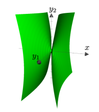
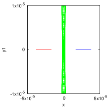
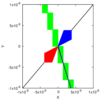
We now take T=26𝑇26T=26. The two rectangles in Figure 5 are the ΦT(Cpau,a)subscriptΦ𝑇𝐶superscriptsubscript𝑝𝑎𝑢𝑎\Phi_{T}\left(Cp_{a}^{u},a\right) for a=al𝑎subscript𝑎𝑙a=a_{l} and a=ar𝑎subscript𝑎𝑟a=a_{r} (see (24) for the definition of puusuperscriptsubscript𝑝𝑢𝑢p_{u}^{u}). Note that Figure 5 corresponds to the sketch from Figure 3. In Figure 5 we have the projection onto x,y1𝑥subscript𝑦1x,y_{1} coordinates of what happens inside of the set D𝐷D, without plotting the trajectory along the unstable manifold. Figure 6 presents the bounds, plotted in the original coordinates of the system.

We use the rigorous estimates for ΦT(Cpalu,al)subscriptΦ𝑇𝐶superscriptsubscript𝑝subscript𝑎𝑙𝑢subscript𝑎𝑙\Phi_{T}\left(Cp_{a_{l}}^{u},a_{l}\right) and ΦT(Cparu,ar)subscriptΦ𝑇𝐶superscriptsubscript𝑝subscript𝑎𝑟𝑢subscript𝑎𝑟\Phi_{T}\left(Cp_{a_{r}}^{u},a_{r}\right) to compute the following bounds (see (25) for the definition of the function hh,)

h(al)subscript𝑎𝑙\displaystyle h\left(a_{l}\right) [1.5093787863274e09,3.9653443827625e09],absent1.5093787863274𝑒093.9653443827625𝑒09\displaystyle\in[1.5093787863274e-09,3.9653443827625e-09],
h(ar)subscript𝑎𝑟\displaystyle h\left(a_{r}\right) [3.9570292285809e09,1.51777586447e09].absent3.9570292285809𝑒091.51777586447𝑒09\displaystyle\in\left[-3.9570292285809e-09,-1.51777586447e-09\right].

We also make sure that ΦT(Cpau,a)DsubscriptΦ𝑇𝐶superscriptsubscript𝑝𝑎𝑢𝑎𝐷\Phi_{T}\left(Cp_{a}^{u},a\right)\in D for all aA𝑎𝐴a\in A. We see that assumption (26) of Theorem 8 is satisfied, which means that we have a homoclinic connection for at least one of the parameters aA𝑎𝐴a\in A.

We have thus established a homoclinic orbit

(X0(t),Y0(t),Z0(t))=Φt(Cpa0u,a0),subscript𝑋0𝑡subscript𝑌0𝑡subscript𝑍0𝑡subscriptΦ𝑡𝐶superscriptsubscript𝑝subscript𝑎0𝑢subscript𝑎0\left(X_{0}(t),Y_{0}(t),Z_{0}(t)\right)=\Phi_{t}\left(Cp_{a_{0}}^{u},a_{0}\right),

for some a0Asubscript𝑎0𝐴a_{0}\in A.

Refer to caption
Refer to caption
Refer to caption
Figure 5: The bound on Wassuperscriptsubscript𝑊𝑎𝑠W_{a}^{s}, for all parameters a𝑎a. On the left we have a non-rigorous plot, to illustrate the shape of our bound in three dimensions. In the middle and on the right, we have a projection onto the x,y1𝑥subscript𝑦1x,y_{1} coordinates of the rigorous, computer assisted enclosure. The two rectangles depicted on the right hand side plots are ΦT(palu,al)subscriptΦ𝑇superscriptsubscript𝑝subscript𝑎𝑙𝑢subscript𝑎𝑙\Phi_{T}\left(p_{a_{l}}^{u},a_{l}\right) (on the left, in red) and ΦT(paru,ar)subscriptΦ𝑇superscriptsubscript𝑝subscript𝑎𝑟𝑢subscript𝑎𝑟\Phi_{T}\left(p_{a_{r}}^{u},a_{r}\right) (on the right, in blue). All these plots are in the local coordinates.
Refer to caption
Refer to caption
Figure 6: The bound on Wausuperscriptsubscript𝑊𝑎𝑢W_{a}^{u}, for all parameters a[al,ar]𝑎subscript𝑎𝑙subscript𝑎𝑟a\in[a_{l},a_{r}] on the left (in black). On the right, we have the bound on Wausuperscriptsubscript𝑊𝑎𝑢W_{a}^{u} in black, valid for all a[al,ar]𝑎subscript𝑎𝑙subscript𝑎𝑟a\in[a_{l},a_{r}]. A trajectory along Wausuperscriptsubscript𝑊𝑎𝑢W_{a}^{u}, which leaves the neighbourhood by the top right corner, returns through the lower edge of the plot. In red, we have the Walusuperscriptsubscript𝑊subscript𝑎𝑙𝑢W_{a_{l}}^{u}, as it returns to the neighbourhood, and in blue we have Warusuperscriptsubscript𝑊subscript𝑎𝑟𝑢W_{a_{r}}^{u}. In green is the bound on Wassuperscriptsubscript𝑊𝑎𝑠W_{a}^{s}, for all parameters a[al,ar]𝑎subscript𝑎𝑙subscript𝑎𝑟a\in[a_{l},a_{r}]. The bound on Wassuperscriptsubscript𝑊𝑎𝑠W_{a}^{s} in local coordinates is in fact is much tighter than on this plot. It is a strip that passes through the intersections of the green rectangles. The plots are in the original coordinates of the system, projected onto the X,Y𝑋𝑌X,Y coordinates.

The computer assisted proof has been done entirely by using the CAPD111computer assisted proofs in dynamics: http://capd.ii.uj.edu.pl/ package and took under a second on a single core 3Ghz Intel i7 processor.

4 Computation of the separatrix value

In this section we will show how we prove Theorem 6. First we will describe the method. We shall investigate the following ODE

γ(t)=(A+B(t))γ(t),superscript𝛾𝑡𝐴𝐵𝑡𝛾𝑡\gamma^{\prime}\left(t\right)=\left(A+B\left(t\right)\right)\gamma\left(t\right), (37)

and assume that a22,a33>0subscript𝑎22subscript𝑎330a_{22},a_{33}>0 and that

A=(0000a22000a33),B(t)=(b11(t)b12(t)b13(t)b21(t)b22(t)b23(t)b31(t)b32(t)b33(t)).formulae-sequence𝐴0000subscript𝑎22000subscript𝑎33𝐵𝑡subscript𝑏11𝑡subscript𝑏12𝑡subscript𝑏13𝑡subscript𝑏21𝑡subscript𝑏22𝑡subscript𝑏23𝑡subscript𝑏31𝑡subscript𝑏32𝑡subscript𝑏33𝑡A=\left(\begin{array}[]{lll}0&0&0\\ 0&-a_{22}&0\\ 0&0&-a_{33}\end{array}\right),\qquad B\left(t\right)=\left(\begin{array}[]{lll}b_{11}\left(t\right)&b_{12}\left(t\right)&b_{13}\left(t\right)\\ b_{21}\left(t\right)&b_{22}\left(t\right)&b_{23}\left(t\right)\\ b_{31}\left(t\right)&b_{32}\left(t\right)&b_{33}\left(t\right)\end{array}\right).

We assume also that there exist constants cb,λ>0subscript𝑐𝑏𝜆0c_{b},\lambda>0 for which

|bij(t)|cbeλ|t|.subscript𝑏𝑖𝑗𝑡subscript𝑐𝑏superscript𝑒𝜆𝑡|b_{ij}(t)|\leq c_{b}e^{-\lambda\left|t\right|}. (38)
Remark 16.

In section 4.3, where we will apply the method to the Shimizu-Marioka system (12), the constant cbsubscript𝑐𝑏c_{b} from (38) will be associated with the constant c𝑐c from Theorem 5, with the size of the neighborhood of zero in which we investigate the rate of convergence along the homoclinic, and also on some coordinate changes.

Remark 17.

Equation (37) can be seen as (16) considered in appropriate local coordinates. This will be our approach when applying the results from this section for the proof of Theorem 6.

In the sequel in our investigations of the problem (37) we will use the variables (x,y1,y2)𝑥subscript𝑦1subscript𝑦2(x,y_{1},y_{2}) and quite often we will also write y=(y1,y2)𝑦subscript𝑦1subscript𝑦2y=(y_{1},y_{2}), so that our coordinates will be (x,y)𝑥𝑦(x,y), where x𝑥x\in\mathbb{R} and y2𝑦superscript2y\in\mathbb{R}^{2}.

Our objective will be to obtain a proof of an orbit γ(t)superscript𝛾𝑡\gamma^{\ast}\left(t\right) of (37) for which

limtγ(t)subscript𝑡superscript𝛾𝑡\displaystyle\lim_{t\rightarrow-\infty}\gamma^{\ast}\left(t\right) =(x,0,0),absentsuperscriptsubscript𝑥00\displaystyle=(x_{-}^{\ast},0,0), (39)
limt+γ(t)subscript𝑡superscript𝛾𝑡\displaystyle\lim_{t\rightarrow+\infty}\gamma^{\ast}\left(t\right) =(x+,0,0),absentsuperscriptsubscript𝑥00\displaystyle=(x_{+}^{\ast},0,0), (40)

and also to obtain explicit bounds on the fraction x+xsuperscriptsubscript𝑥superscriptsubscript𝑥\frac{x_{+}^{\ast}}{x_{-}^{\ast}}.

To understand the behavior of (37) for large |t|𝑡|t|, we treat the line {(x,0,0),x}𝑥00𝑥\{(x,0,0),\,x\in\mathbb{R}\} as the normally hyperbolic manifold, with two stable directions (y1subscript𝑦1y_{1} and y2subscript𝑦2y_{2}). This is clearly visible in (37) with B0𝐵0B\equiv 0, but for |t|𝑡|t| large B𝐵B is just a small perturbation so the normally hyperbolic behavior will survive. A bit problematic in this picture is the fact that we have here an non-autonomous system, so the above scenario needs some adjustments. This is the idea, which underlines our approach.

Definition 18.

Let Z×2𝑍superscript2Z\subset\mathbb{R}\times\mathbb{R}^{2} and J𝐽J\subset\mathbb{R}. Let V:Z:𝑉𝑍V:Z\rightarrow\mathbb{R} be a C1superscript𝐶1C^{1} function. We say that V𝑉V is a Lyapunov function on J×Z𝐽𝑍J\times Z for (37) if for any solution z:J×2:𝑧𝐽superscript2z:J\rightarrow\mathbb{R}\times\mathbb{R}^{2} of (37), V(z(t))𝑉𝑧𝑡V(z(t)) is decreasing (ddtV(z(t))<0𝑑𝑑𝑡𝑉𝑧𝑡0\frac{d}{dt}V(z(t))<0) for z(t)Z𝑧𝑡𝑍z(t)\in Z and tJ𝑡𝐽t\in J.

We have

ddtV(z(t))=((A+B(t))z(t)|V(z(t))).𝑑𝑑𝑡𝑉𝑧𝑡conditional𝐴𝐵𝑡𝑧𝑡𝑉𝑧𝑡\frac{d}{dt}V(z(t))=((A+B(t))z(t)|\nabla V(z(t))). (41)

We start with two technical lemmas:

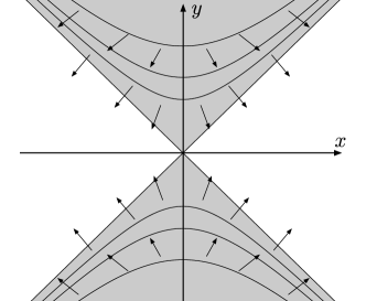
Refer to caption
Figure 7: The set D𝐷D from Lemma 19 is the vertical cone. The curved lines are the level sets of V𝑉V. The arrows indicate the vector field of (37).
Lemma 19.

Let D={y2x2}{0}𝐷superscriptnorm𝑦2superscript𝑥20D=\left\{\left\|y\right\|^{2}\geq x^{2}\right\}\setminus\{0\} (see Figure 7). Let J𝐽J\subset\mathbb{R} be a set of all t𝑡t\in\mathbb{R}, for which the following condition holds

6cbeλ|t|<min(a22,a33).6subscript𝑐𝑏superscript𝑒𝜆𝑡subscript𝑎22subscript𝑎336c_{b}e^{-\lambda\left|t\right|}<\min\left(a_{22},a_{33}\right). (42)

Then

V𝑉\displaystyle V :×2,:absentsuperscript2\displaystyle:\mathbb{R\times R}^{2}\rightarrow\mathbb{R},
V(x,y)𝑉𝑥𝑦\displaystyle V\left(x,y\right) =y2x2absentsuperscriptnorm𝑦2superscript𝑥2\displaystyle=\left\|y\right\|^{2}-x^{2}

is a Lyapunov function for (37) on J×D𝐽𝐷J\times D.

Proof.

For p=(x,y1,y2)𝑝𝑥subscript𝑦1subscript𝑦2p=\left(x,y_{1},y_{2}\right) we compute (skipping the dependence of bij(t)subscript𝑏𝑖𝑗𝑡b_{ij}(t) on t𝑡t to simplify the notation):

((A+B(t))p|12V(p))conditional𝐴𝐵𝑡𝑝12𝑉𝑝\displaystyle\left(\left(A+B\left(t\right)\right)p|\frac{1}{2}\nabla V\left(p\right)\right)
=\displaystyle= x2b11+y12(b22a22)+y22(b33a33)superscript𝑥2subscript𝑏11superscriptsubscript𝑦12subscript𝑏22subscript𝑎22superscriptsubscript𝑦22subscript𝑏33subscript𝑎33\displaystyle-x^{2}b_{11}+y_{1}^{2}\left(b_{22}-a_{22}\right)+y_{2}^{2}\left(b_{33}-a_{33}\right)
+xy1(b21b12)+xy2(b31b13)+y1y2(b23+b32)𝑥subscript𝑦1subscript𝑏21subscript𝑏12𝑥subscript𝑦2subscript𝑏31subscript𝑏13subscript𝑦1subscript𝑦2subscript𝑏23subscript𝑏32\displaystyle+xy_{1}\left(b_{21}-b_{12}\right)+xy_{2}\left(b_{31}-b_{13}\right)+y_{1}y_{2}\left(b_{23}+b_{32}\right)
\displaystyle\leq y2|b11|+(y12+y22)(max(|b22|,|b33|)+max(a22,a33))superscriptnorm𝑦2subscript𝑏11superscriptsubscript𝑦12superscriptsubscript𝑦22subscript𝑏22subscript𝑏33subscript𝑎22subscript𝑎33\displaystyle\left\|y\right\|^{2}\left|b_{11}\right|+\left(y_{1}^{2}+y_{2}^{2}\right)\left(\max\left(\left|b_{22}\right|,\left|b_{33}\right|\right)+\max\left(-a_{22},-a_{33}\right)\right)
+12(x2+y12)(|b21|+|b12|)+12(x2+y22)(|b31|+|b13|)12superscript𝑥2superscriptsubscript𝑦12subscript𝑏21subscript𝑏1212superscript𝑥2superscriptsubscript𝑦22subscript𝑏31subscript𝑏13\displaystyle+\frac{1}{2}\left(x^{2}+y_{1}^{2}\right)\left(\left|b_{21}\right|+\left|b_{12}\right|\right)+\frac{1}{2}\left(x^{2}+y_{2}^{2}\right)\left(\left|b_{31}\right|+\left|b_{13}\right|\right)
+12(y12+y22)(|b23|+|b32|)12superscriptsubscript𝑦12superscriptsubscript𝑦22subscript𝑏23subscript𝑏32\displaystyle\qquad+\frac{1}{2}\left(y_{1}^{2}+y_{2}^{2}\right)\left(\left|b_{23}\right|+\left|b_{32}\right|\right)
\displaystyle\leq [2cbeλ|t|+max(a22,a33)]y2delimited-[]2subscript𝑐𝑏superscript𝑒𝜆𝑡subscript𝑎22subscript𝑎33superscriptnorm𝑦2\displaystyle\left[2c_{b}e^{-\lambda\left|t\right|}+\max\left(-a_{22},-a_{33}\right)\right]\left\|y\right\|^{2}
+cbeλ|t|((x2+y12)+(x2+y22)+(y12+y22))subscript𝑐𝑏superscript𝑒𝜆𝑡superscript𝑥2superscriptsubscript𝑦12superscript𝑥2superscriptsubscript𝑦22superscriptsubscript𝑦12superscriptsubscript𝑦22\displaystyle+c_{b}e^{-\lambda\left|t\right|}\left(\left(x^{2}+y_{1}^{2}\right)+\left(x^{2}+y_{2}^{2}\right)+\left(y_{1}^{2}+y_{2}^{2}\right)\right)
\displaystyle\leq [2cbeλ|t|+max(a22,a33)]y2+cbeλ|t|(4y2)delimited-[]2subscript𝑐𝑏superscript𝑒𝜆𝑡subscript𝑎22subscript𝑎33superscriptnorm𝑦2subscript𝑐𝑏superscript𝑒𝜆𝑡4superscriptnorm𝑦2\displaystyle\left[2c_{b}e^{-\lambda\left|t\right|}+\max\left(-a_{22},-a_{33}\right)\right]\left\|y\right\|^{2}+c_{b}e^{-\lambda\left|t\right|}\left(4\left\|y\right\|^{2}\right)
=\displaystyle= [6cbeλ|t|min(a22,a33)]y2delimited-[]6subscript𝑐𝑏superscript𝑒𝜆𝑡subscript𝑎22subscript𝑎33superscriptnorm𝑦2\displaystyle\left[6c_{b}e^{-\lambda\left|t\right|}-\min\left(a_{22},a_{33}\right)\right]\left\|y\right\|^{2}
<\displaystyle< 0,0\displaystyle 0,

which concludes the proof. ∎

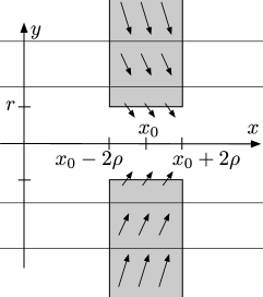
Refer to caption
Figure 8: The set D𝐷D from Lemma 20 is represented by the two shaded rectangular strips. The horizontal lines are the level sets of V𝑉V. The arrows indicate the vector field of (37).
Lemma 20.

Let x0,ρ,r>0subscript𝑥0𝜌𝑟0x_{0},\rho,r>0 and let

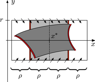
D=[x02ρ,x0+2ρ]×{yr}×2.𝐷subscript𝑥02𝜌subscript𝑥02𝜌norm𝑦𝑟superscript2D=\left[x_{0}-2\rho,x_{0}+2\rho\right]\times\left\{\left\|y\right\|\geq r\right\}\subset\mathbb{R\times R}^{2}.

Let J𝐽J be a set of t𝑡t\in\mathbb{R}, such that

2cbeλ|t|(1+x0+2ρr)<min(a22,a33),2subscript𝑐𝑏superscript𝑒𝜆𝑡1subscript𝑥02𝜌𝑟subscript𝑎22subscript𝑎332c_{b}e^{-\lambda\left|t\right|}\left(1+\frac{x_{0}+2\rho}{r}\right)<\min\left(a_{22},a_{33}\right), (43)

then

V𝑉\displaystyle V :×2,:absentsuperscript2\displaystyle:\mathbb{R\times R}^{2}\rightarrow\mathbb{R},
V(x,y)𝑉𝑥𝑦\displaystyle V\left(x,y\right) =y2absentsuperscriptnorm𝑦2\displaystyle=\left\|y\right\|^{2}

is a Lyapunov function for (37) on the set J×D𝐽𝐷J\times D.

Proof.

Let p=(x,y1,y2)𝑝𝑥subscript𝑦1subscript𝑦2p=\left(x,y_{1},y_{2}\right) and let R2=y12+y22rsuperscript𝑅2superscriptsubscript𝑦12superscriptsubscript𝑦22𝑟R^{2}=y_{1}^{2}+y_{2}^{2}\geq r. Note that ±y1y212R2plus-or-minussubscript𝑦1subscript𝑦212superscript𝑅2\pm y_{1}y_{2}\leq\frac{1}{2}R^{2} and |y1|,|y2|Rsubscript𝑦1subscript𝑦2𝑅\left|y_{1}\right|,\left|y_{2}\right|\leq R. We can compute (skipping the dependence of bij(t)subscript𝑏𝑖𝑗𝑡b_{ij}(t) on t𝑡t to simplify the notation)

((A+B(t))p|12V(p))conditional𝐴𝐵𝑡𝑝12𝑉𝑝\displaystyle\left(\left(A+B\left(t\right)\right)p|\frac{1}{2}\nabla V\left(p\right)\right)
=(a22+b22)y12+(a33+b33)y22absentsubscript𝑎22subscript𝑏22superscriptsubscript𝑦12subscript𝑎33subscript𝑏33superscriptsubscript𝑦22\displaystyle=\left(-a_{22}+b_{22}\right)y_{1}^{2}+\left(-a_{33}+b_{33}\right)y_{2}^{2}
+(b23+b32)y1y2+b21xy1+b31xy2subscript𝑏23subscript𝑏32subscript𝑦1subscript𝑦2subscript𝑏21𝑥subscript𝑦1subscript𝑏31𝑥subscript𝑦2\displaystyle\quad+\left(b_{23}+b_{32}\right)y_{1}y_{2}+b_{21}xy_{1}+b_{31}xy_{2}
max(a22+b22,a33+b33)R2absentsubscript𝑎22subscript𝑏22subscript𝑎33subscript𝑏33superscript𝑅2\displaystyle\leq\max\left(-a_{22}+b_{22},-a_{33}+b_{33}\right)R^{2}
+12(|b23|+|b32|)R2+|b21||x|R+|b31||x|R12subscript𝑏23subscript𝑏32superscript𝑅2subscript𝑏21𝑥𝑅subscript𝑏31𝑥𝑅\displaystyle\quad+\frac{1}{2}\left(\left|b_{23}\right|+\left|b_{32}\right|\right)R^{2}+\left|b_{21}\right|\left|x\right|R+\left|b_{31}\right|\left|x\right|R
(max(a22,a33)+2cbeλ|t|)R2+2cbeλ|t|(x0+2ρ)Rabsentsubscript𝑎22subscript𝑎332subscript𝑐𝑏superscript𝑒𝜆𝑡superscript𝑅22subscript𝑐𝑏superscript𝑒𝜆𝑡subscript𝑥02𝜌𝑅\displaystyle\leq\left(\max\left(-a_{22},-a_{33}\right)+2c_{b}e^{-\lambda\left|t\right|}\right)R^{2}+2c_{b}e^{-\lambda\left|t\right|}\left(x_{0}+2\rho\right)R
[max(a22,a33)+2cbeλ|t|(1+x0+2ρr)]R2absentdelimited-[]subscript𝑎22subscript𝑎332subscript𝑐𝑏superscript𝑒𝜆𝑡1subscript𝑥02𝜌𝑟superscript𝑅2\displaystyle\leq\left[\max\left(-a_{22},-a_{33}\right)+2c_{b}e^{-\lambda\left|t\right|}\left(1+\frac{x_{0}+2\rho}{r}\right)\right]R^{2}
<0,absent0\displaystyle<0,

as required. ∎

Let γ(t)𝛾𝑡\gamma\left(t\right) be the solution of (37) with initial condition γ(t0)=p𝛾subscript𝑡0𝑝\gamma\left(t_{0}\right)=p. We shall define

ϕt0,t(p):=γ(t0+t).assignsubscriptitalic-ϕsubscript𝑡0𝑡𝑝𝛾subscript𝑡0𝑡\phi_{t_{0},t}\left(p\right):=\gamma\left(t_{0}+t\right).

Note that

ddtϕt0,t(p)=(A+B(t0+t))ϕt0,t(p).𝑑𝑑𝑡subscriptitalic-ϕsubscript𝑡0𝑡𝑝𝐴𝐵subscript𝑡0𝑡subscriptitalic-ϕsubscript𝑡0𝑡𝑝\frac{d}{dt}\phi_{t_{0},t}\left(p\right)=\left(A+B\left(t_{0}+t\right)\right)\phi_{t_{0},t}\left(p\right). (44)
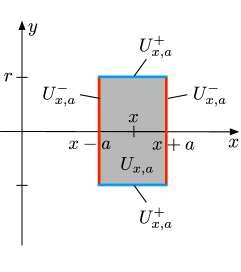
Definition 21.

Let r>0𝑟0r>0, a0𝑎0a\geq 0 and x𝑥x\in\mathbb{R} we define sets Ux,a,Ux,a+,Ux,a×2subscript𝑈𝑥𝑎superscriptsubscript𝑈𝑥𝑎superscriptsubscript𝑈𝑥𝑎superscript2U_{x,a},U_{x,a}^{+},U_{x,a}^{-}\subset\mathbb{R}\times\mathbb{R}^{2} by (see Figure 9)

Ux,asubscript𝑈𝑥𝑎\displaystyle U_{x,a} =[xa,x+a]×B¯(0,r),absent𝑥𝑎𝑥𝑎¯𝐵0𝑟\displaystyle=\left[x-a,x+a\right]\times\overline{B}(0,r),
Ux,a+superscriptsubscript𝑈𝑥𝑎\displaystyle U_{x,a}^{+} =[xa,x+a]×B¯(0,r),absent𝑥𝑎𝑥𝑎¯𝐵0𝑟\displaystyle=\left[x-a,x+a\right]\times\partial\overline{B}(0,r),
Ux,asuperscriptsubscript𝑈𝑥𝑎\displaystyle U_{x,a}^{-} =[xa,x+a]×B¯(0,r).absent𝑥𝑎𝑥𝑎¯𝐵0𝑟\displaystyle=\partial\left[x-a,x+a\right]\times\overline{B}(0,r).
Refer to caption
Figure 9: The sets Ux,asubscript𝑈𝑥𝑎U_{x,a}, Ux,a+superscriptsubscript𝑈𝑥𝑎U_{x,a}^{+} and Ux,asuperscriptsubscript𝑈𝑥𝑎U_{x,a}^{-}.

4.1 Behavior for t𝑡t\to-\infty

Below lemma allows us to obtain a bound on xsuperscriptsubscript𝑥x_{-}^{\ast} from (39). The idea is to choose some xsuperscript𝑥x^{\ast}\in\mathbb{R} and an initial condition in Ux,0subscript𝑈superscript𝑥0U_{x^{\ast},0} at an initial time t<0superscript𝑡0t^{\ast}<0. If tsuperscript𝑡t^{\ast} is small enough, then the influence of the matrix B(t)𝐵𝑡B\left(t\right) on (37) will be small.

Lemma 22.

Let us fix x>0superscript𝑥0x^{\ast}>0, ρ>0𝜌0\rho>0, r>0𝑟0r>0 and t<0superscript𝑡0t^{\ast}<0, such that conditions (42), (43) hold true for x0=xsubscript𝑥0superscript𝑥x_{0}=x^{\ast}. If

1λcbeλ|t|(x+2ρ+2r)<ρ,1𝜆subscript𝑐𝑏superscript𝑒𝜆superscript𝑡superscript𝑥2𝜌2𝑟𝜌\frac{1}{\lambda}c_{b}e^{-\lambda\left|t^{\ast}\right|}\left(x^{\ast}+2\rho+2r\right)<\rho, (45)

then there exists a unique point pUx,0superscript𝑝subscript𝑈superscript𝑥0p^{\ast}\in U_{x^{\ast},0} such that ϕt,t(p)subscriptitalic-ϕsuperscript𝑡𝑡superscript𝑝\phi_{t^{\ast},t}\left(p^{\ast}\right) is convergent as t𝑡t\rightarrow-\infty. Moreover,

limtϕt,t(p)=(x,0,0)Ux,ρ.subscript𝑡subscriptitalic-ϕsuperscript𝑡𝑡superscript𝑝superscriptsubscript𝑥00subscript𝑈superscript𝑥𝜌\lim_{t\rightarrow-\infty}\phi_{t^{\ast},t}\left(p^{\ast}\right)=\left(x_{-}^{\ast},0,0\right)\in U_{x^{\ast},\rho}.
Proof.

Since (43) holds for tsuperscript𝑡t^{\ast}, by Lemma 20 we see that Ux,2ρ+superscriptsubscript𝑈superscript𝑥2𝜌U_{x^{\ast},2\rho}^{+} is an “entry set” for the set Ux,2ρsubscript𝑈superscript𝑥2𝜌U_{x^{\ast},2\rho} (see Figures 8 ,9). What we mean by this statement is that for pUx,2ρ𝑝subscript𝑈superscript𝑥2𝜌p\in U_{x^{\ast},2\rho} and any t0<tsubscript𝑡0superscript𝑡t_{0}<t^{\ast} the trajectory ϕt0,s(p)subscriptitalic-ϕsubscript𝑡0𝑠𝑝\phi_{t_{0},s}(p) can not leave the set Ux,2ρsubscript𝑈superscript𝑥2𝜌U_{x^{\ast},2\rho} by passing through Ux,2ρ+superscriptsubscript𝑈superscript𝑥2𝜌U_{x^{\ast},2\rho}^{+} going forwards in time for s[0,tt0]𝑠0superscript𝑡subscript𝑡0s\in\left[0,t^{\ast}-t_{0}\right]. The only way it can exit is by passing through Ux,2ρsuperscriptsubscript𝑈superscript𝑥2𝜌U_{x^{\ast},2\rho}^{-}.

We will now show that for pUx,ρ𝑝subscript𝑈superscript𝑥𝜌p\in U_{x^{\ast},\rho} and any t0<tsubscript𝑡0superscript𝑡t_{0}<t^{\ast}, the trajectory ϕt0,s(p)subscriptitalic-ϕsubscript𝑡0𝑠𝑝\phi_{t_{0},s}(p) will never leave Ux,2ρsubscript𝑈superscript𝑥2𝜌U_{x^{\ast},2\rho} for s[0,tt0]𝑠0superscript𝑡subscript𝑡0s\in\left[0,t^{\ast}-t_{0}\right]. Since we can not exit through Ux,2ρ+superscriptsubscript𝑈superscript𝑥2𝜌U_{x^{\ast},2\rho}^{+}, we need to take care so that for s[0,tt0]𝑠0superscript𝑡subscript𝑡0s\in\left[0,t^{\ast}-t_{0}\right] the ϕt0,s(p)subscriptitalic-ϕsubscript𝑡0𝑠𝑝\phi_{t_{0},s}(p) does not reach Ux,2ρsuperscriptsubscript𝑈superscript𝑥2𝜌U_{x^{\ast},2\rho}^{-}. Let us use the notation

ϕt0,s(p)=(x(s),y1(s),y2(s)),subscriptitalic-ϕsubscript𝑡0𝑠𝑝𝑥𝑠subscript𝑦1𝑠subscript𝑦2𝑠\phi_{t_{0},s}\left(p\right)=\left(x\left(s\right),y_{1}\left(s\right),y_{2}\left(s\right)\right),

As long as |πxϕt0,t(p)x|2ρsubscript𝜋𝑥subscriptitalic-ϕsubscript𝑡0𝑡𝑝superscript𝑥2𝜌\left|\pi_{x}\phi_{t_{0},t}\left(p\right)-x^{\ast}\right|\leq 2\rho for t[0,s]𝑡0𝑠t\in\left[0,s\right], we have the following bound (using (45) in the last inequality)

|πxϕt0,s(p)x|subscript𝜋𝑥subscriptitalic-ϕsubscript𝑡0𝑠𝑝superscript𝑥\displaystyle\left|\pi_{x}\phi_{t_{0},s}\left(p\right)-x^{\ast}\right|
|πxpx|+|0sb11(t0+t)x(t)+b12(t0+t)y1(t)+b13(t0+t)y2(t)dt|absentsubscript𝜋𝑥𝑝superscript𝑥superscriptsubscript0𝑠subscript𝑏11subscript𝑡0𝑡𝑥𝑡subscript𝑏12subscript𝑡0𝑡subscript𝑦1𝑡subscript𝑏13subscript𝑡0𝑡subscript𝑦2𝑡𝑑𝑡\displaystyle\leq\left|\pi_{x}p-x^{\ast}\right|+\left|\int_{0}^{s}b_{11}\left(t_{0}+t\right)x\left(t\right)+b_{12}\left(t_{0}+t\right)y_{1}\left(t\right)+b_{13}\left(t_{0}+t\right)y_{2}\left(t\right)dt\right|
ρ+tt0cbeλ(t0+t)(x+2ρ+2r)𝑑tabsent𝜌superscriptsubscriptsuperscript𝑡subscript𝑡0subscript𝑐𝑏superscript𝑒𝜆subscript𝑡0𝑡superscript𝑥2𝜌2𝑟differential-d𝑡\displaystyle\leq\rho+\int_{-\infty}^{t^{\ast}-t_{0}}c_{b}e^{\lambda\left(t_{0}+t\right)}\left(x^{\ast}+2\rho+2r\right)dt
=ρ+1λcbeλt(x+2ρ+2r)absent𝜌1𝜆subscript𝑐𝑏superscript𝑒𝜆superscript𝑡superscript𝑥2𝜌2𝑟\displaystyle=\rho+\frac{1}{\lambda}c_{b}e^{\lambda t^{\ast}}\left(x^{\ast}+2\rho+2r\right)
<c^2ρ,absent^𝑐2𝜌\displaystyle<\hat{c}2\rho, (46)

for a fixed c^(12,1)^𝑐121\hat{c}\in\left(\frac{1}{2},1\right), which does not depend on s𝑠s.

t0t,s[0,tt0],πxϕt0,s(p)x2ρ.formulae-sequencefor-allsubscript𝑡0superscript𝑡formulae-sequencefor-all𝑠0superscript𝑡subscript𝑡0normsubscript𝜋𝑥subscriptitalic-ϕsubscript𝑡0𝑠𝑝superscript𝑥2𝜌\forall t_{0}\leq t^{\ast},\ \forall s\in[0,t^{\ast}-t_{0}],\qquad\quad\|\pi_{x}\phi_{t_{0},s}(p)-x^{\ast}\|\leq 2\rho.

This shows that ϕt0,ssubscriptitalic-ϕsubscript𝑡0𝑠\phi_{t_{0},s} will not leave Ux,2ρ.subscript𝑈superscript𝑥2𝜌U_{x^{\ast},2\rho}. Since trajectories from Ux,ρsubscript𝑈superscript𝑥𝜌U_{x^{\ast},\rho} do not leave Ux,2ρsubscript𝑈superscript𝑥2𝜌U_{x^{\ast},2\rho} and can not touch Ux,2ρ+superscriptsubscript𝑈superscript𝑥2𝜌U_{x^{\ast},2\rho}^{+}, we have established that

t0<t,s(0,tt0],ϕt0,s(Ux,ρ)intUx,2ρ.formulae-sequencefor-allsubscript𝑡0superscript𝑡formulae-sequencefor-all𝑠0superscript𝑡subscript𝑡0subscriptitalic-ϕsubscript𝑡0𝑠subscript𝑈superscript𝑥𝜌intsubscript𝑈superscript𝑥2𝜌\forall t_{0}<t^{\ast},\ \forall s\in(0,t^{\ast}-t_{0}],\qquad\phi_{t_{0},s}(U_{x^{\ast},\rho})\subset\mathrm{int}U_{x^{\ast},2\rho}. (47)

Mirror estimates to (46) together with (45) lead to

|πxϕt0,s(p)πxp|1λcbeλt(x+2ρ+2r)<ρ,subscript𝜋𝑥subscriptitalic-ϕsubscript𝑡0𝑠𝑝subscript𝜋𝑥𝑝1𝜆subscript𝑐𝑏superscript𝑒𝜆superscript𝑡superscript𝑥2𝜌2𝑟𝜌|\pi_{x}\phi_{t_{0},s}(p)-\pi_{x}p|\leq\frac{1}{\lambda}c_{b}e^{\lambda t^{\ast}}(x^{\ast}+2\rho+2r)<\rho,

hence we proved that

|πxϕt0,s(p)πxp|<ρ,t0<tpUx,ρs[0,tt0].formulae-sequencesubscript𝜋𝑥subscriptitalic-ϕsubscript𝑡0𝑠𝑝subscript𝜋𝑥𝑝𝜌for-allsubscript𝑡0superscript𝑡for-all𝑝subscript𝑈superscript𝑥𝜌for-all𝑠0superscript𝑡subscript𝑡0|\pi_{x}\phi_{t_{0},s}(p)-\pi_{x}p|<\rho,\quad\forall t_{0}<t^{\ast}\,\forall p\in U_{x^{\ast},\rho}\,\forall s\in[0,t^{\ast}-t_{0}]. (48)

In particular we obtain for any yB(0,r)¯𝑦¯𝐵0𝑟y\in\overline{B(0,r)}, for all t0tsubscript𝑡0superscript𝑡t_{0}\leq t^{\ast} and s[0,tt0]𝑠0superscript𝑡subscript𝑡0s\in[0,t^{\ast}-t_{0}]

πxϕt0,s(xρ,y)<x,πxϕt0,s(x+ρ,y)>x.formulae-sequencesubscript𝜋𝑥subscriptitalic-ϕsubscript𝑡0𝑠superscript𝑥𝜌𝑦superscript𝑥subscript𝜋𝑥subscriptitalic-ϕsubscript𝑡0𝑠superscript𝑥𝜌𝑦superscript𝑥\pi_{x}\phi_{t_{0},s}(x^{\ast}-\rho,y)<x^{\ast},\quad\pi_{x}\phi_{t_{0},s}(x^{\ast}+\rho,y)>x^{\ast}. (49)
Refer to caption
Figure 10: The set Ux,ρsubscript𝑈superscript𝑥𝜌U_{x^{\ast},\rho} in light grey and ϕt0,s(Ux,ρ)subscriptitalic-ϕsubscript𝑡0𝑠subscript𝑈superscript𝑥𝜌\phi_{t_{0},s}\left(U_{x^{\ast},\rho}\right) in dark grey. The set Ux,0subscript𝑈superscript𝑥0U_{x^{\ast},0} is represented by the dashed vertical line.

From (47) and (49), due to the topological alignment (see Figure 10) of the sets ϕt0,s(Ux,ρ)subscriptitalic-ϕsubscript𝑡0𝑠subscript𝑈superscript𝑥𝜌\phi_{t_{0},s}\left(U_{x^{\ast},\rho}\right) and Ux,0subscript𝑈superscript𝑥0U_{x^{\ast},0}, it follows that for any t0<tsubscript𝑡0superscript𝑡t_{0}<t^{\ast} there exist points q=q(t0)Ux,ρ𝑞𝑞subscript𝑡0subscript𝑈superscript𝑥𝜌q=q\left(t_{0}\right)\in U_{x^{\ast},\rho} and p=p(t0)Ux,0𝑝𝑝subscript𝑡0subscript𝑈superscript𝑥0p=p\left(t_{0}\right)\in U_{x^{\ast},0}, such that ϕt0,tt0(q)=psubscriptitalic-ϕsubscript𝑡0superscript𝑡subscript𝑡0𝑞𝑝\phi_{t_{0},t^{\ast}-t_{0}}\left(q\right)=p and ϕt0,s(q)Ux,2ρsubscriptitalic-ϕsubscript𝑡0𝑠𝑞subscript𝑈superscript𝑥2𝜌\phi_{t_{0},s}\left(q\right)\in U_{x^{\ast},2\rho} for s[0,tt0]𝑠0superscript𝑡subscript𝑡0s\in\left[0,t^{\ast}-t_{0}\right]. This implies that

ϕt,t0t(p)subscriptitalic-ϕsuperscript𝑡subscript𝑡0superscript𝑡𝑝\displaystyle\phi_{t^{\ast},t_{0}-t^{\ast}}\left(p\right) Ux,ρ,absentsubscript𝑈superscript𝑥𝜌\displaystyle\in U_{x^{\ast},\rho}, (50)
ϕt,s(p)subscriptitalic-ϕsuperscript𝑡𝑠𝑝\displaystyle\phi_{t^{\ast},s}\left(p\right) Ux,2ρfor s[t0t,0].formulae-sequenceabsentsubscript𝑈superscript𝑥2𝜌for 𝑠subscript𝑡0superscript𝑡0\displaystyle\in U_{x^{\ast},2\rho}\qquad\mathchoice{\hbox{{for }}}{\hbox{{\firstchoice@false for }}}{\hbox{{\firstchoice@false for }}}{\hbox{{\firstchoice@false for }}}s\in[t_{0}-t^{\ast},0].

Let pn=p(n)subscript𝑝𝑛𝑝𝑛p_{n}=p\left(-n\right) (by taking t0=nsubscript𝑡0𝑛t_{0}=-n).

Since Ux,0subscript𝑈superscript𝑥0U_{x^{\ast},0} is compact, we can pass to a convergent subsequence pnkpUx,0subscript𝑝subscript𝑛𝑘superscript𝑝subscript𝑈superscript𝑥0p_{n_{k}}\rightarrow p^{\ast}\in U_{x^{\ast},0}, and obtain a point for which

ϕt,s(p)Ux,2ρfor s(,0].formulae-sequencesubscriptitalic-ϕsuperscript𝑡𝑠superscript𝑝subscript𝑈superscript𝑥2𝜌for 𝑠0\phi_{t^{\ast},s}\left(p^{\ast}\right)\in U_{x^{\ast},2\rho}\qquad\mathchoice{\hbox{{for }}}{\hbox{{\firstchoice@false for }}}{\hbox{{\firstchoice@false for }}}{\hbox{{\firstchoice@false for }}}s\in(-\infty,0]. (51)

We now need to show that ϕt,s(p)subscriptitalic-ϕsuperscript𝑡𝑠superscript𝑝\phi_{t^{\ast},s}\left(p^{\ast}\right) is convergent as s𝑠s\rightarrow-\infty.

We first focus on the x𝑥x coordinate. We will show that for any ε𝜀\varepsilon, there exists an S<0𝑆0S<0, such that for any s1,s2<Ssubscript𝑠1subscript𝑠2𝑆s_{1},s_{2}<S holds (the Cauchy condition for the function sπxϕt,s1(p)maps-to𝑠subscript𝜋𝑥subscriptitalic-ϕsuperscript𝑡subscript𝑠1superscript𝑝s\mapsto\pi_{x}\phi_{t^{\ast},s_{1}}\left(p^{\ast}\right) for s𝑠s\rightarrow-\infty)

πxϕt,s1(p)πxϕt,s2(p)ε.normsubscript𝜋𝑥subscriptitalic-ϕsuperscript𝑡subscript𝑠1superscript𝑝subscript𝜋𝑥subscriptitalic-ϕsuperscript𝑡subscript𝑠2superscript𝑝𝜀\left\|\pi_{x}\phi_{t^{\ast},s_{1}}\left(p^{\ast}\right)-\pi_{x}\phi_{t^{\ast},s_{2}}\left(p^{\ast}\right)\right\|\leq\varepsilon. (52)

Assume that s1<s2subscript𝑠1subscript𝑠2s_{1}<s_{2} and that u=s1s2𝑢subscript𝑠1subscript𝑠2u=s_{1}-s_{2}. Then, by estimates analogous to (46),

πxϕt,s1(p)πxϕt,s2(p)normsubscript𝜋𝑥subscriptitalic-ϕsuperscript𝑡subscript𝑠1superscript𝑝subscript𝜋𝑥subscriptitalic-ϕsuperscript𝑡subscript𝑠2superscript𝑝\displaystyle\left\|\pi_{x}\phi_{t^{\ast},s_{1}}\left(p^{\ast}\right)-\pi_{x}\phi_{t^{\ast},s_{2}}\left(p^{\ast}\right)\right\|
=πxϕt,s2+u(p)πxϕt,s2(p)absentnormsubscript𝜋𝑥subscriptitalic-ϕsuperscript𝑡subscript𝑠2𝑢superscript𝑝subscript𝜋𝑥subscriptitalic-ϕsuperscript𝑡subscript𝑠2superscript𝑝\displaystyle=\left\|\pi_{x}\phi_{t^{\ast},s_{2}+u}\left(p^{\ast}\right)-\pi_{x}\phi_{t^{\ast},s_{2}}\left(p^{\ast}\right)\right\|
1λcbes2(x+2ρ+2r).absent1𝜆subscript𝑐𝑏superscript𝑒subscript𝑠2superscript𝑥2𝜌2𝑟\displaystyle\leq\frac{1}{\lambda}c_{b}e^{s_{2}}\left(x^{\ast}+2\rho+2r\right).

We see that by choosing negative s2subscript𝑠2s_{2}, with |s2|subscript𝑠2\left|s_{2}\right| sufficiently large, we obtain (52). This implies the existence of limsπxϕt,s1(p).subscript𝑠subscript𝜋𝑥subscriptitalic-ϕsuperscript𝑡subscript𝑠1superscript𝑝\lim_{s\rightarrow-\infty}\pi_{x}\phi_{t^{\ast},s_{1}}\left(p^{\ast}\right).

We will now show that

limsπyϕt,s(p)=0.subscript𝑠subscript𝜋𝑦subscriptitalic-ϕsuperscript𝑡𝑠superscript𝑝0\lim_{s\rightarrow-\infty}\pi_{y}\phi_{t^{\ast},s}\left(p^{\ast}\right)=0. (53)

Suppose that this is not the case. Thus, there would exist a δ𝛿\delta and a sequence sisubscript𝑠𝑖s_{i}\rightarrow-\infty such that

|πyϕt,si(p)|>δ.subscript𝜋𝑦subscriptitalic-ϕsuperscript𝑡subscript𝑠𝑖superscript𝑝𝛿\left|\pi_{y}\phi_{t^{\ast},s_{i}}\left(p^{\ast}\right)\right|>\delta.

Let us choose sisubscript𝑠𝑖s_{i} negative enough so that the V(x,y)=y2𝑉𝑥𝑦superscriptnorm𝑦2V\left(x,y\right)=\left\|y\right\|^{2} would be a Lyapunov function on J×D𝐽𝐷J\times D with J=(,si]𝐽subscript𝑠𝑖J=(-\infty,s_{i}] and

D=[x2ρ,x+2ρ]×{yδ2}.𝐷superscript𝑥2𝜌superscript𝑥2𝜌norm𝑦𝛿2D=\left[x^{\ast}-2\rho,x^{\ast}+2\rho\right]\times\left\{\left\|y\right\|\geq\frac{\delta}{2}\right\}.

This is possible, since we can apply Lemma 20 provided that condition (43) is satisfied. The (43) will hold for r=δ2𝑟𝛿2r=\frac{\delta}{2}, provided that t<T𝑡𝑇t<T, for T𝑇T negative enough. Since V𝑉V is a Lyapunov function, by going backward in time, for s<si<T𝑠subscript𝑠𝑖𝑇s<s_{i}<T, ϕt,ssubscriptitalic-ϕsuperscript𝑡𝑠\phi_{t^{\ast},s} will exit Ux,2ρsubscript𝑈superscript𝑥2𝜌U_{x^{\ast},2\rho}. This contradicts (51), hence

limsπyϕt,s(p)=0.subscript𝑠subscript𝜋𝑦subscriptitalic-ϕsuperscript𝑡𝑠superscript𝑝0\lim_{s\rightarrow-\infty}\pi_{y}\phi_{t^{\ast},s}\left(p^{\ast}\right)=0.

We have shown that ϕt,s(p)subscriptitalic-ϕsuperscript𝑡𝑠superscript𝑝\phi_{t^{\ast},s}\left(p^{\ast}\right) is convergent as s𝑠s\rightarrow-\infty, and that the limit lies in Ux,2ρsubscript𝑈superscript𝑥2𝜌U_{x^{\ast},2\rho}. The fact that the limit is in fact in Ux,ρsubscript𝑈superscript𝑥𝜌U_{x^{\ast},\rho} follows from (48).

We will now show that the point psuperscript𝑝p^{\ast} is unique. Suppose that we have a second point pUx,0superscript𝑝absentsubscript𝑈superscript𝑥0p^{\ast\ast}\in U_{x^{\ast},0} for which limsϕt,s(p)subscript𝑠subscriptitalic-ϕsuperscript𝑡𝑠superscript𝑝absent\lim_{s\rightarrow-\infty}\phi_{t^{\ast},s}\left(p^{\ast\ast}\right) exists. Consider the following time dependent change of coordinates (t+t,ξ=(t+t,x,y)ϕt,t(p))superscript𝑡𝑡𝜉superscript𝑡𝑡𝑥𝑦subscriptitalic-ϕsuperscript𝑡𝑡superscript𝑝(t^{\ast}+t,\xi=(t^{\ast}+t,x,y)-\phi_{t^{\ast},t}\left(p^{\ast}\right)), which means that we just continuously change the location of the origin, by subtracting some solution. Our equation is linear, hence in new coordinates the equation is the same, ξ=(A+B(t))ξsuperscript𝜉𝐴𝐵𝑡𝜉\xi^{\prime}=(A+B(t))\xi.

Let us take an initial condition ξ(t)=pp𝜉superscript𝑡superscript𝑝absentsuperscript𝑝\xi\left(t^{\ast}\right)=p^{\ast\ast}-p^{\ast}. If ppsuperscript𝑝absentsuperscript𝑝p^{\ast\ast}\neq p^{\ast}, since by construction p,pUx,0,superscript𝑝absentsuperscript𝑝subscript𝑈superscript𝑥0p^{\ast\ast},p^{\ast}\in U_{x^{\ast},0}, we see that ξ(t)D={y2>|x|}𝜉superscript𝑡𝐷superscriptnorm𝑦2𝑥\xi\left(t^{\ast}\right)\in D=\left\{\left\|y\right\|^{2}>\left|x\right|\right\}. Since we assumed that for tsuperscript𝑡t^{\ast} condition (42) holds, it also holds for all t<t𝑡superscript𝑡t<t^{\ast}. By Lemma 19, this means that for s<0,𝑠0s<0, ξ(t+s)𝜉superscript𝑡𝑠\xi\left(t^{\ast}+s\right) stays inside D𝐷D. Moreover, since V(x,y)=y2x𝑉𝑥𝑦superscriptnorm𝑦2𝑥V(x,y)=\left\|y\right\|^{2}-x is a Lyapunov function, ξ(t+s)𝜉superscript𝑡𝑠\xi\left(t^{\ast}+s\right) must tend to infinity as s𝑠s\rightarrow-\infty. Since ξ(t+s)=ϕt,s(p)ϕt,s(p)𝜉superscript𝑡𝑠subscriptitalic-ϕsuperscript𝑡𝑠superscript𝑝absentsubscriptitalic-ϕsuperscript𝑡𝑠superscript𝑝\xi\left(t^{\ast}+s\right)=\phi_{t^{\ast},s}\left(p^{\ast\ast}\right)-\phi_{t^{\ast},s}\left(p^{\ast}\right), this means that we can not have both ppsuperscript𝑝absentsuperscript𝑝p^{\ast\ast}\neq p^{\ast} and ϕt,s(p)subscriptitalic-ϕsuperscript𝑡𝑠superscript𝑝absent\phi_{t^{\ast},s}\left(p^{\ast\ast}\right) convergent. We have thus shown that psuperscript𝑝p^{\ast} is the only point in Ux,0subscript𝑈superscript𝑥0U_{x^{\ast},0} for which the limit exists. ∎

Corollary 23.

If we consider t=0superscript𝑡0t^{\ast}=0, x=1superscript𝑥1x^{\ast}=1, r=ρ𝑟𝜌r=\rho, and when

00\displaystyle 0 <\displaystyle< λ4cb,𝜆4subscript𝑐𝑏\displaystyle\lambda-4c_{b},
00\displaystyle 0 <\displaystyle< min(a22,a33)6cb,subscript𝑎22subscript𝑎336subscript𝑐𝑏\displaystyle\min\left(a_{22},a_{33}\right)-6c_{b},
r𝑟\displaystyle r >\displaystyle> max(cbλ4cb,2cbmin(a22,a33)6cb),subscript𝑐𝑏𝜆4subscript𝑐𝑏2subscript𝑐𝑏subscript𝑎22subscript𝑎336subscript𝑐𝑏\displaystyle\max\left(\frac{c_{b}}{\lambda-4c_{b}},\frac{2c_{b}}{\min\left(a_{22},a_{33}\right)-6c_{b}}\right),

then assumptions of Lemma 22 are satisfied.

4.2 Behavior for t𝑡t\to\infty

We now consider a point in Ux,0subscript𝑈superscript𝑥absent0U_{x^{\ast\ast},0} with initial time t>0superscript𝑡absent0t^{\ast\ast}>0.

Lemma 24.

Let us fix x>0superscript𝑥absent0x^{\ast\ast}>0, ρ>0𝜌0\rho>0, r>0𝑟0r>0 and t>0superscript𝑡absent0t^{\ast\ast}>0, such that conditions (42), (43) hold true for x0=xsubscript𝑥0superscript𝑥absentx_{0}=x^{\ast\ast}.

If

1λcbeλt(x+2ρ+2r)<ρ,1𝜆subscript𝑐𝑏superscript𝑒𝜆superscript𝑡absentsuperscript𝑥absent2𝜌2𝑟𝜌\frac{1}{\lambda}c_{b}e^{-\lambda t^{\ast\ast}}\left(x^{\ast\ast}+2\rho+2r\right)<\rho,

then for any pUx,0superscript𝑝absentsubscript𝑈superscript𝑥absent0p^{\ast\ast}\in U_{x^{\ast\ast},0} the ϕt,t(p)subscriptitalic-ϕsuperscript𝑡absent𝑡superscript𝑝absent\phi_{t^{\ast\ast},t}\left(p^{\ast\ast}\right) is convergent as t+𝑡t\rightarrow+\infty. Moreover,

limt+ϕt,t(p)=(x+,0,0)Ux,ρ.subscript𝑡subscriptitalic-ϕsuperscript𝑡absent𝑡superscript𝑝absentsuperscriptsubscript𝑥absent00subscript𝑈superscript𝑥absent𝜌\lim_{t\rightarrow+\infty}\phi_{t^{\ast\ast},t}\left(p^{\ast\ast}\right)=\left(x_{+}^{\ast\ast},0,0\right)\in U_{x^{\ast\ast},\rho}. (54)
Proof.

The proof follows analogous in steps as the proof of Lemma 22. Since (43) holds for tsuperscript𝑡t^{\ast}, by Lemma 20 we see that Ux,2ρ+superscriptsubscript𝑈superscript𝑥absent2𝜌U_{x^{\ast\ast},2\rho}^{+} is an “entry set” for the set Ux,2ρsubscript𝑈superscript𝑥absent2𝜌U_{x^{\ast\ast},2\rho} (see Figures 8 ,9). By a similar derivation to (46) we can establish that trajectories from Ux,0subscript𝑈superscript𝑥0U_{x^{\ast},0} do not leave Ux,ρsubscript𝑈superscript𝑥𝜌U_{x^{\ast},\rho},

ϕt,s(Ux,0)Ux,ρfor all s>0.formulae-sequencesubscriptitalic-ϕsuperscript𝑡absent𝑠subscript𝑈superscript𝑥0subscript𝑈superscript𝑥absent𝜌for all 𝑠0\phi_{t^{\ast\ast},s}(U_{x^{\ast},0})\subset U_{x^{\ast\ast},\rho}\qquad\mathchoice{\hbox{{for all }}}{\hbox{{\firstchoice@false for all }}}{\hbox{{\firstchoice@false for all }}}{\hbox{{\firstchoice@false for all }}}s>0.

Using the same method (but taking the limit to ++\infty instead of -\infty) as for the proof of (52) we can show that we have convergence of πxϕt,t(p)subscript𝜋𝑥subscriptitalic-ϕsuperscript𝑡absent𝑡superscript𝑝absent\pi_{x}\phi_{t^{\ast\ast},t}\left(p^{\ast\ast}\right) as t𝑡t goes to ++\infty for any pUx,0superscript𝑝absentsubscript𝑈superscript𝑥absent0p^{\ast\ast}\in U_{x^{\ast\ast},0}.

We need to show that

lims+πyϕt,s(p)=0.subscript𝑠subscript𝜋𝑦subscriptitalic-ϕsuperscript𝑡absent𝑠superscript𝑝absent0\lim_{s\rightarrow+\infty}\pi_{y}\phi_{t^{\ast\ast},s}\left(p^{\ast\ast}\right)=0. (55)

Suppose that this is not the case. Then there would exist a δ𝛿\delta and a sequence si+subscript𝑠𝑖s_{i}\rightarrow+\infty such that

|πyϕt,si(p)|>δ.subscript𝜋𝑦subscriptitalic-ϕsuperscript𝑡absentsubscript𝑠𝑖superscript𝑝absent𝛿\left|\pi_{y}\phi_{t^{\ast\ast},s_{i}}\left(p^{\ast\ast}\right)\right|>\delta. (56)

Let us choose T𝑇T positive enough so that V(x,y)=y2𝑉𝑥𝑦superscriptnorm𝑦2V\left(x,y\right)=\left\|y\right\|^{2} would be a Lyapunov function on [T,+)×D𝑇𝐷[T,+\infty)\times D, for

D=[x2ρ,x+2ρ]×{yδ2}.𝐷superscript𝑥absent2𝜌superscript𝑥absent2𝜌norm𝑦𝛿2D=\left[x^{\ast\ast}-2\rho,x^{\ast\ast}+2\rho\right]\times\left\{\left\|y\right\|\geq\frac{\delta}{2}\right\}.

This is possible, since we can apply Lemma 20 provided that condition (43) is satisfied. The (43) will hold for r=δ2𝑟𝛿2r=\frac{\delta}{2}, provided that T<t𝑇𝑡T<t, for T𝑇T large enough. Since V𝑉V is a Lyapunov function, by going forwards in time ϕt,s(p)subscriptitalic-ϕsuperscript𝑡absent𝑠superscript𝑝absent\phi_{t^{\ast\ast},s}\left(p^{\ast\ast}\right) will enter [x2ρ,x+2ρ]×{y<δ2}superscript𝑥absent2𝜌superscript𝑥absent2𝜌norm𝑦𝛿2\left[x^{\ast\ast}-2\rho,x^{\ast\ast}+2\rho\right]\times\left\{\left\|y\right\|<\frac{\delta}{2}\right\} and once it enters, it will remain there. This contradicts (56), hence we have established (55). ∎

Corollary 25.

Consider t=0superscript𝑡absent0t^{\ast\ast}=0. If

00\displaystyle 0 <\displaystyle< min(a22,a33)6cb,subscript𝑎22subscript𝑎336subscript𝑐𝑏\displaystyle\min\left(a_{22},a_{33}\right)-6c_{b},
00\displaystyle 0 <\displaystyle< λ2cb,𝜆2subscript𝑐𝑏\displaystyle\lambda-2c_{b},

and

ρ𝜌\displaystyle\rho <\displaystyle< 12[r(12cbmin(a22,a33)1)x],12delimited-[]𝑟12subscript𝑐𝑏subscript𝑎22subscript𝑎331superscript𝑥absent\displaystyle\frac{1}{2}\left[r\left(\frac{1}{2c_{b}}\min\left(a_{22},a_{33}\right)-1\right)-x^{\ast\ast}\right],
ρ𝜌\displaystyle\rho >\displaystyle> cb(x+2r)λ2cb,subscript𝑐𝑏superscript𝑥absent2𝑟𝜆2subscript𝑐𝑏\displaystyle\frac{c_{b}\left(x^{\ast\ast}+2r\right)}{\lambda-2c_{b}},

then assumptions of Lemma 24 are satisfied.

Lemmas 22, 24 lead to the following algorithm for establishing bounds for xsuperscriptsubscript𝑥x_{-}^{\ast} and x+superscriptsubscript𝑥x_{+}^{\ast}:

Algorithm 2:

  1. 1.

    Fix r,ρ>0𝑟𝜌0r,\rho>0 and choose t<0superscript𝑡0t^{\ast}<0 small enough to satisfy assumptions of Lemma 22. The Lemma 22 then ensures that

    x[xρ,x+ρ].superscriptsubscript𝑥superscript𝑥𝜌superscript𝑥𝜌x_{-}^{\ast}\in\left[x^{\ast}-\rho,x^{\ast}+\rho\right].
  2. 2.

    By rigorous numerical integration, evaluate the bound for ϕt,t(Ux,0).subscriptitalic-ϕsuperscript𝑡𝑡subscript𝑈superscript𝑥0\phi_{t^{\ast},t}(U_{x^{\ast},0}). The t>0𝑡0t>0 needs to be chosen large enough so that t=t+tsuperscript𝑡absentsuperscript𝑡𝑡t^{\ast\ast}=t^{\ast}+t satisfies assumptions of Lemma 24. The t𝑡t also needs to be large enough so that ϕt,t(Ux,0)Ux,bsubscriptitalic-ϕsuperscript𝑡𝑡subscript𝑈superscript𝑥0subscript𝑈superscript𝑥absent𝑏\phi_{t^{\ast},t}(U_{x^{\ast},0})\subset U_{x^{\ast\ast},b}, for some b>0𝑏0b>0.

  3. 3.

    By Lemma 24 limt+ϕt,t(p)Ux,b+ρsubscript𝑡subscriptitalic-ϕsuperscript𝑡𝑡superscript𝑝subscript𝑈superscript𝑥absent𝑏𝜌\lim_{t\rightarrow+\infty}\phi_{t^{\ast},t}\left(p^{\ast}\right)\in U_{x^{\ast\ast},b+\rho}. This ensures that

    x+[xbρ,x+b+ρ].superscriptsubscript𝑥superscript𝑥absent𝑏𝜌superscript𝑥absent𝑏𝜌x_{+}^{\ast}\in\left[x^{\ast\ast}-b-\rho,x^{\ast\ast}+b+\rho\right].

    We then have the following bound:

    x+x[xbρx+ρ,x+b+ρxρ].superscriptsubscript𝑥superscriptsubscript𝑥superscript𝑥absent𝑏𝜌superscript𝑥𝜌superscript𝑥absent𝑏𝜌superscript𝑥𝜌\frac{x_{+}^{\ast}}{x_{-}^{\ast}}\in\left[\frac{x^{\ast\ast}-b-\rho}{x^{\ast}+\rho},\frac{x^{\ast\ast}+b+\rho}{x^{\ast}-\rho}\right].

4.3 Application to the Shimizu Morioka system

In this section we prove Theorem 6. We will consider a matrix P𝑃P consisting of the eigenvectors of (17), of the form

P=(1a0+10110001).𝑃1subscript𝑎010110001P=\left(\begin{array}[]{lll}1&a_{0}+1&0\\ -1&1&0\\ 0&0&1\end{array}\right). (57)

Thus, P𝑃P is transition from the eigenvectors basis to the standard one. In coordinates γ𝛾\gamma given by η=Pγ𝜂𝑃𝛾\eta=P\gamma, the ODE (16) takes form

γ=(A+B(t))γ,superscript𝛾𝐴𝐵𝑡𝛾\gamma^{\prime}=\left(A+B\left(t\right)\right)\gamma, (58)

for

A𝐴\displaystyle A =\displaystyle= (0000(a0+2)000a0).0000subscript𝑎02000subscript𝑎0\displaystyle\left(\begin{array}[]{ccc}0&0&0\\ 0&-\left(a_{0}+2\right)&0\\ 0&0&-a_{0}\end{array}\right). (62)
B(t)𝐵𝑡\displaystyle B\left(t\right) =\displaystyle= a0+1a0+2(Z0(t)Z0(t)2X0(t)a0+1Z0(t)Z0(t)2X0(t)a0+1(a0+2)X0(t)(a0+2)X0(t)0).subscript𝑎01subscript𝑎02subscript𝑍0𝑡subscript𝑍0𝑡2subscript𝑋0𝑡subscript𝑎01subscript𝑍0𝑡subscript𝑍0𝑡2subscript𝑋0𝑡subscript𝑎01subscript𝑎02subscript𝑋0𝑡subscript𝑎02subscript𝑋0𝑡0\displaystyle\frac{a_{0}+1}{a_{0}+2}\left(\begin{array}[]{ccc}-Z_{0}\left(t\right)&Z_{0}\left(t\right)&-2\frac{X_{0}\left(t\right)}{a_{0}+1}\\ -Z_{0}\left(t\right)&Z_{0}\left(t\right)&-2\frac{X_{0}\left(t\right)}{a_{0}+1}\\ -\left(a_{0}+2\right)X_{0}\left(t\right)&\left(a_{0}+2\right)X_{0}\left(t\right)&0\end{array}\right). (66)

Since a01.72subscript𝑎01.72a_{0}\approx 1.72 from the bound on X0(t),Y0(t),Z0(t)subscript𝑋0𝑡subscript𝑌0𝑡subscript𝑍0𝑡X_{0}\left(t\right),Y_{0}\left(t\right),Z_{0}(t) from Theorem 5 by (66), we see that each coefficient bij(t)subscript𝑏𝑖𝑗𝑡b_{ij}\left(t\right) of the matrix (t)𝑡\mathcal{B}\left(t\right) is bounded by

|bij(t)|subscript𝑏𝑖𝑗𝑡\displaystyle\left|b_{ij}\left(t\right)\right| \displaystyle\leq (a0+1)3.5eξ|t|(X0(0),Y0(0),Z0(0))for t0,subscript𝑎013.5superscript𝑒𝜉𝑡normsubscript𝑋00subscript𝑌00subscript𝑍00for 𝑡0\displaystyle\left(a_{0}+1\right)3.5e^{-\xi\left|t\right|}\left\|\left(X_{0}\left(0\right),Y_{0}\left(0\right),Z_{0}(0)\right)\right\|\qquad\mathchoice{\hbox{{for }}}{\hbox{{\firstchoice@false for }}}{\hbox{{\firstchoice@false for }}}{\hbox{{\firstchoice@false for }}}t\leq 0,
|bij(T+t)|subscript𝑏𝑖𝑗𝑇𝑡\displaystyle\left|b_{ij}\left(T+t\right)\right| \displaystyle\leq (a0+1)3.5eξt(X0(T),Y0(T),Z0(T))for t0.subscript𝑎013.5superscript𝑒𝜉𝑡normsubscript𝑋0𝑇subscript𝑌0𝑇subscript𝑍0𝑇for 𝑡0\displaystyle\left(a_{0}+1\right)3.5e^{-\xi t}\left\|\left(X_{0}\left(T\right),Y_{0}\left(T\right),Z_{0}(T)\right)\right\|\qquad\mathchoice{\hbox{{for }}}{\hbox{{\firstchoice@false for }}}{\hbox{{\firstchoice@false for }}}{\hbox{{\firstchoice@false for }}}t\geq 0.

This finishes establishing the needed ingredients for Algorithm 2. 

Refer to caption
Refer to caption
Figure 11: The computer assisted bound on the heteroclinic trajectory of (58).

Below is the bound on the set U1,ρsubscript𝑈1𝜌U_{1,\rho} from Lemma 22,

U1,ρ=([0.99984336210766,1.0001566378923][0.00015663789234007,0.00015663789234007][0.00015663789234007,0.00015663789234007]).subscript𝑈1𝜌0.999843362107661.00015663789230.000156637892340070.000156637892340070.000156637892340070.00015663789234007U_{1,\rho}=\left(\begin{array}[]{c}[0.99984336210766,1.0001566378923]\\ [-0.00015663789234007,0.00015663789234007]\\ [-0.00015663789234007,0.00015663789234007]\end{array}\right).

By Lemma 22, there is a point in U1,0subscript𝑈10U_{1,0}, that converges to (x,0,0)U1,ρsuperscriptsubscript𝑥00subscript𝑈1𝜌(x_{-}^{\ast},0,0)\in U_{1,\rho}. We therefore take the set U1,0subscript𝑈10U_{1,0} as the initial point from which we integrate (58) forward in time. A bound on all trajectories that start in U1,0subscript𝑈10U_{1,0} is depicted in Figure 11. (We make also the same plot in coordinates η𝜂\eta in Figure 12.) A trajectory from such enclosure makes a loop, to finish at time T𝑇T closer to the origin, in a cubical enclosure Γ=Γ1×Γ2×Γ33ΓsubscriptΓ1subscriptΓ2subscriptΓ3superscript3\Gamma=\Gamma_{1}\times\Gamma_{2}\times\Gamma_{3}\subset\mathbb{R}^{3}. We use ΓΓ\Gamma to compute the bound on the set UΓ1,ρsubscript𝑈subscriptΓ1𝜌U_{\Gamma_{1},\rho} from Lemma 24, obtaining

UΓ1,ρ([0.62606812264791,0.62663392848044][5.3960913395776e05,5.3960913395776e05][5.3960913395776e05,5.3960913395776e05]).subscript𝑈subscriptΓ1𝜌0.626068122647910.626633928480445.3960913395776𝑒055.3960913395776𝑒055.3960913395776𝑒055.3960913395776𝑒05U_{\Gamma_{1},\rho}\subset\left(\begin{array}[]{c}[0.62606812264791,0.62663392848044]\\ [-5.3960913395776e-05,5.3960913395776e-05]\\ [-5.3960913395776e-05,5.3960913395776e-05]\end{array}\right).
Refer to caption
Refer to caption
Figure 12: The computer assisted bound on the heteroclinic trajectory of (16).

By Lemma 24, there exists a point (x+,0,0)UΓ1,ρsuperscriptsubscript𝑥00subscript𝑈subscriptΓ1𝜌(x_{+}^{\ast},0,0)\in U_{\Gamma_{1},\rho} and a trajectory γ(t)𝛾𝑡\gamma(t) of (58), for with

limtγ(t)subscript𝑡𝛾𝑡\displaystyle\lim_{t\rightarrow-\infty}\gamma(t) =(x,0,0),absentsuperscriptsubscript𝑥00\displaystyle=(x_{-}^{\ast},0,0),
limt+γ(t)subscript𝑡𝛾𝑡\displaystyle\lim_{t\rightarrow+\infty}\gamma(t) =(x+,0,0).absentsuperscriptsubscript𝑥00\displaystyle=(x_{+}^{\ast},0,0).

From the fact that limt±η(t)=limt±Pγ(t)subscript𝑡plus-or-minus𝜂𝑡subscript𝑡plus-or-minus𝑃𝛾𝑡\lim_{t\rightarrow\pm\infty}\eta\left(t\right)=\lim_{t\rightarrow\pm\infty}P\gamma\left(t\right), we obtain the claim of Theorem 6.

The computer assisted proof has been done entirely by using the CAPD222computer assisted proofs in dynamics: http://capd.ii.uj.edu.pl/ package and took under a second on a single core 3Ghz Intel i7 processor.

5 Acknowledgements

We would like to thank the anonymous Reviewers, as well as the Editors for their comments, suggestions and corrections, which helped us improve our paper.

6 Appendix

6.1 Proof of Theorem 12

Before we give the proof, we introduce some auxiliary tools.

Let

Ju(z,L)={(x,y)u×s:πyzyLπxzy}.subscript𝐽𝑢𝑧𝐿conditional-set𝑥𝑦superscript𝑢superscript𝑠normsubscript𝜋𝑦𝑧𝑦𝐿normsubscript𝜋𝑥𝑧𝑦J_{u}\left(z,L\right)=\left\{\left(x,y\right)\in\mathbb{R}^{u}\times\mathbb{R}^{s}:\left\|\pi_{y}z-y\right\|\leq L\left\|\pi_{x}z-y\right\|\right\}.

The set Ju(z,L)subscript𝐽𝑢𝑧𝐿J_{u}\left(z,L\right) defines a cone of slope L𝐿L, centered at z𝑧z. Below theorem establish cone alignment for a map ϕitalic-ϕ\phi, which satisfies certain bounds on its derivative.

Theorem 26.

[CZnhim, Theorem 27] Let Uu×s𝑈superscript𝑢superscript𝑠U\subset\mathbb{R}^{u}\times\mathbb{R}^{s} be a convex neighborhood of zero and assume that ϕ:Uu×s:italic-ϕ𝑈superscript𝑢superscript𝑠\phi:U\rightarrow\mathbb{R}^{u}\times\mathbb{R}^{s} is a C1superscript𝐶1C^{1}. If for M>0𝑀0M>0

v𝑣\displaystyle v \displaystyle\geq supzU{ϕyy(z)+1Lϕyx(z)},subscriptsupremum𝑧𝑈normsubscriptitalic-ϕ𝑦𝑦𝑧1𝐿normsubscriptitalic-ϕ𝑦𝑥𝑧\displaystyle\sup_{z\in U}\left\{\left\|\frac{\partial\phi_{y}}{\partial y}\left(z\right)\right\|+\frac{1}{L}\left\|\frac{\partial\phi_{y}}{\partial x}\left(z\right)\right\|\right\},
ζ𝜁\displaystyle\zeta \displaystyle\leq m[ϕxx(U)]LsupzUϕxy(z),𝑚delimited-[]subscriptitalic-ϕ𝑥𝑥𝑈𝐿subscriptsupremum𝑧𝑈normsubscriptitalic-ϕ𝑥𝑦𝑧\displaystyle m\left[\frac{\partial\phi_{x}}{\partial x}(U)\right]-L\sup_{z\in U}\left\|\frac{\partial\phi_{x}}{\partial y}\left(z\right)\right\|,

and

ζv>1,𝜁𝑣1\frac{\zeta}{v}>1,

then for zU𝑧𝑈z\in U

ϕ(Ju(z,L)U)intJu(ϕ(z),L){ϕ(z)}.italic-ϕsubscript𝐽𝑢𝑧𝐿𝑈intsubscript𝐽𝑢italic-ϕ𝑧𝐿italic-ϕ𝑧\phi\left(J_{u}\left(z,L\right)\cap U\right)\subset\mathrm{int}J_{u}\left(\phi\left(z\right),L\right)\cup\left\{\phi\left(z\right)\right\}. (67)

Note that if the vector field (27) satisfies condition μ<0<ξ𝜇0𝜉\overrightarrow{\mu}<0<\overrightarrow{\xi}, then by Theorem 13, for sufficiently small h>0,0h>0, and for μ(h)𝜇\mu\left(h\right) and ξ(h)𝜉\xi\left(h\right) defined in (3233), the

v=μ(h),ζ=ξ(h),formulae-sequence𝑣𝜇𝜁𝜉v=\mu\left(h\right),\qquad\qquad\zeta=\xi\left(h\right),

will satisfy the assumptions of Theorem 26 for M=L𝑀𝐿M=L. This will imply (67) for ϕ=Φhitalic-ϕsubscriptΦ\phi=\Phi_{h}, for the flow ΦΦ\Phi induced by (27).

We now give the sketch of the proof of Theorem 12.

Proof of Theorem 12.

The proof of the theorem follows from a mirror argument to the proof of Theorem 30 from [CZmelnikov]. The one important difference is that the result from [CZmelnikov] is written in the context where in addition to the hyperbolic directions x,y𝑥𝑦x,y, we also have a center coordinate. Here such coordinate does not exist, which allows us to obtain better bounds on the slope of the established manifold. Also, due to the lack of the center coordinate, we have less inequalities in the assumptions of our theorem compared to [CZmelnikov]. Instead of repeating the proof of Theorem 30 from [CZmelnikov] we refer the reader to the source, and will focus here on the Lipschitz bounds of the manifold, which is the improvement of the current result over [CZmelnikov].

The proof of Theorem 30 from [CZmelnikov] follows from a graph transform method [CZnhim]. We start with a flat function

B¯u(R)x0B¯s(R),containssubscript¯𝐵𝑢𝑅𝑥0subscript¯𝐵𝑠𝑅\overline{B}_{u}\left(R\right)\ni x\rightarrow 0\in\overline{B}_{s}\left(R\right), (68)

and propagate it using the graph transform method. The manifold Wusuperscript𝑊𝑢W^{u} is obtained by passing to the limit. Theorem 30 from [CZmelnikov] ensures that Wusuperscript𝑊𝑢W^{u} is a graph of the function wusuperscript𝑤𝑢w^{u}, meaning that we have (31). (We refer the reader to [CZmelnikov] for the proof of this procedure that is just outline here.) We will focus here on the Lipschitz bounds obtained at the limit. From [CZmelnikov] we would obtain directly the Lipschitz bound 1/L1𝐿1/L, but here we will show that the bound (due to lack of the center coordinate) is in fact L𝐿L.

The important issue is that (30) ensures that the assumptions of Theorem 26 are satisfied (with M=L𝑀𝐿M=L,) for the map zΦh(z),𝑧subscriptΦ𝑧z\rightarrow\Phi_{h}\left(z\right), by taking v=μ(h,L)𝑣𝜇𝐿v=\mu\left(h,L\right), ζ=ξ(h,L)𝜁𝜉𝐿\zeta=\xi\left(h,L\right) and sufficiently small h>00h>0. This means that the cones Jusubscript𝐽𝑢J_{u} are preserved along the flow in the sense of (67); i.e. that

Φh(Ju(z,M)U)intJu(Φh(z),M){Φh(z)}.subscriptΦsubscript𝐽𝑢𝑧𝑀𝑈intsubscript𝐽𝑢subscriptΦ𝑧𝑀subscriptΦ𝑧\Phi_{h}\left(J_{u}\left(z,M\right)\cap U\right)\subset\mathrm{int}J_{u}\left(\Phi_{h}\left(z\right),M\right)\cup\left\{\Phi_{h}\left(z\right)\right\}.

For any xB¯u(R)𝑥subscript¯𝐵𝑢𝑅x\in\overline{B}_{u}\left(R\right) the graph of (68) is inside of the cone Ju((x,0),L)subscript𝐽𝑢𝑥0𝐿J_{u}\left(\left(x,0\right),L\right). The graph of (68) after propagating by ΦhsubscriptΦ\Phi_{h} using the graph transform, will also be contained in cones Jusubscript𝐽𝑢J_{u}. This implies that, after passing to the limit with the graph transform, for any x1,x2B¯u(R)subscript𝑥1subscript𝑥2subscript¯𝐵𝑢𝑅x_{1},x_{2}\in\overline{B}_{u}\left(R\right)

(x1,wu(x1))Ju((x2,wu(x2)),L),subscript𝑥1superscript𝑤𝑢subscript𝑥1subscript𝐽𝑢subscript𝑥2superscript𝑤𝑢subscript𝑥2𝐿\left(x_{1},w^{u}\left(x_{1}\right)\right)\in J_{u}\left(\left(x_{2},w^{u}\left(x_{2}\right)\right),L\right),

hence

wu(x2)wu(x1)Lx1x2.normsuperscript𝑤𝑢subscript𝑥2superscript𝑤𝑢subscript𝑥1𝐿normsubscript𝑥1subscript𝑥2\left\|w^{u}\left(x_{2}\right)-w^{u}\left(x_{1}\right)\right\|\leq L\left\|x_{1}-x_{2}\right\|.

This means that wusuperscript𝑤𝑢w^{u} is Lipschitz with constant L𝐿L, as required. ∎

References