A spectral study of the Minkowski Curve

Abstract

In the following, we give an explicit construction of a Laplacian on the Minkowski curve, with energy forms that bear the geometric characteristic of the structure. The spectrum of the Laplacian is obtained by means of spectral decimation.

Sorbonne Université

CNRS, Laboratoire Jacques-Louis Lions, 4, place Jussieu 75005, Paris, France

Keywords: Laplacian - Minkowski Curve - Einstein relation - Spectral decimation.

AMS Classification: 37F20- 28A80-05C63.

1 Introduction

The so-called Minkowski curve, a fractal meandering one, whose origin seems to go back to Hermann Minkowski, but is nevertheless difficult to trace precisely, appears as an interesting fractal object, and a good candidate for whom aims at catching an overview of spectral properties of fractal curves.

The curve is obtained through an iterative process, starting from a straight line which is replaced by eight segments, and, then, repeating this operation. One may note that the length of the curve grows faster than the one of the Koch one. What are the consequences in the case of a diffusion process on this curve ?

The topic is of interest. One may also note that, in electromagnetism, fractal antenna, specifically, on the model of the aforementioned curve, which miniaturized design turn out to perfectly fit wideband or broadband transmission, are increasingly used.

It thus seemed interesting to us to build a specific Laplacian on those curves. To this purpose, the analytical approach initiated by J. Kigami [Kig89], [Kig93], taken up, developed and popularized by R. S. Strichartz [Str99], [Str06], appeared as the best suited one. The Laplacian is obtained through a weak formulation, by means of Dirichlet forms, built by induction on a sequence of graphs that converges towards the considered domain. It is these Dirichlet forms that enable one to obtain energy forms on this domain.

Laplacians on fractal curves are not that simple to implement. One must of course bear in mind that a fractal curve is topologically equivalent to a line segment. Thus, how can one make a distinction between the spectral properties of a curve, and a line segment ? Dirichlet forms solely depend on the topology of the domain, and not of its geometry. The solution is to consider energy forms more sophisticated than classical ones, by means of normalization constants that could, not only bear the topology, but, also, the geometric characteristics. One may refer to the works of U. Mosco [Mos02] for the Sierpiński curve, and U. Freiberg [FL04], where the authors build an energy form on non-self similar closed fractal curves, by integrating the Lagrangian on this curve. It is not the case of all existing works: in [UD14], the authors just use topological normalization constants for the energy forms in stake.

In the sequel, we give an explicit construction of a Laplacian on the Minkowski curve, with energy forms that bear the geometric characteristic of the structure. The spectrum of the Laplacian is obtained by means of spectral decimation, in the spirit of the works of M. Fukushima and T. Shima  [FS92]. On doing so, we choose three different methods. This enable us to initiate a detailed study of the spectrum.

Figure 1: Minkowski sausage.

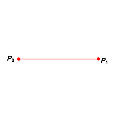
Figure 2: The initial line segment.

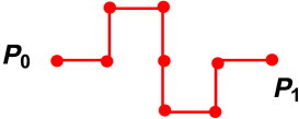
Figure 3: The graph obtained at the first iteration.

2 Framework of the study

In the sequel, we place ourselves in the Euclidean plane of dimension 2, referred to a direct orthonormal frame. The usual Cartesian coordinates are $(x,y)$.

Notation.

Let us denote by $P_{0}$ and  $P_{1}$ the points:

$$P_{0}=(0,0)\quad,\quad P_{1}=(1,0)$$

Notation.

Let us denote by $\theta\,\in\,]0,2\,\pi[$, $k>0$, $T_{1}$, and $T_{2}$ real numbers. Let us consider the rotation matrix:

$${\cal R}_{O,\theta}=\left(\begin{matrix}\cos\theta&-\sin\theta\\ \sin\theta&\cos\theta\\ \end{matrix}\right)$$

We introduce the iterated function system of the family of maps from ${\mathbb{R}}^{2}$ to ${\mathbb{R}}^{2}$:

$$\left\{f_{1},...,f_{8}\right\}$$

where, for any integer $i$ belonging to $\left\{1,...,8\right\}$, and any $X\,\in{\mathbb{R}}^{2}$:

$$f_{i}(X)=k\,{\cal R}_{O,\theta}X+\left(\begin{matrix}T_{1}\\ T_{2}\\ \end{matrix}\right)$$

Remark 2.1.

If $0<k<1$, the family $\left\{f_{1},...,f_{8}\right\}$ is a family of contractions from ${\mathbb{R}}^{2}$ to ${\mathbb{R}}^{2}$, the ratio of which is $k$.

Property 2.1.

According to [Hut81], there exists a unique subset $\mathfrak{MC}\subset{\mathbb{R}}^{2}$ such that:

$$\mathfrak{MC}=\underset{i=1}{\overset{8}{\bigcup}}\,f_{i}(\mathfrak{MC})$$

which will be called the Minkowski Curve.

One may note that this curve is not strictly self-similar in the sense defined by B. Mandelbrot [Man77], [Hut81]:

$$\exists\,(i,j)\,\in\leavevmode\nobreak\ \left\{f_{1},...,f_{8}\right\}^{2},\,i\neq j\,:\quad f_{i}(\mathfrak{MC})\cap f_{j}(\mathfrak{MC})\neq\emptyset$$

Definition 2.1.

We will denote by $V_{0}$ the ordered set, of the points:

$$\left\{P_{0},P_{1}\right\}$$

The set of points $V_{0}$, where, for any $i$ of $\left\{0,1\right\}$, the point $P_{0}$ is linked to the point $P_{1}$, constitutes an oriented graph, that we will denote by ${\mathfrak{MC}}_{0}$. $V_{0}$ is called the set of vertices of the graph ${\mathfrak{MC}}_{0}$.

For any strictly positive integer $m$, we set:

$$V_{m}=\underset{i=1}{\overset{8}{\bigcup}}\,f_{i}\left(V_{m-1}\right)$$

The set of points $V_{m}$, where the points of an $m$-cell are linked in the same way as ${\mathfrak{MC}}_{0}$, is an oriented graph, which we will denote by ${\mathfrak{MC}}_{m}$. $V_{m}$ is called the set of vertices of the graph ${\mathfrak{MC}}_{m}$. We will denote, in the following, by ${\cal N}_{m}$ the number of vertices of the graph ${\mathfrak{MC}}_{m}$.

Notation.

We introduce the following similarities, from ${\mathbb{R}}^{2}$ to ${\mathbb{R}}^{2}$, such that, for any $X\,\in\,{\mathbb{R}}^{2}$:

$$f_{1}(X)=\displaystyle\frac{1}{4}\,\left({\cal R}_{O,0}\,X+\left(\begin{matrix}0\\ 0\\ \end{matrix}\right)\right)\quad,\quad f_{2}(X)=\displaystyle\frac{1}{4}\,\left({\cal R}_{O,\frac{\pi}{2}}\,X+\left(\begin{matrix}1\\ 0\\ \end{matrix}\right)\right)\quad,\quad f_{3}(X)=\displaystyle\frac{1}{4}\,\left({\cal R}_{O,0}\,X+\left(\begin{matrix}1\\ 1\\ \end{matrix}\right)\right)$$

$$f_{4}(X)=\displaystyle\frac{1}{4}\,\left({\cal R}_{O,\frac{3\,\pi}{2}}\,X+\left(\begin{matrix}2\\ 1\\ \end{matrix}\right)\right)\quad,\quad f_{5}(X)=\displaystyle\frac{1}{4}\left({\cal R}_{O,\frac{3\,\pi}{2}}\,X+\left(\begin{matrix}2\\ 0\\ \end{matrix}\right)\right)\quad,\quad f_{6}(X)=\displaystyle\frac{1}{4}\,\left({\cal R}_{O,0}\,X+\left(\begin{matrix}2\\ -1\\ \end{matrix}\right)\right)$$

$$f_{7}(X)=\displaystyle\frac{1}{4}\,\left({\cal R}_{O,\frac{\pi}{2}}\,X+\left(\begin{matrix}3\\ -1\\ \end{matrix}\right)\right)\quad,\quad f_{8}(X)=\displaystyle\frac{1}{4}\,\left({\cal R}_{O,0}\,X+\left(\begin{matrix}3\\ 0\\ \end{matrix}\right)\right)\\$$

Property 2.2.

The set of vertices $\left(V_{m}\right)_{m\in{\mathbb{N}}}$ is dense in ${\mathfrak{MC}}$.

Proposition 2.3.

Given a natural integer $m$, we will denote by $\mathcal{N}_{m}$ the number of vertices of the graph ${\mathfrak{MC}}_{m}$. One has:

$$\mathcal{N}_{0}=2$$

and, for any strictly positive integer $m$:

$$\mathcal{N}_{m}=8\times\mathcal{N}_{m-1}-7$$

Proof.

The proposition results from the fact that, for any strictly positive integer $m$, each graph ${\mathfrak{MC}}_{m}$ is the union of eight copies of ${\mathfrak{MC}}_{m-1}$: every copy shares one vertex with its predecessor.
∎

Definition 2.2.

Consecutive vertices of ${\mathfrak{MC}}$

Let us set: $P_{2}=P_{0}$. Two points $X$ and $Y$ of ${\mathfrak{MC}}$ will be called consecutive vertices of ${\mathfrak{MC}}$ if there exists a natural integer $m$, and an integer $j$ of $\left\{0,1\right\}$, such that:

$$X=\left(f_{i_{1}}\circ\ldots\circ f_{i_{m}}\right)(P_{j})\quad\text{and}\quad Y=\left(f_{i_{1}}\circ\ldots\circ f_{i_{m}}\right)(P_{j+1})\qquad\left(i_{1},\ldots,i_{m}\right)\,\in\,\left\{1,\dots,8\right\}^{m}$$

Definition 2.3.

Edge relation, on the graph $\mathfrak{MC}$

Given a natural integer $m$, two points $X$ and $Y$ of ${\mathfrak{MC}}_{m}$ will be called adjacent if and only if $X$ and $Y$ are two consecutive vertices of ${\mathfrak{MC}}_{m}$. We will write:

$$X\underset{m}{\sim}Y$$

Definition 2.4.

For any positive integer $m$, the ${\cal N}_{m}$ consecutive vertices of the graph ${\mathfrak{MC}}_{m}$ are, also, the vertices of two triangles ${\cal T}_{m,left}$, ${\cal T}_{m,right}$, and $2\times 8^{m-1}$ squares ${\cal Q}_{m,j}$, $1\leqslant j\leqslant 2\times 8^{m-1}$. For any integer $j$ such that $1\leqslant j\leqslant 2\times 8^{m-1}$, one obtains each square by linking the point number $j$ to the point number $j+1$ if $j=i\,\text{mod }9$, $1\leqslant i\leqslant 3$, and the point number $j$ to the point number $j-3$ if $j=4\,\text{mod }9$, and the triangles by linking the point number $j$ to the point number $j+1$ and $j+2$ if $j=0\,\text{mod }9$. One has to consider those polygons as semi-closed ones, since, for any of those $4-$gons, the starting vertex, i.e. the point number $j$, is not connected, on the graph ${\mathfrak{MC}}_{m}$, to the extreme one, i.e. the point number $j-3$. In the same way, the extreme vertices of the two triangles ${\cal T}_{m,left}$, ${\cal T}_{m,right}$, are not connected, on the graph ${\mathfrak{MC}}_{m}$.
The reunion of those triangles and squares generate a Borel set of ${\mathbb{R}}^{2}$.

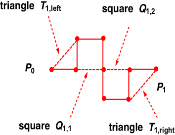
Figure 4: The triangles ${\cal T}_{1,left}$, ${\cal T}_{1,right}$, and the squares ${\cal Q}_{1,1}$, ${\cal Q}_{1,2}$.

Definition 2.5.

Quasi-quadrilateral domain delimited by the graph ${\mathfrak{MC}}_{m}$, $m\,\in\,{\mathbb{N}}$

For any natural integer $m$, we will call quasi-quadrilateral domain delimited by ${\mathfrak{MC}}_{m}$, and denote by ${\cal D}\left({{\mathfrak{MC}}_{m}}\right)$, the reunion of the triangles ${\cal T}_{m,j}$, and the squares ${\cal Q}_{m,j}$.

Definition 2.6.

Quasi-quadrilateral domain delimited by the Minkowski Curve ${\mathfrak{MC}}$

We will call quasi-quadrilateral domain delimited by ${\mathfrak{MC}}$, and denote by ${\cal D}\left({\mathfrak{MC}}\right)$, the limit:

$${\cal D}\left({\mathfrak{MC}}\right)=\displaystyle\lim_{n\to+\infty}{\cal D}\left({\mathfrak{MC}}_{m}\right)$$

which has to be understood in the following way: given a continuous function $u$ on the curve $\mathfrak{MC}$, and a measure with full support $\mu$ on ${\mathbb{R}}^{2}$, then:

$$\int_{{\cal D}\left({\mathfrak{MC}}\right)}\!u\,d\mu=\displaystyle\lim_{m\to+\infty}\left\{\displaystyle\frac{1}{3}\displaystyle\sum_{X\,\text{vertex of }{\cal T}_{m,left}}\!\!\!\!\!\!\!\!u\left(X\right)\,\mu\left({\cal T}_{m,left}\right)+\displaystyle\frac{1}{4}\displaystyle\sum_{j=1}^{2\times 8^{m-1}}\!\!\displaystyle\sum_{X\,\text{vertex of }{\cal Q}_{m,j}}\!\!\!\!\!\!\!\!u\left(X\right)\,\mu\left({\cal Q}_{m,j}\right)+\displaystyle\frac{1}{3}\displaystyle\sum_{X\,\text{vertex of }{\cal T}_{m,right}}\!\!\!\!\!\!\!\!u\left(X\right)\,\mu\left({\cal T}_{m,right}\right)\right\}$$

Remark 2.2.

One may wonder why consider such a quasi-quadrilateral domain, whereas we presently deal with a curve ? If it seemed, to us, the most natural way to perform integration on our fractal curve, there are, also, additionnal reasons. Part of an explanation can be found in the paper of U. Mosco [Mos02], where the author suggests, in the case of the Sierpiński curve, to "fill each small simplex (…) not only with its edges, but with the whole portion of the limit curve which it encompasses." It is also natural, in so far as it enables one to take into account the self-similar patterns that appear thanks to the curve, patterns, the measure of which plays the part of a pound. This joins the seminal work of J. Harrison et al. [HN91],  [HN92],  [Har93].

Definition 2.7.

Word, on the Minkowski curve  ${\mathfrak{MC}}$

Let $m$ be a strictly positive integer. We will call number-letter any integer ${\cal W}_{i}$ of $\left\{1,\dots,8\right\}$, and word of length $|{\cal W}|=m$, on the graph $\mathfrak{MC}$, any set of number-letters of the form:

$${\cal W}=\left({\cal W}_{1},\ldots,{\cal W}_{m}\right)$$

We will write:

$$f_{\cal W}=f_{{\cal W}_{1}}\circ\ldots\circ f_{{\cal W}_{m}}$$

Proposition 2.4.

Adresses, on the the Minkowski Curve

• Every $P_{i}$, $i\,\in\,\{0,1\}$, has exactly one neighbor.

• Given a strictly positive integer $m$, every $X\,\in\,V_{m}\setminus V_{0}$ has exactly two neighbors and two addresses

  $$X=f_{\left({\cal W}_{1},\ldots,{\cal W}_{m}\right)}(P_{0})=f_{\left({\cal W^{\prime}}_{1},\ldots,{\cal W^{\prime}}_{m}\right)}(P_{1})$$

  where ${\cal W}=\left({\cal W}_{1},\ldots,{\cal W}_{m}\right)$ and ${\cal W^{\prime}}=\left({\cal W^{\prime}}_{1},\ldots,{\cal W^{\prime}}_{m}\right)$ denote two appropriate words of length $m$, on the graph ${\mathfrak{MC}}_{m}$ (see [Str06]).

Proposition 2.5.

Let us set:

$${V_{\star}=\underset{{m\in{\mathbb{N}}}}{\bigcup}\,V_{m}}$$

The set $V_{\star}$ is dense in $\mathfrak{MC}$.

3 Energy forms, on the Minkowski Curve

3.1 Dirichlet forms

Definition 3.1.

Dirichlet form, on a finite set (We refer to [Kig03])

Let $V$ denote a finite set $V$, equipped with the usual inner product which, to any pair $(u,v)$ of functions defined on $V$, associates:

$$(u,v)=\displaystyle\sum_{P\in V}u(P)\,v(P)$$

A Dirichlet form on $V$ is a symmetric bilinear form ${\cal E}$, such that:

1. For any real valued function $u$ defined on $V$: ${\cal E}(u,u)\geqslant 0$.

2. ${\cal{E}}(u,u)=0$ if and only if $u$ is constant on $V$.

3. For any real-valued function $u$ defined on $V$, if:

   $$u_{\star}=\min\,(\max(u,0),1)$$

   i.e. :

   $$\forall\,p\,\in\,V\,:\quad u_{\star}(p)=\left\{\begin{array}[]{ccc}1&\text{if}&u(p)\geqslant 1\\ u(p)&\text{si}&0<u(p)<1\\ 0&\text{if}&u(p)\leqslant 0\end{array}\right.$$

   then: ${\cal{E}}(u_{\star},u_{\star})\leqslant{\cal{E}}(u,u)$ (Markov property).

Let us now consider the problem of energy forms on our curve. Such a problem was studied by U. Mosco [Mos02], who suggested to generalize Riemaniann models to fractals and relate the fractal analogous of gradient forms, i.e. the Dirichlet forms, to a metric that could reflect the fractal properties of the considered structure. The link is to be made by means of specific energy forms.

There are two major features that enable one to characterize fractal structures:

1. Their topology, i.e. their ramification.

2. Their geometry.
   

The topology can be taken into account by means of classical energy forms (we refer to [Kig89],  [Kig93], [Str99], [Str06]).
As for the geometry, again, things are not that simple to handle. U. Mosco introduces a strictly positive parameter, $\delta$, which is supposed to reflect the way ramification - or the iterative process that gives birth to the sequence of graphs that approximate the structure - affects the initial geometry of the structure. For instance, if $m$ is a natural integer, $X$ and $Y$ two points of the initial graph $V_{1}$, and $\cal M$ a word of length $m$, the Euclidean distance $d_{{\mathbb{R}}^{2}}(X,Y)$ between  $X$ and $Y$ is changed into the effective distance:

$$\left(d_{{\mathbb{R}}^{2}}(X,Y)\right)^{\delta}$$

This parameter $\delta$ appears to be the one that can be obtained when building the effective resistance metric of a fractal structure (see [Str06]), which is obtained by means of energy forms. To avoid turning into circles, this means:

1. either working, in a first time, with a value $\delta_{0}$ equal to one, and, then, adjusting it when building the effective resistance metric ;

2. using existing results, as done in [FL04].

One may note that in a very interesting and useful remark, U. Mosco puts the light on the relation that exists between the walk dimension $D_{W}$ of a self-similar set, and $\delta$:

$$D_{W}=2\,\delta$$

which will enable us to obtain the required value of the constant $\delta$.

Definition 3.2.

Walk dimension

Given a strictly positive integer $N$, the dimension related to a random walk on a self-similar set with respect to $N$ similarities, the ratio of which is equal to $k\,\in\,]0,1[$, is given by:

$$D_{W}=-\frac{\ln\mathbf{E}_{A}(\tau)}{\ln k}$$

where $\mathbf{E}_{A}(\tau)$ is the mean crossing time of a random walk starting from a vertex $A$ of the self-similar set.

Notation.

In the sequel, we will denote by $D_{W}\left(\mathfrak{MC}\right)$ the Walk dimension of the Minkowski Curve.

Remark 3.1.

Explicit computation of the Walk dimension of the Minkowski Curve

In the sequel, we follow the algorithm described in [FT13], which uses the theory of Markov chains (we refer to [KS83]).

To this purpose, we define $\mathbb{E}_{X}(\tau)$ to be the mean number of steps a simple random walk needs to reach a vertex ${B}\in V_{0}$ when starting at $X$. We consider the graph $\mathfrak{MI}_{1}$ and denote by $X_{i}$ for $i\in\{1,...,7\}$ the set of vertices of $V_{1}\setminus V_{0}$:

Figure 5: The graph $\mathfrak{MI}_{1}$

First, one has to introduce the adjacency matrix of the graph $\mathfrak{MI}_{1}$:

$$A_{\mathfrak{MI}_{1}}=\left(\begin{array}[]{ccccccccc}0&1&0&0&0&0&0&0&0\\ 1&0&1&0&0&0&0&0&0\\ 0&1&0&1&0&0&0&0&0\\ 0&0&1&0&1&0&0&0&0\\ 0&0&0&1&0&1&0&0&0\\ 0&0&0&0&1&0&1&0&0\\ 0&0&0&0&0&1&0&1&0\\ 0&0&0&0&0&0&1&0&1\\ 0&0&0&0&0&0&0&1&0\\ \end{array}\right)$$

One then build the related stochastic matrix:

$$A_{\mathfrak{MI}_{1}}^{stoch}=\left(\begin{array}[]{ccccccccc}0&1&0&0&0&0&0&0&0\\ \frac{1}{2}&0&\frac{1}{2}&0&0&0&0&0&0\\ 0&\frac{1}{2}&0&\frac{1}{2}&0&0&0&0&0\\ 0&0&\frac{1}{2}&0&\frac{1}{2}&0&0&0&0\\ 0&0&0&\frac{1}{2}&0&\frac{1}{2}&0&0&0\\ 0&0&0&0&\frac{1}{2}&0&1&0&0\\ 0&0&0&0&0&\frac{1}{2}&0&\frac{1}{2}&0\\ 0&0&0&0&0&0&\frac{1}{2}&0&\frac{1}{2}\\ 0&0&0&0&0&0&0&1&0\\ \end{array}\right)$$

By suppressing the lines and columns associated to one may call "cemetary states" (i.e. the fixed points of the contractions), one obtains the matrix:

$$M_{\mathfrak{MI}_{1}}=\left(\begin{array}[]{ccccccccc}0&1&0&0&0&0&0&0\\ \frac{1}{2}&0&\frac{1}{2}&0&0&0&0&0\\ 0&\frac{1}{2}&0&\frac{1}{2}&0&0&0&0\\ 0&0&\frac{1}{2}&0&\frac{1}{2}&0&0&0\\ 0&0&0&\frac{1}{2}&0&\frac{1}{2}&0&0\\ 0&0&0&0&\frac{1}{2}&0&1&0\\ 0&0&0&0&0&\frac{1}{2}&0&\frac{1}{2}\\ 0&0&0&0&0&0&\frac{1}{2}&0\\ \end{array}\right)$$

Starting at $P_{0}$, one has:

$$\mathbb{E}_{P_{0}}(\tau)=\mathbf{E}_{X_{1}}(\tau)+1\quad,\quad\mathbb{E}_{P_{1}}(\tau)=0$$

$$\mathbb{E}_{X_{1}}(\tau)=\displaystyle\frac{1}{2}\,\left(\mathbb{E}_{P_{0}}+\mathbf{E}_{X_{2}}(\tau)\right)+1\quad,\quad\mathbb{E}_{X_{2}}(\tau)=\displaystyle\frac{1}{2}\,\left(\mathbb{E}_{X_{1}}+\mathbb{E}_{X_{3}}(\tau)\right)+1\quad,\quad\mathbb{E}_{X_{3}}(\tau)=\displaystyle\frac{1}{2}\,\left(\mathbb{E}_{X_{2}}+\mathbb{E}_{X_{4}}(\tau)\right)+1$$

$$\mathbb{E}_{X_{4}}(\tau)=\displaystyle\frac{1}{2}\,\left(\mathbb{E}_{X_{3}}+\mathbb{E}_{X_{5}}(\tau)\right)+1\quad,\quad\mathbb{E}_{X_{5}}(\tau)=\displaystyle\frac{1}{2}\,\left(\mathbb{E}_{X_{4}}+\mathbb{E}_{X_{6}}(\tau)\right)+1\quad,\quad\mathbb{E}_{X_{6}}(\tau)=\displaystyle\frac{1}{2}\,\left(\mathbb{E}_{X_{5}}+\mathbb{E}_{X_{7}}(\tau)\right)+1$$

$$\mathbb{E}_{X_{7}}(\tau)=\displaystyle\frac{1}{2}\,\left(\mathbb{E}_{P_{1}}+\mathbb{E}_{X_{6}}(\tau)\right)+1$$

Let us introduce the vector of expected crossing-times:

$$\mathbb{T}=\left(\begin{array}[]{c}\mathbb{E}_{P_{0}}(\tau)\\ \mathbb{E}_{X_{1}}(\tau)\\ \mathbb{E}_{X_{2}}(\tau)\\ \mathbb{E}_{X_{3}}(\tau)\\ \mathbb{E}_{X_{4}}(\tau)\\ \mathbb{E}_{X_{5}}(\tau)\\ \mathbb{E}_{X_{6}}(\tau)\\ \mathbb{E}_{X_{7}}(\tau)\\ \end{array}\right)$$

From the theory of Markov chains, we have :

$$\mathbb{T}=\left({\mathbb{E}}_{\mathfrak{MI}_{1}}-M_{\mathfrak{MI}_{1}}\right)^{-1}\mathbf{1}$$

where $\mathbf{1}:=(1,...,1)^{T}$. By solving the above system, one gets:

$$\mathbb{T}=\left(\begin{array}[]{c}64\\ 63\\ 60\\ 55\\ 48\\ 39\\ 28\\ 15\\ \end{array}\right)$$

which leads to:

$$\mathbb{E}_{P_{1}}(\tau)=\displaystyle 64$$

and:

$$D_{W}\left(\mathfrak{MC}\right)=\displaystyle\frac{\ln 64}{\ln 4}=3$$

one has thus:

$$\delta=\displaystyle\frac{D_{W}\left(\mathfrak{MC}\right)}{2}=\displaystyle\frac{3}{2}$$

Definition 3.3.

Energy, on the graph ${\mathfrak{MC}}_{m}$, $m\,\in\,{\mathbb{N}}$, of a pair of functions

Let $m$ be a natural integer, and $u$ and $v$ two real valued functions, defined on the set

$$V_{m}=\left\{X_{1}^{m},\ldots,X_{{\cal N}_{m}^{\cal S}}^{m}\right\}$$

of the ${\cal N}_{m}$ vertices of ${\mathfrak{MC}}_{m}$.

We introduce the energy, on the graph ${\mathfrak{MC}}_{m}$, of the pair of functions $(u,v)$, as:

$$\begin{array}[]{ccc}{\cal{E}}_{{\mathfrak{MC}}_{m}}(u,v)&=&\displaystyle\sum_{i=1}^{{\cal N}_{m}-1}\left(\displaystyle\frac{u\left(X_{i}^{m}\right)-u\left(X_{i+1}^{m}\right)}{d_{{\mathbb{R}}^{2}}^{\delta}(X,Y)}\right)\,\left(\displaystyle\frac{v\left(X_{i}^{m}\right)-v\left(X_{i+1}^{m}\right)}{d_{{\mathbb{R}}^{2}}^{\delta}(X,Y)}\right)\\ &=&\displaystyle\sum_{i=1}^{{\cal N}_{m}-1}4^{2\,m\,\delta}\,\left(u\left(X_{i}^{m}\right)-u\left(X_{i+1}^{m}\right)\right)\,\left(v\left(X_{i}^{m}\right)-v\left(X_{i+1}^{m}\right)\right)\\ \end{array}$$

For the sake of simplicity, we will write it under the form:

$${\cal{E}}_{{\mathfrak{MC}}_{m}}(u,v)=\displaystyle\sum_{X\underset{m}{\sim}Y}4^{2\,m\,\delta}\,\left(u(X)-u(Y)\right)\,\left(v(X)-v(Y)\right)$$

Proposition 3.1.

Harmonic extension of a function, on the Minkowski Curve - Ramification constant

For any integer $m>1$, if $u$ is a real-valued function defined on $V_{m-1}$, its harmonic extension, denoted by $\tilde{u}$, is obtained as the extension of $u$ to $V_{m}$ which minimizes the energy:

$${\cal{E}}_{{\mathfrak{MC}}_{m}}(\tilde{u},\tilde{u})=\displaystyle\sum_{X\underset{m}{\sim}Y}4^{2\,m\,\delta}\,(\tilde{u}(X)-\tilde{u}(Y))^{2}$$

The link between ${\cal{E}}_{{\mathfrak{MC}}_{m}}$ and ${\cal{E}}_{{\mathfrak{MC}}_{m-1}}$ is obtained through the introduction of two strictly positive constants $r_{m}$ and $r_{m-1}$ such that:

$$r_{m}\,\displaystyle\sum_{X\underset{m+1}{\sim}Y}4^{2\,(m+1)\,\delta}\,(\tilde{u}(X)-\tilde{u}(Y))^{2}=r_{m-1}\,4^{2\,(m-1)\,\delta}\,\sum_{X\underset{m-1}{\sim}Y}(u(X)-u(Y))^{2}$$

For the sake of simplicity, we will fix the value of the initial constant: $r_{0}=1$.

$$r=\displaystyle\frac{1}{r_{1}}$$

By induction, one gets:

$$r_{m}=r_{1}^{m}=r^{-m}$$

and:

$${\cal{E}}_{m}(u)=r^{-m}\,4^{2\,m\,\delta}\,\sum_{X\underset{m}{\sim}Y}(\tilde{u}(X)-\tilde{u}(Y))^{2}$$

Since the determination of the harmonic extension of a function appears to be a local problem, on the graph ${\mathfrak{MC}}_{m-1}$, which is linked to the graph ${\mathfrak{MC}}_{m}$ by a similar process as the one that links ${\mathfrak{MC}}_{1}$ to ${\mathfrak{MC}}_{0}$, one deduces, for any integer $m>1$:

$${\cal{E}}_{{\mathfrak{MC}}_{m}}(\tilde{u},\tilde{u})=r^{-m}\,4^{2\,m\,\delta}\,{\cal{E}}_{{\mathfrak{MC}}_{m-1}}(\tilde{u},\tilde{u})$$

If $v$ is a real-valued function, defined on $V_{m-1}$, of harmonic extension $\tilde{v}$, we will write:

$${\cal{E}}_{m}(u,v)=r^{-m}\,\displaystyle\sum_{X\underset{m}{\sim}Y}4^{2\,m\,\delta}\,(\tilde{u}(X)-\tilde{u}(Y))\,(\tilde{v}(X)-\tilde{v}(Y))=r^{-m}\,\displaystyle\sum_{X\underset{m}{\sim}Y}4^{3\,m}\,(\tilde{u}(X)-\tilde{u}(Y))\,(\tilde{v}(X)-\tilde{v}(Y))$$

The constant $r^{-1}$, which can be interpreted as a topological one, will be called ramification constant.
For further precision on the construction and existence of harmonic extensions, we refer to [Sab97].

Definition 3.4.

Energy scaling factor

By definition, the energy scaling factor is the strictly positive constant $\rho$ such that, for any integer $m>1$, and any real-valued function $u$ defined on $V_{m}$:

$${\cal{E}}_{{\mathfrak{MC}}_{m}}(u,u)=\rho\,{\cal{E}}_{{\mathfrak{MC}}_{m}}\left(u_{\mid V_{m-1}},u_{\mid V_{m-1}}\right)$$

Proposition 3.2.

The energy scaling factor $\rho$ is linked to the topology and the geometry of the fractal curve by means of the relation:

$$\rho=\displaystyle\frac{4^{2\,\delta}}{8}=8$$

One may note that a more general calculation of the energy scaling factor can be found in the work by R. Capitanelli [Cap02].

3.2 Explicit computation of the ramification constant

3.2.1 Direct method

Let us denote by $u$ a real-valued, continuous function defined on $V_{0}=\{P_{0},P_{1}\}$, and by $\tilde{u}$ its harmonic extension to $V_{1}$. Let us set: $u(P_{0})=A$, $u(P_{1})=B$. We recall that the energy on $V_{0}$ is given by :

$$E_{0}(u)=(A-B)^{2}$$

We will denote by $U_{1}$, $U_{2}$, $U_{3}$, $U_{4}$, $U_{5}$, $U_{6}$, $U_{7}$, $U_{16}$, the respective images, by $\tilde{u}$, of the vertices of $V_{1}\setminus V_{0}$.

One has then:

$$E_{1}(\tilde{u})=(A-U_{1})^{2}+(U_{1}-U_{2})^{2}+(U_{2}-U_{3})^{2}+(U_{3}-U_{4})^{2}+(U_{4}-U_{5})^{2}+(U_{5}-U_{6})^{2}+(U_{6}-U_{7})^{2}+(U_{7}-B)^{2}$$

The minimum of this quantity is such that:

$$\mathbf{U}=\mathbf{A}^{-1}\,\mathbf{b}$$

where the matrix $A$ is given by:

$$\mathbf{A}=\left(\begin{array}[]{ccccccc}2&-1&0&0&0&0&0\\ -1&2&-1&0&0&0&0\\ 0&-1&2&-1&0&0&0\\ 0&0&-1&2&-1&0&0\\ 0&0&0&-1&2&-1&0\\ 0&0&0&0&-1&2&-1\\ 0&0&0&0&0&-1&2\\ \end{array}\right)$$

the vectors $\mathbf{U}$ and $\mathbf{b}$ by:

$$\mathbf{U}=\begin{pmatrix}U_{1}\\ U_{2}\\ U_{3}\\ U_{4}\\ U_{5}\\ U_{6}\\ U_{7}\\ \end{pmatrix}\quad,\quad\mathbf{b}=\left(\begin{array}[]{c}A\\ 0\\ 0\\ 0\\ 0\\ 0\\ B\\ \end{array}\right)$$

One obtains:

$$\mathbf{U}=\left(\begin{array}[]{c}\frac{7A}{8}+\frac{B}{8}\\ \frac{3A}{4}+\frac{B}{4}\\ \frac{5A}{8}+\frac{3B}{8}\\ \frac{A}{2}+\frac{B}{2}\\ \frac{3A}{8}+\frac{5B}{8}\\ \frac{A}{4}+\frac{3B}{4}\\ \frac{A}{8}+\frac{7B}{8}\\ \end{array}\right)$$

By substituting these values in the expression of the energy expression, one obtains:

$$E_{1}(\tilde{u})=\displaystyle\frac{(A-B)^{2}}{8}=\displaystyle\frac{1}{8}\,E_{0}(u)$$

Thus:

$$r=\displaystyle\frac{1}{8}$$

3.2.2 A second method, using Einstein’s relation

Definition 3.5.

Hausdorff dimension of a self-similar set with respect to $N\,\in\,{\mathbb{N}}^{\star}$ similarities

Given a strictly positive integer $N$, the Hausdorff dimension of a self-similar set with respect to $N$ similarities, the ratio of which is equal to $k\,\in\,]0,1[$, is given by:

$$D_{H}=-\frac{\ln N}{\ln k}$$

Notation.

In the sequel, we will denote by

$$D_{H}\left(\mathfrak{MC}\right)=-\frac{\ln 8}{\ln k}$$

the Hausdorff dimension of the Minkowski Curve.

Definition 3.6.

Spectral dimension of a self-similar set with respect to $N\,\in\,{\mathbb{N}}^{\star}$ similarities

Given a strictly positive integer $N$, the spectral dimension of a self-similar set with respect to $N$ similarities, the energy scaling factor of which is equal to $\rho$, is given by:

$$D_{S}=\frac{2\,\ln N}{\ln(N\times\rho)}$$

Notation.

In the sequel, we will denote by

$$D_{S}\left(\mathfrak{MC}\right)=\frac{6\,\ln 2}{\ln(8\times\rho)}$$

the spectral dimension of the Minkowski Curve.

Theorem 3.3.

Einstein relation

Given a strictly positive integer $N$, and a self-similar set with respect to $N$ similarities, the ratio of which is equal to $k\,\in\,]0,1[$, one has the so-called Einstein relation between the walk dimension, the Hausdorff dimension, and the spectral dimension of the set:

$$D_{H}=\frac{D_{S}\,D_{W}}{2}$$

Property 3.4.

Given a strictly positive integer $N$, and a self-similar set with respect to $N$ similarities, the ratio of which is equal to $k\,\in\,]0,1[$, the energy scaling factor $\rho$, which solely depends on the topology, and, therefore, not of the value of the contraction ratio, is given by:

$$\rho=\frac{\mathbb{E}_{A}(T)}{N}$$

Figure 6: The graph $\mathfrak{MC}_{0}$

3.3 Specific Dirichlet and energy forms, for the Minkowski Curve

Definition 3.7.

Dirichlet form, for a pair of continuous functions defined on the Minkowski Curve $\mathfrak{MC}$

We define the Dirichlet form $\cal{E}$ which, to any pair of real-valued, continuous functions $(u,v)$ defined on $\mathfrak{MC}$, associates, subject to its existence:

$${\cal{E}}(u,v)=\displaystyle\lim_{m\to+\infty}{\cal{E}}_{m}\left(u_{\mid V_{m}},v_{\mid V_{m}}\right)=\displaystyle\lim_{m\to+\infty}\displaystyle\sum_{X\underset{m}{\sim}Y}r^{-m}\,4^{2\,m\,\delta}\,\left(u_{\mid V_{m}}(X)-u_{\mid V_{m}}(Y)\right)\,\left(v_{\mid V_{m}}(X)-v_{\mid V_{m}}(Y)\right)$$

Definition 3.8.

Normalized energy, for a continuous function $u$, defined on $\mathfrak{MC}$
Taking into account that the sequence $\left(\mathcal{E}_{m}\left(u_{\mid V_{m}}\right)\right)_{m\in{\mathbb{N}}}$ is defined on

$${V_{\star}=\underset{{i\in{\mathbb{N}}}}{\bigcup}\,V_{i}}$$

one defines the normalized energy, for a continuous function $u$, defined on $\mathfrak{MC}$, by:

$$\mathcal{E}(u)=\underset{m\rightarrow+\infty}{\lim}\mathcal{E}_{m}\left(u_{\mid V_{m}}\right)$$

Property 3.5.

The Dirichlet form $\cal{E}$ which, to any pair of real-valued, continuous functions defined on $\mathfrak{MC}$, associates:

$${\cal{E}}(u,v)=\displaystyle\lim_{m\to+\infty}{\cal{E}}_{m}\left(u_{\mid V_{m}},v_{\mid V_{m}}\right)=\displaystyle\lim_{m\to+\infty}\displaystyle\sum_{X\underset{m}{\sim}Y}r^{-m}\,4^{2\,m\,\delta}\,\,\left(u_{\mid V_{m}}(X)-u_{\mid V_{m}}(Y)\right)\,\left(v_{\mid V_{m}}(X)-v_{\mid V_{m}}(Y)\right)$$

satisfies the self-similarity relation:

$${\cal{E}}(u,v)=r^{-1}\,4^{2\,\delta}\,\displaystyle\sum_{i=1}^{8}{\cal{E}}\left(u\circ f_{i},v\circ f_{i}\right)$$

Proof.

$$\begin{array}[]{ccc}\displaystyle\sum_{i=1}^{8}{\cal{E}}\left(u\circ f_{i},v\circ f_{i}\right)&=&\displaystyle\lim_{m\to+\infty}\displaystyle\sum_{i=1}^{8}{\cal{E}}_{m}\left(u_{\mid V_{m}}\circ f_{i},v_{\mid V_{m}}\circ f_{i}\right)\\ &=&\displaystyle\lim_{m\to+\infty}\displaystyle\sum_{X\underset{m}{\sim}Y}r^{-m}\,4^{2\,m\,\delta}\,\displaystyle\sum_{i=1}^{8}\left(u_{\mid V_{m}}\left(f_{i}(X)\right)-u_{\mid V_{m}}\left(f_{i}(Y)\right)\right)\,\left(v_{\mid V_{m}}\left(f_{i}(X)\right)-v_{\mid V_{m}}\left(f_{i}(Y)\right)\right)\\ &=&\displaystyle\lim_{m\to+\infty}\displaystyle\sum_{X\underset{m+1}{\sim}Y}r^{-m}\,4^{2\,m\,\delta}\,\displaystyle\sum_{i=1}^{8}\left(u_{\mid V_{m+1}}(X)-u_{\mid V_{m+1}}(Y)\right)\,\left(v_{\mid V_{m+1}}(X)-v_{\mid V_{m+1}}(Y)\right)\\ &=&\displaystyle\lim_{m\to+\infty}r\,4^{-2\,\delta}\,{\cal{E}}_{m+1}\left(u_{\mid V_{m+1}},v_{\mid V_{m+1}}\right)\\ &=&r\,4^{-2\,\delta}\,{\cal{E}}(u,v)\\ \end{array}$$

∎

Notation.

We will denote by $\text{dom}\,{\cal E}$ the subspace of continuous functions defined on $\mathfrak{MC}$, such that:

$$\mathcal{E}(u)<+\infty$$

Notation.

We will denote by $\text{dom}_{0}\,{\cal E}$ the subspace of continuous functions defined on $\mathfrak{MC}$, which take the value $0$ on $V_{0}$, such that:

$$\mathcal{E}(u)<+\infty$$

Proposition 3.6.

The space $\text{dom}\mathcal{E}$, modulo the space of constant function on $\mathfrak{MC}$, is a Hilbert space.

4 Laplacian, on the Minkowski Curve

Definition 4.1.

Self-similar measure, on the domain delimited by the Minkowski Curve

A measure $\mu$ on ${\mathbb{R}}^{2}$ will be said to be self-similar domain delimited by the Minkowski Curve, if there exists a family of strictly positive pounds $\left(\mu_{i}\right)_{1\leqslant i\leqslant 8}$ such that:

$$\mu=\displaystyle\sum_{i=1}^{8}\mu_{i}\,\mu\circ f_{i}^{-1}\quad,\quad\displaystyle\sum_{i=1}^{8}\mu_{i}=1$$

For further precisions on self-similar measures, we refer to the works of J. E. Hutchinson (see [Hut81]).

Property 4.1.

Building of a self-similar measure, for the Minkowski Curve

The Dirichlet forms mentioned in the above require a positive Radon measure with full support.

Let us set for any integer $i$ belonging to $\left\{1,\ldots,8\right\}$:

$$\mu_{i}=R^{D_{H}\left(\mathfrak{MC}\right)}=\displaystyle\frac{1}{8}$$

This enables one to define a self-similar measure $\mu$ on $\mathfrak{MC}$ as:

$$\mu=\displaystyle\frac{1}{8}\,\sum_{i=1}^{8}\mu\circ f_{i}$$

Definition 4.2.

Laplacian of order $m\,\in\,{\mathbb{N}}^{\star}$

For any strictly positive integer $m$, and any real-valued function $u$, defined on the set $V_{m}$ of the vertices of the graph ${\mathfrak{MC}}_{m}$, we introduce the Laplacian of order $m$, $\Delta_{m}(u)$, by:

$$\Delta_{m}u(X)=\displaystyle\sum_{Y\in V_{m},\,Y\underset{m}{\sim}X}\left(u(Y)-u(X)\right)\quad\forall\,X\,\in\,V_{m}\setminus V_{0}$$

Definition 4.3.

Harmonic function of order $m\,\in\,{\mathbb{N}}^{\star}$

Let $m$ be a strictly positive integer. A real-valued function $u$,defined on the set $V_{m}$ of the vertices of the graph ${\mathfrak{MC}}_{m}$, will be said to be harmonic of order $m$ if its Laplacian of order $m$ is null:

$$\Delta_{m}u(X)=0\quad\forall\,X\,\in\,V_{m}\setminus V_{0}$$

Definition 4.4.

Piecewise harmonic function of order $m\,\in\,{\mathbb{N}}^{\star}$

Given a strictly positive integer $m$, a real valued function $u$, defined on the set of vertices of $\mathfrak{MC}$, is said to be piecewise harmonic function of order $m$ if, for any word ${\cal W}$ of length $m$, $u\circ f_{\cal W}$ is harmonic of order $m$.

Definition 4.5.

Existence domain of the Laplacian, for a continuous function on $\mathfrak{MC}$ (see [BD85])

We will denote by $\text{dom}\,\Delta$ the existence domain of the Laplacian, on the graph ${\mathfrak{MC}}$, as the set of functions $u$ of $\text{dom}\,\mathcal{E}$ such that there exists a continuous function on $\mathfrak{MC}$, denoted $\Delta\,u$, that we will call Laplacian of $u$, such that :

$$\mathcal{E}(u,v)=-\displaystyle\int_{{\cal D}\left({\mathfrak{MC}}\right)}v\,\Delta u\,d\mu\quad\text{for any }v\,\in\,\text{dom}_{0}\,\mathcal{E}$$

Definition 4.6.

Harmonic function

A function $u$ belonging to $\text{dom}\,\Delta$ will be said to be harmonic if its Laplacian is equal to zero.

Notation.

In the following, we will denote by ${\cal H}_{0}\subset\text{dom}\,\Delta$ the space of harmonic functions, i.e. the space of functions $u\,\in\,\ \text{dom}\,\Delta$ such that:

$$\Delta\,u=0$$

Given a natural integer $m$, we will denote by ${\cal S}\left({\cal H}_{0},V_{m}\right)$ the space, of dimension $8^{m}$, of spline functions " of level $m$",  $u$, defined on ${\mathfrak{MC}}$, continuous, such that, for any word $\cal W$ of length $m$, $u\circ T_{\cal W}$ is harmonic, i.e.:

$$\Delta_{m}\,\left(u\circ T_{\cal W}\right)=0$$

Property 4.2.

For any natural integer $m$:

$${\cal S}\left({\cal H}_{0},V_{m}\right)\subset\text{dom }{\cal E}$$

Property 4.3.

Let $m$ be a strictly positive integer, $X\,\notin\,V_{0}$ a vertex of the graph $\mathfrak{MC}$, and $\psi_{X}^{m}\,\in\,{\cal S}\left({\cal H}_{0},V_{m}\right)$ a spline function such that:

$$\psi_{X}^{m}(Y)=\left\{\begin{array}[]{ccc}\delta_{XY}&\forall&Y\,\in\,V_{m}\\ 0&\forall&Y\,\notin\,V_{m}\end{array}\right.\quad,\quad\text{where}\quad\delta_{XY}=\left\{\begin{array}[]{ccc}1&\text{if}&X=Y\\ 0&\text{else}&\end{array}\right.$$

Then, since $X\,\notin\,V_{0}$: $\psi_{X}^{m}\,\in\,\text{dom}_{0}\,\mathcal{E}$.

For any function $u$ of $\text{dom}\,\mathcal{E}$, such that its Laplacian exists, definition (4.5) applied to $\psi_{X}^{m}$ leads to:

$$\mathcal{E}(u,\psi_{X}^{m})=\mathcal{E}_{m}(u,\psi_{X}^{m})=-r^{-m}\,\Delta_{m}u(X)=-\displaystyle\int_{{\cal D}\left({\mathfrak{MC}}\right)}\psi_{X}^{m}\,\Delta u\,d\mu\approx-\Delta u(X)\,\displaystyle\int_{{\cal D}\left({\mathfrak{MC}}\right)}\psi_{X}^{m}\,d\mu$$

since $\Delta u$ is continuous on ${\mathfrak{MC}}$, and the support of the spline function $\psi_{X}^{m}$ is close to $X$:

$$\int_{{\cal D}\left({\mathfrak{MC}}\right)}\psi_{X}^{m}\,\Delta u\,d\mu\approx-\Delta u(X)\,\displaystyle\int_{{\cal D}\left({\mathfrak{MC}}\right)}\psi_{X}^{m}\,d\mu$$

By passing through the limit when the integer $m$ tends towards infinity, one gets:

$$\lim_{m\to+\infty}\displaystyle\int_{{\cal D}\left({\mathfrak{MC}}\right)}\psi_{X}^{m}\,\Delta_{m}u\,d\mu=\Delta u(X)\,\displaystyle\lim_{m\to+\infty}\displaystyle\int_{{\cal D}\left({\mathfrak{MC}}\right)}\psi_{X}^{m}\,d\mu$$

i.e.:

$$\Delta u(X)=\displaystyle\lim_{m\to+\infty}r^{-m}\,4^{2\,m\,\delta}\,\left(\displaystyle\int_{{\cal D}\left({\mathfrak{MC}}\right)}\psi_{X}^{m}\,d\mu\right)^{-1}\,\Delta_{m}u(X)\,$$

Remark 4.1.

As it is explained in [Str06], one has just to reason by analogy with the dimension 1, more particulary, the unit interval $I=[0,1]$, of extremities $X_{0}=(0,0)$, and $X_{1}=(1,0)$. The functions $\psi_{X_{1}}$ and $\psi_{X_{2}}$ such that, for any $Y$ of ${\mathbb{R}}^{2}$ :

$$\psi_{X_{1}}(Y)=\delta_{X_{1}Y}\quad,\quad\psi_{X_{2}}(Y)=\delta_{X_{2}Y}$$

are, in the most simple way, tent functions. For the standard measure, one gets values that do not depend on $X_{1}$, or $X_{2}$ (one could, also, choose to fix $X_{1}$ and $X_{2}$ in the interior of $I$) :

$$\int_{I}\psi_{X_{1}}\,d\mu=\displaystyle\int_{I}\psi_{X_{2}}\,d\mu=\displaystyle\frac{1}{2}$$

(which corresponds to the surfaces of the two tent triangles.)

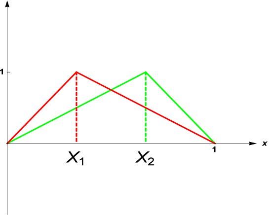
Figure 7: The graphs of the spline functions $\psi_{X_{1}}$ and $\psi_{X_{2}}$.

In our case, we have to build the pendant, we no longer reason on the unit interval, but on our triangular or square cells.

Given a natural integer $m$, and a point $X\,\in\,V_{m}$, the spline function $\psi_{X}^{m}$ is supported by two $m$-cells. It is such that, for every $m$-line cell $f_{\mathcal{W}}\left(\mathfrak{MC}\right)$ the vertices of which are $X$, $Y\neq X$ :

$$\psi_{X}^{m}+\psi_{Y}^{m}=1$$

Thus:

$$\int_{f_{\mathcal{W}}\left(\mathfrak{MC}\right)}\left(\psi_{X}^{m}+\psi_{Y}^{m}\right)\,d\mu=\mu(f_{\mathcal{W}}\left(\mathfrak{MC}\right))=\displaystyle\frac{1}{8^{m}}$$

By symmetry, all three summands have the same integral. This yields:

$${\int_{f_{\mathcal{W}}\left(\mathfrak{MC}\right)}\psi_{X}^{m}d\mu=\frac{1}{2\times 8^{m}}}$$

Taking into account the contributions of the remaining $m$-square cells, one has:

$${\int_{\mathfrak{MC}}\psi_{X}^{m}d\mu=\frac{1}{8^{m}}}$$

which leads to:

$$\left(\int_{\mathfrak{MC}}\psi_{X}^{m}\,d\mu\right)^{-1}=\displaystyle 8^{m}$$

Since:

$${r^{-m}=8^{m}}$$

this enables us to obtain the point-wise formula, for $u\,\in\,\text{dom}\,\Delta$:

$$\forall\,X\,\in\,{\mathfrak{MC}}\,:\quad\Delta_{\mu}u(X)=\displaystyle\lim_{m\rightarrow+\infty}64^{m}\,\Delta_{m}u(X)$$

Theorem 4.4.

Let $u$ be in $\text{dom}\,\Delta$. Then, the sequence of functions $\left(f_{m}\right)_{m\in{\mathbb{N}}}$ such that, for any natural integer $m$, and any $X$ of $V_{\star}\setminus V_{0}$ :

$$f_{m}(X)=r^{-m}\,4^{2\,m\,\delta}\,\left(\displaystyle\int_{{\cal D}\left({\mathfrak{MC}}\right)}\psi_{X}^{m}\,d\mu\right)^{-1}\,\Delta_{m}\,u(X)$$

converges uniformly towards $\Delta\,u$, and, reciprocally, if the sequence of functions $\left(f_{m}\right)_{m\in{\mathbb{N}}}$ converges uniformly towards a continuous function on $V_{\star}\setminus V_{0}$, then:

$$u\,\in\,\text{dom}\,\Delta$$

Proof.

Let $u$ be in $\text{dom}\,\Delta$. Then:

$$r^{-m}\,4^{2\,m\,\delta}\,\,\left(\displaystyle\int_{{\cal D}\left({\mathfrak{MC}}\right)}\psi_{X}^{m}\,d\mu\right)^{-1}\,\Delta_{m}\,u(X)=\displaystyle\frac{\displaystyle\int_{{\cal D}\left({\mathfrak{MC}}\right)}\Delta\,u\,\psi_{X}^{m}\,d\mu}{\displaystyle\int_{{\cal D}\left({\mathfrak{MC}}\right)}\psi_{X}^{m}\,d\mu}$$

Since $u$ belongs to $\text{dom}\,\Delta$, its Laplacian $\Delta\,u$ exists, and is continuous on the graph ${\mathfrak{MC}}$. The uniform convergence of the sequence $\left(f_{m}\right)_{m\in{\mathbb{N}}}$ follows.

Reciprocally, if the sequence of functions $\left(f_{m}\right)_{m\in{\mathbb{N}}}$ converges uniformly towards a continuous function on $V_{\star}\setminus V_{0}$, the, for any natural integer $m$, and any $v$ belonging to $\text{dom}_{0}\,{\cal E}$:

$$\begin{array}[]{ccc}{\cal{E}}_{m}(u,v)&=&\displaystyle\sum_{(X,Y)\,\in\,V_{m}^{2},\,X\underset{m}{\sim}Y}r^{-m}\,4^{2\,m\,\delta}\,\,\left(u_{\mid V_{m}}(X)-u_{\mid V_{m}}(Y)\right)\,\left(v_{\mid V_{m}}(X)-v_{\mid V_{m}}(Y)\right)\\ &=&\displaystyle\sum_{(X,Y)\,\in\,V_{m}^{2},\,X\underset{m}{\sim}Y}r^{-m}\,4^{2\,m\,\delta}\,\,\left(u_{\mid V_{m}}(Y)-u_{\mid V_{m}}(X)\right)\,\left(v_{\mid V_{m}}(Y)-v_{\mid V_{m}}(X)\right)\\ &=&-\displaystyle\sum_{X\,\in\,V_{m}\setminus V_{0}}r^{-m}\,4^{2\,m\,\delta}\,\,\sum_{Y\,\in\,V_{m},\,Y\underset{m}{\sim}X}v_{\mid V_{m}}(X)\,\left(u_{\mid V_{m}}(Y)-u_{\mid V_{m}}(X)\right)\\ &&-\displaystyle\sum_{X\,\in\,V_{0}}r^{-m}\,4^{2\,m\,\delta}\,\sum_{Y\,\in\,V_{m},\,Y\underset{m}{\sim}X}v_{\mid V_{m}}(X)\,\left(u_{\mid V_{m}}(Y)-u_{\mid V_{m}}(X)\right)\\ &=&-\displaystyle\sum_{X\,\in\,V_{m}\setminus V_{0}}r^{-m}\,4^{2\,m\,\delta}\,\,v(X)\,\Delta_{m}\,u(X)\\ &=&-\displaystyle\sum_{X\,\in\,V_{m}\setminus V_{0}}v(X)\,\left(\displaystyle\int_{{\cal D}\left({\mathfrak{MC}}\right)}\psi_{X}^{m}\,d\mu\right)\,r^{-m}\,4^{2\,m\,\delta}\,\left(\displaystyle\int_{{\cal D}\left({\mathfrak{MC}}\right)}\psi_{X}^{m}\,d\mu\right)^{-1}\,\Delta_{m}\,u(X)\\ \end{array}$$

Let us note that any $X$ of $V_{m}\setminus V_{0}$ admits exactly two adjacent vertices which belong to $V_{m}\setminus V_{0}$, which accounts for the fact that the sum

$$\sum_{X\,\in\,V_{m}\setminus V_{0}}r^{-m}\,4^{2\,m\,\delta}\,\sum_{Y\,\in\,V_{m}\setminus V_{0},\,Y\underset{m}{\sim}X}v(X)\,\left(u_{\mid V_{m}}(Y)-u_{\mid V_{m}}(X)\right)$$

has the same number of terms as:

$$\sum_{(X,Y)\,\in\,(V_{m}\setminus V_{0})^{2},\,X\underset{m}{\sim}Y}r^{-m}\,8^{2\,m\,\delta}\,\left(u_{\mid V_{m}}(Y)-u_{\mid V_{m}}(X)\right)\,\left(v_{\mid V_{m}}(Y)-v_{\mid V_{m}}(X)\right)$$

For any natural integer $m$, we introduce the sequence of functions $\left(f_{m}\right)_{m\in{\mathbb{N}}}$ such that, for any $X$ of $V_{m}\setminus V_{0}$:

$$f_{m}(X)=r^{-m}\,4^{2\,m\,\delta}\,\left(\displaystyle\int_{{\cal D}\left({\mathfrak{MC}}\right)}\psi_{X}^{m}\,d\mu\right)^{-1}\,\Delta_{m}\,u(X)$$

The sequence $\left(f_{m}\right)_{m\in{\mathbb{N}}}$ converges uniformly towards $\Delta\,u$. Thus:

$$\begin{array}[]{ccc}{\cal{E}}_{m}(u,v)&=&-\displaystyle\int_{{\cal D}\left({\mathfrak{MC}}\right)}\left\{\displaystyle\sum_{X\,\in\,V_{m}\setminus V_{0}}v_{\mid V_{m}}(X)\,\Delta\,u_{\mid V_{m}}(X)\,\psi_{X}^{m}\right\}\,d\mu\end{array}$$

∎

5 Normal derivatives

Let us go back to the case of a function $u$ twice differentiable on $I=[0,1]$, that does not vanish in 0 and :

$$\int_{0}^{1}\left(\Delta u\right)(x)\,v(x)\,dx=-\displaystyle\int_{0}^{1}u^{\prime}(x)\,v^{\prime}(x)\,dx+u^{\prime}(1)\,v(1)-u^{\prime}(0)\,v(0)$$

The normal derivatives:

$$\partial_{n}u(1)=u^{\prime}(1)\quad\text{et}\quad\partial_{n}u(0)=u^{\prime}(0)$$

appear in a natural way. This leads to:

$$\int_{0}^{1}\left(\Delta u\right)(x)\,v(x)\,dx=-\displaystyle\int_{0}^{1}u^{\prime}(x)\,v^{\prime}(x)\,dx+\displaystyle\sum_{\partial\,[0,1]}v\,\partial_{n}\,u$$

One meets thus a particular case of the Gauss-Green formula, for an open set $\Omega$ of ${\mathbb{R}}^{d}$, $d\,\in\,{\mathbb{N}}^{\star}$:

$$\int_{\Omega}\nabla\,u\,\nabla\,v\,d\mu=-\displaystyle\int_{\Omega}\left(\Delta u\right)\,v\,d\mu+\displaystyle\int_{\partial\,\Omega}v\,\partial_{n}\,u\,d\sigma$$

where $\mu$ is a measure on $\Omega$, and where $d\sigma$ denotes the elementary surface on $\partial\,\Omega$.

In order to obtain an equivalent formulation in the case of the graph $\mathfrak{MC}$, one should have, for a pair of functions $(u,v)$ continuous on $\mathfrak{MC}$ such that $u$ has a normal derivative:

$${\cal E}(u,v)=-\displaystyle\int_{\Omega}\left(\Delta u\right)\,v\,d\mu+\displaystyle\sum_{V_{0}}v\,\partial_{n}\,u$$

For any natural integer $m$ :

$$\begin{array}[]{ccc}{\cal{E}}_{m}(u,v)\\ &=&\displaystyle\sum_{(X,Y)\,\in\,V_{m}^{2},\,X\underset{m}{\sim}Y}r^{-m}\,4^{2\,m\,\delta}\,\left(u_{\mid V_{m}}(Y)-u_{\mid V_{m}}(X)\right)\,\left(v_{\mid V_{m}}(Y)-v_{\mid V_{m}}(X)\right)\\ &=&-\displaystyle\sum_{X\,\in\,V_{m}\setminus V_{0}}r^{-m}\,8^{2\,m\,\delta}\,\sum_{Y\,\in\,V_{m},\,Y\underset{m}{\sim}X}v_{\mid V_{m}}(X)\,\left(u_{\mid V_{m}}(Y)-u_{\mid V_{m}}(X)\right)\\ &&-\displaystyle\sum_{X\,\in\,V_{0}}r^{-m}\,4^{2\,m\,\delta}\,\sum_{Y\,\in\,V_{m},\,Y\underset{m}{\sim}X}v_{\mid V_{m}}(X)\,\left(u_{\mid V_{m}}(Y)-u_{\mid V_{m}}(X)\right)\\ &=&-\displaystyle\sum_{X\,\in\,V_{m}\setminus V_{0}}v_{\mid V_{m}}(X)\,r^{-m}\,4^{2\,m\,\delta}\,\Delta_{m}\,u_{\mid V_{m}}(X)\\ &&+\displaystyle\sum_{X\,\in\,V_{0}}\sum_{Y\,\in\,V_{m},\,Y\underset{m}{\sim}X}r^{-m}\,8^{2\,m\,\delta}\,v_{\mid V_{m}}(X)\,\left(u_{\mid V_{m}}(X)-u_{\mid V_{m}}(Y)\right)\\ \end{array}$$

We thus come across an analogous formula of the Gauss-Green one, where the role of the normal derivative is played by:

$$\sum_{X\,\in\,V_{0}}r^{-m}\,4^{2\,m\,\delta}\,\sum_{Y\,\in\,V_{m},\,Y\underset{m}{\sim}X}\,\left(u_{\mid V_{m}}(X)-u_{\mid V_{m}}(Y)\right)$$

Definition 5.1.

For any $X$ of $V_{0}$, and any continuous function $u$ on $\mathfrak{MC}$, we will say that $u$ admits a normal derivative in $X$, denoted by $\partial_{n}\,u(X)$, if:

$$\lim_{m\to+\infty}r^{-m}\,4^{2\,m\,\delta}\,\sum_{Y\,\in\,V_{m},\,Y\underset{m}{\sim}X}\,\left(u_{\mid V_{m}}(X)-u_{\mid V_{m}}(Y)\right)<+\infty$$

We will set:

$$\partial_{n}\,u(X)=\displaystyle\lim_{m\to+\infty}r^{-m}\,4^{2\,m\,\delta}\,\sum_{Y\,\in\,V_{m},\,Y\underset{m}{\sim}X}\,\left(u_{\mid V_{m}}(X)-u_{\mid V_{m}}(Y)\right)<+\infty$$

Definition 5.2.

For any natural integer $m$, any $X$ of $V_{m}$, and any continuous function $u$ on $\mathfrak{MC}$, we will say that $u$ admits a normal derivative in $X$, denoted by $\partial_{n}\,u(X)$, if:

$$\lim_{k\to+\infty}r^{-k}\,4^{2\,k\,\delta}\,\sum_{Y\,\in\,V_{k},\,Y\underset{k}{\sim}X}\,\left(u_{\mid V_{k}}(X)-u_{\mid V_{k}}(Y)\right)<+\infty$$

We will set:

$$\partial_{n}\,u(X)=\displaystyle\lim_{k\to+\infty}r^{-k}\,4^{2\,k\,\delta}\,\sum_{Y\,\in\,V_{k},\,Y\underset{k}{\sim}X}\,\left(u_{\mid V_{k}}(X)-u_{\mid V_{k}}(Y)\right)<+\infty$$

Remark 5.1.

One can thus extend the definition of the normal derivative of $u$ to $\mathfrak{MC}$.

Theorem 5.1.

Let $u$ be in $\text{dom}\,\Delta$. The, for any $X$ of $\mathfrak{MC}$, $\partial_{n}\,u(X)$ exists. Moreover, for any $v$ of $\text{dom}\,\cal E$, et any natural integer $m$, the Gauss-Green formula writes:

$${\cal E}(u,v)=-\displaystyle\int_{{\cal D}\left({\mathfrak{MC}}\right)}\left(\Delta u\right)\,v\,d\mu+\displaystyle\sum_{V_{0}}v\,\partial_{n}\,u$$

6 Spectrum of the Laplacian

6.1 Spectral decimation

In the following, let $u$ be in $\text{dom}\,\Delta$. We will apply the spectral decimation method developed by R. S. Strichartz [Str06], in the spirit of the works of M. Fukushima et T. Shima [Fukushima1994]. In order to determine the eigenvalues of the Laplacian $\Delta\,u$ built in the above, we concentrate first on the eigenvalues $\left(-{\lambda_{m}}\right)_{m\in{\mathbb{N}}}$ of the sequence of graph Laplacians $\left(\Delta_{m}\,u\right)_{m\in{\mathbb{N}}}$, built on the discrete sequence of graphs $\left({\mathfrak{MC}}_{m}\right)_{m\in{\mathbb{N}}}$. For any natural integer $m$, the restrictions of the eigenfunctions of the continuous Laplacian $\Delta\,u$ to the graph ${\mathfrak{MC}}_{m}$ are, also, eigenfunctions of the Laplacian $\Delta_{m}$, which leads to recurrence relations between the eigenvalues of order $m$ and $m+1$.

We thus aim at determining the solutions of the eigenvalue equation:

$$-\Delta\,u=\lambda\,u\quad\text{on }{\mathfrak{MC}}$$

as limits, when the integer $m$ tends towards infinity, of the solutions of:

$$-\Delta_{m}\,u=\lambda_{m}\,u\quad\text{on }V_{m}\setminus V_{0}$$

We will call them Dirichlet eigenvalues (resp. Neumann eigenvalues) if:

$$u_{\mid\partial{\mathfrak{MC}}}=0\quad\left(\text{resp.}\quad{\partial_{n}u}_{\mid\partial{\mathfrak{MC}}}=0\right)$$

Given a strictly positive integer $m$, let us consider a $(m-1)-$cell, with boundary vertices $X_{0}$, $X_{1}$.
We denote by $Y_{1}$, $Y_{2}$, $Y_{3}$, $Y_{4}$, $Y_{5}$, $Y_{6}$, $Y_{7}$ the points of $V_{m}\setminus V_{m-1}$ (see Fig. ):

Figure 8: The $m$-cell

The discrete equation on $\mathfrak{MC}$ leads to the following system:

$$\left\{\begin{array}[]{ccc}\left(2-\lambda_{m}\right)u(Y_{1})&=&u(X_{0})+u(Y_{2})\\ \left(2-\lambda_{m}\right)u(Y_{2})&=&u(Y_{1})+u(Y_{3})\\ \left(2-\lambda_{m}\right)u(Y_{3})&=&u(Y_{2})+u(Y_{4})\\ \left(2-\lambda_{m}\right)u(Y_{4})&=&u(Y_{3})+u(Y_{5})\\ \left(2-\lambda_{m}\right)u(Y_{5})&=&u(Y_{4})+u(y_{6})\\ \left(2-\lambda_{m}\right)u(Y_{6})&=&u(Y_{5})+u(Y_{7})\\ \left(2-\lambda_{m}\right)u(Y_{7})&=&u(Y_{6})+u(X_{1})\end{array}\right.$$

Under matrix form, one has:

$$\mathbf{A}_{m}\mathbf{u}=\mathbf{u}_{0}$$

where:

$$\mathbf{A}_{m}=\left(\begin{matrix}2-\lambda_{m}&-1&0&0&0&0&0\\ -1&2-\lambda_{m}&-1&0&0&0&0\\ 0&-1&2-\lambda_{m}&-1&0&0&0\\ 0&0&-1&2-\lambda_{m}&-1&0&0\\ 0&0&0&-1&2-\lambda_{m}&-1&0\\ 0&0&0&0&-1&2-\lambda_{m}&-1\\ 0&0&0&0&0&-1&2-\lambda_{m}\\ \end{matrix}\right)$$

$$\mathbf{u}=\left(\begin{matrix}u(Y_{1})\\ u(Y_{2})\\ u(Y_{3})\\ u(Y_{4})\\ u(Y_{5})\\ u(Y_{6})\\ u(Y_{7})\\ \end{matrix}\right)\ quad,\quad\mathbf{u}_{0}=\left(\begin{matrix}u(X_{0})\\ 0\\ 0\\ 0\\ 0\\ 0\\ u(X_{1})\\ \end{matrix}\right)$$

6.1.1 Direct method

By assuming $\lambda_{m}\neq\left\{2,2+\varepsilon\,\sqrt{2},2+\varepsilon\,\sqrt{2+\varepsilon\,\sqrt{2}}\right\}$, $\varepsilon\,\in\,\left\{-1,1\right\}$ for which the matrix $\mathbf{A}_{m}$ is not invertible, we can solve the system using Gauss algorithm applied on the augmented matrix $\tilde{\mathbf{A}}_{m}$ :

$$\tilde{\mathbf{A}}_{m}= \left(\begin{matrix}2-\lambda_{m}&-1&0&0&0&0&0&u(X_{0})\\ -1&2-\lambda_{m}&-1&0&0&0&0&0\\ 0&-1&2-\lambda_{m}&-1&0&0&0&0\\ 0&0&-1&2-\lambda_{m}&-1&0&0&0\\ 0&0&0&-1&2-\lambda_{m}&-1&0&0\\ 0&0&0&0&-1&2-\lambda_{m}&-1&0\\ 0&0&0&0&0&-1&2-\lambda_{m}&u(X_{1})\\ \end{matrix}\right).$$

Thus:

$$\left(\begin{matrix}u(Y_{1})\\ u(Y_{2})\\ u(Y_{3})\\ u(Y_{4})\\ u(Y_{5})\\ u(Y_{6})\\ u(Y_{7})\\ \end{matrix}\right)=\left(\begin{array}[]{c}-\frac{u(X_{0})\left(\lambda_{m}-4\right)\lambda_{m}\left(\left(\lambda_{m}-4\right)\lambda_{m}\left(\left(\lambda_{m}-4\right)\lambda_{m}+7\right)+14\right)+7u(X_{0})+u(X_{1})}{\left(\lambda_{m}-2\right)\left(\left(\lambda_{m}-4\right)\lambda_{m}+2\right)\left(\left(\lambda_{m}-4\right)\lambda_{m}\left(\lambda_{m}-2\right){}^{2}+2\right)}\\ \frac{u(X_{0})\left(\lambda_{m}-4\right)\lambda_{m}\left(\lambda_{m}-2\right){}^{2}+3u(X_{0})+u(X_{1})}{\left(\left(\lambda_{m}-4\right)\lambda_{m}+2\right)\left(\left(\lambda_{m}-4\right)\lambda_{m}\left(\lambda_{m}-2\right){}^{2}+2\right)}\\ -\frac{\left(\lambda_{m}-4\right)\lambda_{m}\left(a\left(\lambda_{m}-4\right)\lambda_{m}+5u(X_{0})+u(X_{1})\right)+5u(X_{0})+3u(X_{1})}{\left(\lambda_{m}-2\right)\left(\left(\lambda_{m}-4\right)\lambda_{m}+2\right)\left(\left(\lambda_{m}-4\right)\lambda_{m}\left(\lambda_{m}-2\right){}^{2}+2\right)}\\ \frac{u(X_{0})+u(X_{1})}{\left(\lambda_{m}-4\right)\lambda_{m}\left(\lambda_{m}-2\right){}^{2}+2}\\ -\frac{\left(\lambda_{m}-4\right)\lambda_{m}\left(u(X_{0})+u(X_{1})\left(\lambda_{m}-4\right)\lambda_{m}+5u(X_{1})\right)+3u(X_{0})+5u(X_{1})}{\left(\lambda_{m}-2\right)\left(\left(\lambda_{m}-4\right)\lambda_{m}+2\right)\left(\left(\lambda_{m}-4\right)\lambda_{m}\left(\lambda_{m}-2\right){}^{2}+2\right)}\\ \frac{u(X_{0})+u(X_{1})\left(\lambda_{m}-4\right)\lambda_{m}\left(\lambda_{m}-2\right){}^{2}+3u(X_{1})}{\left(\left(\lambda_{m}-4\right)\lambda_{m}+2\right)\left(\left(\lambda_{m}-4\right)\lambda_{m}\left(\lambda_{m}-2\right){}^{2}+2\right)}\\ -\frac{u(X_{0})+u(X_{1})\left(\lambda_{m}-4\right)\lambda_{m}\left(\left(\lambda_{m}-4\right)\lambda_{m}\left(\left(\lambda_{m}-4\right)\lambda_{m}+7\right)+14\right)+7u(X_{1})}{\left(\lambda_{m}-2\right)\left(\left(\lambda_{m}-4\right)\lambda_{m}+2\right)\left(\left(\lambda_{m}-4\right)\lambda_{m}\left(\lambda_{m}-2\right){}^{2}+2\right)}\\ \end{array}\right).$$

Let us now compare the $\lambda_{m-1}-$eigenvalues on $V_{m-1}$, and the $\lambda_{m}-$eigenvalues on $V_{m}$. To this purpose, we fix $X_{0}\,\in V_{m-1}\setminus V_{0}$.
One has to bear in mind that $X_{0}$ also belongs to a $(m-1)-$cell, with boundary points $X_{0}$, $X^{\prime}_{1}$ and interior points $Z_{1}$, $Z_{2}$, $Z_{3}$, $Z_{4}$, $Z_{5}$, $Z_{6}$, $Z_{7}$.
Thus:

$$\left(2-\lambda_{m-1}\right)u(X_{0})=u(X_{1})+u(X^{\prime}_{1})\quad,\quad\left(2-\lambda_{m}\right)u(X_{0})=u(Y_{1})+u(Z_{1})$$

and:

$$u(Y_{1})+u(Z_{1})=\left\{-\frac{2u(X_{0})((\lambda_{m}-3)(\lambda_{m}-2)\lambda_{m}-1)(\lambda_{m}((\lambda_{m}-7)\lambda_{m}+14)-7)+u(X_{1})+u(X^{\prime}_{1})}{(\lambda_{m}-2)((\lambda_{m}-4)\lambda_{m}+2)\left((\lambda_{m}-4)\lambda_{m}(\lambda_{m}-2)^{2}+2\right)}\right\}$$

Then :

$$\left(2-\lambda_{m}\right)u(X_{0}) =\left\{-\frac{2u(X_{0})((\lambda_{m}-3)(\lambda_{m}-2)\lambda_{m}-1)(\lambda_{m}((\lambda_{m}-7)\lambda_{m}+14)-7)+u(X_{1})+u(X^{\prime}_{1})}{(\lambda_{m}-2)((\lambda_{m}-4)\lambda_{m}+2)\left((\lambda_{m}-4)\lambda_{m}(\lambda_{m}-2)^{2}+2\right)}\right\}$$

$$=u(X_{0})\left\{-\frac{2((\lambda_{m}-3)(\lambda_{m}-2)\lambda_{m}-1)(\lambda_{m}((\lambda_{m}-7)\lambda_{m}+14)-7)+\left(2-\lambda_{m-1}\right)}{(\lambda_{m}-2)((\lambda_{m}-4)\lambda_{m}+2)\left((\lambda_{m}-4)\lambda_{m}(\lambda_{m}-2)^{2}+2\right)}\right\}$$

Finally:

$$\lambda_{m-1}=-(\lambda_{m}-4)(\lambda_{m}-2)^{2}\lambda_{m}((\lambda_{m}-4)\lambda_{m}+2)^{2}$$

One may solve:

$$\lambda_{m}=2+\varepsilon_{1}\,\sqrt{2+\varepsilon_{2}\,\sqrt{2+\varepsilon_{3}\,\sqrt{4-\lambda_{m-1}}}}\quad,\quad\varepsilon_{1},\varepsilon_{2},\varepsilon_{2},\,\in\,\left\{-1,1\right\}$$

Let us introduce:

$$\lambda=\displaystyle\lim_{m\rightarrow\infty}r^{-m}\,4^{2\,m\,\delta}\,\left(\displaystyle\int_{{\cal D}\left({\mathfrak{MC}}\right)}\psi_{X}^{m}\,d\mu\right)^{-1}\,\lambda_{m}=\displaystyle\lim_{m\rightarrow\infty}64^{m}\,\lambda_{m}$$

One may note that the limit exists, since, when $x$ is close to 0:

$$2-\sqrt{2+\sqrt{2+\sqrt{4-x}}}=\frac{x}{64}+O\left(x^{2}\right)$$

6.1.2 Recursive method

It is interesting to apply the method outlined by the second author ; the sequence $\left(u\left(Y_{k}\right)\right)_{0\leqslant i\leqslant 8}$ satisfies a second order recurrence relation, the characteristic equation of which is:

$$r^{2}+\left\{\lambda_{m}-2\right\}\,r+1=0$$

The discriminant is:

$$\delta_{m}=\left\{\lambda_{m}-2\right\}^{2}-4=\omega_{m}^{2}\quad,\quad\omega_{m}\,\in\,\mathbb{C}$$

The roots $r_{1,m}$ and $r_{2,m}$ of the characteristic equation are the scalar given by:

$$r_{1,m}=\displaystyle\frac{2-\lambda_{m}-\omega_{m}}{2}\quad,\quad r_{2,m}=\displaystyle\frac{2-\lambda_{m}+\omega_{m}}{2}$$

One has then, for any natural integer $k$ of $\left\{0,\ldots,8\right\}$ :

$$u\left(Y_{k}\right)=\alpha_{m}\,r_{1,m}^{k}+\beta_{m}\,r_{2,m}^{k}$$

where $\alpha_{m}$ and $\beta_{m}$ denote scalar constants.

In the same way, $X_{0}$ and $X_{1}$ belong to a sequence that satisfies a second order recurrence relation, the characteristic equation of which is:

$$\left\{\Lambda_{m-1}-2\right\}\,r=-1-r^{2}$$

and discriminant:

$$\delta_{m-1}=\left\{\Lambda_{m-1}-2\right\}^{2}-4=\omega_{m-1}^{2}\quad,\quad\omega_{m-1}\,\in\,\mathbb{C}$$

The roots $r_{1,m-1}$ and $r_{2,m-1}$ of this characteristic equation are the scalar given by:

$$r_{1,m-1}=\displaystyle\frac{2-\Lambda_{m-1}-\omega_{m-1}}{2}\quad,\quad r_{2,m-1}=\displaystyle\frac{2-\Lambda_{m-1}+\omega_{m-1}}{2}$$

From this point, the compatibility conditions, imposed by spectral decimation, have to be satisfied:

$$\left\{\begin{array}[]{ccc}u\left(Y_{0}\right)&=&u\left(X_{0}\right)\\ u\left(Y_{8}\right)&=&u\left(X_{1}\right)\\ \end{array}\right.$$

i.e.:

$$\left\{\begin{array}[]{ccccc}\alpha_{m}+\beta_{m}&=&\alpha_{m-1}+\beta_{m-1}&{\cal C}_{m}\\ \alpha_{m}\,r_{1,m}^{8}+\beta_{m}\,r_{2,m}^{8}&=&\alpha_{m-1}\,r_{1,m-1}+\beta_{m-1}\,r_{2,m-1}&{\cal C}_{2,m}\\ \end{array}\right.$$

where, for any natural integer $m$, $\alpha_{m}$ and $\beta_{m}$ are scalar constants (real or complex).

Since the graph ${\mathfrak{M}I}_{m-1}$ is linked to the graph ${\mathfrak{M}I}_{m}$ by a similar process to the one that links ${\mathfrak{M}I}_{1}$ to ${\mathfrak{M}I}_{0}$, one can legitimately consider that the constants $\alpha_{m}$ and $\beta_{m}$ do not depend on the integer $m$:

$$\forall\,m\,\in\,{\mathbb{N}}^{\star}\,:\quad\alpha_{m}=\alpha\,\in\,{\mathbb{R}}\quad,\quad\beta_{m}=\beta\,\in\,{\mathbb{R}}$$

The above system writes:

$$\alpha\,r_{1,m}^{8}+\beta\,r_{2,m}^{8}=\alpha\,r_{1,m-1}+\beta\,r_{2,m-1}$$

and is satisfied for:

$$\left\{\begin{array}[]{ccc}r_{1,m}^{8}&=&r_{1,m-1}\\ r_{2,m}^{8}&=&r_{2,m-1}\\ \end{array}\right.$$

i.e.:

$$\left\{\begin{array}[]{ccc}\left(\displaystyle\frac{2-\lambda_{m}-\omega_{m}}{2}\right)^{8}&=&\displaystyle\frac{2-\lambda_{m-1}-\omega_{m-1}}{2}\\ \left(\displaystyle\frac{2-\lambda_{m}+\omega_{m}}{2}\right)^{8}&=&\displaystyle\frac{2-\lambda_{m-1}+\omega_{m-1}}{2}\\ \end{array}\right.$$

This lead to the recurrence relation:

$$\forall\,m\,\,{\mathbb{N}},\,n\geqslant 2:\quad\lambda_{m-1}=-(\lambda_{m}-4)(\lambda_{m}-2)^{2}\lambda_{m}(2+(\lambda_{m}-4)\lambda_{m})^{2}$$

which is the same one as in the above.

6.2 A spectral means of determination of the ramification constant

In the sequel, we present an alternative method, that enables one to compute the ramification constant using spectral decimation (we refer to Zhou [Zho07] for further details). Given a strictly positive integer $m$, let us denote by $H_{m}$ the Laplacian matrix associated to the graph $\mathfrak{MC}_{m}$, and by $\cal L$ the set of linear real valued functions defined on $\mathfrak{MC}_{m}$. One may write:

$$H_{m}=\left[\begin{matrix}T_{m}&J_{m}^{T}\\ J_{m}&X_{m}\\ \end{matrix}\right]$$

where $T_{m}\,\in\,{\cal L}(V_{0})$, $J_{m}\,\in\ {\cal L}(V_{0},V_{m}\setminus V_{0})$ and $X_{m}\,\in\,{\cal L}(V_{m}\setminus V_{0})$.

Let $D$ be the Laplacian matrix on $\mathfrak{MC}_{0}$, and $M$ a diagonal matrix with $M_{ii}=-X_{ii}$.

Definition 6.1.

The Laplacian is said to have a strong harmonic structure if there exist rational functions of the real variable $\lambda$, respectively denoted by $K_{D}$ and $K_{T}$ such that, for for any real number $\lambda$ satisfying $\det\left(X+\lambda\,M\right)\neq 0$:

$$T+J^{T}\,(X+\lambda M)^{-1}J=K_{D}(\lambda)\,D+K_{T}(\lambda)\,T$$

Let us set:

$$\mathbf{F}=\left\{\lambda\in{\mathbb{R}}\ :\quad K_{D}(0)=0\,\text{or}\ \det(X+\lambda M)=0\right\}$$

and:

$$\mathbf{F}_{k}=\left\{\lambda\in\mathbf{F}\,\big{|}\,\lambda\ \text{is an eigenvalue of the normalized laplacian}\right\}$$

The elements of $\mathbf{F}$ will be called forbidden eigenvalues. As for the elements of $\mathbf{F}_{k}$, they will be called forbidden eigenvalues at the $k^{th}$ step.

The map $R$ such that, for any real number $\lambda$:

$$R(\lambda)=\displaystyle\frac{\lambda-K_{T}(\lambda)}{K_{D}(\lambda)}$$

will be called spectral decimation function.

Remark 6.1.

In the case of the Minkowski Curve, one may check that:

$$\#(F_{i}(V_{0})\cap V_{0})\leqslant 1\quad\forall\ i\in\{1,2,3,4,5,6,7,8\}$$

$$D=\left(\begin{array}[]{cc}-1&1\\ 1&-1\\ \end{array}\right)\quad,\quad T=\left(\begin{array}[]{cc}-1&0\\ 0&-1\\ \end{array}\right)$$

$$X=\left(\begin{array}[]{ccccccc}-2&1&0&0&0&0&0\\ 1&-2&1&0&0&0&0\\ 0&1&-2&1&0&0&0\\ 0&0&1&-2&1&0&0\\ 0&0&0&1&-2&1&0\\ 0&0&0&0&1&-2&1\\ 0&0&0&0&0&1&-2\\ \end{array}\right)$$

$$M=\left(\begin{array}[]{ccccccc}2&0&0&0&0&0&0\\ 0&2&0&0&0&0&0\\ 0&0&2&0&0&0&0\\ 0&0&0&2&0&0&0\\ 0&0&0&0&2&0&0\\ 0&0&0&0&0&2&0\\ 0&0&0&0&0&0&2\\ \end{array}\right)\quad,\quad J=\left(\begin{array}[]{cc}1&0\\ 0&0\\ 0&0\\ 0&0\\ 0&0\\ 0&0\\ 0&1\\ \end{array}\right)$$

$$T+J^{T}\,(X+\lambda M)^{-1}\,J=\left(\begin{array}[]{cc}-\frac{(2\lambda-1)\,\left(4\lambda^{2}-6\lambda+1\right)(8(\lambda-2)(\lambda-1)\lambda(2\lambda-3)+1)}{8(\lambda-1)(2(\lambda-2)\lambda+1)\left(8(\lambda-2)\lambda(\lambda-1)^{2}+1\right)}&-\frac{1}{8(\lambda-1)(2(\lambda-2)\lambda+1)\left(8(\lambda-2)\lambda(\lambda-1)^{2}+1\right)}\\ -\frac{1}{8(\lambda-1)(2(\lambda-2)\lambda+1)\left(8(\lambda-2)\lambda(\lambda-1)^{2}+1\right)}&-\frac{(2\lambda-1)\left(4\lambda^{2}-6\lambda+1\right)(8(\lambda-2)(\lambda-1)\lambda(2\lambda-3)+1)}{8(\lambda-1)(2(\lambda-2)\lambda+1)\left(8(\lambda-2)\lambda(\lambda-1)^{2}+1\right)}\\ \end{array}\right)$$

Thus, the Minkowsky Curve has a strong harmonic structure, and:

$$T+J^{T}\,(X+\lambda M)^{-1}J=-\frac{1}{8(\lambda-1)(2(\lambda-2)\lambda+1)\left(8(\lambda-2)\lambda(\lambda-1)^{2}+1\right)}D+\frac{\lambda(4\lambda(\lambda(2\lambda-7)+7)-7)}{8(\lambda-2)\lambda(\lambda-1)^{2}+1}T$$

Then :

$$\frac{1}{K_{D}(0)}=8$$

And we can verify again the spectral decimation function is :

$$R(\lambda)=-(\lambda-4)(\lambda-2)^{2}\lambda((\lambda-4)\lambda+2)^{2}$$

6.3 A detailed study of the spectrum

6.3.1 First case: $m=1$.

The Minkowski graph, with its eleven vertices, can be seen in the following figures:

Figure 9: The line after the first iteration.

Let us look for the kernel of the matrix $\mathbf{A}_{1}$ in the case of forbidden eigenvalues i.e.

$$\lambda_{1}\in\left\{2,2+\varepsilon\,\sqrt{2},2+\varepsilon\,\sqrt{2+\varepsilon\,\sqrt{2}},\right\}\quad,\quad\varepsilon\,\in\,\left\{-1,1\right\}$$

$\rightsquigarrow$ For $\lambda_{1}=2$, we find the one dimensional Dirichlet eigenspace:

$$V^{1}_{2}=\text{Vect}\,\left\{(-1,0,1,0,-1,0,1)\right\}$$

$\rightsquigarrow$ For $\lambda_{1}=2+\varepsilon\,\sqrt{2}$, $\varepsilon\,\in\,\left\{-1,1\right\}$, we find the one-dimensional Dirichlet eigenspace:

$$V^{1}_{2+\varepsilon\in\{-1,1\}\sqrt{2}}=\text{Vect}\,\left\{(-1,\varepsilon\,\sqrt{2},-1,0,1,-\varepsilon\,\sqrt{2},1)\right\}$$

$\rightsquigarrow$ For $\lambda_{1}=2+\varepsilon\,\in\,\left\{-1,1\right\}\sqrt{2+\sqrt{2}}$, $\varepsilon\,\in\,\left\{-1,1\right\}$, we find the one-dimensional Dirichlet eigenspace:

$$V^{1}_{2+\varepsilon\,\in\,\left\{-1,1\right\}\sqrt{2+\sqrt{2}}}=\text{Vect}\,\left\{\left(\begin{array}[]{ccccccc}1,&-\varepsilon\,\sqrt{2+\sqrt{2}},&1+\sqrt{2},&-\varepsilon\,\sqrt{2\left(2+\sqrt{2}\right)},&1+\sqrt{2},&-\varepsilon\,\sqrt{2+\sqrt{2}},&1\\ \end{array}\right)\right\}$$

$\rightsquigarrow$ For $\lambda_{1}=2+\varepsilon\,\sqrt{2-\sqrt{2}}$, $\varepsilon\,\in\,\left\{-1,1\right\}$, we find the one-dimensional Dirichlet eigenspace

$$V^{1}_{2+\varepsilon\in\{-1,1\}\sqrt{2-\sqrt{2}}}=\text{Vect}\,\left\{\left(\begin{array}[]{ccccccc}1,&-\varepsilon\,\sqrt{2-\sqrt{2}},&1-\sqrt{2},&\varepsilon\,\sqrt{2\left(2-\sqrt{2}\right)},&1-\sqrt{2},&-\varepsilon\,\sqrt{2-\sqrt{2}},&1\\ \end{array}\right)\right\}$$

One may easily check that:

$$\#(V_{1}\setminus V_{0})=7$$

Thus, the spectrum is complete.

6.3.2 Second case: $m=2$

Let us now move to the $m=2$ case.

Figure 10: The cell $F_{1}(V_{1})$

Let us denote by $Z^{i}_{j}:=f_{i}(X_{j})$ the points of $V_{2}\setminus V_{1}$ that belongs to the cell $f_{i}(V_{0})$.

One has to solve the following systems, taking into account the Dirichlet boundary conditions $\left(u(P_{0})=u(P_{1})=0\right)$:

$$\left\{\begin{array}[]{ccc}\left(2-\lambda_{m}\right)u(X_{1})&=&u(Z^{1}_{7})+u(Z^{2}_{1})\\ \left(2-\lambda_{m}\right)u(X_{2})&=&u(Z^{2}_{7})+u(Z^{3}_{1})\\ \left(2-\lambda_{m}\right)u(X_{3})&=&u(Z^{3}_{7})+u(Z^{4}_{1})\\ \left(2-\lambda_{m}\right)u(X_{4})&=&u(Z^{4}_{7})+u(Z^{5}_{1})\\ \left(2-\lambda_{m}\right)u(X_{5})&=&u(Z^{5}_{7})+u(Z^{6}_{1})\\ \left(2-\lambda_{m}\right)u(X_{6})&=&u(Z^{6}_{7})+u(Z^{7}_{1})\\ \left(2-\lambda_{m}\right)u(X_{7})&=&u(Z^{7}_{7})+u(Z^{8}_{1})\\ \end{array}\right.\quad,\quad\left\{\begin{array}[]{ccc}\left(2-\lambda_{m}\right)u(Z^{1}_{1})&=&u(X_{0})+u(Z^{1}_{2})\\ \left(2-\lambda_{m}\right)u(Z^{1}_{2})&=&u(Z^{1}_{1})+u(Z^{1}_{3})\\ \left(2-\lambda_{m}\right)u(Z^{1}_{3})&=&u(Z^{1}_{2})+u(Z^{1}_{4})\\ \left(2-\lambda_{m}\right)u(Z^{1}_{4})&=&u(Z^{1}_{3})+u(Z^{1}_{5})\\ \left(2-\lambda_{m}\right)u(Z^{1}_{5})&=&u(Z^{1}_{4})+u(Z^{1}_{6})\\ \left(2-\lambda_{m}\right)u(Z^{1}_{6})&=&u(Z^{1}_{5})+u(Z^{1}_{7})\\ \left(2-\lambda_{m}\right)u(Z^{1}_{6})&=&u(Z^{1}_{6})+u(X_{1})\\ \end{array}\right.$$

$$\left\{\begin{array}[]{ccc}\left(2-\lambda_{m}\right)u(Z^{2}_{1})&=&u(X_{1})+u(Z^{2}_{2})\\ \left(2-\lambda_{m}\right)u(Z^{2}_{2})&=&u(Z^{2}_{1})+u(Z^{2}_{3})\\ \left(2-\lambda_{m}\right)u(Z^{2}_{3})&=&u(Z^{2}_{2})+u(Z^{2}_{4})\\ \left(2-\lambda_{m}\right)u(Z^{2}_{4})&=&u(Z^{2}_{3})+u(Z^{2}_{5})\\ \left(2-\lambda_{m}\right)u(Z^{2}_{5})&=&u(Z^{2}_{4})+u(Z^{2}_{6})\\ \left(2-\lambda_{m}\right)u(Z^{2}_{6})&=&u(Z^{2}_{5})+u(Z^{2}_{7})\\ \left(2-\lambda_{m}\right)u(Z^{2}_{7})&=&u(Z^{2}_{6})+u(X_{2})\\ \end{array}\right.\quad,\quad\left\{\begin{array}[]{ccc}\left(2-\lambda_{m}\right)u(Z^{3}_{1})&=&u(X_{2})+u(Z^{3}_{2})\\ \left(2-\lambda_{m}\right)u(Z^{3}_{2})&=&u(Z^{3}_{1})+u(Z^{3}_{3})\\ \left(2-\lambda_{m}\right)u(Z^{3}_{3})&=&u(Z^{3}_{2})+u(Z^{3}_{4})\\ \left(2-\lambda_{m}\right)u(Z^{3}_{4})&=&u(Z^{3}_{3})+u(Z^{3}_{5})\\ \left(2-\lambda_{m}\right)u(Z^{3}_{5})&=&u(Z^{3}_{4})+u(Z^{3}_{6})\\ \left(2-\lambda_{m}\right)u(Z^{3}_{6})&=&u(Z^{3}_{5})+u(Z^{3}_{7})\\ \left(2-\lambda_{m}\right)u(Z^{3}_{7})&=&u(Z^{3}_{6})+u(X_{3})\\ \end{array}\right.$$

$$\left\{\begin{array}[]{ccc}\left(2-\lambda_{m}\right)u(Z^{4}_{1})&=&u(X_{3})+u(Z^{4}_{2})\\ \left(2-\lambda_{m}\right)u(Z^{4}_{2})&=&u(Z^{4}_{1})+u(Z^{4}_{3})\\ \left(2-\lambda_{m}\right)u(Z^{4}_{3})&=&u(Z^{4}_{2})+u(Z^{4}_{4})\\ \left(2-\lambda_{m}\right)u(Z^{4}_{4})&=&u(Z^{4}_{3})+u(Z^{4}_{5})\\ \left(2-\lambda_{m}\right)u(Z^{4}_{5})&=&u(Z^{4}_{4})+u(Z^{4}_{6})\\ \left(2-\lambda_{m}\right)u(Z^{4}_{6})&=&u(Z^{4}_{5})+u(Z^{4}_{7})\\ \left(2-\lambda_{m}\right)u(Z^{4}_{7})&=&u(Z^{4}_{6})+u(X_{4})\\ \end{array}\right.\quad,\quad\left\{\begin{array}[]{ccc}\left(2-\lambda_{m}\right)u(Z^{5}_{1})&=&u(X_{4})+u(Z^{5}_{2})\\ \left(2-\lambda_{m}\right)u(Z^{5}_{2})&=&u(Z^{5}_{1})+u(Z^{5}_{3})\\ \left(2-\lambda_{m}\right)u(Z^{5}_{3})&=&u(Z^{5}_{2})+u(Z^{5}_{4})\\ \left(2-\lambda_{m}\right)u(Z^{5}_{4})&=&u(Z^{5}_{3})+u(Z^{5}_{5})\\ \left(2-\lambda_{m}\right)u(Z^{5}_{5})&=&u(Z^{5}_{4})+u(Z^{5}_{6})\\ \left(2-\lambda_{m}\right)u(Z^{5}_{6})&=&u(Z^{5}_{5})+u(Z^{5}_{7})\\ \left(2-\lambda_{m}\right)u(Z^{5}_{7})&=&u(Z^{5}_{6})+u(X_{5})\\ \end{array}\right.$$

$$\left\{\begin{array}[]{ccc}\left(2-\lambda_{m}\right)u(Z^{6}_{1})&=&u(X_{5})+u(Z^{6}_{2})\\ \left(2-\lambda_{m}\right)u(Z^{6}_{2})&=&u(Z^{6}_{1})+u(Z^{6}_{3})\\ \left(2-\lambda_{m}\right)u(Z^{6}_{3})&=&u(Z^{6}_{2})+u(Z^{6}_{4})\\ \left(2-\lambda_{m}\right)u(Z^{6}_{4})&=&u(Z^{6}_{3})+u(Z^{6}_{5})\\ \left(2-\lambda_{m}\right)u(Z^{6}_{5})&=&u(Z^{6}_{4})+u(Z^{6}_{6})\\ \left(2-\lambda_{m}\right)u(Z^{6}_{6})&=&u(Z^{6}_{5})+u(Z^{6}_{7})\\ \left(2-\lambda_{m}\right)u(Z^{6}_{7})&=&u(Z^{6}_{6})+u(X_{6})\\ \end{array}\right.\quad,\quad\left\{\begin{array}[]{ccc}\left(2-\lambda_{m}\right)u(Z^{7}_{1})&=&u(X_{6})+u(Z^{7}_{2})\\ \left(2-\lambda_{m}\right)u(Z^{7}_{2})&=&u(Z^{7}_{1})+u(Z^{7}_{3})\\ \left(2-\lambda_{m}\right)u(Z^{7}_{3})&=&u(Z^{7}_{2})+u(Z^{7}_{4})\\ \left(2-\lambda_{m}\right)u(Z^{7}_{4})&=&u(Z^{7}_{3})+u(Z^{7}_{5})\\ \left(2-\lambda_{m}\right)u(Z^{7}_{5})&=&u(Z^{7}_{4})+u(Z^{7}_{6})\\ \left(2-\lambda_{m}\right)u(Z^{7}_{6})&=&u(Z^{7}_{5})+u(Z^{7}_{7})\\ \left(2-\lambda_{m}\right)u(Z^{7}_{7})&=&u(Z^{7}_{6})+u(X_{7})\\ \end{array}\right.$$

$$\left\{\begin{array}[]{ccc}\left(2-\lambda_{m}\right)u(Z^{8}_{1})&=&u(X_{7})+u(Z^{8}_{2})\\ \left(2-\lambda_{m}\right)u(Z^{8}_{2})&=&u(Z^{8}_{1})+u(Z^{8}_{3})\\ \left(2-\lambda_{m}\right)u(Z^{8}_{3})&=&u(Z^{8}_{2})+u(Z^{8}_{4})\\ \left(2-\lambda_{m}\right)u(Z^{8}_{4})&=&u(Z^{8}_{3})+u(Z^{8}_{5})\\ \left(2-\lambda_{m}\right)u(Z^{8}_{5})&=&u(Z^{8}_{4})+u(Z^{8}_{6})\\ \left(2-\lambda_{m}\right)u(Z^{8}_{6})&=&u(Z^{8}_{5})+u(Z^{8}_{7})\\ \left(2-\lambda_{m}\right)u(Z^{8}_{7})&=&u(Z^{8}_{6})+u(P_{1})\\ \end{array}\right.$$

The system can be written as: $\mathbf{A}_{2}\mathbf{x}=\mathbf{0}$ and we look for the kernel of $\mathbf{A}_{2}$ for forbidden eigenvalues.

$\rightsquigarrow$ For $\lambda_{2}=2$, the eigenspace is one dimensional, generated by the vector:

$$(0,0,0,0,0,0,0,-1,0,1,0,-1,0,1,-1,0,1,0,-1,0,1,-1,0,1,0,-1,0,1,-1,0,1,0,-1,0,1,-1,0,1,0,$$

$$-1,0,1,-1,0,1,0,-1,0,1,-1,0,1,0,-1,0,1,-1,0,1,0,-1,0,1)$$

$\rightsquigarrow$ For $\lambda_{2}=2+\varepsilon\sqrt{2},\,\varepsilon\in\{-1,1\}$, the eigenspace is one dimensional, and is generated by:

$$(0,0,0,0,0,0,0,-1,\varepsilon\sqrt{2},-1,0,1,-\varepsilon\sqrt{2},1,-1,\varepsilon\sqrt{2},-1,0,1,-\varepsilon\sqrt{2},1,-1,\varepsilon\sqrt{2},-1,0,1,-\varepsilon\sqrt{2},1,-1,\varepsilon\sqrt{2},-1,0,1,$$

$$-\varepsilon\sqrt{2},1,-1,\varepsilon\sqrt{2},-1,0,1,-\varepsilon\sqrt{2},1,-1,\varepsilon\sqrt{2},-1,0,1,-\varepsilon\sqrt{2},1,-1,\varepsilon\sqrt{2},-1,0,1,-\varepsilon\sqrt{2},1,-1,\varepsilon\sqrt{2},-1,0,1,-\varepsilon\sqrt{2},1)$$

$\rightsquigarrow$ For $\lambda_{2}=2+\varepsilon\sqrt{2+\sqrt{2}},\,\varepsilon\in\{-1,1\}$, the eigenspace has dimension eight, and is generated by:

$$(0,0,0,0,0,0,0,-1,\varepsilon\sqrt{2+\sqrt{2}},-1-\sqrt{2},\varepsilon\sqrt{2\left(2+\sqrt{2}\right)},-1-\sqrt{2},\sqrt{2+\sqrt{2}},-1,1,-\varepsilon\sqrt{2+\sqrt{2}},1+\sqrt{2},$$

$$-\varepsilon\sqrt{2\left(2+\sqrt{2}\right)},1+\sqrt{2},-\sqrt{2+\sqrt{2}},1,-1,\varepsilon\sqrt{2+\sqrt{2}},-1-\sqrt{2},\varepsilon\sqrt{2\left(2+\sqrt{2}\right)},-1-\sqrt{2},\varepsilon\sqrt{2+\sqrt{2}},$$

$$-1,1,-\varepsilon\sqrt{2+\sqrt{2}},1+\sqrt{2},-\varepsilon\sqrt{2\left(2+\sqrt{2}\right)},1+\sqrt{2},-\varepsilon\sqrt{2+\sqrt{2}},1,-1,\varepsilon\sqrt{2+\sqrt{2}},-1-\sqrt{2},\varepsilon\sqrt{2\left(2+\sqrt{2}\right)},$$

$$-1-\sqrt{2},\varepsilon\sqrt{2+\sqrt{2}},-1,1,-\varepsilon\sqrt{2+\sqrt{2}},1+\sqrt{2},-\varepsilon\sqrt{2\left(2+\sqrt{2}\right)},1+\sqrt{2},-\varepsilon\sqrt{2+\sqrt{2}},1,-1,\varepsilon\sqrt{2+\sqrt{2}},$$

$$-1-\sqrt{2},\varepsilon\sqrt{2\left(2+\sqrt{2}\right)},-1-\sqrt{2},\varepsilon\sqrt{2+\sqrt{2}},-1,1,-\varepsilon\sqrt{2+\sqrt{2}},1+\sqrt{2},-\varepsilon\sqrt{2\left(2+\sqrt{2}\right)},1+\sqrt{2},$$

$$-\varepsilon\sqrt{2+\sqrt{2}},1)$$

$\rightsquigarrow$ For $\lambda_{2}=2+\varepsilon\sqrt{2-\sqrt{2}},\,\varepsilon\in\{-1,1\}$, the eigenspace has dimension eight, and is generated by:

$$(0,0,0,0,0,0,0,-1,\varepsilon\sqrt{2-\sqrt{2}},\sqrt{2}-1,-\varepsilon\sqrt{2\left(2-\sqrt{2}\right)},\sqrt{2}-1,\varepsilon\sqrt{2-\sqrt{2}},-1,1,-\varepsilon\sqrt{2-\sqrt{2}},1-\sqrt{2},$$

$$\varepsilon\sqrt{2\left(2-\sqrt{2}\right)},1-\sqrt{2},-\varepsilon\sqrt{2-\sqrt{2}},1,-1,\varepsilon\sqrt{2-\sqrt{2}},\sqrt{2}-1,-\varepsilon\sqrt{2\left(2-\sqrt{2}\right)},\sqrt{2}-1,\varepsilon\sqrt{2-\sqrt{2}},-1,1,$$

$$-\varepsilon\sqrt{2-\sqrt{2}},1-\sqrt{2},\varepsilon\sqrt{2\left(2-\sqrt{2}\right)},1-\sqrt{2},-\varepsilon\sqrt{2-\sqrt{2}},1,-1,\varepsilon\sqrt{2-\sqrt{2}},\sqrt{2}-1,-\varepsilon\sqrt{2\left(2-\sqrt{2}\right)},\sqrt{2}-1,$$

$$\varepsilon\sqrt{2-\sqrt{2}},-1,1,-\varepsilon\sqrt{2-\sqrt{2}},1-\sqrt{2},\varepsilon\sqrt{2\left(2-\sqrt{2}\right)},1-\sqrt{2},-\varepsilon\sqrt{2-\sqrt{2}},1,-1,\varepsilon\sqrt{2-\sqrt{2}},\sqrt{2}-1,$$

$$-\varepsilon\sqrt{2\left(2-\sqrt{2}\right)},\sqrt{2}-1,\varepsilon\sqrt{2-\sqrt{2}},-1,1,-\varepsilon\sqrt{2-\sqrt{2}},1-\sqrt{2},\varepsilon\sqrt{2\left(2-\sqrt{2}\right)},1-\sqrt{2},-\varepsilon\sqrt{2-\sqrt{2}},1)$$

From every forbidden eigenvalue $\lambda_{1}$, the spectral decimation leads to eight eigenvalues. Each of these eigenvalues has multiplicity $1$.

One may easily check that:

$$\#V_{2}\setminus V_{0}=63=7\times 1+8\times 7$$

Thus, the spectrum is complete.

6.3.3 General case

Let us now go back to the general case. Given a strictly positive integer $m$, let us introduce the respective multiplicities $M_{m}(\lambda_{m})$ of the eigenvalue $\lambda_{m}$.

One can easily check by induction that:

$$\#V_{m}\setminus V_{0}=8^{m}-1$$

Theorem 6.1.

To every forbidden eigenvalue $\lambda$ is associated an eigenspace, the dimension of which is one: $M_{m}(\lambda)=1$.

Proof.

The theorem is true for $m=1$ and $m=2$. Recursively, we suppose the result true for $m-1$.
At $m$ There are :

$$\sum_{i=1}^{m-1}8^{i}\times 7=8^{m}-8=\#V_{m}\setminus V_{0}-7$$

eigenvalues generated using the continuous formula of spectral decimation. The remaining eigenspace has dimension $7$.
We can verify that every forbidden eigenvalue $\lambda$ is an eigenvalue for $m$. If we consider the eigenfunction null everywhere except the points of $V_{m}\setminus V_{m-1}$ where it takes the values of $V^{1}_{\lambda}$ in the interior of every $m$-cell.
We conclude that the eigenspace of every forbidden eigenvalue is one dimensional. ∎

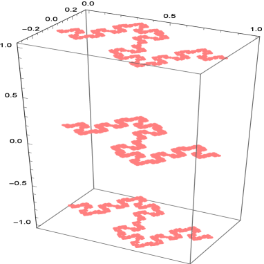
Figure 11: The graph of the first eigenfunction

Figure 12: The graph of the second eigenfunction

Figure 13: The graph of the third eigenfunction

Figure 14: The graph of the fourth eigenfunction

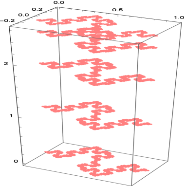
Figure 15: The graph of the fifth eigenfunction

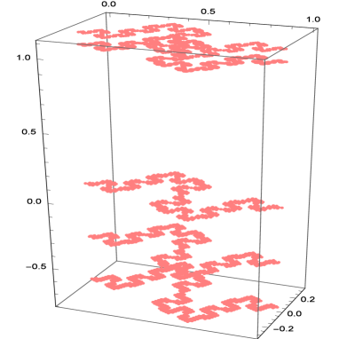
Figure 16: The graph of the sixth eigenfunction

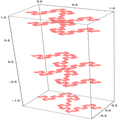
Figure 17: The graph of the seventh eigenfunction

7 Metric - Towards spectral asymptotics

Definition 7.1.

Effective resistance metric, on ${\mathfrak{MC}}$
Given two points $(X,Y)$ of ${\mathfrak{MC}}^{2}$, let us introduce the effective resistance metric between $X$ and $Y$:

$$R_{\mathfrak{MC}}(X,Y)=\left\{\min_{\left\{u\,|\,u(X)=0,u(Y)=1\right\}}\,{\cal E}(u)\right\}^{-1}$$

In an equivalent way, $R_{\mathfrak{MC}}(X,Y)$ can be defined as the minimum value of the real numbers $R$ such that, for any function $u$ of $\text{dom}\,\Delta$:

$$\left|u(X)-u(Y)\right|^{2}\leqslant R\,{\cal E}(u)$$

Definition 7.2.

Metric, on the Minkowski Curve ${\mathfrak{MC}}$
Let us define, on the Minkowski Curve ${\mathfrak{MC}}$, the distance $d_{\mathfrak{MC}}$ such that, for any pair of points $(X,Y)$ of ${\mathfrak{MC}}^{2}$:

$$d_{{\mathfrak{MC}}}(X,Y)=\left\{\min_{\left\{u\,|\,u(X)=0,u(Y)=1\right\}}\,{\cal E}(u,u)\right\}^{-1}$$

Remark 7.1.

One may note that the minimum

$$\min_{\left\{u\,|\,u(X)=0,u(Y)=1\right\}}\,{\cal E}(u)$$

is reached for $u$ being harmonic on the complement set, on $\mathfrak{MC}$, of the set

$$\left\{X\right\}\cup\left\{Y\right\}$$

(One might bear in mind that, due to its definition, a harmonic function $u$ on $\mathfrak{MC}$ minimizes the sequence of energies $\left({\cal E}_{{\mathfrak{MC}}_{m}}(u,u)\right)_{m\in{\mathbb{N}}}$.

Definition 7.3.

Dimension of the Minkowski Curve ${\mathfrak{MC}}$, in the resistance metrics

The dimension of the Minkowski Curve ${\mathfrak{MC}}$, in the resistance metrics, is the strictly positive number $d_{\mathfrak{MC}}$ such that, given a strictly positive real number $r$, and a point $X\,\in\,{\mathfrak{MC}}$, for the $X-$centered ball of radius $r$, denoted by ${\cal B}_{r}(X)$:

$$\mu\left({\cal B}_{r}(X)\right)=r^{d_{\mathfrak{MC}}}$$

Property 7.1.

Given a natural integer $m$, and two points $(X,Y)$ of ${\mathfrak{MC}}^{2}$ such that $X\underset{m}{\sim}Y$:

$$\min_{\left\{u\,|\,u(X)=0,u(Y)=1\right\}}\,{\cal E}(u)\lesssim r^{m}\,4^{-2\,m\,\delta}=\displaystyle\frac{1}{8^{m}}$$

Let us denote by $\mu$ the standard measure on $\mathfrak{MC}$ which assigns measure $\displaystyle\frac{1}{4^{2m}}$ to each quadrilateral $m-$ cell. Let us now look for a real number $d_{\mathfrak{MC}}$ such that:

$$\left(\displaystyle\frac{1}{8}\right)^{m\,d_{\mathfrak{MC}}}=\displaystyle\frac{1}{4^{2m}}$$

One obtains:

$$d_{\mathfrak{MC}}=\displaystyle\frac{2}{3}$$

Given a strictly positive real number $r$, and a point $X\,\in\,{\mathfrak{MC}}$, one has then the following estimate, for the $X-$centered ball of radius $r$, denoted by ${\cal B}_{r}(X)$:

$$\mu\left({\cal B}_{r}(X)\right)=r^{d_{\mathfrak{MC}}}$$

Definition 7.4.

Eigenvalue counting function

We introduce the eigenvalue counting function ${\cal N}^{\mathfrak{MC}}$ such that, for any real number $x$:

$${\cal N}^{\mathfrak{MC}}(x)=\#\,\left\{\lambda\,\text{eigenvalue of $-\Delta$}\,:\quad\lambda\leqslant x\right\}$$

Property 7.2.

According to J. Kigami [Kig98], one has the modified Weyl formula:

$${\cal N}^{\mathfrak{MI}}(x)=\left(G\left(\frac{\ln x}{2}\right)+o(1)\right){x^{D_{S}\left(\mathfrak{MI}\right)}}$$

8 From the Minkowski Curve, to the Minskowski Island

By connecting four Minkowski Curves, as it can be seen on the following figure:

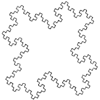
Figure 18: The Minskowski Island.

one obtains what is called "the Minskowski Island".

We expose, in the sequel, our results (we refer to Zhou [Zho07] for further details).
In the case of the Minkowski Curve, one may check that:

$$\#(F_{i}(V_{0})\cap V_{0})\leqslant 1\quad\forall\ i\in\{1,2,3,4,5,6,7,8\}$$

$$D=\left(\begin{array}[]{cccc}-2&1&0&1\\ 1&-2&1&0\\ 0&1&-2&1\\ 1&0&1&-2\\ \end{array}\right)\quad,\quad T=\left(\begin{array}[]{cccc}-2&0&0&0\\ 0&-2&0&0\\ 0&0&-2&0\\ 0&0&0&-2\\ \end{array}\right)$$

Let us set:

$$B=\left(\begin{array}[]{ccccccc}-2&1&0&0&0&0&0\\ 1&-2&1&0&0&0&0\\ 0&1&-2&1&0&0&0\\ 0&0&1&-2&1&0&0\\ 0&0&0&1&-2&1&0\\ 0&0&0&0&1&-2&1\\ 0&0&0&0&0&1&-2\\ \end{array}\right)$$

and:

$$C=\left(\begin{array}[]{ccccccc}2&0&0&0&0&0&0\\ 0&2&0&0&0&0&0\\ 0&0&2&0&0&0&0\\ 0&0&0&2&0&0&0\\ 0&0&0&0&2&0&0\\ 0&0&0&0&0&2&0\\ 0&0&0&0&0&0&2\\ \end{array}\right)$$

Then:

$$X=\left(\begin{array}[]{cccc}B&0&0&0\\ 0&B&0&0\\ 0&0&B&0\\ 0&0&0&B\\ \end{array}\right)$$

and:

$$M=\left(\begin{array}[]{cccc}C&0&0&0\\ 0&C&0&0\\ 0&0&C&0\\ 0&0&0&C\\ \end{array}\right)\quad,\quad J=\left(\begin{array}[]{cccc}1&0&0&0\\ 0&0&0&0\\ 0&0&0&0\\ 0&0&0&0\\ 0&0&0&0\\ 0&0&0&0\\ 0&1&0&0\\ 0&1&0&0\\ 0&0&0&0\\ 0&0&0&0\\ 0&0&0&0\\ 0&0&0&0\\ 0&0&0&0\\ 0&0&1&0\\ 0&0&1&0\\ 0&0&0&0\\ 0&0&0&0\\ 0&0&0&0\\ 0&0&0&0\\ 0&0&0&0\\ 0&0&0&1\\ 0&0&0&1\\ 0&0&0&0\\ 0&0&0&0\\ 0&0&0&0\\ 0&0&0&0\\ 0&0&0&0\\ 1&0&0&0\\ \end{array}\right)$$

One may check that the Minkowsky Island has a strong harmonic structure, and that:

$$T+J^{T}\,(X+\lambda M)^{-1}J=-\frac{1}{8(\lambda-1)\,(2\,(\lambda-2)\,\lambda+1)\left(8\,(\lambda-2)\lambda\,(\lambda-1)^{2}+1\right)}\,D+\frac{\lambda\,(4\,\lambda(\lambda(2\lambda-7)+7)-7)}{8\,(\lambda-2)\lambda\,(\lambda-1)^{2}+1}\,T$$

We obtain, as previously:

$$\frac{1}{K_{D}(0)}=8$$

The spectral decimation function is given, for any real number $\lambda$, by:

$$R(\lambda)=-(\lambda-4)(\lambda-2)^{2}\lambda((\lambda-4)\lambda+2)^{2}$$

which leads to the same spectrum as the one of the Curve.

References

- [BD85] A. Beurling and J. Deny. Espaces de Dirichlet. i. le cas élémentaire. Annales scientifiques de l’É.N.S. 4 e série, 99(1):203–224, 1985.
- [Cap02] R. Capitanelli. Nonlinear energy forms on certain fractal curves. J. Nonlinear Convex Anal., 3(1):67–80, 2002.
- [FL04] U. R. Freiberg and M. R. Lancia. Energy form on a closed fractal curve. Journal for Analysis and its Applications, 23(1):115–137, 2004.
- [FS92] M. Fukushima and T. Shima. On a spectral analysis for the Sierpiński gasket. Potential Anal, 1:1–3, 1992.
- [FT13] U. R. Freiberg and C. Thäle. Exact Computation and Approximation of Stochastic and Analytic Parameters of Generalized Sierpinski Gaskets. C. Methodol. Comput. Appl. Probab., 15(3):485–509, 2013.
- [Har93] J. Harrison. Stokes theorem for nonsmooth chains. Bull. of AMS, 29(2):235–242, 1993.
- [HN91] J. Harrison and A. Norton. Geometric integration on fractal curves in the plane. Bull. of AMS, 402:567–594, 1991.
- [HN92] J. Harrison and A. Norton. The Gauss-Green theorem for fractal boundaries. Duke Math. J., 673:575–586, 1992.
- [Hut81] J. E. Hutchinson. Fractals and self similarity. Indiana University Mathematics Journal, 30:713–747, 1981.
- [Kig89] J. Kigami. A harmonic calculus on the Sierpiński spaces. Japan J. Appl. Math., 8:259–290, 1989.
- [Kig93] J. Kigami. Harmonic calculus on p.c.f. self-similar sets. Trans. Amer. Math. Soc., 335:721–755, 1993.
- [Kig98] J. Kigami. Distributions of localized eigenvalues of laplacians on post critically finite self-similar sets. Journal of Functional Analysis, 156(1):170–198, 1998.
- [Kig03] J. Kigami. Harmonic analysis for resistance forms. Journal of Functional Analysis, 204:399–444, 2003.
- [KS83] J. G. Kemeny and J. Laurie Snell. Finite Markov chains. Springer, 3rd printing 1983 edition, 1983.
- [Man77] B. B. Mandelbrot. Fractals: form, chance, and dimension. San Francisco: Freeman, 1977.
- [Mos02] Umberto Mosco. Energy functionals on certain fractal structures. Journal of Convex Analysis, 9(2):581–600, 2002.
- [Sab97] C. Sabot. Existence and uniqueness of diffusions on finitely ramified self-similar fractals. Annales scientifiques de l’É.N.S. 4 e série, 30(4):605–673, 1997.
- [Str99] R. S. Strichartz. Analysis on fractals. Notices of the AMS, 46(8):1199–1208, 1999.
- [Str06] R. S. Strichartz. Differential Equations on Fractals, A tutorial. Princeton University Press, 2006.
- [UD14] R. Uthayakumar and A. N. Nalayini Devi. Some properties on Koch curve. In C. Bandt, M. Barnsley, R. Devaney, K. Falconer, V. Kannan, P. B. Kumar (eds), Fractals, Wavelets, and their Applications. Springer Proceedings in Mathematics & Statistics, 2014.
- [Zho07] Denglin Zhou. Spectral Analysis of Laplacians on Certain Fractals. PhD thesis, University of Waterloo, 2007.