Large magnetic field variations towards the Galactic Centre magnetar, PSR J1745$-$2900

Abstract

Polarised radio emission from PSR J1745$-$2900 has already been used to investigate the strength of the magnetic field in the Galactic Centre, close to Sagittarius A*. Here we report how persistent radio emission from this magnetar, for over four years since its discovery, has revealed large changes in the observed Faraday rotation measure, by up to 3500 rad m^-2 (a five per cent fractional change). From simultaneous analysis of the dispersion measure, we determine that these fluctuations are dominated by variations in the projected magnetic field, rather than the integrated free electron density, along the changing line of sight to the rapidly moving magnetar. From a structure function analysis of rotation measure variations, and a recent epoch of rapid change of rotation measure, we determine a minimum scale of magnetic fluctuations of size $\sim 2$ au at the Galactic Centre distance, inferring PSR J1745$-$2900 is just $\sim 0.1$ pc behind an additional scattering screen.

1 Introduction

Measurements of Faraday Rotation in the polarised emission of radio sources can be used to examine the strength and structure of the magnetic field in the interstellar medium (Beck & Wielebinski, 2013). A recent notable example is the radio-loud magnetar, PSR J1745$-$2900, which displays a high rotation measure (RM) of $-66960\pm 50$ rad m^-2, second only in the Galaxy to the $\text{RM}=(-4.3\pm 0.1)\times 10^{5}$ rad m^-2 of the supermassive black hole candidate, Sagittarius A^∗ (Sgr A^∗), caused predominantly by the accretion flow on scales smaller than the Bondi-Hoyle radius (Bower et al., 2003). This magnetar therefore allowed first-order estimates of the strength of the magnetic field at the beginnings of the Bondi-Hoyle accretion radius of Sgr A^∗; $\sim 8$ mG at scales of $\sim 0.1$ pc (Eatough et al., 2013). The magnitude and spatial or time variability of the magnetic field also allows models of the accretion flow to be investigated (Pang et al., 2011).

PSR J1745$-$2900 has also been used to examine the scattering of radio waves towards the Galactic Centre (GC) by measurements of both the temporal pulse broadening (Spitler et al., 2014) and the angular image broadening (Bower et al., 2014). Combination of the two measurements indicates the principal scattering screen toward the GC is $5.8\pm 0.3\,\text{kpc}$ in front of the magnetar (Bower et al., 2014).

Atypically for magnetars, PSR J1745$-$2900 has remained active in the radio band for over four years since its discovery at X-ray wavelengths in 2013 (Kennea et al., 2013; Mori et al., 2013). This has allowed repeated measurements of the RM and dispersion measure (DM). Because the magnetar has a total proper motion of $6.37\pm 0.16$ mas yr^-1 (Bower et al., 2015), the time-variations in the measurements of DM and RM presented here occur along different sightlines. The physical scales probed in the GC are therefore directly related to the observing cadence, and the transverse velocity of the magnetar.

In this paper, long term polarimetric observations of PSR J1745$-$2900 with the Effelsberg and Nançay radio telescopes are presented. Section 2 gives a description of the observational campaign and data analysis techniques used. In Section 3 the results of the analysis are presented, and in Section 4 we turn to physical interpretations of the results.

2 Observations

Following the discovery of radio pulsations from PSR J1745$-$2900 in April 2013, this source has been monitored with three European radio telescopes operating at complementary observing frequencies. These are the Effelsberg radio telescope, the Nançay Radio Telescope (NRT) and the Jodrell Bank, Lovell radio telescope. In this work we only refer to measurements from the Effelsberg telescope and the NRT because observations with the Lovell telescope, at a lower frequency of 1.4 GHz, suffer from instrumental depolarisation due to the large RM.

2.1 Effelsberg

PSR J1745$-$2900 is observed with the Effelsberg telescope typically on a monthly basis, and fortnightly since January 2017. One-hour observations at central frequencies of 8.35 GHz and 4.85 GHz are recorded with the PSRIX backend (Lazarus et al., 2016).

The 500 MHz bandwidth provided by the PSRIX backend is first digitised and split into 512 or 1024 channels when observing at 8.35 GHz and 4.85 GHz, respectively. The channelised data are then dedispersed at a DM of 1778 pc cm^-3, the initial value DM measured by Eatough et al. (2013) and finally folded at the period of the magnetar to create ‘single pulse profiles’.

Since March 2017 the new ‘C+’ broadband receiver is available for pulsar observations. Two 2 GHz bands (covering 4 to 8 GHz) are fed into the new PSRIX2 backend, consisting of two CASPER ROACH2 boards. Each board digitises the signal and acts as a full-Stokes spectrometer, creating 2048 frequency channels every 8 $\mu$s. The data are later dedispersed and folded to create single pulses profiles. During the commissioning phase of PSRIX2, the C+ observations replace the 8.35 GHz observations.

2.2 Nançay

Observations with the NRT were carried out with the NUPPI instrumentation on average every 4 days between May 2013 and August 2014, before resuming at a monthly cadence between January and July 2017. The setup of the observations was already presented in Eatough et al. (2013); Spitler et al. (2014); Torne et al. (2015). We briefly summarize it here. A bandwidth of 512 MHz centred at 2.5 GHz is split into 1024 channels and coherently dedispersed using an initial DM value of 1840 pc cm^-3 (the best DM value derived from timing of the scattered pulse profiles) then folded at the period of the magnetar and written to disk every 30 s.

2.3 Post-processing and calibration

All the data presented here are corrected for the gain and phase difference between the feeds of the various receivers used. This is achieved by standard pulsar calibration techniques that use observations of a polarised pulsed noise diode. Large $|$RM$|$s, in combination with wide frequency channels, lead to instrumental depolarization. Following the analysis presented in Schnitzeler & Lee (2015), we calculate that an $|$RM$|$ of $7\times 10^{4}$ rad m^-2 depolarizes the signal by only 4 per cent in the 2.5 GHz band; at the higher observing frequencies, this effect is negligible. The data reduction is achieved with the standard PSRCHIVE package (Hotan et al., 2004).

3 Results

Monitoring of the dispersive and polarisation properties of PSR J1745$-$2900 over a period of $\sim 54$ months has revealed a rather constant DM of $1762\pm 11$ cm pc^-3, while variations in RM $>3500$ rad m^-2 are observed. Because RM is proportional to both projected magnetic field strength $B_{\mathbin{\!/\mkern-5.0mu/\!}}$, and the free electron density $n_{\textrm{e}}$, along the line-of-sight $s$, ${\rm RM}\propto\int B_{\mathbin{\!/\mkern-5.0mu/\!}}(s)n_{\textrm{e}}(s)\text{d}s$, it is important to disentangle these quantities to understand the physical mechanisms causing the variations in RM. For PSR J1745$-$2900, which has the highest DM amongst all the known pulsars, measurement of the DM is influenced by pulse scattering. In this section the methods used to measure both the DM and RM are described, as well as the results of our monitoring campaign.

3.1 Dispersion Measure variations

To accurately measure the DM and remove the bias caused by the scattering of the pulse profile (and possibly the variations of it), we modelled both scattering and DM simultaneously over a range of frequency subbands for each NUPPI, PSRIX and PSRIX2 observations. Given the low amount of dispersion across the band of the PSRIX data at 8.35 GHz ($\sim 12$ ms), we did not apply this technique to these data.

Following Spitler et al. (2014), we use scattered Gaussian pulse function to model the single pulses observed between 4 and 8 GHz and the averaged pulse profile at 2.5 GHz. However, in contrast to Spitler et al. (2014), we did not correct for the jittering of the single pulses to create an average ‘de-jittered’ profile. Instead, we model simultaneously some of the brightest single pulses in each observation with different Gaussian widths $\sigma$ to increase the significance of our results.

The scattered Gaussian pulse profile function for a single channel is given by Equation 3 of Spitler et al. (2014). We extend it here for multiple channels to include the DM as a parameter. We can therefore write the likelihood $\Lambda$ as

$$\log\Lambda=\frac{1}{2}\sum_{i}^{N_{\text{p}}}\sum_{j}^{N_{\text{c}}}\sum_{k}^{N_{\text{b}}}\left\{P_{ijk}-T_{ijk}\right\}+\text{const},$$ (1)

where $P_{ijk}$ is the observed single pulse profile $i$ with frequency channel $j$ and profile bin $k$ over $N_{\text{p}}$ profiles included in the modelling with $N_{\text{c}}$ frequency channels and $N_{\text{b}}$ phase bins. $T_{ijk}$ is the modelled scattered profile,

$$T_{ijk}=\frac{A_{ij}\sqrt{\pi}}{2}\sigma_{i}e^{\frac{\sigma_{i}^{2}-4\phi_{ijk}\tau}{4\tau^{2}}}\\ \times\left\{1+\text{erf}\left(\frac{2\tau(\phi_{ijk}-\phi_{0,ij})-\sigma_{i}^{2}}{2\tau\sigma_{i}}\right)\right\}+b_{ij}.$$ (2)

$A_{ij}$ and $b_{ij}$ are, respectively, the amplitude and the baseline offset of channel $j$ from profile $i$. $\phi_{0,ij}$ is the phase centre of the Gaussian of width $\sigma_{i}$, but delayed in each channel because of dispersion. $\phi_{0,ij}$ is given by $\phi_{0,ij}=\phi_{0,i}+k\text{DM}\times(1/f_{i}^{2}-1/f_{0}^{2})$, where the dispersion constant $k=4.15\times 10^{3}$ MHz² cm³ pc^-1 s. Finally, $\tau$ is the scattering time at a reference frequency $f_{0}$. The dimensionality of the model is therefore $2+N_{\text{p}}\times(2+2\times N_{\text{c}})$, where $N_{\text{p}}$ is 1 for the NRT averaged profile, typically 2 to 4 for the Effelsberg single pulse observations and $N_{\text{c}}$ range from 8 to 16.

Given the large dimensionality of the model, we implemented the nested sampling tool POLYCHORD (Handley et al., 2015) to efficiently sample the parameter space instead of using traditional $\chi^{2}$-fitting techniques. The priors on all parameters are set to be uniform, except for $A_{ij}$ where we use log-uniform priors. We refer to one-sigma error bars as the 68.3 per cent contours of the one-dimensional marginalized posterior distribution of each parameter. The resulting code can be found online. An example of our modelling results can be seen in Figure 1.

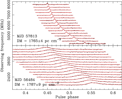
Figure 1: Scattered and dispersed observed pulse profiles of PSR J1745$-$2900 (over a selected phase window) are shown in black color for a set of 16 subbands from a C+ single pulse profile (top panel) and a 2.5 GHz daily averaged profile (bottom panel). The red curves show our model of scattered and dispersed Gaussian profiles taken from the maximum likelihood solution. The MJD of the observation and the estimated DM are indicated at the bottom-left part of each panel.

The DM results of the modelling of the Effelsberg and NRT data are shown in Figure 2. A linear least-squares fit to the DM values shows a marginal decrease of approximately 0.6 per cent over four years (two-sigma consistent with no DM change) with DM=$1762\pm 11$ cm pc^-3 as measured in October 2017. Results from the scattering measurements that come out of this joint analysis will be published elsewhere.

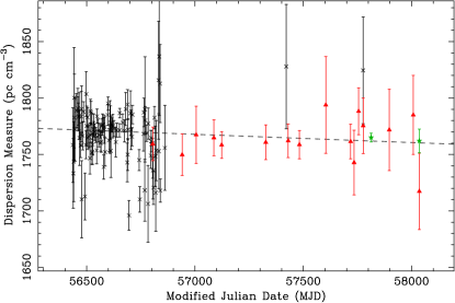
Figure 2: DM variations of the GC magnetar. The black crosses, red triangles and green stars show the DM values (with one-sigma error bars) from the modelling of the scattered profiles from the 2.5 GHz, 4.85 GHz and C+ data, respectively. The dashed line represents the linear least-squares fit to the data. The MJD and modelled DM are reported in the bottom-left part of each panel.

3.2 Rotation Measure variations

To determine the Faraday rotation of the linearly polarised emission of the magnetar, we used the RM synthesis method (Brentjens & de Bruyn, 2005) and fitted the wrapping of the Stokes vector Q and U under the pulse window as previously done in Eatough et al. (2013). We employed this technique to extract the RM for all our data. In contrast to our DM results, Figure 3 shows the rapid and non-monotonic evolution of the RM during our 4 years of observations. Since the initial $\text{RM}=-66960\pm 50$ rad m^-2 reported in Eatough et al. (2013), the RM changed by over 3500 units to $\text{RM}=-63402\pm 232$ rad m^-2 in October 2017 (a relative change of 5.3 per cent). Our measurements are also consistent with the $\text{RM}=-66080\pm 24$ rad m^-2 reported by Schnitzeler et al. (2016) using Australian Telescope Compact Array (ATCA) observations at 5.4 GHz. After a steady increase in the first few months, the RM increased abruptly around MJD 56566 followed by another steady increase until MJD 57450. Then the RM diminished up to MJD 57600 before increasing over the last year of observations. A least-squares fit to the data collected over the last year shows that RM changed by about $7.4$ rad m^-2 per day. It is worth noting that two-weeks of follow-up observations of the magnetar SGR 1806$-$20 after an outburst phase did not show evidence for RM variations (Gaensler et al., 2005).

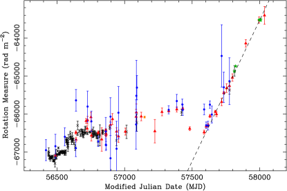
Figure 3: Variation of RM as a function of MJD. The black crosses, red triangles, blue points and green stars show the RM values estimated from the 2.5 GHz, 4.85 GHz, 8.35 GHz and C+ data, respectively. The orange rectangle shows the value from the ATCA data recorded at 5.4 GHz (Schnitzeler et al., 2016). The black dashed line shows the fitted slope of the recent epoch of large gradient in RM variation.

3.3 Polarisation fraction

Figure 4 shows the evolution of the linear polarisation fraction $L_{\text{f}}$ as a function of time for all our data. These results show large variations in $L_{\text{f}}$ at all frequencies, with $L_{\text{f}}$ at 2.5 GHz consistently lower than at higher frequencies, by a factor of between 2 and 10.

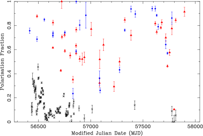
Figure 4: Polarisation fraction as a function of time. The black crosses, red triangles and blue points show the values from the 2.5 GHz, 4.85 GHz and 8.35 GHz data, respectively. The polarisation fraction at 2.5 GHz is consistently lower than at the higher frequencies.

4 Discussion

The observations presented here show a clear dichotomy between the properties of the DM and RM variations toward PSR J1745$-$2900; the DM varies marginally while the RM shows very large variations. This is not entirely unexpected since it has been suggested that the RM is likely caused by local magnetic phenomena, somewhere in the last few parsecs toward the GC, whereas most of the DM is accumulated along the entire line of sight to the magnetar (Eatough et al., 2013). We note the RM variations observed are three orders of magnitude above what might be expected from ionospheric contributions (Yan et al., 2011).

4.1 Structure function analysis

As already mentioned, PSR J1745$-$2900 has a proper motion (Bower et al., 2015), so our measurements of DM and RM can be used to probe the angular and physical scales on which these fluctuations occur. For sparsely and irregularly sampled data, like these, power spectrum analyses are unsuitable. A frequently used alternative is the structure function of variations, see e.g. Minter & Spangler (1996). Following their notation, the ensemble average second order structure function in DM and RM can be written ${\rm SF}_{\rm DM}=\langle[{\rm DM}(\theta)-{\rm DM}({\theta}+\delta{\theta})]^{2}\rangle$ and ${\rm SF}_{\rm RM}=\langle[{\rm RM}(\theta)-{\rm RM}({\theta}+\delta{\theta})]^{2}\rangle$, respectively, where ${\theta}$ is any given line of sight and $\delta\theta$ is the angular separation or ‘lag’ of two measurements. In this work the lag is given by the total magnitude of the proper motion (6.37 mas yr^-1) multiplied by the separation in time of two DM or RM measurements. In addition, we corrected each pair of DM and RM used in the structure function for noise bias, by subtracting ($\delta\textrm{DM}(\theta)^{2}+\delta\textrm{DM}({\theta}+\delta{\theta})^{2}$) and ($\delta\textrm{RM}(\theta)^{2}+\delta\textrm{RM}({\theta}+\delta{\theta})^{2}$), respectively. In Figure 5 we present the results from the structure function analysis. In the top panel, averaged values of ${\rm SF}_{\rm DM}$ are unchanging across all angular scales from ${10^{-10}}$ deg to ${10^{-5}}$ deg. This is representative of the flat fit of the DM time series in Section 3.1. The bottom panel of Figure 5 shows ${\rm SF}_{\rm RM}$ over the same interval in angular scale. Unlike ${\rm SF}_{\rm DM}$, ${\rm SF}_{\rm RM}$ begins rising at angular scales over ${10^{-8}}$ deg, equivalent to a physical size of a few au at a GC distance of $8.3$ kpc (Gillessen et al., 2009). We define this size as the approximate smallest-scale at which magnetic structure in the GC is observed in our data.

The fitted slope of ${\rm SF}_{\rm RM}$ (black dashed line), $l=1.23\pm 0.13$, is potentially indicative of Kolmogorov turbulence (where $l=5/3$) assuming isotropic and stationary fluctuations in RM (Simonetti et al., 1984; Lazio et al., 1990; Haverkorn et al., 2004).

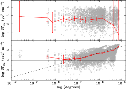
Figure 5: Structure functions, corrected for measurement errors, for the DM (top panel) and RM (bottom panel). For clarity, the error bars for each lag (grey crosses) are not shown. The red points represent the averaged values over intervals of 0.25 in log scale. The horizontal black line delimits RM variations of 100 rad m^-2. The black dashed line shows the linear fit to the average values of ${\rm SF}_{\rm RM}$ allowing to give an estimate on the angular scale at which the RM variations occur.

4.2 A physical model based on the depolarisation

Figure 4 shows that PSR J1745$-$2900 depolarises rapidly with decreasing frequency. This could be intrinsic to the magnetar, or caused by a propagation effect. Because the former has not been observed in magnetars (e.g. Kramer et al., 2007), in this section we model depolarisation due to propagation through the interstellar medium.

For this purpose we invoke a secondary scattering screen, close to the magnetar in the GC, in addition to the distant screen ($\sim 6$ kpc from the GC) responsible for the temporal scatter broadening (Bower et al., 2014; Wucknitz, 2014). The distant screen cannot produce the rapid RM variations we observe due to its large size (160 mas at 2.5 GHz) because spiral arms do not host strong magnetic fields (Haverkorn, 2015). Scattering screens located close to the GC (<700 pc) have been previously indicated for other GC pulsars (Dexter et al., 2017). As the magnetar moves behind or through a magnetized, ionized gas, the variation in RM that we observe over time also imprints itself as a gradient in RM across this secondary scattering disk. Following Schnitzeler et al. (2015), we can show that RM variations of order 100 rad m^-2 within a scattering disk (Gaussian disk with a FWHM of 0.2-0.5 mas or a uniformly lit circular disk with diameter $<$ 1 mas at 2.5 GHz) is enough to explain little or no depolarization at the highest observing frequencies, and the strong or even complete depolarization at 2.5 GHz. At this frequency an RM gradient of $100$ rad m^-2 across the scattering disk would lead to PA differences up to $\sim 80$ deg, leading to strong depolarisation.

By considering both measurements from the RM structure function analysis outlined in Section 4.1, and the recently measured large gradient in RM (the fitted slope described in Section 3.2), fluctuations of order $100$ rad m^-2 are readily observable in our data set and occur at angular-scales, or time-scales, of the order tenths of milliarcseconds and weeks respectively.

The solid horizontal black line at ${\rm SF}_{\rm RM}=10000\,{\rm rad^{2}\,m^{-4}}$ in Figure 5 defines the limit where changes in RM of 100 rad m^-2 occur. The intercept of this line with the fitted averages of ${\rm SF}_{\rm RM}$ gives the approximate angular scale at which these fluctuations begin to occur; which is around $6\times 10^{-8}$ deg ($\sim 0.22$ mas or a physical scale of $\sim 1.8$ au at a GC distance of 8.3 kpc). The fitted slope in RM in Figure 3 indicates a change in RM of 100 rad m^-2 occurs on time-scales of just two weeks (angular displacement of $\sim 0.24$ mas, physical scale of $\sim 2.0$ au at distance of 8.3 kpc). Much shorter term variations ($<1$ hr) have been ruled out. The average value of these two measured physical scales maps to an upper bound on the scattering disk size $b$ of $\sim 1.9$ au.

The geometric scattering time delay, $\tau$, depends upon both the magnetar’s distance to the screen, $z$, and its size, $b$, through $\tau=b^{2}/2cz$. $\tau$ is bounded by the observed scattering time at 2.5 GHz, and is likely substantially shorter since most of the scattering delay occurs at the midway screen (Wucknitz, 2014). Following Spitler et al. (2014) we use $\tau<0.04$ s giving $z\gtrsim 0.1$ pc. Remarkably, this places the secondary scattering screen at least 0.1 pc in front of PSR J1745$-$2900, the same distance as the projected offset from Sgr A^∗; therefore placing the screen close to the Bondi-Hoyle accretion radius. The observed fluctuations in magnetic field are thus potentially occurring within the black hole reservoir. The two main assumptions in this model are the isotropy of the RM variations, and the attribution of depolarisation to propagation effects.

The constancy in electron density toward PSR J1745$-$2900, indicated by our DM measurements, therefore suggests an additional scattering screen local to the GC and embedded in a strong ambient magnetic field ($\sim 8$ mG; Eatough et al., 2013). Fluctuations in this field, of $\sim 12\,\mu$G starting at sizes of $\sim 2$ au and going up to $\sim 400\,\mu$G on the largest measured scales of $\sim 300$ au occur either due to changes in its strength or orientation. Our data also suggest the RM fluctuations are potentially Kolmogorov in nature.

Future observations of PSR J1745$-$2900 will better constrain the magnetic field structure around Sgr A^∗ and can potentially be used to test if the accretion flow becomes magnetically dominated (Pen et al., 2003).

References

- Beck & Wielebinski (2013) Beck R., Wielebinski R., 2013, Magnetic Fields in Galaxies. p. 641
- Bower et al. (2003) Bower G. C., Wright M. C. H., Falcke H., Backer D. C., 2003, ApJ, 588, 331
- Bower et al. (2014) Bower G. C., et al., 2014, ApJ, 780, L2
- Bower et al. (2015) Bower G. C., et al., 2015, ApJ, 798, 120
- Brentjens & de Bruyn (2005) Brentjens M. A., de Bruyn A. G., 2005, A&A, 441, 1217
- Dexter et al. (2017) Dexter J., et al., 2017, MNRAS, 471, 3563
- Eatough et al. (2013) Eatough R. P., et al., 2013, Nature, 501, 391
- Gaensler et al. (2005) Gaensler B. M., et al., 2005, Nature, 434, 1104
- Gillessen et al. (2009) Gillessen S., Eisenhauer F., Fritz T. K., Bartko H., Dodds-Eden K., Pfuhl O., Ott T., Genzel R., 2009, ApJ, 707, L114
- Handley et al. (2015) Handley W. J., Hobson M. P., Lasenby A. N., 2015, MNRAS, 453, 4384
- Haverkorn (2015) Haverkorn M., 2015, in Lazarian A., de Gouveia Dal Pino E. M., Melioli C., eds, Astrophysics and Space Science Library Vol. 407, Magnetic Fields in Diffuse Media. p. 483 (arXiv:1406.0283)
- Haverkorn et al. (2004) Haverkorn M., Gaensler B. M., McClure-Griffiths N. M., Dickey J. M., Green A. J., 2004, ApJ, 609, 776
- Hotan et al. (2004) Hotan A. W., van Straten W., Manchester R. N., 2004, PASA, 21, 302
- Kennea et al. (2013) Kennea J. A., et al., 2013, ApJ, 770, L24
- Kramer et al. (2007) Kramer M., Stappers B. W., Jessner A., Lyne A. G., Jordan C. A., 2007, MNRAS, 377, 107
- Lazarus et al. (2016) Lazarus P., Karuppusamy R., Graikou E., Caballero R. N., Champion D. J., Lee K. J., Verbiest J. P. W., Kramer M., 2016, MNRAS, 458, 868
- Lazio et al. (1990) Lazio T. J., Spangler S. R., Cordes J. M., 1990, ApJ, 363, 515
- Minter & Spangler (1996) Minter A. H., Spangler S. R., 1996, ApJ, 458, 194
- Mori et al. (2013) Mori K., et al., 2013, ApJ, 770, L23
- Pang et al. (2011) Pang B., Pen U.-L., Matzner C. D., Green S. R., Liebendörfer M., 2011, MNRAS, 415, 1228
- Pen et al. (2003) Pen U.-L., Matzner C. D., Wong S., 2003, ApJ, 596, L207
- Schnitzeler & Lee (2015) Schnitzeler D. H. F. M., Lee K. J., 2015, MNRAS, 447, L26
- Schnitzeler et al. (2015) Schnitzeler D. H. F. M., Banfield J. K., Lee K. J., 2015, MNRAS, 450, 3579
- Schnitzeler et al. (2016) Schnitzeler D. H. F. M., Eatough R. P., Ferrière K., Kramer M., Lee K. J., Noutsos A., Shannon R. M., 2016, MNRAS, 459, 3005
- Simonetti et al. (1984) Simonetti J. H., Cordes J. M., Spangler S. R., 1984, ApJ, 284, 126
- Spitler et al. (2014) Spitler L. G., et al., 2014, ApJ, 780, L3
- Torne et al. (2015) Torne P., et al., 2015, MNRAS, 451, L50
- Wucknitz (2014) Wucknitz O., 2014, in Proceedings of the 12th European VLBI Network Symposium and Users Meeting (EVN 2014), Cagliari, Italy.. p. 66
- Yan et al. (2011) Yan W. M., et al., 2011, Ap&SS, 335, 485