Hyperasymptotics and quark-hadron duality violations in QCD

Diogo Boito,^a Irinel Caprini,^b Maarten Golterman,^c,d Kim Maltman,^e,f Santiago Peris^c

^aInstituto de Física de São Carlos, Universidade de São Paulo, CP 369
13570-970, São Carlos, SP, Brazil
^bHoria Hulubei National Institute for Physics and Nuclear Engineering, POB MG-6
077125 Bucharest-Magurele, Romania
^cDepartment of Physics and IFAE-BIST, Universitat Autònoma de Barcelona
E-08193 Bellaterra, Barcelona, Spain
^dDepartment of Physics and Astronomy, San Francisco State University
San Francisco, CA 94132, USA
^eDepartment of Mathematics and Statistics, York University
Toronto, ON Canada M3J 1P3
^fCSSM, University of Adelaide, Adelaide, SA 5005 Australia

We investigate the origin of the quark-hadron duality-violating terms in the expansion of the QCD two-point vector correlation function at large energies in the complex $q^{2}$ plane. Starting from the dispersive representation for the associated polarization, the analytic continuation of the operator product expansion from the Euclidean to the Minkowski region is performed by means of a generalized Borel-Laplace transform, borrowing techniques from hyperasymptotics. We establish a connection between singularities in the Borel plane and quark-hadron duality violating contributions. Starting with the assumption that for QCD at $N_{c}=\infty$ the spectrum approaches a Regge trajectory at large energy, we obtain an expression for quark-hadron duality violations at large, but finite $N_{c}$.

1 Introduction

Correlation functions in QCD, at sufficiently large energy, can be calculated starting from the gluon and quark degrees of freedom, using perturbation theory, augmented by the operator product expansion (OPE). Many of these correlators, such as the Adler function of the vector current two-point function, can also be expressed, through dispersion relations, in terms of experimentally accessible spectral functions. These spectral functions reveal the presence of multiple hadronic resonances, whose spectral contributions are not reproduced when perturbative and higher-dimension OPE contributions are evaluated on the Minkowski axis.

In spite of this difference, a complete description in terms of Lagrangian or physical degrees of freedom should be equivalent, a notion which is referred to as quark-hadron duality. It is, however, generally accepted that even at large energies, resonance effects, and hence contributions beyond the OPE, are present in QCD correlators in the Minkowski region. These additional contributions, which by definition violate quark-hadron duality, are usually referred to as duality violations (DVs). Their origin, and possible models for their form, have been the subject of many earlier papers [1]-[14], but a more formal derivation of their form has not been achieved thus far. It is clear that DVs have to exist, as the OPE is, at best, an asymptotic series. This is intuitively obvious from the fact that the imaginary part of the OPE for the Adler function does not look anything like the physical spectral function, except for asymptotically large energies.

In this paper, we present a more systematic investigation of the form DVs may take, limiting ourselves to the case of the Adler function for simplicity. Since DVs are a consequence of the appearance of resonances in the spectrum, the properties of the resonance spectrum must represent a starting point for our analysis. Of course, very little is known analytically about spectral functions beyond perturbation theory. But, if we can show, starting from a general and physically motivated assumption about the form of the resonance spectrum, that this assumption is compatible with the known form of the OPE for large Euclidean momenta, we expect the form of DVs for Minkowski momenta implied by this same assumption to also represent a good approximation to the form of DVs in QCD.

We begin by working in the limit $N_{c}\to\infty$ (where $N_{c}$ is the number of colors), where the spectral function is known to be given by an infinite sum of Dirac $\delta$-functions, consistent with asymptotic freedom [16]. We will make assumptions about the form of the resonance spectrum in this limit that lead us to the known form of the OPE for Euclidean momenta, and then use this information to derive the form of the associated duality-violating contributions to the Adler function on the Minkowski axis. It turns out that with some additional assumptions, this analysis can then be generalized to large, but finite $N_{c}$. For simplicity, we will work in the chiral limit, so that the Adler function depends only on one variable, which can be taken to be the ratio of the momentum to the QCD scale.

Technically, our task will be to analytically continue the Adler function in the complex $q^{2}$ (momentum-squared) plane from the Euclidean to the Minkowski region. Our starting point is an assumption for the form of the spectral function, which defines the Adler function through a dispersion relation. It turns out to be advantageous to reformulate the problem as one where we write the Adler function $\mathcal{A}(q^{2})$ as a Borel-Laplace transform involving a new function, $\mathcal{B}^{[\rho]}(\sigma)$, which is itself the Laplace transform of the spectral function. In hyperasymptotics [17], the appearance of duality-violating terms, i.e., terms beyond the OPE, as a result of analytic continuation in the Borel plane is understood in terms of the concept of a “transseries,” for which the OPE represents the first term, with exponential corrections [18, 19]. We will see how singularities in the Borel plane lead to various terms in the transseries, with singularities at the origin corresponding to the OPE, and those at non-zero distance from the origin to higher-order transseries terms. In fact, the OPE itself can be viewed as a transseries which goes beyond perturbation theory, and the singularities in the Borel plane associated with perturbation theory are nothing else than the well-known renormalons [20]-[31]. Higher-order terms in the OPE appear as the effect of renormalon singularities in the Borel plane. Much less is known about the non-perturbative singularities, but it is clear that their physical origin is in the non-perturbative physics of the spectral function. It follows that we will need physical input, which will be provided by means of a rather general assumption about the form of the resonance spectrum, in combination with the analytic continuation in the Borel plane, to arrive at an analytic form for the duality-violating contributions to the Adler function.

This paper is organized as follows. In the next section, we give the representation of the Adler function in terms of a Borel-Laplace transform, and show how this representation can be used to analytically continue in the complex $q^{2}$ plane, starting from the Euclidean region Re $q^{2}<0$, emphasizing the essential role played by the singularities of the Borel transform in the complex Borel plane. The subsequent sections investigate the Borel-plane singularities in a sequence of models of gradually increasing complexity and, at the same time, of increasing resemblance to QCD as well.

We begin, in Sec. 3, with a simple Regge model for the spectrum in the large-$N_{c}$ limit. This allows us to demonstrate how singularities at the origin in the Borel plane correspond to the OPE, while DVs are associated with singularities away from the origin. Then, in Sec. 4, we generalize our ansatz for the spectrum in the large-$N_{c}$ limit to a much more general form. In Secs. 4.1 and 4.2 we show how we may recover perturbation theory and the OPE in the “large-$\beta_{0}$” approximation in which all except the first coefficient of the $\beta$-function are set equal to zero. In particular, in Sec. 4.2 we discuss how the pure perturbative series and the singularities it generates in the Borel plane, which are relatively well understood, fit into the general picture. This discussion also allows us to rederive the well-known SVZ sum rules [32]. In Sec. 4.3 we show how the appearance of DVs from singularities away from the origin in the Borel plane generalizes from the simple model of Sec. 3. In particular, we show that the singularities away from the origin in the Borel plane stay in the same location, but change from simple poles to branch points.

We then expand the discussion to large, but finite $N_{c}$. The new ingredient is, of course, that now the hadronic resonances become unstable. As we will see, and as has been observed previously, now the duality-violating corrections become exponentially suppressed, as observed in nature. We first show how this works in the simple Regge model in Sec. 5, before treating the more general case in Sec. 6, in which we arrive at our main result. Sec. 7 contains our conclusions, while a number of technical details have been relegated to Apps. A to C. In App. D, we compare, numerically, results for the values of the DV parameters obtained from analyses of hadronic $\tau$-decay data in Ref. [13] with those obtained from the fits to Regge trajectories of Ref. [33], finding remarkable agreement.

2 Borel-Laplace transform

We recall that the Adler function is defined as

$$\mathcal{A}(q^{2})=-q^{2}\frac{d}{dq^{2}}\Pi(q^{2})\ ,$$ (2.1)

where $\Pi(q^{2})$ is the scalar correlator of the vector current two-point function. From causality and unitarity, we know that $\Pi(q^{2})$ is an analytic function of real type, i.e., it satisfies the Schwarz reflection principle $\Pi((q^{2})^{*})=[\Pi(q^{2})]^{*}$ in the complex $q^{2}$ plane cut along the real axis above the lowest hadronic threshold, $4m_{\pi}^{2}$. The known asymptotic behavior of $\Pi(q^{2})$ ensures that it can be represented by a once-subtracted dispersion relation,

$$\Pi(q^{2})=\Pi(0)+q^{2}\int_{0}^{\infty}\frac{\rho(t)}{t(t-q^{2}-i\epsilon)}dt\ ,$$ (2.2)

in terms of the spectral function

$$\rho(t)=\frac{1}{\pi}\,{\rm Im}\,\Pi(t+i\epsilon)\ .$$ (2.3)

The polarization, $\Pi(q^{2})$, and the Adler function depend on the single variable, $q^{2}$. In practical applications of QCD, this dependence is encapsulated in two different series expansions. Taking $q^{2}<0$ Euclidean, one series is written in powers of $\alpha_{s}(q^{2})$ and the other in inverse powers of $q^{2}$ itself,

$$\mathcal{A}(q^{2})_{\rm OPE}=1+\sum_{n\geq 1}c_{n}\,\alpha^{n}_{s}(-q^{2})+\sum_{n\geq 1}\frac{d_{n}(q^{2})}{(-q^{2})^{n}}\ ,$$ (2.4)

where the first and second terms correspond to the perturbative series in powers of the running strong coupling $\alpha_{s}(q^{2})$ and the third term may be associated with the condensate expansion of the OPE (the coefficients $d_{n}(q^{2})$ depend logarithmically on $q^{2}$). The corresponding expansion of $\Pi(q^{2})$ is obtained in a straightforward way using Eq. (2.1). The interplay between the two series in Eq. (2.4) is at the origin of the difficulties encountered in QCD phenomenology when trying to assess the relative importance of perturbative vs. nonperturbative contributions.

At one loop the dependence of the strong coupling $\alpha_{s}(q^{2})$ on $q^{2}$ is given by

$$\alpha_{s}(-q^{2})=\frac{1}{\beta_{0}\log(-q^{2}/\Lambda^{2})}\ ,$$ (2.5)

where $\Lambda^{2}$ is the QCD parameter after the renormalization scheme is specified, and $-\beta_{0}<0$ is the first coefficient of the $\beta$ function. At higher orders, the coupling exhibits a more complicated logarithmic dependence on $q^{2}$ which, in fact, depends on the precise definition chosen for this coupling.

Both series in Eq. (2.4) are divergent, and in each case, one expects corrections to the series exponential in the inverse of the expansion parameter. Indeed, the power corrections in Eq. (2.4) can be interpreted in this way as corrections to the perturbative series, since, with $\mbox{exp}[-1/[\beta_{0}\alpha_{s}(-q^{2})]]=\Lambda^{2}/(-q^{2})$, inverse powers of $-q^{2}$ are exponential in the inverse of the strong coupling.

The objective of this paper is to see if, starting from a reasonable form for the physical spectral function $\rho(t)$, i.e., a spectral function that is physically sensible, and from which one recovers the structure of Eq. (2.4) for Euclidean $q^{2}$, one can find the corrections to the OPE for $q^{2}>0$, i.e., in the Minkowski region. Again, we expect these corrections to be exponential in the inverse of $\Lambda^{2}/q^{2}$, possibly modified by logarithms. This would allow us to make contact between the OPE representation for the spectral function, obtained by analytically continuing the expansion (2.4) to the Minkowski region, and the additional contributions from DVs.

Combining Eqs. (2.1) and (2.2), the dispersive representation for the Adler function can be written as a Borel-Laplace transform,

$$\mathcal{A}(q^{2}) = -\,q^{2}\int_{0}^{\infty}dt\ \rho(t)\int_{0}^{\infty}d\sigma\ \sigma\ \mathrm{e}^{-\sigma\left(t-q^{2}\right)}$$

$$= -\,q^{2}\int_{0}^{\infty}d\sigma\ \mathrm{e}^{\sigma q^{2}}\,\sigma\mathcal{B}^{[\rho]}(\sigma)\ ,$$

where

$$\mathcal{B}^{[\rho]}(\sigma)=\int_{0}^{\infty}dt\ \rho(t)\ \mathrm{e}^{-\sigma t}$$ (2.7)

is the Laplace transform of the spectral function. We note that $\mathcal{B}^{[\rho]}(\sigma)$ is well-defined for any $\sigma$ with Re $\sigma>0$, since $\rho(t)$ goes to a constant for $t\to\infty$. Any singularities of $\mathcal{B}^{[\rho]}(\sigma)$ thus have to reside in the half-plane Re $\sigma\leq 0$. This representation of the Adler function in terms of $\mathcal{B}^{[\rho]}(\sigma)$ is valid for Re$\,q^{2}<0$. It follows that

$$\Pi(q^{2})=C+\int_{0}^{\infty}d\sigma\ \mathrm{e}^{\sigma q^{2}}\,\mathcal{B}^{[\rho]}(\sigma)\ ,$$ (2.8)

with $C$ a regularization-dependent constant.

Provided $q^{2}<0$, i.e., in the Euclidean regime, it is clear that a series expansion in powers of $\sigma$ of the function $\sigma\mathcal{B}^{[\rho]}(\sigma)$ translates into an asymptotic expansion of $\mathcal{A}(q^{2})$ in powers of $1/q^{2}$ that we may associate with the OPE. In particular, the function $\sigma\mathcal{B}^{[\rho]}(\sigma)$ must go to a constant as $\sigma\rightarrow 0$ for $\mathcal{A}(q^{2})$ to reproduce the parton-model constant in the limit $-q^{2}\rightarrow\infty$, which is the first term in the $1/q^{2}$ expansion. In general, the OPE is expected to be asymptotic.

Because the OPE is not an expansion with a finite radius of convergence, it cannot directly be used for $\mathrm{Re}\,q^{2}>0$, and in particular not on the Minkowski axis. As we will see, the analytic continuation to the Minkowski axis will produce new contributions, the duality-violating terms. These corrections are defined as the difference between the exact Adler function and its quark-gluon representation in terms of the OPE, for large energies. The central question we attempt to address here is: what is the form of these corrections to the OPE when we analytically continue from the Euclidean axis, $q^{2}<0$, to the Minkowski axis, $q^{2}>0$?

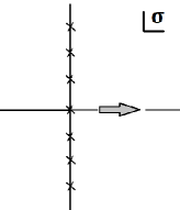
                 $\Leftrightarrow$                 

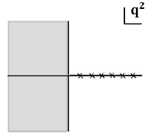
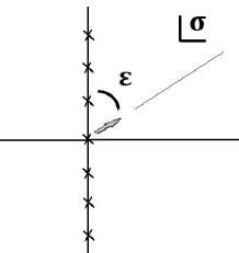
                  $\Leftrightarrow$                 

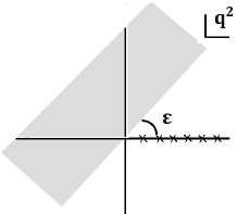
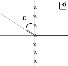
                  $\Leftrightarrow$                 

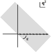
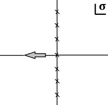
                  $\Leftrightarrow$                 

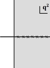
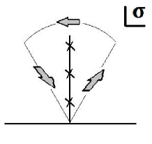
Figure 1: Analytic extension using the generalized Borel-Laplace transform, $\mathcal{B}^{[\rho]}(\sigma)$, in the large-$N_{c}$ limit. Crosses denote poles or branch points in the $\sigma$ plane and the associated poles in the spectrum in the $q^{2}$ plane.

The integral (2) has the form of a Borel-Laplace transform and is defined for $\sigma$ along the positive real axis and for $\frac{\pi}{2}<\arg q^{2}<\frac{3\pi}{2}$, i.e., for $\mathrm{Re}\,q^{2}<0$. However, this definition can be generalized by considering different rays (all starting at the origin) in the complex $\sigma$ plane defined by varying the angle $\arg\sigma$, as long as $\frac{\pi}{2}<\arg\sigma+\arg q^{2}<\frac{3\pi}{2}$ so that the integral in Eq. (2) remains well defined. By varying $\arg\sigma$ the generalized Borel-Laplace transform thus defined analytically extends the definition of $\mathcal{A}(q^{2})$ to larger regions in the $q^{2}$ complex plane [17].

With $\arg\sigma=\frac{\pi}{2}-\epsilon\ (\epsilon>0)$, for example, the region in $q^{2}$ covered becomes $\epsilon<\arg q^{2}<\pi+\epsilon$. Note that this region partly overlaps with the the region we started with, $\frac{\pi}{2}<\arg q^{2}<\frac{3\pi}{2}$, as an analytic continuation should do. If no singularities in the $\sigma$ plane are crossed as $\arg\sigma$ rotates from $0$ to $\frac{\pi}{2}-\epsilon$, and if the function $\sigma\,\mathcal{B}^{[\rho]}(\sigma)$ does not grow exponentially on the contour at infinity connecting these two angles, the result of the two integrals will be the same in the region of overlap. In order for this analytic continuation to work, we have to assume that $e^{\sigma q^{2}}\sigma\,\mathcal{B}^{[\rho]}(\sigma)$ decays to zero at the circle at infinity for $|q^{2}|$ arbitrarily large. We believe that this assumption is satisfied by the representations for $\mathcal{B}^{[\rho]}(\sigma)$ considered in this paper.

To analytically extend the Borel-Laplace integral (2) to the Minkowski axis, it is thus essential to know the location and nature of the singularities of the function $\sigma\,\mathcal{B}^{[\rho]}(\sigma)$ in the complex $\sigma$ plane. As an example, in Fig. 1 we have depicted the singularities in the $\sigma$ plane we will encounter in the large-$N_{c}$ example of Sec. 3. As $\sigma$ is rotated from the positive to the negative real axis, anticlockwise, for example, the presence of any such singularity will add a contribution to the analytic continuation of $\mathcal{A}(q^{2})$ for $q^{2}>0$. Such extra contributions are the source of the duality-violating contributions to $\mathcal{A}(q^{2})$.

Of course, instead of rotating anticlockwise, we could also choose to rotate clockwise in the complex $\sigma$ plane. If we always choose the anticlockwise rotation, the resulting Adler function would not satisfy the Schwarz reflection property, $\mathcal{A}((q^{2})^{*})=[\mathcal{A}(q^{2})]^{*}$. However, we can enforce this property by limiting the anticlockwise rotation to $q^{2}$ with Im $q^{2}\geq 0$, while, instead, rotating clockwise for values of $q^{2}$ with Im $q^{2}<0$. Thus, for negative values of Im $q^{2}$, the rotation at the heart of our analytic continuation should be changed into a clockwise rotation in order to enforce the reflection property. In the rest of this paper, we will always use the anticlockwise rotation, and obtain the spectral function from the Adler function at $q^{2}+i\epsilon$ with $q^{2}$ real and positive. Generally, $\mathcal{A}(q^{2})$ for Im $q^{2}<0$ can be obtained from our results through the Schwarz reflection relation.

It is clear from Eq. (2.7) that the singularity structure of $\sigma\mathcal{B}^{[\rho]}(\sigma)$ is directly determined by the spectrum and that, with present technology, it is not possible to calculate this singularity structure from first principles in the case of QCD. However, there are important qualitative aspects of the spectrum generally assumed to be properties of QCD and, as we will see, these are sufficient to infer with some confidence what type of singularities in $\sigma\mathcal{B}^{[\rho]}(\sigma)$ one may expect. Furthermore, these general observations can be backed up with explicit calculations in model examples, as we will demonstrate below. In the next section, we will consider a concrete example, in order to illustrate the mechanism described qualitatively above. This concrete example will then serve as a starting point for a much more general discussion in Sec. 4, in which we will make contact between the assumed form of the resonance spectrum and the OPE, before using this form to deduce the functional dependence of DVs on $q^{2}$.

3 Example: A simple Regge model for $N_{c}=\infty$

To simplify the discussion, we first consider the large-$N_{c}$ limit, leaving the generalization to finite $N_{c}$ to Secs. 5 and 6. In this limit, we know that the full set of singularities of $\Pi(q^{2})$ in the complex $q^{2}$ plane consists of an infinite sequence of simple poles located at ever increasing values of $q^{2}$ on the positive real $q^{2}$ axis. The spectral function is the corresponding sum of Dirac $\delta$ function contributions. As $\sigma$ is rotated from $\arg\sigma=0$ to $\arg\sigma=\pi/2+\epsilon$ the region of validity in $q^{2}$ of the representation (2) shifts from $\pi/2<\arg q^{2}<3\pi/2$ to $-\epsilon<\arg q^{2}<\pi-\epsilon$, the latter encompassing all the poles of the spectrum. It is clear that these singularities prevent one from performing a naive analytic continuation in $q^{2}$ of the Adler function originally defined for $q^{2}<0$ in Eq. (2). Since $q^{2}$ touches the positive real axis when $\sigma$ touches the positive imaginary axis, some singularities must exist for $\arg\sigma=\pi/2$ which reflect the singularities for $\arg q^{2}=0$.

To see in detail what is going on, we now consider the example of a model in which the spectral function is given by an infinite set of delta functions on a linear trajectory, i.e.,

$$\rho(t)=\sum_{n=1}^{\infty}F(n)\delta\!\left(t-M^{2}(n)\right)\quad,\quad n=1,2,3,\dots\ ,$$ (3.1)

with

$$M^{2}(n)=\Lambda^{2}n\ ,\qquad F(n)=F^{2}\ .$$ (3.2)

We will use units such that $\Lambda=1$, and rescale the spectral function such that $F=1$. This spectrum is not arbitrary. It corresponds to the leading Regge behavior in an expansion for large $n$, where $n$ is the resonance excitation number. In two-dimensions, this asymptotic Regge behavior represents the actual spectrum of QCD in the large-$N_{c}$ limit [34, 35] and, although to date it has never been proved, asymptotic Regge behavior is generally believed to be true in large$-N_{c}$ QCD also in four dimensions. The string picture [36] and phenomenology [33] also provide some evidence for this behavior.

Using this spectrum, the function $\sigma\mathcal{B}^{[\rho]}(\sigma)$ is easily shown to be

$$\sigma\mathcal{B}^{[\rho]}(\sigma)=\frac{\sigma}{\mathrm{e}^{\sigma}-1}=\sum_{n=0}^{\infty}\frac{B(n)}{n!}\,\sigma^{n}\ ,$$ (3.3)

where $B(0)=1,B(1)=-1/2$ and $B(n>1)=\frac{(-1)^{n+1}2(2n)!}{(2\pi)^{2n}}\,\zeta(2n)$ are the Bernoulli numbers and $\zeta(s)$ is the Riemann $\zeta$-function. The function in Eq. (3.3) has simple poles at $\sigma=\pm 2k\pi i\ (k=1,2,3,\dots)$, with residues $\pm 2k\pi i$ (cf. the crosses in the left panels of Fig. 1; the cross at $\sigma=0$ is removed by the factor $\sigma$).

As we try to extend the definition of $\mathcal{A}(q^{2})$ to real $q^{2}>0$ by rotating $\sigma$, we of course hit these poles at $\arg\sigma=\frac{\pi}{2}$. As before, having increased $\arg\sigma$ from $0$ to $\frac{\pi}{2}-\epsilon$, the region of validity of Eq. (2) has shifted to $\epsilon<\arg q^{2}<\pi+\epsilon$. The poles of the spectrum at $n=1,2,3,\dots$ seen in Eq. (3.1) (Fig. 1, second to top panel, right) now lie just outside this new region. Clearly, there is a correspondence between these singularities and the singularities of the Borel function $\sigma\mathcal{B}^{[\rho]}(\sigma)$. If the correlator had no singularities on the positive real $q^{2}$ axis it would be possible to analytically continue $\mathcal{A}(q^{2})$ to include this axis, i.e., to move from the region $\epsilon\leq\arg q^{2}<\pi+\epsilon$ to the region $-\epsilon<\arg q^{2}\leq\pi-\epsilon$. However, the correlator does have poles on the positive real axis, and this is also reflected in the $\sigma$ plane: as $q^{2}$ crosses the positive real axis, $\sigma$ crosses the positive imaginary axis on which the poles of $\sigma\mathcal{B}^{[\rho]}(\sigma)$ are located (Fig. 1, third to top panel).

Letting $\sigma$ cross the imaginary axis, i.e., going from the second to top to the third to top panels in Fig. 1 and reaching $\arg\sigma=\frac{\pi}{2}+\epsilon$ produces a change in the Borel-Laplace integral because now closing the contour at infinity between the two rays encircles the singularities on the positive imaginary $\sigma$ axis (Fig. 1, single panel at the bottom). No further singularities are encountered, and hence no further contributions generated, as $\arg\sigma$ is rotated from $\frac{\pi}{2}+\epsilon$ to $\pi$ and, with $\Gamma$ the contour depicted at the bottom of Fig. 1, one obtains

$$\frac{d\Pi}{dq^{2}}(q^{2})=\int_{\arg\sigma=\pi}d\sigma\ \mathrm{e}^{\sigma q^{2}}\sigma\mathcal{B}^{[\rho]}(\sigma)+\frac{d\Pi_{\rm DV}}{dq^{2}}(q^{2})\ ,\quad(q^{2}>0)\ ,$$ (3.4)

where the “duality violating” contribution $\frac{d\Pi_{\rm DV}}{dq^{2}}(q^{2})$ has been defined as

$$\frac{d\Pi_{\rm DV}}{dq^{2}}(q^{2})=\int_{\Gamma}d\sigma\ \mathrm{e}^{\sigma q^{2}}\sigma\mathcal{B}^{[\rho]}(\sigma)\ .$$ (3.5)

A straightforward use of Cauchy’s theorem leads to

$$\frac{d\Pi_{\rm DV}}{dq^{2}}(q^{2})=2i\pi\frac{d}{dq^{2}}\sum_{k=1}^{\infty}\mathrm{e}^{i2k\pi q^{2}}=-\pi\frac{d}{dq^{2}}\left(\cot\pi q^{2}+i\right)\ .$$ (3.6)

We remark that this result does not satisfy the Schwarz reflection property. However, it is straightforward to check that if we use Eq. (3.6) to define $\Pi_{\rm DV}$ for Im $q^{2}\geq 0$, but instead carry out a clockwise rotation for the analytic continutation to the half-plane Im $q^{2}<0$, the resulting definition of $\Pi_{\rm DV}$ does satisfy the reflection property.

Integrating Eq. (3.3), one obtains

$$\int_{\arg\sigma=\pi}d\sigma\ \mathrm{e}^{\sigma q^{2}}\sigma\mathcal{B}^{[\rho]}(\sigma)=-\frac{d\psi}{dq^{2}}(q^{2})\ ,$$ (3.7)

where $\psi(q^{2})=d\log{\Gamma(q^{2})/dq^{2}}$ is the digamma function. Integrating Eq. (3.4) with respect to $q^{2}$ one thus finds

$$\Pi(q^{2})=-\psi(q^{2})-\pi\left(\cot\pi q^{2}+i\right)+c\quad,\quad(q^{2}>0)$$ (3.8)

where $c$ is an integration constant which can be fixed by the condition $\mathrm{Im}\,\Pi(0)=0$ to be $i\pi$ plus an undetermined real part. We emphasize the emergence of the cotangent function in the process of analytic continuation; we did not invoke the symmetry property

$$\psi(z)=\psi(-z)-\pi\cot(\pi z)-\frac{1}{z}\ ,$$ (3.9)

as was done in previous discussions of this model [3, 5, 6]. In other words, the process of analytic continuation allows us to rederive this global property of the $\psi$ function.

Use of the representation

$$-\pi\cot\pi q^{2}=-\frac{1}{q^{2}}-2q^{2}\sum_{n=1}^{\infty}\frac{1}{(q^{2}+n)(q^{2}-n)}\ ,$$ (3.10)

immediately leads to

$$\frac{1}{\pi}\,\mathrm{Im}\,\Pi(q^{2}+i\epsilon)=\sum_{n=1}^{\infty}\delta(q^{2}-n)\ ,\quad(q^{2}>0)\ ,$$ (3.11)

which reproduces the initial spectrum, as it should (cf. Eq. (3.1)). We see that the information about the spectrum is contained in the DV term of Eq. (3.4). We will now also show that the first term in Eq. (3.4) is indeed the analytic continuation to $q^{2}>0$ of the OPE series obtained from Eq. (2), with $q^{2}<0$.

Denoting by $[q^{2n}]\mathcal{A}_{\rm OPE}(q^{2})$ the $(q^{2})^{-n}$ term in the $1/q^{2}$ expansion of $\mathcal{A}(q^{2})$ and using the representation of Eq. (2), one obtains

$$[q^{2n}]\mathcal{A}_{\rm OPE}\left(q^{2}<0\right)=-q^{2}\ \frac{B(n)}{n!}\ \int_{\arg\sigma=0}\!\!\!d\sigma\ \mathrm{e}^{\sigma q^{2}}\sigma^{n}=\frac{B(n)}{(-q^{2})^{n}}\int_{0}^{\infty}\frac{dt}{n!}\ \mathrm{e}^{-t}t^{n}=\frac{B(n)}{(-q^{2})^{n}}\ ,$$ (3.12)

where the change of variables $t=-q^{2}\sigma>0$ has been made. For $q^{2}>0$, instead, the representation to be used is the one of Eq. (3.7), and one obtains

$$[q^{2n}]\mathcal{A}_{\rm OPE}\left(q^{2}>0\right) = -q^{2}\ \frac{B(n)}{n!}\ \int_{\arg\sigma=\pi}\!\!\!\!\!d\sigma\ \mathrm{e}^{\sigma q^{2}}\sigma^{n}\ ,$$

$$= -q^{2}\ \frac{B(n)}{n!}\ \int_{0}^{-\infty}\!\!\!\!\!d\sigma\ \mathrm{e}^{\sigma q^{2}}\sigma^{n}=\frac{B(n)}{(-q^{2})^{n}n!}\int_{0}^{\infty}\!\!dt\,\mathrm{e}^{-t}\,t^{n}=\frac{B(n)}{(-q^{2})^{n}}\ .$$

Clearly the two results are the same. The factorial behavior of $B(n)$ implies that the expansion is asymptotic.

We end this section with two comments. The first is that, even in the Euclidean regime, Re $q^{2}<0$, the series (3.12) is asymptotic. This is a consequence of the fact that the Borel transform, $\sigma\mathcal{B}^{[\rho]}(\sigma)$, has a finite radius of convergence equal to $2\pi$, the distance of the singularity closest to the origin in the Borel plane. The OPE is obtained by expanding $\sigma\mathcal{B}^{[\rho]}(\sigma)$ around $\sigma=0$ and inserting this expansion into Eq (2). Since the series in $\sigma$ does not converge in the full integration interval, this yields an asymptotic series for the OPE as $-q^{2}\to\infty$. If one cuts off the integral at $\sigma=2\pi$, it is straightforward to show that, at any finite order in the OPE, the remainder is of order $\mbox{exp}(-2\pi|q^{2}|)$ [5]. We see that, in this model, the presence of the singularities at $\sigma=\pm 2\pi i$ has two consequences. First, it affects the nature of the OPE for $q^{2}<0$, where the integral in Eq. (2) is well defined, and, second, it affects the analytic continuation to the Minkowski regime, leading to the DV contribution to the Adler function shown in Eq. (3.4).

The second comment is that no logarithmic terms are present in the asymptotic expansion of the simple model (3.1). As we will see in the following sections, such terms arise only if large-$n$ subleading corrections are added to the model. This simple example, however, demonstrates how the properties of the spectrum are reflected in the singularities of the function $\sigma\mathcal{B}^{[\rho]}(\sigma)$, which, in turn, determine the form of the DVs. We note that the singularities in $\sigma\mathcal{B}^{[\rho]}(\sigma)$ which correspond to the duality violating part of $\Pi(q^{2})$ lie on the imaginary $\sigma$ axis. We will argue in the next section that with subasymptotic corrections to Regge behavior, but still in the large-$N_{c}$ limit, these singularities will stay on the imaginary axis, though they will no longer be simple poles. It then follows that, if large-$N_{c}$ is a good approximation, they will have to stay close to the imaginary axis for finite $N_{c}$, and thus will remain well separated from the cuts in the $\sigma$ plane along the negative real axis which correspond to the perturbative corrections to the OPE.

4 A generalized Regge spectrum for large-$N_{c}$ QCD

In the previous section we saw the consequences of assuming a linear trajectory for the spectrum. In this approximation, $\sigma\mathcal{B}^{[\rho]}(\sigma)$ has simple poles on the positive imaginary axis and the OPE it generates contains no logarithms, but only powers of $1/q^{2}$. How does the picture change when terms which are subleading at large resonance excitation number $n$ are also taken into account? As we will now see, subleading terms change the nature of the singularities from simple poles to branch points, without modifying their location, and introduce logarithmic corrections into the series in powers of $1/q^{2}$.

In general, the function $\mathcal{B}^{[\rho]}(\sigma)$, for Re$\,\sigma>0$, is given in large-$N_{c}$ QCD by a series of the form

$$\mathcal{B}^{[\rho]}(\sigma)=\sum_{n=1}^{\infty}F(n)\,\mathrm{e}^{-\sigma M^{2}(n)}\ ,$$ (4.1)

where the $F(n)$ can in general be complex numbers and $\{M^{2}(n)\}$ is a monotonically increasing sequence of non-negative real numbers tending to infinity (i.e., there is no accumulation point). For the particular case of the vector-current polarization considered here, the quantities $F(n)$ are real and positive. Series like Eq. (4.1) are known as Dirichlet series [37].

The concepts of a radius, boundary and disk of convergence in a power series are replaced for a Dirichlet series by the abscissa, line and half-plane of convergence. The line of convergence is the value $\sigma=\sigma_{c}$ such that for $\mathrm{Re}\,\sigma>\sigma_{c}$ the Dirichlet series converges while for $\mathrm{Re}\,\sigma<\sigma_{c}$ it diverges. The region $\mathrm{Re}\,\sigma>\sigma_{c}$ is called the half-plane of convergence. In our case the line of convergence will be located at Re$\,\sigma=0$, i.e., the imaginary axis. To our knowledge, the first article to point out that Dirichlet series are relevant to the study of large-$N_{c}$ QCD was Ref. [38].

Inspired by two-dimensional QCD, we will assume the spectrum to obey the following expansion at large $n$ [39]:

$$F(n) = 1+\epsilon_{F}(n)\ ,$$ (4.2)

$$M^{2}(n) = n+b\log n+c+\epsilon_{M}(n)\ ,$$

where $b$ and $c$ are constants, and

$$\epsilon_{i}(n) = \epsilon_{i}(0,n)+\epsilon_{i}(\{\lambda\},n)\ ,\quad i=F,M\quad,$$ (4.3)

$$\epsilon_{i}(0,n) = \sum_{\nu_{i}>0}\frac{d^{(i)}(\nu_{i})}{(\log n)^{\nu_{i}}}\ ,$$

$$\epsilon_{i}(\{\lambda\},n) = \sum_{\lambda_{i}>0,\nu_{i}}\frac{d^{(i)}(\lambda_{i},\nu_{i})}{n^{\lambda_{i}}(\log n)^{\nu_{i}}}\ .$$

We take the values of $\lambda_{i}$ in these expressions, and those of the $\nu_{i}$ in $\epsilon_{i}(0,n)$, to be positive, while the values of $\nu_{i}$ in $\epsilon_{i}(\{\lambda\},n)$ are allowed to be positive, negative or zero. The $\epsilon_{i}(n)$ are subleading contributions in the sense that $\epsilon_{F}(n)\rightarrow 0$ and $\epsilon_{M}(n)/n\rightarrow 0$ as $n\to\infty$. The correction $\epsilon_{i}(0,n)$ in Eq. (4.3) is, in fact, just a special case of $\epsilon_{i}(\{\lambda\},n)$ with $\lambda=0$. We choose to split it off because it turns out to generate the logarithms that appear in perturbation theory, whereas the $\epsilon_{i}(\{\lambda\},n)$ corrections with non-zero $\lambda$ contribute to the power corrections. We do not know whether subleading terms of a different form may occur in large-$N_{c}$ QCD, but the forms assumed in Eq. (4.2) turn out to be sufficient for our purpose, which is to further investigate the relation of the detailed structure of the spectrum to the OPE. The behavior $F(n)\to 1$ as $n\to\infty$ (up to an overall multiplicative constant) is a consequence of the asymptotic Regge spectrum $M^{2}(n)\sim n$, as $n\to\infty$, and a requirement to obtain the leading-order parton-model result at large $-q^{2}$.

The rest of this section consists of three parts. First, in Sec. 4.1, we obtain the OPE of the Adler function at large Euclidean momenta from Eq. (4.2). In Sec. 4.2 we focus, in particular, on the first term in the OPE, i.e., perturbation theory. Then, in Sec. 4.3, we generalize the discussion of Sec. 3 and consider the form DVs take in the case of the more general spectrum we assume in this section.

4.1 Expansion for large Euclidean momentum

Let us begin with a study of the singularity structure of the Dirichlet series (4.1) for $\sigma\to 0^{+}$. The expansion around $\sigma=0$ is important because it determines, through Eq. (2), the behavior of the OPE for the Adler function as $-q^{2}\to\infty$. This includes the perturbative series, as the leading term in the OPE.

The mathematical form of the Regge expansion (4.3) is obviously not the most general possible. Therefore, to ensure that limiting our attention to this form is not overly restrictive, it is important to show that, at least in principle, the expansion (4.3) allows us to generate all the inverse powers and logarithms of $q^{2}$ present in the OPE.

In order to proceed, it is useful to recall the identity

$$\mathrm{e}^{-x}=\frac{1}{2i\pi}\int_{C}ds\ x^{-s}\,\Gamma(s)\ ,$$ (4.4)

where $C$ is a vertical line to the right of $\mathrm{Re}\ s=0$ in the complex $s$ plane, i.e., to the right of all singularities of $\Gamma(s)$. One immediately obtains

$$\mathcal{B}^{[\rho]}(\sigma)=\frac{1}{2i\pi}\int_{\widehat{C}}ds\ \sigma^{-s}\,\Gamma(s)\,\Phi(s),\quad\mathrm{where}\quad\Phi(s)=\sum_{n=1}^{\infty}F(n)\left[M^{2}(n)\right]^{-s}\ ,$$ (4.5)

where, as a consequence of the asymptotic behavior in Eq. (4.2), $\Phi(s)$ will have a singularity at $s=1$, implying that now $\widehat{C}$ is a vertical line to the right of $\mathrm{Re}\ s=1$.

As it stands, Eq. (4.5) is exact. A result, known as the Converse Mapping Theorem [40], relates the behavior of $\mathcal{B}^{[\rho]}(\sigma)$ for $\sigma\to 0^{+}$ to the singularities of the function $\Gamma(s)\Phi(s)$. Since the singularities of $\Gamma(s)$ are already known to be simple poles located at non-positive integers, our task is to determine the singularities of $\Phi(s)$.

Let us assume that there is an integer $n^{*}>0$ large enough such that the expansion (4.2) applies for $n>n^{*}$. We can then split

$$\Phi(s)=\Phi_{<}(s)+\Phi_{>}(s)=\sum_{n\leq n^{*}}F(n)\left[M^{2}(n)\right]^{-s}+\sum_{n>n^{*}}^{\infty}F(n)\left[M^{2}(n)\right]^{-s}\ ,$$ (4.6)

and use the expansion (4.2) in the second sum, $\Phi_{>}(s)$. Clearly, the function $\Phi_{<}(s)$ cannot give rise to any singularity in $s$, hence all singularities are contained in $\Phi_{>}(s)$. Let us split

$$\mathcal{B}^{[\rho]}(\sigma)=\mathcal{B}_{<}^{[\rho]}(\sigma)+\mathcal{B}_{\mathrm{>}}^{[\rho]}(\sigma)$$ (4.7)

where $\mathcal{B}_{<}^{[\rho]}(\sigma)$ is the inverse Mellin transform of $\Gamma(s)\Phi_{<}(s)$ and $\mathcal{B}_{\mathrm{>}}^{[\rho]}(\sigma)$ that of $\Gamma(s)\Phi_{>}(s)$. According to the Converse Mapping Theorem, since $\Gamma(s)$ contains simple poles at non-positive integers $s=-k$, $k\geq 0$, the function $\mathcal{B}_{<}^{[\rho]}(\sigma)$ is of the form

$$\mathcal{B}_{<}^{[\rho]}(\sigma)=\sum_{k=0}^{\infty}\frac{(-1)^{k}}{k!}\,\Phi_{<}(-k)\,\sigma^{k}\ ,$$ (4.8)

i.e., it is a power series in $\sigma$. Using Eq. (2), one sees that, at least in principle, one obtains all powers of $1/q^{2}$, as in the OPE. No logarithms appear yet. All logarithms have to come from $\mathcal{B}_{\mathrm{>}}^{[\rho]}(\sigma)$ through the singularities of $\Phi_{>}(s)$, to which we turn next.

Since $\Phi_{>}(s)$ is defined through a sum over $n>n^{*}$, we may insert the expansions in Eq. (4.2) into Eq. (4.5), obtaining

$$\Phi_{>}(s) = \sum_{n>n^{*}}n^{-s}\left(1+b\,\frac{\log n}{n}+\frac{c}{n}+\frac{\epsilon_{M}(n)}{n}\right)^{-s}\left(1+\epsilon_{F}(n)\right)$$

$$= \Phi_{1}(s)+\Phi_{2}(s)\ ,$$

where

$$\Phi_{1}(s) = \sum_{n>n^{*}}n^{-s}\big{(}1+\epsilon_{F}(0,n)\big{)}=\sum_{n>n^{*}}n^{-s}\left(1+\sum_{\nu>0}\frac{d^{(F)}(\nu)}{\log^{\nu}n}\right)\ ,$$ (4.10)

$$\Phi_{2}(s) = \sum_{n>n^{*}}n^{-s}\left(\epsilon_{F}(\{\lambda\},n)-\,\frac{s}{1!}\left(b\frac{\log n}{n}+\frac{c}{n}+\frac{\epsilon_{M}(n)}{n}\right)\right.$$

$$\left.\hskip 85.35826pt+\frac{s(s+1)}{2!}\left(b\frac{\log n}{n}+\frac{c}{n}+\frac{\epsilon_{M}(n)}{n}\right)^{2}+\dots\right)\ .$$

The reason for grouping together in $\Phi_{1}(s)$ the “1” with the terms contained in $\epsilon_{F}(0,n)$ is because these terms will give rise to the logarithms of the perturbative series, whereas the logarithms associated with power corrections will all be contained in $\Phi_{2}(s)$.

Let us first deal with $\Phi_{1}(s)$. One obtains

$$\Phi_{1}(s) = \zeta_{>}(s)+\sum_{\nu>0}d^{F}(\nu)\int_{0}^{\infty}dt\ \frac{t^{\nu-1}}{\Gamma(\nu)}\ \zeta_{>}(s+t)$$

$$\asymp \frac{1}{s-1}+\sum_{\nu>0}d^{F}(\nu)\int_{0}^{\infty}dt\ \frac{t^{\nu-1}}{\Gamma(\nu)}\ \frac{1}{s+t-1}\ ,$$

where $\asymp$ means “singular part of,” and where $\zeta_{>}(s)=\sum_{n>n^{*}}^{\infty}n^{-s}$ has the same singularity structure as the Riemann $\zeta$-function $\zeta(s)$, whose singular expansion is $\zeta(s)\asymp\frac{1}{s-1}$. We substitute Eq. (4.1) into Eq. (4.5), to obtain the $\sigma\to 0^{+}$ expansion of the $\Phi_{1}$ part of $\sigma\mathcal{B}_{\mathrm{>}}^{[\rho]}(\sigma)$. Interchanging the $s$ and $t$ integrals yields

$$\sigma\mathcal{B}_{\mathrm{>}}^{[\rho]}(\sigma)|_{\Phi_{1}}=1+\sum_{\nu>0}d^{F}(\nu)\int_{0}^{\infty}dt\ \frac{t^{\nu-1}}{\Gamma(\nu)}\ \Gamma(1-t)\,\sigma^{t}\ +\mathcal{O}(\sigma^{1-\epsilon})\ ,$$ (4.12)

with $\epsilon$ a parameter that can be chosen arbitrarily close to zero. These manipulations are formal, as the second $t$ integral in Eq. (4.1) diverges at $t\to\infty$ and the $t$ integral in Eq. (4.12) diverges because of the poles in $\Gamma(1-t)$. In App. A we show that, nonetheless, these manipulations are valid, specializing to the case $\nu=1$. It is then straightforward to see that the same argument applies also for $\nu>1$, and we show this explicitly in App. B.

As we will see in Sec. 4.2, Eq. (4.12) is nothing but the Borel transform of the usual perturbative series in powers of $\alpha_{s}$, in the approximation in which only the first term in the $\beta$-function is kept. In fact, the poles in $\Gamma(1-t)$ are related to the renormalon singularities associated with the asymptotic nature of perturbation theory. The presence of the factor $\sigma^{t}=\mathrm{e}^{t\log\sigma}$ shows that $\mathcal{B}^{[\rho]}(\sigma)$ possesses a cut for $\mathrm{Re}\,\sigma<0$. Using Eq. (2), this expression for $\mathcal{B}_{\mathrm{>}}^{[\rho]}(\sigma)$ yields for the perturbative Adler function

$$\mathcal{A}(q^{2})_{\mathrm{\rm PT}} \approx 1+\sum_{\nu>0}d^{F}(\nu)\int_{0}^{\infty}dt\,\frac{t^{\nu-1}}{\Gamma(\nu)}\,\frac{\pi t}{\sin(\pi t)}\,\frac{1}{(-q^{2})^{t}}$$

$$\approx 1+\sum_{\nu>0}d^{F}(\nu)\sum_{k=0}^{\infty}\frac{a_{k}}{\Gamma(\nu)}\ \frac{\Gamma(\nu+k)}{\left(\log(-q^{2})\right)^{\nu+k}}\ ,$$

where the identity

$$\Gamma(1-t)\Gamma(1+t)=\frac{\pi t}{\sin(\pi t)}$$ (4.14)

has been used, and the coefficients $a_{k}$ are defined by

$$\frac{\pi t}{\sin(\pi t)}=\sum_{k=0}^{\infty}a_{k}\,t^{k}\ ,\quad t\rightarrow 0\ .$$ (4.15)

Let us now turn to $\Phi_{2}(s)$. Its contribution is a linear combination of terms of the form

$$(-1)^{\nu}\frac{d^{\nu}}{ds^{\nu}}\zeta_{>}(s+\lambda)=\sum_{n>n^{*}}\frac{\log^{\nu}n}{n^{s+\lambda}}\ ,$$ (4.16)

for $\lambda>0$ and we first consider the case $\nu\geq 0$ (we will comment on the case $\nu<0$ below). Inserting this expression into Eq. (4.5) one obtains, after taking $\lambda$ derivatives with respect to $\sigma$,

$$\frac{d^{\lambda}}{d\sigma^{\lambda}}\mathcal{B}_{\mathrm{>}}^{[\rho]}(\sigma)=^{\circ}(-1)^{\lambda}\ \frac{1}{2i\pi}\int_{\widehat{C}}\ ds\ \sigma^{-s-\lambda}\ \Gamma(s+\lambda)\ (-1)^{\nu}\frac{d^{\nu}}{ds^{\nu}}\zeta_{>}(s+\lambda)\ ,$$ (4.17)

where the symbol $=^{\circ}$ indicates that the right-hand side is just one of the tems in $\frac{d^{\lambda}}{d\sigma^{\lambda}}\mathcal{B}_{\mathrm{>}}^{[\rho]}(\sigma)$. Since

$$(-1)^{\nu}\frac{d^{\nu}}{ds^{\nu}}\zeta_{>}(s+\lambda)\ \asymp\ (-1)^{\nu}\frac{\Gamma(\nu+1)}{(s+\lambda-1)^{\nu+1}}$$ (4.18)

one obtains, after using the residue theorem and integrating $\lambda$ times over $\sigma$,

$$\mathcal{B}_{\mathrm{>}}^{[\rho]}(\sigma)=^{\circ}\ -\ \frac{(-1)^{\lambda}}{\nu+1}\ \frac{\sigma^{\lambda-1}}{\Gamma(\lambda)}\ (-\log\sigma)^{\nu+1}\left(1+\mathcal{O}\left(\frac{1}{\log\sigma}\right)\right)+\mathcal{P}_{\lambda}(\sigma)\ ,$$ (4.19)

where $\mathcal{P}_{\lambda}(\sigma)$ is a polynomial of degree $\lambda$. Substituting this expression into Eq. (2), the contribution to the Adler function is given by

$$\mathcal{A}(q^{2})=^{\circ}-\ \frac{\lambda}{\nu+1}\ \frac{\log^{\nu+1}(-q^{2})}{(q^{2})^{\lambda}}\ \left(1+\mathcal{O}\left(\frac{1}{\log(-q^{2})}\right)\right)+\mathcal{P}_{\lambda+1}\left(\frac{1}{q^{2}}\right)\ .$$ (4.20)

As shown in App. B, it turns out that the result for $\nu<0$ may be obtained from (4.19, 4.20) by analytic continuation in $\nu$, except for the case $\nu=-1$ which, due to the singularity at that value, is a special case. For $\nu=-1$, one obtains (see App. B)

$$\mathcal{B}_{\mathrm{>}}^{[\rho]}(\sigma)=^{\circ}\frac{(-1)^{\lambda-1}}{\Gamma(\lambda)}\,\sigma^{\lambda-1}\,\log(-\log\sigma)\left(1+\mathcal{O}\left(\frac{1}{\log(-\log\sigma)\log\sigma}\right)\right)+\mathcal{P}_{\lambda}(\sigma)\ ,$$ (4.21)

and using Eq. (2),

$$\mathcal{A}(q^{2})=^{\circ}-\ \frac{\lambda}{(q^{2})^{\lambda}}\ \log\log(-q^{2})\left(1+\mathcal{O}\left(\frac{1}{\log(-q^{2})\ \log\log(-q^{2})}\right)\right)+\mathcal{P}_{\lambda+1}\left(\frac{1}{q^{2}}\right)\ .$$ (4.22)

This concludes our exploration of the structure of the OPE generated by the Regge expansion (4.3). Given the variety of logarithmic corrections obtained, and given the adjustable parameters $b$, $c$, and $d^{(i)}(\lambda_{i},\nu_{i})$ in Eq. (4.3), we conclude that the expansion (4.3) is indeed potentially capable of producing all the necessary terms in the OPE, including logarithmic corrections, again in the approximation in which we keep only the leading term in the $\beta$-function. This is confirmed by the work of Ref. [15], which considered this matching between the spectrum and the OPE in more detail using a more direct method, and found that the terms in both the perturbative and $1/q^{2}$ series of the OPE can be matched using the spectrum of Eq. (4.2). We consider these results good evidence for the conjecture that, by adjusting the form of the subleading corrections for $n\to\infty$ in Eqs. (4.2) and (4.3), the complete structure of the OPE, as a function of Euclidean $q^{2}$, can indeed be obtained.

4.2 The perturbative series

We start with a brief review of the standard Borel summation of the divergent perturbative series in QCD. Defining the Borel transform of the perturbative expansion in $\alpha_{s}$ appearing in Eq. (2.4) by

$$B_{\rm PT}^{[{\mathcal{A}}]}(u)=\sum_{n=0}^{\infty}b_{n}u^{n}\ ,\qquad b_{n}=\frac{c_{n+1}}{\beta_{0}^{n+1}\,n!}\ ,$$ (4.23)

the perturbative series is formally summed by the Borel-Laplace integral

$${\mathcal{A}}_{\rm PT}(q^{2})=1+\int\limits_{0}^{\infty}du\,\mathrm{e}^{-u/(\beta_{0}\alpha_{s}(-q^{2}))}\,B_{\rm PT}^{[{\mathcal{A}}]}(u)\ .$$ (4.24)

From renormalon calculus (i.e., the calculation of Feynman diagrams with bubble insertions) one generically expects $c_{n+1}\sim\Gamma(n+1)=n!$ [26]. Therefore, because of the $n!$ in the denominator of $b_{n}$, the series (4.23) is expected to be convergent in a disk $|u|<u_{0}$ with $u_{0}>0$ in the Borel plane. If the integral in Eq. (4.24) would be well defined, the original perturbative series (2.4) would be Borel summable.

Criteria for Borel summability have been formulated in terms of constraints on the expanded function ${\mathcal{A}}_{\rm PT}(q^{2})$ in the complex $\alpha_{s}$ plane [41], but these conditions are not fulfilled in QCD [20]. Borel non-summability is also manifest because the Borel transform $B_{\rm PT}^{[{\mathcal{A}}]}(u)$ has singularities along the positive real axis for $u\geq 2$, the infrared renormalons of Refs. [20, 24, 31], which make the integral (4.24) ambiguous. Other singularities, the ultraviolet renormalons, are located on the negative real axis for $u\leq-1$, and restrict the convergence of the series (4.23) to the disk $|u|<1$.

It is well-known that, in the large-$\beta_{0}$ approximation, in which the coupling is given by Eq. (2.5), there is a simple relation between the standard perturbative Borel transform $B_{\rm PT}^{[{\mathcal{A}}]}(u)$ of the Adler function and the Borel transform of the associated spectral function. This can be easily derived starting from the definition (2.3) of $\rho(t)$ and using the Schwarz reflection property, which allows us to write

$$\rho(t)=\frac{1}{2\pi i}[\Pi(t+i\epsilon)-\Pi(t-i\epsilon)]=\frac{1}{2\pi i}\int_{C_{t}}dq^{2}\,\Pi^{\prime}(q^{2})\ ,$$ (4.25)

where $\Pi^{\prime}(q^{2})$ is the derivative of $\Pi$ and $C_{t}$ is an open contour in the complex plane, with end points $t-i\epsilon$ and $t+i\epsilon$, which does not cross the cut of $\Pi(q^{2})$. Choosing the contour as a circle of radius $t$ centered at the origin, parametrized as $q^{2}=te^{i\phi}$ for fixed $t$ and $0\leq\phi\leq 2\pi$, and using the definition (2.1), we obtain

$$\rho(t)=\frac{1}{2\pi}\int_{0}^{2\pi}d\phi\,{\mathcal{A}}(te^{i\phi})\ .$$ (4.26)

Substituting the Borel-Laplace representation (4.24) with the one-loop coupling (2.5) into this equation and performing the integral over $\phi$ then yields

$$\rho_{\rm PT}(t)=1+\int\limits_{0}^{\infty}du\,\mathrm{e}^{-u\log(t/\Lambda^{2})}\,B_{\rm PT}^{[{\mathcal{A}}]}(u)\,\frac{\sin\pi u}{\pi u}\ .$$ (4.27)

Writing a Borel-Laplace representation for the perturbative spectral function itself,

$$\rho_{\rm PT}(t)=1+\int\limits_{0}^{\infty}du\,\mathrm{e}^{-u/(\beta_{0}\alpha_{s}(t))}\,B_{\rm PT}^{[\rho]}(u)\ ,$$ (4.28)

we recover the relation

$$B_{\rm PT}^{[\rho]}(u)=B_{\rm PT}^{[{\mathcal{A}}]}(u)\,\frac{\sin\pi u}{\pi u}\ ,$$ (4.29)

first derived in Ref. [42].

For the following discussion, it is useful to establish a relation between the standard Borel transform introduced in Eq. (4.29) and the new Borel transform $\mathcal{B}_{\mathrm{>}}^{[\rho]}(\sigma)|_{\Phi_{1}}$ defined in Eq. (4.12). Indeed, by substituting Eq. (4.28) into Eq. (2.7) and performing the integral over $t$ one finds

$$\sigma\mathcal{B}^{[\rho]}_{\rm PT}(\sigma)=1+\int_{0}^{\infty}du\,B_{\rm PT}^{[{\rho}]}(u)\ \Gamma(1-u)\ (\sigma\Lambda^{2})^{u}\ ,$$ (4.30)

where the subscript PT reminds us of the fact that this relation holds in perturbation theory. As we will see, the expression (4.30) is nothing but $\sigma\mathcal{B}_{\mathrm{>}}^{[\rho]}(\sigma)|_{\Phi_{1}}$ defined in Eq. (4.12).

Our discussion in the previous subsection illustrates clearly how the OPE corresponds to the branch-point singularity at $\sigma=0$ in the Borel plane. The purpose of this subsection is to illustrate in more detail how, in terms of the Borel transform of the perturbative series reviewed above, the perturbative series appears in our representation (2) if a general Regge expansion of the form (4.2) is assumed for the spectral function. We again restrict ourselves to the simplified case in which only the first coefficient of the $\beta$-function does not vanish.

Let us recall the expansion for the Borel function $\sigma\mathcal{B}^{[\rho]}(\sigma)$ as $\sigma\to 0^{+}$ in Eq. (4.12):

$$\sigma\mathcal{B}_{\mathrm{>}}^{[\rho]}(\sigma)|_{\Phi_{1}}=1+\sum_{\nu}d^{(F)}(\nu)\int_{0}^{\infty}\!\!\!du\,\frac{u^{\nu-1}}{\Gamma(\nu)}\,\Gamma(1-u)\,\sigma^{u}\ .$$ (4.31)

This is the part which contains the perturbative series. To see this, let us define the combination

$$B^{[\rho]}_{\rm PT}(u)=\sum_{\nu=1}^{\infty}\frac{d^{(F)}(\nu)}{\Gamma(\nu)}\ u^{\nu-1}\ ,$$ (4.32)

so that

$$\sigma\mathcal{B}_{\mathrm{>}}^{[\rho]}(\sigma)|_{\Phi_{1}}=1+\int_{0}^{\infty}du\ B^{[\rho]}_{\rm PT}(u)\ \Gamma(1-u)\,\sigma^{u}\ ,$$ (4.33)

where this expression is to be understood as an asymptotic expansion in $1/\log\sigma$, i.e., as the result of expanding the product $B^{[\rho]}_{\rm PT}(u)\Gamma(1-u)$ in $u$ about $u=0$ and integrating term by term. A comparison of Eq. (4.33) with Eq. (4.30), taking into account that we have taken the QCD scale $\Lambda=1$ in (4.33), establishes the equality of the two expressions, as promised above.

The result (4.24) can be obtained by substituting Eqs. (4.33) and (4.29) into Eq. (2), and, as discussed in the introduction, is valid for $\frac{\pi}{2}<\arg q^{2}<\frac{3\pi}{2}$, i.e., for $\mathrm{Re}\,q^{2}<0$, which includes the Euclidean regime. As we rotate $\sigma$ anticlockwise and reach $\arg\sigma=\pi-\epsilon$, the integral representation (2) analytically continues $\mathcal{A}(q^{2})$ to the region $-\frac{\pi}{2}+\epsilon<\arg q^{2}<\frac{\pi}{2}+\epsilon$. Order by order, this continues $\mathcal{A}(q^{2})$ through the perturbative cut at $q^{2}>0$ into the zeroth Riemann sheet since the function $\mathcal{B}_{\mathrm{>}}^{[\rho]}(\sigma)$ in Eq. (4.33) is continuous, order by order, under the corresponding rotation in $\sigma$. The cut discontinuity of $\mathcal{B}_{\mathrm{>}}^{[\rho]}(\sigma)$ is located further away, at $\arg\sigma=\pi$.

Using the ray $\sigma=|\sigma|\mathrm{e}^{i(\pi-\epsilon)}$, and taking the limit $\epsilon\to 0$, we can thus define the perturbative version of the function $\mathcal{A}(q^{2})$ also for $q^{2}>0$ as

$$\mathcal{A}_{\rm PT}(q^{2}) = 1+q^{2}\int_{0}^{\infty}d|\sigma|\ \mathrm{e}^{-|\sigma|q^{2}}\int_{0}^{\infty}du\ B^{[\mathcal{\rho}]}_{\rm PT}(u)\ \Gamma(1-u)\ |\sigma|^{u}\ \mathrm{e}^{iu\pi}$$

$$= 1+\int_{0}^{\infty}du\ B^{[\mathcal{\rho}]}_{\rm PT}(u)\ \Gamma(1+u)\Gamma(1-u)\ \frac{\mathrm{e}^{iu\pi}}{(q^{2})^{u}}$$

$$= 1+\int_{0}^{\infty}du\ B^{[\mathcal{\mathcal{A}}]}_{\rm PT}(u)\ \mathrm{e}^{-u\left(\log q^{2}-i\pi\right)}\ ,$$

which is nothing else than the well-known result for the analytic continuation to $q^{2}>0$ of $\log(-q^{2})=\log q^{2}-i\pi$ in the Adler function (4.24). This exercise illustrates that the rotation in the complex $\sigma$ plane, supplemented with the right analyticity properties of the function $\mathcal{B}^{[\rho]}(\sigma)$, produces the right analytic continuation in perturbation theory of the Adler function in the $q^{2}$ complex plane.

We would like to close this section with a comment on the so-called “practical version” of the SVZ sum rules [32], obtained by neglecting all logarithmic corrections to the condensates, in the specific case of the vector-channel polarization considered here. We saw in Eq. (2) that the function $\mathcal{B}^{[\rho]}(\sigma)$ is given by

$$\mathcal{B}^{[\rho]}(\sigma)=\int_{0}^{\infty}dt\ \rho(t)\ \mathrm{e}^{-\sigma t}\ ,$$ (4.35)

where $\rho(t)$ is the full spectral function defined in Eq. (2.3). There is of course an analogous mathematical relation between the perturbative counterparts, $\mathcal{B}^{[\rho]}_{\rm PT}(\sigma)$ and $\rho(t)_{\rm PT}$, order by order in powers of $\alpha_{s}$. We then see that the practical version of the SVZ sum rules arises from the assumption that the difference $\mathcal{B}^{[\rho]}(\sigma)-\mathcal{B}^{[\rho]}_{\rm PT}(\sigma)$ is an analytic function of $\sigma$ around the origin, and so can be expanded in a power series in $\sigma$, $\mathcal{B}^{[\rho]}(\sigma)-\mathcal{B}^{[\rho]}_{\rm PT}(\sigma)=\sum_{k=0}^{\infty}c_{k}\ \sigma^{k}$, yielding

$$\sum_{k=0}^{\infty}c_{k}\ \sigma^{k}=\int_{0}^{\infty}dt\ \mathrm{e}^{-\sigma t}\ \Big{(}\rho(t)-\rho(t)_{\rm PT}\Big{)}\ .$$ (4.36)

The left hand side is the Borel-Laplace transform of a series in powers of $1/(-q^{2})$ which is also known as the condensate expansion. In this context, it is traditional to rename the variable $\sigma\to 1/M^{2}$ and rewrite the above equation as [32]

$$\frac{1}{\pi}\int_{0}^{\infty}dt\ \mathrm{e}^{-t/M^{2}}\ \mathrm{Im}\,\Pi(t)=\frac{1}{\pi}\int_{0}^{\infty}dt\ \mathrm{e}^{-t/M^{2}}\ \mathrm{Im}\,\Pi(t)_{\rm PT}+\sum_{k=0}^{\infty}c_{k}\ \frac{1}{M^{2k}}\ ,$$ (4.37)

where $c_{k}$ is related to the condensate of dimension $2k+2$. If we assume that the coefficients $d_{n}$ in Eq. (2.4) are independent of $q^{2}$, we obtain from Eq. (2.1) the “practical version” of the OPE, $\Pi_{\rm OPE}(q^{2})=\sum_{n\geq 1}d_{n}/(n(-q^{2})^{n})$, from which the standard SVZ result, $c_{k}=d_{k+1}/(k+1)!$, immediately follows.

The assumption of analyticity of $\mathcal{B}^{[\rho]}(\sigma)-\mathcal{B}^{[\rho]}_{\rm PT}(\sigma)$ at the origin should, however, be treated with some caution. Even though this practical version of the SVZ sum rules has proved very successful phenomenologically, and while the logarithmic corrections to the condensate expansion are screened by at least one power of $\alpha_{s}$, these logarithms do exist and render the difference $\mathcal{B}^{[\rho]}(\sigma)-\mathcal{B}^{[\rho]}_{\rm PT}(\sigma)$ not analytic in a region around $\sigma=0$. The phenomenological approximation of neglecting such logarithmic corrections to the condensate expansion is not guaranteed to work in general, and should be judged on a case-by-case basis.

4.3 Beyond the OPE

We now turn to the singularities of $\sigma\mathcal{B}^{[\rho]}(\sigma)$ away from the origin. We saw in Sec. 3 that, when the asymptotic Regge behavior is exact, i.e., $M^{2}(n)=n$, $F(n)=1$, the singularities are simple poles located at $\sigma=\pm 2\pi ik$, $k=1,2,3,\dots$. What is the fate of these singularities once the corrections to the spectrum are switched on and the parameters $b,\,c,\,\epsilon_{F,M}(n)$ in Eq. (4.2) become non-zero? To study this question, we focus on the region near the original pole locations. Substituting $\sigma=\widehat{\sigma}+(\sigma-\widehat{\sigma})$ into Eq. (4.1), implementing the expansions (4.2) and (4.3), and taking $\widehat{\sigma}=2\pi ik$, with $k$ a non-zero integer, we find

$$\mathcal{B}_{\mathrm{>}}^{[\rho]}(\sigma)=\frac{1}{2i\pi}\int_{\widehat{C}}ds\ (\sigma-\widehat{\sigma})^{-s}\ \Gamma(s)\Psi_{>}(s)$$ (4.38)

with

$$\Psi_{>}(s)=\mathrm{e}^{-\widehat{\sigma}c}\ \sum_{n>n^{*}}^{\infty}n^{-(s+\widehat{\sigma}\,b)}\left(1-s\left(b\frac{\log n}{n}+\frac{c}{n}\right)+\epsilon_{F}(n)-\left(\frac{s}{n}+\widehat{\sigma}\right)\,\epsilon_{M}(n)+\dots\right)\ ,$$ (4.39)

where we have used that $\mathrm{e}^{-2\pi ikn}=1$. Following steps exactly analogous to those followed before, we find

$$\Psi_{>}(s)\asymp\mathrm{e}^{-\widehat{\sigma}\,c}\,\frac{1}{s+\widehat{\sigma}b-1}+\dots\ ,$$ (4.40)

which translates into

$$\mathcal{B}_{\mathrm{>}}^{[\rho]}(\sigma)=\mathrm{e}^{-\widehat{\sigma}c}\,\frac{\Gamma(1-\widehat{\sigma}b)}{(\sigma-\widehat{\sigma})^{1-\widehat{\sigma}b}}+\dots\ .$$ (4.41)

The form of this result can be understood by considering the poly-logarithm representation of the Dirichlet series in the limit that the $\epsilon_{F,M}(n)$ corrections are neglected. In that limit, one has

$$\sum_{n=1}^{\infty}\mathrm{e}^{-\sigma\left(n+b\log n+c\right)}=\mathrm{e}^{-\sigma c}\sum_{n=1}^{\infty}\frac{\mathrm{e}^{-\sigma n}}{n^{\sigma b}}=\mathrm{e}^{-\sigma c}\,\mathrm{Li}_{\sigma b}(\mathrm{e}^{-\sigma})\ .$$ (4.42)

Since

$$\mathrm{Li}_{\sigma b}(\mathrm{e}^{-\sigma})=\Gamma(1-\sigma b)\sum_{k=-\infty}^{k=+\infty}\frac{1}{\left(\sigma-2\pi ik\right)^{1-\sigma b}}\ ,$$ (4.43)

we see that Eq. (4.41) corresponds precisely to the $k$-th term in this sum, reflecting the fact that (4.41) was obtained by expanding $\mathcal{B}_{\mathrm{>}}^{[\rho]}(\sigma)$ in the neighborhood of $\sigma=\widehat{\sigma}=2\pi ik$.

Equation (4.41) shows that the simple pole at $\widehat{\sigma}=2\pi ik$, present in the exact Regge limit, with $b=0$, as discussed in Sec. 3, has now become a branch point at the same location.

As we show in App. C, the form of the duality-violating contribution to the vector-channel polarization now changes from that given in Eq. (3.6) to

$$\Pi_{\rm DV}(q^{2})=2\pi i\ \sum_{k=1}^{\infty}\mathrm{e}^{i\pi\widehat{\sigma}b}\ (-q^{2})^{-\widehat{\sigma}b}\ \mathrm{e}^{\widehat{\sigma}\left(q^{2}-c\right)}+\dots\ ,$$ (4.44)

where $\widehat{\sigma}=2\pi ik$ and $q^{2}>0$. In Eq. (4.44) only the singularities on the positive imaginary axis contribute, because we rotate anticlockwise in the $\sigma$ plane, so that the sum is restricted to $k>0$. Since

$$(-q^{2})^{-\widehat{\sigma}b}=(-q^{2})^{-2\pi ikb}=\mathrm{e}^{-2\pi ikb\log(-q^{2}-i\varepsilon)}=\mathrm{e}^{-2k\pi^{2}b}\ \mathrm{e}^{-2\pi ikb\log|q^{2}|}\ ,$$ (4.45)

we find that

$$\Pi_{\rm DV}(q^{2})=2\pi i\sum_{k=1}^{\infty}\mathrm{e}^{-4k\pi^{2}b}\,\mathrm{e}^{2\pi ik\left(q^{2}-b\log q^{2}-c\right)}\left(1+\mathcal{O}\left(\frac{1}{\log q^{2}}\right)\right)\ .$$ (4.46)

In Eq. (4.46) we have replaced the dots in Eqs. (4.40) to (4.44) by an explicit estimate of the subleading behavior for large $q^{2}$. We see how the change from simple poles to branch cuts, originating from the logarithmic correction to the spectrum in Eq. (4.2), leads to logarithmic corrections to the exponent appearing in the intermediate step of Eq. (3.6). The result (4.46) still corresponds to the limit $N_{c}\to\infty$, but corrections to a pure Regge spectrum have now been taken into account. If we ignore the $\mathcal{O}(1/\log{q^{2}})$ corrections, and set $b=c=0$, we recover the result of Eq. (3.6). We may again enforce the Schwarz reflection property by defining $\Pi_{\rm DV}(q^{2})$ for Im $q^{2}<0$ by $\Pi_{\rm DV}((q^{2})^{*})=\Pi^{*}_{\rm DV}(q^{2})$.

Rather than discuss this particular result in more detail, we now proceed to a discussion of how this result gets modified when $N_{c}$ is taken large, but finite. We emphasize again the main message, which is that the simple poles on the imaginary axis in the Borel plane found in Sec. 3 stay in the same location, but become branch points instead of simple poles when the spectrum is generalized to be that of Eq. (4.2).

5 DVs for $N_{c}$ large but finite: A warm-up model

In Sec. 4 we have seen how the corrections to the asymptotic Regge spectrum modify the nature, but not the location, of the singularities of the Borel-Laplace transform $\mathcal{B}^{[\rho]}(\sigma)$ in the $N_{c}\to\infty$ limit, and how these singularities determine the form of the DVs. In the following two sections we will discuss how $1/N_{c}$ corrections modify these results when $N_{c}$ is taken large, but finite.

To this end, it is interesting to first study a physically motivated model in which all calculations can be carried out explicitly. The model in question is the one proposed in Ref. [3], and it is defined by the correlator

$$\Pi(q^{2})=\sum_{n=1}^{\infty}\frac{1}{z+n}+constant\ ,$$ (5.1)

where $z=(-q^{2})^{\zeta}$, with $\zeta=1-\mathcal{O}(1/N_{c})<1$. This function has a cut in the complex $q^{2}$ plane for $\arg q^{2}=0$, and poles on the zeroth Riemann sheet that we may associate with resonances. Therefore, the model enjoys the analyticity properties expected in QCD.

In terms of the Borel-Laplace transform, we may write, up to an infinite real constant,

$$\Pi(q^{2})=\int_{0}^{\infty}d\sigma\ \mathrm{e}^{-\sigma z(q^{2})}\ \mathcal{B}^{[\rho]}(\sigma)\ ,\quad\mathrm{Re}\,z>0\ ,$$ (5.2)

where $\mathcal{B}^{[\rho]}(\sigma)$ is given in Eq. (3.3). Since

$$z=|z|\mathrm{e}^{i\psi}=|q^{2}|\mathrm{e}^{i\zeta(\varphi-\pi)}\ ,\quad(0\leq\varphi<2\pi\Leftrightarrow\mathrm{1st\ Riemann\ sheet})\ ,$$ (5.3)

one finds that a full rotation by an angle $\Delta\varphi=2\pi$ in the complex $q^{2}$ plane corresponds to a rotation $\Delta\psi=\zeta\Delta\varphi=2\pi\zeta<2\pi$ in the $z$ plane (recall $\zeta<1$), i.e., there is a deficit angle. The poles of the function (5.1) are located at $\psi=-\pi$ in the $z$ plane, which corresponds to $\varphi=\pi-\pi/\zeta<0$ in the $q^{2}$ plane, i.e., to poles lying on the zeroth Riemann sheet.

Equation (5.2) is defined for $\arg\sigma=0$ and $\mathrm{Re}\,z>0$. As we rotate $\sigma$ anticlockwise, going from $\arg\sigma=0$ to $\arg\sigma=\pi/2-\pi(1-\zeta)=\pi/2-O(1/N_{c})$, we can simultaneously rotate $z$ and $q^{2}$ clockwise, going from $\psi=0$ and $\varphi=\pi$ (i.e., Euclidean $q^{2}$) to $\psi=-\zeta\pi$ and $\varphi=0$ (the Minkowski regime for $q^{2}$). At this point, we have not yet reached the poles of $\mathcal{B}^{[\rho]}(\sigma)$ on the imaginary axis in the $\sigma$ plane. Therefore, this corresponds to a smooth transition in the $q^{2}$ plane from the first to the zeroth Riemann sheet, through the cut at $\varphi=0$.

When we keep rotating $\sigma$, at $\arg\sigma=\pi/2$ we encounter the poles on the imaginary axis of $\mathcal{B}^{[\rho]}(\sigma)$. This corresponds to $\psi=-\pi$ and, through Eq. (5.3), to $\varphi=\pi-\pi/\zeta<0$, i.e., to resonance poles in $q^{2}$ lying on the zeroth Riemann sheet. It is this correspondence between the location of the singularities of $\mathcal{B}^{[\rho]}(\sigma)$ in the $\sigma$ plane and the location of the singularities of $\Pi(q^{2})$ in the $q^{2}$ plane that we wish to again emphasize here. The location of the resonance poles which obstruct the analytic continuation in $q^{2}$ and the location of the singularities in $\mathcal{B}^{[\rho]}(\sigma)$ which obstruct the analytic continuation in $\sigma$ are linked through the Borel-Laplace transform.

If we keep rotating $\sigma$ anticlockwise, crossing the poles on the imaginary axis, we will again pick up the contribution from the residues of those poles, through Cauchy’s theorem, leading to DVs having the form of the cotangent function in Eq. (3.6), with the variable $q^{2}$ replaced by $z$. This is precisely the correct result for DVs in this model [3].

6 DVs for $N_{c}$ large but finite: QCD

Let us now discuss the effect of $1/N_{c}$ corrections in the case of QCD. It is clear that the large-$N_{c}$ limit must be taken with care. As we have seen in Eq. (4.46), in the strict large-$N_{c}$ limit DVs are not a small correction to the (analytically continued) OPE. This is not surprising, since the large-$N_{c}$ limit of the spectral function is not a good approximation to the real-world spectral function.

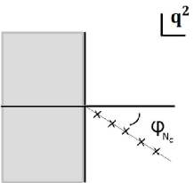
                  $\Leftrightarrow$                 

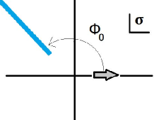
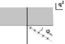
                  $\Leftrightarrow$                 

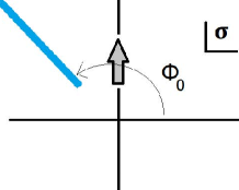
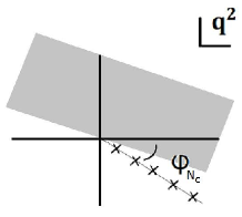
                  $\Leftrightarrow$                 

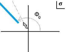
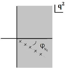
                  $\Leftrightarrow$                 

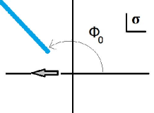
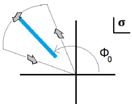
Figure 2: Contour used to jump over the cut in the $\sigma$ plane. Analytic extension into the zeroth Riemann sheet using the generalized Borel-Laplace transform.

The spectrum of QCD is not known in any detail at large, but finite, $N_{c}$, so we can no longer calculate the function $\sigma\mathcal{B}^{[\rho]}(\sigma)$ from Eq. (2.7) as we did in the previous sections. Some important qualitative features of the spectral function are known, however. Moving away from the strict large-$N_{c}$ limit to $N_{c}$ large but finite, it is known, for example, that the poles of $\Pi(q^{2})$ on the Minkowski axis move a small distance away into the zeroth Riemann sheet and a cut in $\mathrm{Im}\,\Pi(q^{2})$ appears on this axis.

Starting from the initial representation (2) with $\arg\sigma=0$, valid for $\frac{\pi}{2}<\arg q^{2}<\frac{3\pi}{2}$, as we rotate towards $\arg\sigma=\frac{\pi}{2}+\epsilon$ and cover the region $-\epsilon<\arg q^{2}<\pi-\epsilon$, now nothing dramatic occurs. In contrast to the case of the strict large-$N_{c}$ limit, where the resonance poles are located on the Minkowski axis, now that $N_{c}$ is finite, as we move from $\arg q^{2}=+\epsilon$ to $\arg q^{2}=-\epsilon$, crossing the Minkowski axis, we move into the zeroth Riemann sheet without encountering any singularity. This is so because $\Pi(q^{2})$, as we saw in the warm-up model model in Sec. 5, and in the perturbative series in Sec. 4.2, is continuous across the corresponding cut. It is only as $\arg q^{2}$ becomes more negative, and $q^{2}$ moves deeper into the zeroth Riemann sheet, that the poles corresponding to the presence of resonances are encountered. When $N_{c}$ is large (but finite) a resonance pole in the complex plane is located at an angle $\varphi_{N_{c}}$ given by

$$\tan\varphi_{N_{c}}\approx\varphi_{N_{c}}=-\frac{\Gamma}{M}=-\frac{a}{N_{c}}\left(1+\mathcal{O}\left(\frac{1}{N_{c}}\right)\right)\ ,$$ (6.1)

where $a\sim N_{c}^{0}>0$ and we have used that $\Gamma\sim 1/N_{c}$ and $M\sim N_{c}^{0}$. A string-based model suggests that the parameter $a$ is independent of the resonance excitation number $n$ [36]. Thus, as $1/N_{c}$ corrections cause the resonance poles to rotate clockwise by an angle $\varphi_{N_{c}}\approx-\frac{a}{N_{c}}$ in the complex $q^{2}$ plane, the singularities of $\mathcal{B}^{[\rho]}(\sigma)$ in the complex $\sigma$ plane, according to Eq. (2), rotate anticlockwise by the same angle past the positive imaginary axis. These singularities must therefore be located (approximately) along the ray $\arg\sigma\simeq\frac{\pi}{2}+\frac{a}{N_{c}}\equiv\phi_{0}$ (see Fig. 2), where we have assumed here that $a$ does indeed not depend on $n$. In fact, we are primarily interested in the singularity closest to the origin, as this will be the one that generates the leading contribution to the DVs. A mild dependence of $a$ on $n$ will thus have no impact on our conclusions.

If the large-$N_{c}$ limit is a reasonably smooth one, the distance of this closest singularity to the origin cannot be too different from that found in the $N_{c}=\infty$ limit in Sec. 4, namely, $|\widehat{\sigma}(k=1)|=|2\pi i|=2\pi$. We thus assume that the singularity closest to the origin is located at $\widehat{\sigma}=\sigma_{0}\ \mathrm{e}^{i\phi_{0}}$ with $\phi_{0}=\frac{a}{N_{c}}+\frac{\pi}{2}$ and $\sigma_{0}=2\pi$, up to subleading $1/N_{c}$ corrections, as depicted in Fig. 2.

In this case, as $\sigma$ is rotated from $\arg\sigma=0$ to $\arg\sigma=\pi$, we cross the branch cut (depicted by a blue line in Fig. 2). This generates a DV contribution given by the integral over the contour, $\Gamma$, shown in the bottom panel of Fig. 2, akin to that appearing in Eq. (3.5) of Sec. 3, and having the form

$$\frac{d\Pi_{\rm DV}}{dq^{2}}(q^{2})=\int_{\Gamma}d\sigma\ \mathrm{e}^{\sigma q^{2}}\sigma\mathcal{B}^{[\rho]}(\sigma)\ ,$$ (6.2)

where we can now take $q^{2}>0$. Equivalently,

$$\Pi_{\rm DV}(q^{2})=\int_{\Gamma}d\sigma\ \mathrm{e}^{\sigma q^{2}}\mathcal{B}^{[\rho]}(\sigma)\ ,$$ (6.3)

up to a constant of integration which, as in Sec. 3, has no physical effect.

Let us assume that the function $\mathcal{B}^{[\rho]}(\sigma)$ is of the general form

$$\mathcal{B}^{[\rho]}(\sigma)=\frac{a_{0}}{(\sigma-\widehat{\sigma})^{1+\gamma}}\left[1+a_{1}\left(\sigma-\widehat{\sigma}\right)^{p_{1}}+\frac{a_{\log}}{\log(\sigma-\widehat{\sigma})}+\dots\right]\ ,$$ (6.4)

where $\gamma=-\widehat{\sigma}b+\mathcal{O}(N_{c}^{-1})$, and $a_{0}=\mathrm{e}^{-\widehat{\sigma}c}\ \Gamma(1+\gamma)\left(1+\mathcal{O}\left(N_{c}^{-1}\right)\right)$, in accordance with Eq. (4.41) in Sec. 4.3. The generic parameters $p_{1}>0$ and $a_{1},\,a_{\log}$ encapsulate the dependence on the corrections to the Regge spectrum associated with the quantities $\epsilon_{F,M}$ in Eq. (4.39). One then obtains for the associated duality-violating contribution

$$\Pi_{\rm DV}(q^{2})=\int_{\sigma_{0}\ \mathrm{e}^{i\phi_{0}}}^{\infty\ \mathrm{e}^{i\phi_{0}}}d\sigma\ \mathrm{e}^{\sigma q^{2}}\mathrm{Disc}\{\mathcal{B}^{[\rho]}(\sigma)\}\ ,$$ (6.5)

which yields (cf. App. C)

$$\Pi_{\rm DV}(q^{2})=2\pi i\ \mathrm{e}^{-2\pi i\left(c+\gamma/2\right)}\,(-q^{2})^{\gamma}\ \mathrm{e}^{q^{2}\widehat{\sigma}}\left[1+a_{1}\,\frac{\Gamma(1+\gamma)}{\Gamma(1+\gamma-p_{1})}\,\frac{\mathrm{e}^{i\pi p_{1}}}{(-q^{2})^{p_{1}}}+\frac{a_{\log}}{\log q^{2}}+\dots\right]\ .$$ (6.6)

This result depends solely on the location of the branch point ($\widehat{\sigma}=\sigma_{0}\ \mathrm{e}^{i\phi_{0}}$) and the nature of the branch cut, $\gamma$. The orientation of the branch cut in the complex plane is irrelevant, as expected.

For $N_{c}$ large, recalling that $\widehat{\sigma}=\sigma_{0}\left(-\sin(\frac{a}{N_{c}})+i\cos(\frac{a}{N_{c}})\right)=2\pi(i-\frac{a}{N_{c}})\left(1+\mathcal{O}(N_{c}^{-1})\right)$ and $\gamma=-2\pi ib+\mathcal{O}(N_{c}^{-1})$, one obtains

$$\Pi_{\rm DV}(q^{2}) = 2\pi i\,\mathrm{e}^{-2\pi^{2}b}\,\mathrm{e}^{-2\pi ci}\,(-q^{2})^{-2\pi ib}\ \mathrm{e}^{2\pi q^{2}\left(i-\frac{a}{N_{c}}\right)}\$$ (6.7)

$$\times\left[1+a_{1}\,\frac{\Gamma(1-2\pi ib)}{\Gamma(1-2\pi ib-p_{1})}\,\frac{\mathrm{e}^{i\pi p_{1}}}{(-q^{2})^{p_{1}}}+\frac{a_{\log}}{\log q^{2}}+\dots\right]+\mathcal{O}\left(\frac{1}{N_{c}}\right)\ ,$$

from which one can extract the leading contribution

$$\Pi_{\rm DV}(q^{2}) \approx \ 2\pi i\,\mathrm{e}^{-4\pi^{2}b}\,\mathrm{e}^{-2\pi q^{2}\frac{a}{N_{c}}}$$

$$\times\bigg{[}\cos 2\pi\Big{(}q^{2}-c-b\log{q^{2}}\Big{)}+i\sin 2\pi\Big{(}q^{2}-c-b\log{q^{2}}\Big{)}\bigg{]}\$$

$$\hskip 56.9055pt\left(1+\mathcal{O}\left(\frac{1}{N_{c}};\frac{1}{(q^{2})^{p_{1}}};\frac{1}{\log q^{2}}\right)\right)\ ,$$

where Eq. (4.45) has again been used. Since Eq. (6) is valid for $q^{2}>0$, taking the imaginary part yields the DV part of the spectral function. As before, Eq. (6.7) also gives $\Pi_{\rm DV}(q^{2})$ in the complex plane, for Re $q^{2}>0$ and Im $q^{2}>0$. For Im $q^{2}<0$ it is defined using $\Pi_{\rm DV}((q^{2})^{*})=[\Pi_{\rm DV}(q^{2})]^{*}$, thus enforcing the reflection property. The new contribution $-q^{2}d\Pi_{\rm DV}(q^{2})/dq^{2}$ should be added to Eq. (2.4) in order to obtain a complete representation of the Adler function in the Minkowski region, for large $q^{2}$.

As one can see, the main effect of the subleading terms in the Regge expansion at large $n$ is the logarithmic correction to the argument of the cosine and sine functions modulating the exponential falloff with $q^{2}$. There are at least two reasons to expect these corrections to generate only small modifications to these sinusoidal factors. First, $|b\log q^{2}|\ll q^{2}$ for any $b$ at large $q^{2}$. Second, the phenomenological knowledge which, as we have said, supports a Regge behavior in QCD, does not yield any evidence for a non-zero value for the $\log n$ term in the mass spectrum. In other words, phenomenology is consistent with a small $b$ in QCD. This result provides theoretical support for the parametrization introduced in [5, 6], which was successfully tested against precise data for the non-strange vector and axial-vector spectral functions obtained from hadronic $\tau$ decays by the OPAL [44] and ALEPH [45] experiments, in a series of analyses of the QCD coupling, $\alpha_{s}$ [11, 12, 13]. In App. D we give some numerical evidence for the agreement between the results obtained from the fits to Regge trajectories obtained, e.g., in Ref. [33], and those obtained from fits to the $\tau$ data. Further theoretical studies using the functional analysis methods developed in [46, 47] may also help understanding the origin and nature of DVs in QCD.

We end this section with two comments. First, as already noted at the end of Sec. 3, even for Euclidean $q^{2}$, the OPE for $\Pi(q^{2})$ is asymptotic, and, at any finite order the remainder is of order $\mbox{exp}(-R|q^{2}|)$, where $R$ is the distance of the nearest non-perturbative singularity in the Borel plane. Here, up to $1/N_{c}$ corrections, $R=2\pi$, and thus these exponential remainders are much smaller than the exponential suppression factor $\mbox{exp}(-2\pi q^{2}a/N_{c})$ in Eq. (6) for $N_{c}$ large enough. This singularity thus plays two roles: the absolute value of its position in the complex plane sets the size of the exponential remainder for the OPE in the Euclidean regime, while both the absolute value and its phase determine the form of the DV contributions in the Minkowski regime. This can be explicitly verified in the simple model of Sec. 3, for example. In the more realistic approach of the subsequent sections, also a logarithmic cut starting at $\sigma=0$ in the Borel plane appears. However, this cut plays a different role, leading to the logarithmic corrections in each term in the OPE, as discussed in Sec. 4.1 above. Second, if we take $q^{2}=s+i\Delta$ in Eq. (6.7), we find that DVs are exponentially suppressed with a factor $\mbox{exp}[-2\pi\Delta]$ away from the positive real $q^{2}$ axis. If we then follow the prescription of Ref. [1] by taking $\Delta\propto s$, DVs are exponentially suppressed at large $s$, even in the limit $N_{c}\to\infty$. Our results are thus consistent with the smearing method proposed in Ref. [1].

7 Conclusions

In this paper, we analyzed the large $q^{2}$ behavior of the Adler function, with the aim of deriving its form on the Minkowski axis, where neither perturbation theory nor its supplemented version, represented by the full OPE, provide a reliable representation. While the OPE is the dominant contribution at large $q^{2}$, there are additional nonperturbative contributions, which are not part of the OPE. These quark-hadron duality violating contributions can be probed starting from fairly general assumptions about the spectrum using the techniques of complex analysis. Our main result is the expression for the leading duality-violating contribution to the vacuum polarization, given in Eq. (6).

For any analysis such as ours, some non-perturbative input going beyond the OPE is needed. This non-perturbative input should reflect the properties of the spectrum, which determines the Adler function through the dispersion relation, Eq. (2). This relation also shows that the Adler function is a function of one variable, $q^{2}$ (as long as we work in the chiral limit), expressed in terms of the scale of QCD. However, in practice, by introducing the perturbative coupling $\alpha_{s}(-q^{2})$, it is usually rearranged in terms of a double expansion in powers of $\alpha_{s}(-q^{2})$ and $1/q^{2}$, given a choice of renormalization scheme.

Our analysis is based on the fact that we can write the Adler function as the Borel transform, in the plane of the complex variable $\sigma$, of a function $\sigma B^{[\rho]}(\sigma)$, where $B^{[\rho]}(\sigma)$ is, itself, the Laplace transform of the spectral function, cf. Eqs. (2) and (2.7). The Borel-Laplace transform $\mathcal{B}^{[\rho]}(\sigma)$ allows us to effectively continue the asymptotic expansion of the OPE from the Euclidean to the Minkowski domain. This is accomplished by taking advantage of the combination of the exact nature of the dispersion relation (2) and the powerful techniques of analytic continuation. The Borel-Laplace representation, moreover, allows us to relate the large Euclidean $q^{2}$ behavior of the Adler function to the behavior of $\mathcal{B}^{[\rho]}(\sigma)$ near $\sigma=0$. In particular, the logarithmic corrections to the OPE are directly related to the cut along the negative real axis emanating from $\sigma=0$ in the Borel plane, as shown in Secs. 4.1 and 4.2. In Sec. 4.2 we also recovered the standard renormalon picture relating the OPE to perturbation theory, and rederived the SVZ sum rules.

There can be no singularities to the right of the imaginary axis in the $\sigma$ plane, as follows directly from Eq. (2). However, we find that, beyond the singularity at $\sigma=0$, there may be further singularities in the half-plane Re $\sigma\leq 0$, with the location and nature of these singularities depending on general properties of the spectrum.

Since the full spectrum of QCD is not known, even in the large-$N_{c}$ and chiral limits, we have had to make assumptions in order to be able to identify the location and nature of these singularities. Our main assumption is that, for asymptotically large energies, the spectrum for $N_{c}=\infty$ lies on a Regge trajectory. This assumption is supported by phenomenology, intuitive arguments based on string theory and the solution of large-$N_{c}$ QCD in two dimensions. At large but finite energies, we parametrize the spectrum in terms of a rather general form, with many parameters ($b$, $c$ and the parameters $d^{(F,M)}(\nu_{F,M})$ and $d^{(F,M)}(\lambda_{F,M},\nu_{F,M})$ of Eqs. (4.2) and (4.3)). Starting from the limit $N_{c}\to\infty$, it turns out to be possible to extend the analysis to large but finite $N_{c}$, with plausible additional assumptions (see Sec. 6).

While we cannot derive these assumptions from QCD, we can show that, starting from these assumptions, it is possible to reconstitute the OPE for large Euclidean $q^{2}$. Explicitly, with the general parametrization of the spectrum given by Eqs. (4.2) and (4.3), there is enough freedom available to allow a match to the usual form of the OPE, where inverse logarithms can be re-expressed in terms of $\alpha_{s}(-q^{2})$ in the large-$\beta_{0}$ approximation. This result can be generalized to include also higher-order terms in the $\beta$ function affecting the relation between $q^{2}$ and $\alpha_{s}(-q^{2})$. In fact, our results agree with those of Ref. [15], where also some contributions beyond the large-$\beta_{0}$ approximation were considered. While we have not traced the contribution of all such needed additional Regge spectrum corrections to our final result, Eq. (6), we conjecture that such corrections will not alter the shape of the leading expression for $\Pi_{\rm DV}(q^{2})$.

We find that for $N_{c}\to\infty$, the singularities of $\mathcal{B}^{[\rho]}(\sigma)$ are located on the imaginary axis, while for finite $N_{c}$ they rotate anticlockwise from the imaginary $\sigma$ axis by an amount $\sim 1/N_{c}$, associated with the decay widths of resonances. The singularity closest to the origin, at a distance approximately equal to $2\pi$ in units of the Regge slope, yields the leading term in the duality-violating contribution to the vacuum polarization, Eq. (6). Singularities farther away lead to exponentially subleading terms. These singularities are unlike the cut starting at $\sigma=0$ along the negative real axis, which is associated with the perturbative expansion (and perturbative corrections to the higher-order terms in the OPE), as discussed in Sec. 4.2. In this sense, the two types of singularities in the Borel plane, and, therefore, the two expansions, are clearly separated.

We conjecture that the existence of these singularities in the Borel plane is more general than just a consequence of the Regge behavior, with corrections of the form assumed in this paper. These singularities in the $\sigma$ plane are a direct consequence of the fact that the spectral function extends all the way to infinity: if the spectral function were to vanish beyond a finite value, $t_{max}$, of $t$, there would be no singularities in $\sigma$, and the OPE would be a convergent power series in $1/q^{2}$ (for $q^{2}>t_{max}$) without any corrections logarithmic in $q^{2}$. Thus, the fact that the OPE is divergent suggests that there are contributions which are exponentially suppressed in the inverse of the expansion variable, $1/q^{2}$, in accordance with the notion of a transseries, and this is precisely what we find to be the case.

There are several questions we have not answered. One obvious question is whether our analysis can be extended systematically beyond the class of corrections to a Regge spectrum given by Eqs. (4.2) and (4.3), and, connected to that, beyond the large-$\beta_{0}$ approximation. Another physically interesting question is how our results would change when a non-vanishing quark mass is taken into account. These questions are beyond the scope of the current paper.

APPENDICES

Appendix A Proof of Eq. (4.12)

Let us take the following Dirichlet series, corresponding to the choice $\nu=1$ in $\Phi_{1}(s)$ in Eq. (4.10):

$$\chi(\sigma)=\sigma\sum_{n>n^{*}}^{\infty}\frac{\mathrm{e}^{-\sigma n}}{\log n}\ ,$$ (A.1)

with $n^{*}\gg 1$. The generalization to powers $\nu>1$ of the logarithm is straightforward (see also App. B below). The function $\chi(\sigma)$ is singular at $\sigma=0$ and we wish to find out what leading the behavior of this function is as $\sigma\to 0^{+}$. We rewrite

$$\chi(\sigma) = \sigma\int_{0}^{\infty}dt\ \sum_{n>n^{*}}^{\infty}\mathrm{e}^{-\sigma n}\mathrm{e}^{-t\log n}=\sigma\int_{0}^{\infty}dt\sum_{n>n^{*}}^{\infty}\mathrm{e}^{-\sigma n}\,n^{-t}$$

$$= \sigma\int_{0}^{\infty}dt\ \frac{1}{2i\pi}\int_{C}ds\,\sigma^{-s}\,\Gamma(s)\sum_{n>n^{*}}^{\infty}n^{-s-t}$$

$$= \sigma\int_{0}^{\infty}dt\ \frac{1}{2i\pi}\int_{C}ds\,\sigma^{-s}\,\Gamma(s)\,\zeta_{>}(s+t)\ ,$$

where we have defined $\zeta_{>}(s+t)=\sum_{n>n^{*}}n^{-s-t}$. The singular expansion of this function is the same as that of $\zeta(s+t)$, namely $\zeta_{>}(s+t)\asymp 1/(s+t-1)$, and this requires $C$ in Eq. (A) to be a vertical straight line with $\mathrm{Re}\,s>1$ . Clearly $\zeta_{>}(z)=\zeta(z)-\zeta_{<}(z)$, where $\zeta_{<}(z)=\sum_{n\leq n^{*}}n^{-z}$ is a regular function of $z$ containing no singularities. One can then split

$$\chi(\sigma)=\chi(\zeta,t_{<};\sigma)-\chi(\zeta_{<},t_{<};\sigma)+\chi(\zeta_{>},t_{>};\sigma)\ ,$$ (A.3)

where

$$\chi(\zeta,t_{<};\sigma) = \frac{1}{2i\pi}\int_{C}ds\ \sigma^{1-s}\ \Gamma(s)\int_{0}^{1-\delta}\ dt\ \zeta(s+t)$$ (A.4)

$$\chi(\zeta_{<},t_{<};\sigma) = \frac{1}{2i\pi}\int_{C}ds\ \sigma^{1-s}\ \Gamma(s)\int_{0}^{1-\delta}\ dt\ \zeta_{<}(s+t)$$

$$\chi(\zeta_{>},t_{>};\sigma) = \frac{1}{2i\pi}\int_{C}ds\ \sigma^{1-s}\ \Gamma(s)\int^{\infty}_{1-\delta}\ dt\ \zeta_{>}(s+t)$$

for a certain parameter $\delta$, with $0<\delta\ll 1$. We can now evaluate or bound each of these integrals in turn.

Since the function $\Gamma(s)$ has poles at non-positive integers and is regular for $s=1-t$ in the interval $0\leq t\leq 1-\delta$, one may use $\zeta(s+t)\asymp 1/(s+t-1)$ and the Converse Mapping Theorem [40] to write

$$\chi(\zeta,t_{<};\sigma) = \int_{0}^{1-\delta}dt\ \sigma^{t}\ \Gamma(1-t)+\sum_{k=0}^{\infty}\frac{(-1)^{k}}{k!}\,\sigma^{1+k}\int_{0}^{1-\delta}dt\ \zeta(t-k)$$

$$= \int_{0}^{1-\delta}dt\ \mathrm{e}^{t\log\sigma}\ \Gamma(1-t)+\mathcal{O}(\sigma)$$

$$= \sum_{k=0}^{\infty}c_{k}\int_{0}^{1-\delta}dt\,t^{k}\,\mathrm{e}^{t\log\sigma}+\mathcal{O}(\sigma)\ ,$$

where the $\Gamma(1-t)$ has been expanded in powers of $t$, with $c_{k}\to 1$ as $k\to\infty$. Next, we split each term in the sum over $k$ into the difference of an integral between $0$ and $\infty$, and an integral between $1-\delta$ and $\infty$, with each of these integrals being convergent (recall that we take $\sigma\to 0^{+}$). This yields an asymptotic expansion for $\chi(\zeta,t_{<};\sigma)$ in powers of $1/\log\sigma$. Using the saddle point method, one finds that

$$\int_{1-\delta}^{\infty}dt\,t^{k}\,\mathrm{e}^{t\log\sigma}\sim\mathcal{O}\left(\frac{\sigma^{1-\delta}}{\log\sigma}\,(1-\delta)^{k}\right)\ ,$$ (A.6)

and we thus arrive at

$$\chi(\zeta,t_{<};\sigma)=c_{0}\,\frac{\Gamma(1)}{(-\log\sigma)}+c_{1}\,\frac{\Gamma(2)}{(-\log\sigma)^{2}}+c_{2}\,\frac{\Gamma(3)}{(-\log\sigma)^{3}}+\dots+\mathcal{O}\left(\sigma,\frac{\sigma^{1-\delta}}{\log\sigma}\right)\ .$$ (A.7)

Notice that $(-\log\sigma)>0$ when $\sigma\to 0^{+}$, so the series (A.7) is not alternating, and thus this expansion is not Borel summable.

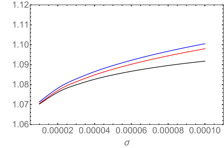
Figure 3: Comparison of the Dirichlet series (A.1) and the result (A.10). Blue curve: the Dirichlet series (A.1) with the sum running over $n$, with $2\leq n<\infty$. Black curve: the same Dirichlet series, but now for $20\leq n<\infty$. Red curve: the result of the asymptotic expansion (A.10) keeping 5 terms in the series. The three functions have been multiplied by $(-\log\sigma)$.

Let us now turn to the function $\chi(\zeta_{<},t_{<};\sigma)$ in Eq. (A.4). The only singularities in the integrand in $s$ are those of $\Gamma(s)$. This leads to a result of $\mathcal{O}(\sigma)$, which is already included in (A.7).

Finally we have to evaluate $\chi(\zeta_{>},t_{>};\sigma)$ in Eq. (A.4). Although originally the contour $C$ in this integral has $\mathrm{Re}\ s>1$, since the rightmost singularity of $\zeta_{>}(s+t)$ is at $s=\delta$ in the interval $1-\delta\leq t<\infty$, one is allowed to shift this contour to the left to $\mathrm{Re}\ s=\delta^{\prime}>\delta$ without changing the result. Then, defining $s=\delta^{\prime}+iu$ one finds

$$\chi(\zeta_{>},t_{>};\sigma)=\frac{\sigma^{1-\delta^{\prime}}}{2\pi}\int_{-\infty}^{\infty}du\ \sigma^{-i\,u}\ \Gamma(\delta^{\prime}+i\,u)\int_{1-\delta}^{\infty}dt\ \zeta_{>}(\delta^{\prime}+i\,u+t)\ .$$ (A.8)

This function is bounded, i.e.,

$$|\chi(\zeta_{>},t_{>};\sigma)| \leq \frac{\sigma^{1-\delta^{\prime}}}{2\pi}\ M(\delta^{\prime},\delta)$$ (A.9)

$$M(\delta,\delta^{\prime}) = \int_{-\infty}^{\infty}du\ \left|\Gamma(\delta^{\prime}+i\,u)\right|\ \int_{1-\delta}^{\infty}dt\ \left|\zeta_{>}(\delta^{\prime}+i\,u+t)\right|\ .$$

The integral for $M(\delta,\delta^{\prime})$ is finite for the allowed region of the parameters $\delta$ and $\delta^{\prime}$. Since we may choose $\delta$, and thus $\delta^{\prime}>\delta$ arbitrarily small, we see that $\chi(\zeta_{>},t_{>};\sigma)$ is exponentially suppressed in comparison with the terms in the series (A.7) for $\sigma\to 0^{+}$.

Putting together all the above results we conclude that

$$\chi(\sigma)=c^{(0)}\frac{\Gamma(1)}{(-\log\sigma)}+c^{(1)}\frac{\Gamma(2)}{(-\log\sigma)^{2}}+c^{(2)}\frac{\Gamma(3)}{(-\log\sigma)^{3}}+\dots+\mathcal{O}\left(\sigma,\sigma^{1-\delta^{\prime}},\frac{\sigma^{1-\delta}}{\log\sigma}\right)\ ,$$ (A.10)

where $\delta>0$ and $\delta^{\prime}>\delta$ can be chosen arbitrarily small.

In Fig. 3 we show a comparison of the original Dirichlet series (A.1) evaluated numerically and the result (A.10), after multiplying by $(-\log\sigma)$. The difference between the blue and the black curves is the starting value of $n$ in the sum (A.1). The agreement as $\sigma\to 0^{+}$ shows that the dependence on $\sigma$ as $\sigma\to 0^{+}$ depends solely on the asymptotic behavior for large $n$ in this sum and not on the first terms for low $n$. As one can see, the result (A.10) reproduces rather well the behavior of $\chi(\sigma)$ as $\sigma\to 0^{+}$, but the corrections of $\mathcal{O}\left(\Gamma(k)/(-\log\sigma)^{k}\right)$ are significant.

Appendix B Contributions from terms of the form $\frac{1}{n^{\lambda}\log^{\nu}n}$

In this appendix we consider terms of the form $n^{-s}\,\frac{1}{n^{\lambda}\log^{\nu}n}$ with $\lambda$ a positive integer and $\nu$ a non-negative integer, as they appear in $\Phi_{2}(s)$, cf. Eq. (4.10). We find it convenient to first take $\lambda$ derivatives of the Mellin transform

$$\frac{d^{\lambda}}{d\sigma^{\lambda}}\mathcal{B}_{\mathrm{>}}^{[\rho]}(\sigma) =^{\circ} (-1)^{\lambda}\int_{\hat{C}}\frac{ds}{2i\pi}\ \sigma^{-s-\lambda}\ \Gamma(s+\lambda)\ \sum_{n>n^{*}}n^{-s}\ \left(\frac{1}{n^{\lambda}\log^{\nu}n}\right)$$

$$= (-1)^{\lambda}\int_{\hat{C}}\frac{ds}{2i\pi}\ \sigma^{-s-\lambda}\ \Gamma(s+\lambda)\int_{0}^{\infty}dt\ \frac{t^{\nu-1}}{\Gamma(\nu)}\ \zeta_{>}(s+\lambda+t)$$

$$\asymp (-1)^{\lambda}\int_{\hat{C}}\frac{ds}{2i\pi}\ \sigma^{-s-\lambda}\ \Gamma(s+\lambda)\int_{0}^{\infty}dt\ \frac{t^{\nu-1}}{\Gamma(\nu)}\ \frac{1}{s+\lambda+t-1}$$

$$= (-1)^{\lambda}\int_{0}^{\infty}dt\ \frac{t^{\nu-1}}{\Gamma(\nu)}\ \Gamma(1-t)\sigma^{t-1}+\mathcal{O}\left(\sigma^{0}\right)\ .$$

Again, our manipulations are formal, but the same justification that applied in the case of $\Phi_{1}(s)$ applies also here (see App. A). In particular, the factor $\Gamma(1-t)$ inside the last integral should be understood as a power series in $t$.

We now distinguish three cases depending on the value of $\nu$: $\nu=0$, $\nu=1$, or $\nu>1$.

• $\nu=0$ Using that

  $$\lim_{\nu\to 0}\int_{0}^{\infty}dt\,\frac{t^{\nu+k-1}}{\Gamma(\nu)}\,e^{t\log\sigma}=\delta_{k,0}\ ,$$ (B.2)

  one finds that

  $$\frac{d^{\lambda}}{d\sigma^{\lambda}}\mathcal{B}_{\mathrm{>}}^{[\rho]}(\sigma)=^{\circ}\frac{(-1)^{\lambda}}{\sigma}+\mathcal{O}\left(\sigma^{0}\right)$$ (B.3)

  which leads to

  $$\mathcal{B}_{\mathrm{>}}^{[\rho]}(\sigma)=^{\circ}(-1)^{\lambda}\ \frac{\sigma^{\lambda-1}}{\Gamma(\lambda)}\ \log\sigma+\mathcal{P}_{\lambda}(\sigma)\ ,\quad\sigma\rightarrow 0^{+}\ ,$$ (B.4)

  where $\mathcal{P}_{\lambda}(\sigma)$ is a polynomial in $\sigma$ of degree $\lambda$. Upon integration this yields, for large $|q^{2}|$ with $\mbox{Re}\,q^{2}<0$,

  $$\mathcal{A}(q^{2})=^{\circ}-\ \frac{\lambda}{(q^{2})^{\lambda}}\ \log(-q^{2})\left(1+\mathcal{O}\left(\frac{1}{\log(-q^{2})}\right)\right)+\mathcal{P}_{\lambda+1}\left(\frac{1}{q^{2}}\right)\ .$$ (B.5)

  The polynomial in $1/q^{2}$ just modifies the series in powers of $1/q^{2}$ we already found after Eq. (4.8).

• $\nu=1$ Rewriting Eq. (B) as

  $$\frac{d^{\lambda}}{d\sigma^{\lambda}}\mathcal{B}_{\mathrm{>}}^{[\rho]}(\sigma)=^{\circ}\frac{(-1)^{\lambda}}{\sigma}\int_{0}^{\infty}dt\ \Gamma(1-t)\ \mathrm{e}^{-t\log 1/\sigma}+\mathcal{O}\left(\sigma^{0}\right)\ ,$$ (B.6)

  one obtains the asymptotic expansion (as $\sigma\to 0^{+}$)

  $$\frac{d^{\lambda}}{d\sigma^{\lambda}}\mathcal{B}_{\mathrm{>}}^{[\rho]}(\sigma)=^{\circ}\frac{(-1)^{\lambda}}{\sigma}\left(\frac{c_{0}\Gamma(1)}{-\log\sigma}+\frac{c_{1}\Gamma(2)}{(-\log\sigma)^{2}}+\frac{c_{2}\Gamma(3)}{(-\log\sigma)^{3}}+\dots\right)+\mathcal{O}\left(\sigma^{0}\right)\ ,$$ (B.7)

  where the coefficients $c_{k}$ are defined in App. A. Integrating this $\lambda$ times with respect to $\sigma$ yields

  $$\mathcal{B}_{\mathrm{>}}^{[\rho]}(\sigma)=^{\circ}\frac{(-1)^{\lambda-1}}{\Gamma(\lambda)}\,\sigma^{\lambda-1}\,\log(-\log\sigma)\left(1+\mathcal{O}\left(\frac{1}{\log(-\log\sigma)\log\sigma}\right)\right)+\mathcal{P}_{\lambda}(\sigma)\ .$$ (B.8)

  Using Eq. (2) one then gets

  $$\mathcal{A}(q^{2})=^{\circ}-\ \frac{\lambda}{(q^{2})^{\lambda}}\ \log\log(-q^{2})\left(1+\mathcal{O}\left(\frac{1}{\log(-q^{2})\ \log\log(-q^{2})}\right)\right)+\mathcal{P}_{\lambda+1}\left(\frac{1}{q^{2}}\right)\ .$$ (B.9)

• $\nu>1$

  In this case one may integrate Eq. (B) directly

  $$\mathcal{B}_{\mathrm{>}}^{[\rho]}(\sigma)=^{\circ}(-1)^{\lambda}\ \sigma^{\lambda-1}\int_{0}^{\infty}dt\ \frac{t^{\nu-1}}{\Gamma(\nu)}\ \frac{\Gamma(1-t)\ \Gamma(t)}{\Gamma(t+\lambda)}\ \sigma^{t}+\mathcal{P}_{\lambda}(\sigma)\ .$$ (B.10)

  Writing $\sigma^{t}=e^{t\log\sigma}$ and expanding the rest of the integrand in powers of $t$, one finds

  $$\mathcal{B}_{\mathrm{>}}^{[\rho]}(\sigma)=^{\circ}\frac{(-1)^{\lambda}}{(\nu-1)\Gamma(\lambda)}\ \frac{\sigma^{\lambda-1}}{(-\log\sigma)^{\nu-1}}\left(1+\mathcal{O}\left(\frac{1}{\log\sigma}\right)\right)+\mathcal{P}_{\lambda}(\sigma)\ ,$$ (B.11)

  which yields, for the Adler function,

  $$\mathcal{A}(q^{2})=^{\circ}\ \frac{\lambda}{\nu-1}\ \frac{1}{(q^{2})^{\lambda}\ \log^{\nu-1}(-q^{2})}\ \left(1+\mathcal{O}\left(\frac{1}{\log(-q^{2})}\right)\right)+\mathcal{P}_{\lambda+1}\left(\frac{1}{q^{2}}\right)\ .$$ (B.12)

Note that the results in Eqs. (B.4), (B.5) are nothing but the corresponding expressions, Eqs. (B.11), (B.12), with $\nu$ set equal to $0$. Furthermore, the results in Eqs. (B.11), (B.12) can be obtained from the expressions originally found in Eqs. (4.19), (4.20) by the replacement $\nu\rightarrow-\nu$. In other words, all these results are connected by analytic continuation in $\nu$. The only exception is the case $\nu=1$, where the singularity in Eqs. (B.11), (B.12) prevents the continuation to $\nu=1$. The bottom line is that these logarithmic corrections show a clear hierarchy in $\lambda$ and $\nu$: the more suppressed (relative to the asymptotic Regge behavior) the correction $\frac{1}{n^{\lambda}\log^{\nu}n}$ as $n\to\infty$, the more suppressed the corresponding contribution to the Adler function as $-q^{2}\to\infty$.

Appendix C $\Pi_{\rm DV}(q^{2})$ from a branch point in the $\sigma$ plane

Let us parametrize a branch-point singularity of the function $\mathcal{B}^{[\rho]}(\sigma)$ as

$$\mathcal{B}^{[\rho]}(\sigma)=\frac{a_{0}}{(\sigma-\widehat{\sigma})^{1+\gamma}}\ \left[1+\frac{a_{\log}}{\log(\sigma-\widehat{\sigma})}+a_{1}\left(\sigma-\widehat{\sigma}\right)^{p_{1}}+\dots\right]\ ,$$ (C.1)

where $p_{1}>0$ and the singularity is located at $\sigma=\widehat{\sigma}=\sigma_{0}\,\mathrm{e}^{i\phi_{0}}$, where $\sigma_{0}=|\widehat{\sigma}|$ is the distance of the branch point to the origin, and $\phi_{0}=\arg\widehat{\sigma}$ is the angle with the positive real axis. Parametrizing the cut as $\sigma=\widehat{\sigma}+x\,\mathrm{e}^{i\phi}$, where $0\leq x<\infty$ and $0\leq\phi<2\pi$, with $\phi=\phi_{0}+\epsilon$ to the left of the cut and $\phi=\phi_{0}+2\pi-\epsilon$ to the right of the cut in the bottom panel of Fig. 2 ($\epsilon\to 0^{+}$), one finds for the discontinuity across the cut

$$\mathrm{Disc}\left\{\mathcal{B}^{[\rho]}(\sigma)\right\}=2i\sin(\pi\gamma)\ \mathrm{e}^{-i(1+\gamma)(\phi_{0}+\pi)}\ \frac{a_{0}}{x^{1+\gamma}}$$ (C.2)

$$\hskip 2.84544pt\times\left[1+a_{1}x^{p_{1}}\ \mathrm{e}^{ip_{1}\phi_{0}}+\frac{a_{\log}}{2\,i\sin(\pi\gamma)}\ \mathrm{e}^{i\gamma\pi}\int_{0}^{\infty}dt\left(\mathrm{e}^{it\phi_{0}}-\mathrm{e}^{-i2\pi(1+\gamma)}\mathrm{e}^{it(\phi_{0}+2\pi)}\right)x^{t}+\dots\right]\ ,$$

with this expression being valid for $x<1$. A similar expression can be derived for $x>1$, but the contribution from the discontinuity to Eq. (C.4) turns out to be exponentially suppressed in $q^{2}$ relative to the result shown in that equation, as can be shown using arguments similar to those used in App. A.

Then, using that

$$\int_{0}^{\infty}dx\,\mathrm{e}^{-xa}x^{b}=\frac{\Gamma(1+b)}{a^{1+b}}\ ,$$ (C.3)

one obtains

$$\Gamma(1+\gamma)\int_{\Gamma}d\sigma\ \mathrm{e}^{\sigma q^{2}}\ \mathrm{Disc}\left\{\frac{1}{(\sigma-\widehat{\sigma})^{1+\gamma}}\right\}=2\pi i\,\mathrm{e}^{-i\gamma\pi}\,(-q^{2})^{\gamma}\,\mathrm{e}^{q^{2}\widehat{\sigma}}\ ,$$ (C.4)

where the identity (4.14) has been used to bring the result into a form where it is evident that the usual residue theorem result is obtained in the limit $\gamma\to 0$. An analogous calculation yields, for $q^{2}>0$,

$$\int_{\Gamma}d\sigma\ \mathrm{e}^{\sigma q^{2}}\ \mathrm{Disc}\ \left\{\frac{1}{(\sigma-\widehat{\sigma})^{1+\gamma}\ \log(\sigma-\widehat{\sigma})}\right\}=\frac{2\pi i\mathrm{e}^{-i\gamma\pi}(-q^{2})^{\gamma}\mathrm{e}^{q^{2}\widehat{\sigma}}}{\Gamma(1+\gamma)\ \log q^{2}}\left(1+\mathcal{O}\left(\frac{1}{\log q^{2}}\right)\right)\ .$$ (C.5)

Gathering all the terms, one finally obtains for Eq. (6.5) the expression

$$\Pi_{\rm DV}(q^{2})=2\pi i\ \frac{\mathrm{e}^{-i\pi\gamma}}{\Gamma(1+\gamma)}(-q^{2})^{\gamma}\ \mathrm{e}^{q^{2}\widehat{\sigma}}a_{0}$$ (C.6)

$$\hskip 28.45274pt\times\left[1+a_{1}\ \frac{\Gamma(1+\gamma)}{\Gamma(1+\gamma-p_{1})}\ \frac{\mathrm{e}^{i\pi p_{1}}}{(-q^{2})^{p_{1}}}+\frac{a_{\log}}{\log q^{2}}\left(1+\mathcal{O}\left(\frac{1}{\log q^{2}}\right)\right)+\dots\right]\ .$$

Appendix D Some numerical results

Here we compare the results obtained from fits to hadronic $\tau$-decay data in Ref. [13] to those obtained from fits to Regge trajectories in Ref. [33].

For the latter, Ref. [33] finds, from fits of the meson spectrum to radial trajectories, the value

$$\Lambda^{2}\simeq 1.35(4)\ \mathrm{GeV}^{2}\ .$$ (D.1)

for the slope of these trajectories, and, from an average over light-quark meson states, the value

$$\frac{\Gamma}{M}\simeq 0.12(8)\simeq\frac{a}{N_{c}}$$ (D.2)

for the angle, $\varphi_{N_{c}}$. For comparison, for the $\rho$, this ratio is equal to approximately $0.19$.

These results are to be compared to those obtained in Ref. [13] from finite-energy sum-rule fits to variously weighted integrals of hadronic $\tau$-decay data, in which para-metrizations of the form $\rho_{\rm DV}(t)\propto\mathrm{e}^{-\gamma t}\sin(\alpha+\beta t)$ were employed for the duality violating parts of the vector and axial vector current spectral function at large $t$ ($t>s_{min}$). The results of the fits to the non-strange, vector channel data for the parameters $\beta_{V}$ and $\gamma_{V}$, are

$$\beta_{V}=4.2(5)\ \mathrm{GeV}^{-2}\ ,\qquad\gamma_{V}=0.7(3)\ \mathrm{GeV}^{-2}\ ,$$ (D.3)

where the errors include variations of the results over the different fit types (one- or three-weight fits) and $s_{min}$ ranges explored in Ref. [13]. These two numbers are seen to agree well with the result in Eq. (6), which, after re-introducing physical units and together with Eqs. (D.1) and (D.2), yields

$$\beta_{V}=\frac{2\pi}{\Lambda^{2}}\simeq 4.7(2)\ \mathrm{GeV}^{-2}\ ,\qquad\gamma_{V}=\frac{2\pi}{\Lambda^{2}}\,\frac{a}{N_{c}}\simeq 0.6(4)\ \mathrm{GeV}^{-2}\ .$$ (D.4)

The factors of $2\pi$ in Eq. (D.4), are crucial for the agreement with Eq. (D.3). The agreement thus goes well beyond that of a simple estimate based solely on naive dimensional analysis.

References

- [1] E. C. Poggio, H. R. Quinn and S. Weinberg, Phys. Rev. D 13, 1958 (1976).
- [2] M. A. Shifman, Int. J. Mod. Phys. A 11, 3195 (1996) [hep-ph/9511469].
- [3] B. Blok, M. A. Shifman and D. X. Zhang, Phys. Rev. D 57, 2691 (1998) Erratum: [Phys. Rev. D 59, 019901 (1999)] doi:10.1103/PhysRevD.57.2691, 10.1103/PhysRevD.59.019901 [hep-ph/9709333].
- [4] M.A. Shifman, in At the frontier of particle physics, vol. 3, 1447-1494, World Scientific, 2001 [arXiv:hep-ph/0009131].
- [5] O. Catà, M. Golterman and S. Peris, JHEP 0508, 076 (2005) [hep-ph/0506004].
- [6] O. Catà, M. Golterman and S. Peris, Phys. Rev. D 77, 093006 (2008) [arXiv:0803.0246 [hep-ph]].
- [7] O. Catà, M. Golterman and S. Peris, Phys. Rev. D 79, 053002 (2009) [arXiv:0812.2285 [hep-ph]].
- [8] M. González-Alonso, A. Pich and J. Prades, Phys. Rev. D 81, 074007 (2010) [arXiv:1001.2269 [hep-ph]].
- [9] M. Jamin, JHEP 1109, 141 (2011) [arXiv:1103.2718 [hep-ph]].
- [10] D. Boito, O. Catà, M. Golterman, M. Jamin, K. Maltman, J. Osborne and S. Peris, Nucl. Phys. Proc. Suppl. 218, 104 (2011) [arXiv:1011.4426 [hep-ph]].
- [11] D. Boito, O. Catà, M. Golterman, M. Jamin, K. Maltman, J. Osborne and S. Peris, Phys. Rev. D 84, 113006 (2011) [arXiv:1110.1127 [hep-ph]].
- [12] D. Boito, M. Golterman, M. Jamin, A. Mahdavi, K. Maltman, J. Osborne and S. Peris, Phys. Rev. D 85, 093015 (2012) [arXiv:1203.3146 [hep-ph]].
- [13] D. Boito, M. Golterman, K. Maltman, J. Osborne and S. Peris, Phys. Rev. D 91, 034003 (2015) [arXiv:1410.3528 [hep-ph]].
- [14] S. Peris, D. Boito, M. Golterman and K. Maltman, Mod. Phys. Lett. A 31, 1630031 (2016), Conference: C16-03-07 [arXiv:1606.08898 [hep-ph]].
- [15] J. Mondejar and A. Pineda, JHEP 0710, 061 (2007) [arXiv:0704.1417 [hep-ph]].
- [16] E. Witten, Nucl. Phys. B 160, 57 (1979).
- [17] See, for example, T.M. Seara and D. Sauzin, Resumació de Borel i Teoria de la Ressurgencia (in Catalan), Butlleti de la Societat Catalana de Matemàtiques 18 (2003) 129; B. Candelpergher et al., Approche de la résurgence, Actualités Mathématiques, Hermann edit. (1993), in particular section “Commentaire 1: Sommation de Borel.” For a rather exhaustive treatise, see O. Costin, Asymptotics and Borel Summability, Chapman and Hall/CRC, Monographs and Surveys in Pure and Applied Mathematics, in particular, section 4.4d.
- [18] P. C. Argyres and M. Ünsal, JHEP 1208, 063 (2012) [arXiv:1206.1890 [hep-th]].
- [19] M. Shifman, J. Exp. Theor. Phys. 120, no. 3, 386 (2015) [arXiv:1411.4004 [hep-th]].
- [20] G. ’t Hooft, in: The Whys of Subnuclear Physics, Proceedings of the 15th International School on Subnuclear Physics, Erice, Sicily, 1977, edited by A. Zichichi (Plenum Press, New York, 1979), p. 943.
- [21] B. E. Lautrup, Phys. Lett. B 69, 109 (1977).
- [22] L. N. Lipatov, Sov. Phys. JETP 45, 216 (1977) [Zh. Eksp. Teor. Fiz. 72, 411 (1977)].
- [23] G. Parisi, Phys. Lett. B 76, 65 (1978).
- [24] A. H. Mueller, Nucl. Phys. B 250, 327 (1985).
- [25] F. David, J. Feldman and V. Rivasseau, Commun. Math. Phys. 116, 215 (1988).
- [26] A.H. Mueller, in QCD - Twenty Years Later, Aachen 1992, edited by P. Zerwas and H. A. Kastrup (World Scientific, Singapore, 1992).
- [27] M. Beneke, Nucl. Phys. B 405, 424 (1993).
- [28] D. J. Broadhurst, Z. Phys. C 58, 339 (1993).
- [29] M. Neubert, Nucl. Phys. B 463, 511 (1996) [hep-ph/9509432].
- [30] M. Beneke, V. M. Braun and N. Kivel, Phys. Lett. B 404, 315 (1997) [hep-ph/9703389].
- [31] M. Beneke, Phys. Rept. 317, 1 (1999) [hep-ph/9807443].
- [32] M. A. Shifman, A. I. Vainshtein and V. I. Zakharov, Nucl. Phys. B 147, 385 (1979); Nucl. Phys. B 147, 448 (1979).
- [33] See, for example, P. Masjuan, E. Ruiz Arriola and W. Broniowski, Phys. Rev. D 85, 094006 (2012) [arXiv:1203.4782 [hep-ph]].
- [34] G. ’t Hooft, Nucl. Phys. B 75, 461 (1974).
- [35] C. G. Callan, Jr., N. Coote and D. J. Gross, Phys. Rev. D 13, 1649 (1976).
- [36] See, for example, M. Shifman and A. Vainshtein, Phys. Rev. D 77, 034002 (2008) [arXiv:0710.0863 [hep-ph]], and references therein.
- [37] See, for example, G.H. Hardy and M. Riesz, The General Theory of Dirichlet’s Series, Cambridge Tracts in Mathematics and Mathematical Physics, Cambridge Univ. Press (1915). A useful summary can be found in https://en.wikipedia.org/wiki/General-Dirichlet-series, and in https://en.wikipedia.org/wiki/Dirichlet-series.
- [38] E. de Rafael, Nucl. Phys. Proc. Suppl. 207-208, 290 (2010) [arXiv:1010.4657 [hep-th]].
- [39] V. A. Fateev, S. L. Lukyanov and A. B. Zamolodchikov, J. Phys. A 42, 304012 (2009) [arXiv:0905.2280 [hep-th]].
- [40] P. Flajolet et al., Theoretical Computer Science 144 (1995) 3.
- [41] G.N. Watson, Philos. Trans. Roy. Soc. London, Series A 211 (1912) 279.
- [42] L. S. Brown and L. G. Yaffe, Phys. Rev. D 45, 398 (1992); L. S. Brown, L. G. Yaffe and C. X. Zhai, Phys. Rev. D 46, 4712 (1992) [hep-ph/9205213].
- [43] I. Caprini and M. Neubert, JHEP 9903, 007 (1999) [hep-ph/9902244].
- [44] K. Ackerstaff et al. [OPAL Collaboration], Eur. Phys. J. C 7, 571 (1999) [hep-ex/9808019].
- [45] M. Davier, A. Höcker, B. Malaescu, C. Z. Yuan and Z. Zhang, Eur. Phys. J. C 74, no. 3, 2803 (2014) [arXiv:1312.1501 [hep-ex]].
- [46] I. Caprini, M. Golterman and S. Peris, Phys. Rev. D 90, no. 3, 033008 (2014) [arXiv:1407.2577 [hep-ph]].
- [47] D. Boito and I. Caprini, Phys. Rev. D 95, no. 7, 074027 (2017) [arXiv:1702.03757 [hep-ph]].