Variational Inference for Gaussian Process Models with Linear Complexity

Abstract

Large-scale Gaussian process inference has long faced practical challenges due to time and space complexity that is superlinear in dataset size. While sparse variational Gaussian process models are capable of learning from large-scale data, standard strategies for sparsifying the model can prevent the approximation of complex functions. In this work, we propose a novel variational Gaussian process model that decouples the representation of mean and covariance functions in reproducing kernel Hilbert space. We show that this new parametrization generalizes previous models. Furthermore, it yields a variational inference problem that can be solved by stochastic gradient ascent with time and space complexity that is only linear in the number of mean function parameters, regardless of the choice of kernels, likelihoods, and inducing points. This strategy makes the adoption of large-scale expressive Gaussian process models possible. We run several experiments on regression tasks and show that this decoupled approach greatly outperforms previous sparse variational Gaussian process inference procedures.

1 Introduction

Gaussian process (GP) inference is a popular nonparametric framework for reasoning about functions under uncertainty. However, the expressiveness of GPs comes at a price: solving (approximate) inference for a GP with $N$ data instances has time and space complexities in $\Theta(N^{3})$ and $\Theta(N^{2})$, respectively. Therefore, GPs have traditionally been viewed as a tool for problems with small- or medium-sized datasets

Recently, the concept of inducing points has been used to scale GPs to larger datasets. The idea is to summarize a full GP model with statistics on a sparse set of $M\ll N$ fictitious observations [18, 24]. By representing a GP with these inducing points, the time and the space complexities are reduced to $O(NM^{2}+M^{3})$ and $O(NM+M^{2})$, respectively. To further process datasets that are too large to fit into memory, stochastic approximations have been proposed for regression [10] and classification [11]. These methods have similar complexity bounds, but with $N$ replaced by the size of a mini-batch $N_{m}$.

Despite the success of sparse models, the scalability issues of GP inference are far from resolved. The major obstruction is that the cubic complexity in $M$ in the aforementioned upper-bound is also a lower-bound, which results from the inversion of an $M$-by-$M$ covariance matrix defined on the inducing points. As a consequence, these models can only afford to use a small set of $M$ basis functions, limiting the expressiveness of GPs for prediction.

In this work, we show that superlinear complexity is not completely necessary. Inspired by the reproducing kernel Hilbert space (RKHS) representation of GPs [2], we propose a generalized variational GP model, called DGPs (Decoupled Gaussian Processes), which decouples the bases for the mean and the covariance functions. Specifically, let $M_{\alpha}$ and $M_{\beta}$ be the numbers of basis functions used to model the mean and the covariance functions, respectively. Assume $M_{\alpha}\geq M_{\beta}$. We show, when DGPs are used as a variational posterior [24], the associated variational inference problem can be solved by stochastic gradient ascent with space complexity $O(N_{m}M_{\alpha}+M_{\beta}^{2})$ and time complexity $O(DN_{m}M_{\alpha}+N_{m}M_{\beta}^{2}+M_{\beta}^{3})$, where $D$ is the input dimension. We name this algorithm svdgp. As a result, we can choose $M_{\alpha}\gg M_{\beta}$, which allows us to keep the time and space complexity similar to previous methods (by choosing $M_{\beta}=M$) while greatly increasing accuracy. To the best of our knowledge, this is the first variational GP algorithm that admits linear complexity in $M_{\alpha}$, without any assumption on the choice of kernel and likelihood.

While we design svdgp for general likelihoods, in this paper we study its effectiveness in Gaussian process regression (GPR) tasks. We consider this is without loss of generality, as most of the sparse variational GPR algorithms in the literature can be modified to handle general likelihoods by introducing additional approximations (e.g. in Hensman et al. [11] and  Sheth et al. [22]). Our experimental results show that svdgp significantly outperforms the existing techniques, achieving higher variational lower bounds and lower prediction errors when evaluated on held-out test sets.

1.1 Related Work

	$\mathbf{a}$, $\mathbf{B}$	$\alpha$,$\beta$	$\theta$	$\alpha=\beta$	$N\neq M$	Time	Space
svdgp	sga	sga	sga	false	true	$O(DNM_{\alpha}+NM_{\beta}^{2}+M_{\beta}^{3})$	$O(NM_{\alpha}+M_{\beta}^{2})$
svi	snga	sga	sga	true	true	$O(DNM+NM^{2}+M^{3})$	$O(NM+M^{2})$
ivsgpr	sma	sma	sga	true	true	$O(DNM+NM^{2}+M^{3})$	$O(NM+M^{2})$
vsgpr	cg	cg	cg	true	true	$O(DNM+NM^{2}+M^{3})$	$O(NM+M^{2})$
gpr	cg	cg	cg	true	false	$O(DN^{2}+N^{3})$	$O(N^{2})$

Table 1: Comparison between svdgp and variational GPR algorithms: svi [10], ivsgpr [2], vsgpr [24], and gpr [19], where $N$ is the number of observations/the size of a mini-batch, $M$, $M_{\alpha}$, $M_{\beta}$ are the number of basis functions, and $D$ is the input dimension. Here it is assumed $M_{\alpha}\geq M_{\beta}$ .

Our framework is based on the variational inference problem proposed by Titsias [24], which treats the inducing points as variational parameters to allow direct approximation of the true posterior. This is in contrast to Seeger et al. [21], Snelson and Ghahramani [23], Quiñonero-Candela and Rasmussen [18], and Lázaro-Gredilla et al. [15], which all use inducing points as hyper-parameters of a degenerate prior. While both approaches have the same time and space complexity, the latter additionally introduces a large set of unregularized hyper-parameters and, therefore, is more likely to suffer from over-fitting [1].

In Table 1, we compare svdgp with recent GPR algorithms in terms of the assumptions made and the time and space complexity. Each algorithm can be viewed as a special way to solve the maximization of the variational lower bound (5), presented in Section 3.2. Our algorithm svdgp generalizes the previous approaches to allow the basis functions for the mean and the covariance to be decoupled, so an approximate solution can be found by stochastic gradient ascent in linear complexity.

(a) $M=10$

(b) $M_{\alpha}=100,M_{\beta}=10$

(c) $M=100$

Figure 1: Comparison between models with shared and decoupled basis. (a)(c) denote the models with shared basis of size $M$. (b) denotes the model of decoupled basis with size $(M_{\alpha},M_{\beta})$. In each figure, the red line denotes the ground truth; the blue circles denote the observations; the black line and the gray area denote the mean and variance in prediction, respectively.

To illustrate the idea, we consider a toy GPR example in Figure 1. The dataset contains 500 noisy observations of a $sinc$ function. Given the same training data, we conduct experiments with three different GP models. Figure 1 (a)(c) show the results of the traditional coupled basis, which can be solved by any of the variational algorithms listed in Table 1, and Figure 1 (b) shows the result using the decoupled approach svdgp. The sizes of basis and observations are selected to emulate a large dataset scenario. We can observe svdgp achieves a nice trade-off between prediction performance and complexity: it achieves almost the same accuracy in prediction as the full-scale model in Figure 1(c) and preserves the overall shape of the predictive variance.

In addition to the sparse algorithms above, some recent attempts aim to revive the non-parametric property of GPs by structured covariance functions. For example, Wilson and Nickisch [27] proposes to space the inducing points on a multidimensional lattice, so the time and space complexities of using a product kernel becomes $O(N+DM^{1+1/D})$ and $O(N+DM^{1+2/D})$, respectively. However, because $M=c^{D}$, where $c$ is the number of grid points per dimension, the overall complexity is exponential in $D$ and infeasible for high-dimensional data. Another interesting approach by Hensman et al. [12] combines variational inference [24] and a sparse spectral approximation [15]. By equally spacing inducing points on the spectrum, they show the covariance matrix on the inducing points have diagonal plus low-rank structure. With MCMC, the algorithm can achieve complexity $O(DNM)$. However, the proposed structure in [12] does not help to reduce the complexity when an approximate Gaussian posterior is favored or when the kernel hyper-parameters need to be updated.

Other kernel methods with linear complexity have been proposed using functional gradient descent  [14, 5]. However, because these methods use a model strictly the same size as the entire dataset, they fail to estimate the predictive covariance, which requires $\Omega(N^{2})$ space complexity. Moreover, they cannot learn hyper-parameters online. The latter drawback also applies to greedy algorithms based on rank-one updates, e.g. the algorithm of Csató and Opper [4].

In contrast to these previous methods, our algorithm applies to all choices of inducing points, likelihoods, and kernels, and we allow both variational parameters and hyper-parameters to adapt online as more data are encountered.

2 Preliminaries

In this section, we briefly review the inference for GPs and the variational framework proposed by Titsias [24]. For now, we will focus on GPR for simplicity of exposition. We will discuss the case of general likelihoods in the next section when we introduce our framework, DGPs.

2.1 Inference for GPs

Let $f:\mathcal{X}\to\mathbb{R}$ be a latent function defined on a compact domain $\mathcal{X}\subset\mathbb{R}^{D}$. Here we assume a priori that $f$ is distributed according to a Gaussian process $\mathcal{G}\mathcal{P}(m,k)$. That is, $\forall x,x^{\prime}\in\mathcal{X}$, $\mathbb{E}[f(x)]=m(x)$ and $\mathbb{C}[f(x),f(x^{\prime})]=k(x,x^{\prime})$. In short, we write $f\sim\mathcal{G}\mathcal{P}(m,k)$.

A GP probabilistic model is composed of a likelihood $p(y|f(x))$ and a GP prior $\mathcal{G}\mathcal{P}(m,k)$; in GPR, the likelihood is assumed to be Gaussian i.e. $p(y|f(x))=\mathcal{N}(y|f(x),\sigma^{2})$ with variance $\sigma^{2}$. Usually, the likelihood and the GP prior are parameterized by some hyper-parameters, which we summarize as $\theta$. This includes, for example, the variance $\sigma^{2}$ and the parameters implicitly involved in defining $k(x,x^{\prime})$. For notational convenience, and without loss of generality, we assume $m(x)=0$ in the prior distribution and omit explicitly writing the dependence of distributions on $\theta$.

Assume we are given a dataset $\mathcal{D}=\{(x_{n},y_{n})\}_{n=1}^{N}$, in which $x_{n}\in\mathcal{X}$ and $y_{n}\sim p(y|f(x_{n}))$. Let $X=\{x_{n}\}_{n=1}^{N}$ and $\mathbf{y}=(y_{n})_{n=1}^{N}$. Inference for GPs involves solving for the posterior $p_{\theta^{*}}(f(x)|\mathbf{y})$ for any new input $x\in\mathcal{X}$, where $\theta^{*}=\arg\max_{\theta}\log p_{\theta}(\mathbf{y})$. For example in GPR, because the likelihood is Gaussian, the predictive posterior is also Gaussian with mean and covariance

$$m_{|\mathbf{y}}(x)=\mathbf{k}_{x,X}(\mathbf{K}_{X}+\sigma^{2}\mathbf{I})^{-1}\mathbf{y},\qquad k_{|\mathbf{y}}(x,x^{\prime})=k_{x,x^{\prime}}-\mathbf{k}_{x,X}(\mathbf{K}_{X}+\sigma^{2}\mathbf{I})^{-1}\mathbf{k}_{X,x^{\prime}},$$ (1)

and the hyper-parameter $\theta^{*}$ can be found by nonlinear conjugate gradient ascent [19]

$$\max_{\theta}\log p_{\theta}(\mathbf{y})=\max_{\theta}\log\mathcal{N}(\mathbf{y}|0,\mathbf{K}_{X}+\sigma^{2}\mathbf{I}),$$ (2)

where $k_{\cdot,\cdot}$, $\mathbf{k_{\cdot,\cdot}}$ and $\mathbf{K}_{\cdot,\cdot}$ denote the covariances between the sets in the subscript. One can show that these two functions, $m_{|\mathbf{y}}(x)$ and $k_{|\mathbf{y}}(x,x^{\prime})$, define a valid GP. Therefore, given observations $\mathbf{y}$, we say $f\sim\mathcal{G}\mathcal{P}(m_{|\mathbf{y}},k_{|\mathbf{y}})$.

Although theoretically GPs are non-parametric and can model any function as $N\rightarrow\infty$, in practice this is difficult. As the inference has time complexity $\Omega(N^{3})$ and space complexity $\Omega(N^{2})$, applying vanilla GPs to large datasets is infeasible.

2.2 Variational Inference with Sparse GPs

To scale GPs to large datasets, Titsias [24] introduced a scheme to compactly approximate the true posterior with a sparse GP, $\mathcal{G}\mathcal{P}(\hat{m}_{|\mathbf{y}},\hat{k}_{|\mathbf{y}})$, defined by the statistics on $M\ll N$ function values: $\{L_{m}f(\tilde{x}_{m})\}_{m=1}^{M},$ where $L_{m}$ is a bounded linear operator and $\tilde{x}_{m}\in\mathcal{X}$. $L_{m}f(\cdot)$ is called an inducing function and $\tilde{x}_{m}$ an inducing point. Common choices of $L_{m}$ include the identity map (as used originally by Titsias [24]) and integrals to achieve better approximation or to consider multi-domain information [26, 7, 3]. Intuitively, we can think of $\{L_{m}f(\tilde{x}_{m})\}_{m=1}^{M}$ as a set of potentially indirect observations that capture salient information about the unknown function $f$.

Titsias [24] solves for $\mathcal{G}\mathcal{P}(\hat{m}_{|\mathbf{y}},\hat{k}_{|\mathbf{y}})$ by variational inference. Let $\tilde{X}=\{\tilde{x}_{m}\}_{m=1}^{M}$ and let $\mathbf{f}_{X}\in\mathbb{R}^{N}$ and $\mathbf{f}_{\tilde{X}}\in\mathbb{R}^{M}$ be the (inducing) function values defined on $X$ and $\tilde{X}$, respectively. Let $p(\mathbf{f}_{\tilde{X}})$ be the prior given by $\mathcal{G}\mathcal{P}(m,k)$ and define $q(\mathbf{f}_{\tilde{X}})=\mathcal{N}(\mathbf{f}_{\tilde{X}}|\tilde{\mathbf{m}},\tilde{\mathbf{S}})$ to be its variational posterior, where $\tilde{\mathbf{m}}\in\mathbb{R}^{M}$ and $\tilde{\mathbf{S}}\in\mathbb{R}^{M\times M}$ are the mean and the covariance of the approximate posterior of $\mathbf{f}_{\tilde{X}}$. Titsias [24] proposes to use $q(\mathbf{f}_{X},\mathbf{f}_{\tilde{X}})=p(\mathbf{f}_{X}|\mathbf{f}_{\tilde{X}})q(\mathbf{f}_{\tilde{X}})$ as the variational posterior to approximate $p(\mathbf{f}_{X},\mathbf{f}_{\tilde{X}}|\mathbf{y})$ and to solve for $q(\mathbf{f}_{\tilde{X}})$ together with the hyper-parameter $\theta$ through

$$\max_{\theta,\tilde{X},\tilde{\mathbf{m}},\tilde{\mathbf{S}}}\mathcal{L}_{\theta}(\tilde{X},\tilde{\mathbf{m}},\tilde{\mathbf{S}})=\max_{\theta,\tilde{X},\tilde{\mathbf{m}},\tilde{\mathbf{S}}}\int q(\mathbf{f}_{X},\mathbf{f}_{\tilde{X}})\log\frac{p(\mathbf{y}|\mathbf{f}_{X})p(\mathbf{f}_{X}|\mathbf{f}_{\tilde{X}})p(\mathbf{f}_{\tilde{X}})}{q(\mathbf{f}_{X},\mathbf{f}_{\tilde{X}})}\mathrm{d}\mathbf{f}_{X}\mathrm{d}\mathbf{f}_{\tilde{X}},$$ (3)

where $\mathcal{L}_{\theta}$ is a variational lower bound of $\log p_{\theta}(\mathbf{y})$, $p(\mathbf{f}_{X}|\mathbf{f}_{\tilde{X}})=\mathcal{N}(\mathbf{f}_{X}|\mathbf{K}_{X,\tilde{X}}\mathbf{K}_{\tilde{X}}^{-1}\mathbf{f}_{\tilde{X}},\mathbf{K}_{X}-\hat{\mathbf{K}}_{X})$ is the conditional probability given in $\mathcal{G}\mathcal{P}(m,k)$, and $\hat{\mathbf{K}}_{X}=\mathbf{K}_{X,\tilde{X}}\mathbf{K}_{\tilde{X}}^{-1}\mathbf{K}_{\tilde{X},X}$.

At first glance, the specific choice of variational posterior $q(\mathbf{f}_{X},\mathbf{f}_{\tilde{X}})$ seems heuristic. However, although parameterized finitely, it resembles a full-fledged GP $\mathcal{G}\mathcal{P}(\hat{m}_{|\mathbf{y}},\hat{k}_{|\mathbf{y}})$:

$$\hat{m}_{|\mathbf{y}}(x)=\mathbf{k}_{x,\tilde{X}}\mathbf{K}_{\tilde{X}}^{-1}\tilde{\mathbf{m}},\qquad\hat{k}_{|\mathbf{y}}(x,x^{\prime})=k_{x,x^{\prime}}+\mathbf{k}_{x,\tilde{X}}\mathbf{K}_{\tilde{X}}^{-1}\left(\tilde{\mathbf{S}}-\mathbf{K}_{\tilde{X}}\right)\mathbf{K}_{\tilde{X}}^{-1}\mathbf{k}_{\tilde{X},x^{\prime}}.$$ (4)

This result is further studied in Matthews et al. [16] and Cheng and Boots [2], where it is shown that (3) is indeed minimizing a proper KL-divergence between Gaussian processes/measures.

By comparing (2) and (3), one can show that the time and the space complexities now reduce to $O(DNM+M^{2}N+M^{3})$ and $O(M^{2}+MN)$, respectively, due to the low-rank structure of $\hat{\mathbf{K}}_{\tilde{X}}$ [24]. To further reduce complexity, stochastic optimization, such as stochastic natural ascent  [10] or stochastic mirror descent [2] can be applied. In this case, $N$ in the above asymptotic bounds would be replaced by the size of a mini-batch $N_{m}$. The above results can be modified to consider general likelihoods as in [22, 11].

3 Variational Inference with Decoupled Gaussian Processes

Despite the success of sparse GPs, the scalability issues of GPs persist. Although parameterizing a GP with inducing points/functions enables learning from large datasets, it also restricts the expressiveness of the model. As the time and the space complexities still scale in $\Omega(M^{3})$ and $\Omega(M^{2})$, we cannot learn or use a complex model with large $M$.

In this work, we show that these two complexity bounds, which have long accompanied GP models, are not strictly necessary, but are due to the tangled representation canonically used in the GP literature. To elucidate this, we adopt the dual representation of Cheng and Boots [2], which treats GPs as linear operators in RKHS. But, unlike Cheng and Boots [2], we show how to decouple the basis representation of mean and covariance functions of a GP and derive a new variational problem, which can be viewed as a generalization of (3). We show that this problem—with arbitrary likelihoods and kernels—can be solved by stochastic gradient ascent with linear complexity in $M_{\alpha}$, the number of parameters used to specify the mean function for prediction.

In the following, we first review the results in [2]. We next introduce the decoupled representation, DGPs, and its variational inference problem. Finally, we present svdgp and discuss the case with general likelihoods.

3.1 Gaussian Processes as Gaussian Measures

Let an RKHS $\mathcal{H}$ be a Hilbert space of functions with the reproducing property: $\forall x\in\mathcal{X}$, $\exists\phi_{x}\in\mathcal{H}$ such that $\forall f\in\mathcal{H}$, $f(x)=\phi_{x}^{T}f$. A Gaussian process $\mathcal{G}\mathcal{P}(m,k)$ is equivalent to a Gaussian measure $\nu$ on Banach space $\mathcal{B}$ which possesses an RKHS $\mathcal{H}$ [2]: there is a mean functional $\mu\in\mathcal{H}$ and a bounded positive semi-definite linear operator $\Sigma:\mathcal{H}\to\mathcal{H}$, such that for any $x,x^{\prime}\in\mathcal{X}$, $\exists\phi_{x},\phi_{x^{\prime}}\in\mathcal{H}$, we can write $m(x)=\phi_{x}^{T}\mu$ and $k(x,x^{\prime})=\phi_{x}^{T}\Sigma\phi_{x^{\prime}}$. The triple $(\mathcal{B},\nu,\mathcal{H})$ is known as an abstract Wiener space [9, 6], in which $\mathcal{H}$ is also called the Cameron-Martin space. Here the restriction that $\mu$, $\Sigma$ are RKHS objects is necessary, so the variational inference problem in the next section can be well-defined.

We call this the dual representation of a GP in RKHS $\mathcal{H}$ (the mean function $m$ and the covariance function $k$ are realized as linear operators $\mu$ and $\Sigma$ defined in $\mathcal{H}$). With abuse of notation, we write $\mathcal{N}(f|\mu,\Sigma)$ in short. This notation does not mean a GP has a Gaussian distribution in $\mathcal{H}$, nor does it imply that the sample paths from $\mathcal{G}\mathcal{P}(m,k)$ are necessarily in $\mathcal{H}$. Precisely, $\mathcal{B}$ contains the sample paths of $\mathcal{G}\mathcal{P}(m,k)$ and $\mathcal{H}$ is dense in $\mathcal{B}$. In most applications of GP models, $\mathcal{B}$ is the Banach space of continuous function $C(\mathcal{X};\mathcal{Y})$ and $\mathcal{H}$ is the span of the covariance function. As a special case, if $\mathcal{H}$ is finite-dimensional, $\mathcal{B}$ and $\mathcal{H}$ coincide and $\nu$ becomes equivalent to a Gaussian distribution in a Euclidean space.

In relation to our previous notation in Section 2.1: suppose $k(x,x^{\prime})=\phi_{x}^{T}\phi_{x^{\prime}}$ and $\phi_{x}:\mathcal{X}\to\mathcal{H}$ is a feature map to some Hilbert space $\mathcal{H}$. Then we have assumed a priori that $\mathcal{G}\mathcal{P}(m,k)=\mathcal{N}(f|0,I)$ is a normal Gaussian measure; that is $\mathcal{G}\mathcal{P}(m,k)$ samples functions $f$ in the form $f(x)=\sum_{l=1}^{\dim\mathcal{H}}\phi_{l}(x)^{T}\epsilon_{l}$, where $\epsilon_{l}\sim\mathcal{N}(0,1)$ are independent. Note if $\dim\mathcal{H}=\infty$, with probability one $f$ is not in $\mathcal{H}$, but fortunately $\mathcal{H}$ is large enough for us to approximate the sampled functions. In particular, it can be shown that the posterior $\mathcal{G}\mathcal{P}(m_{|\mathbf{y}},k_{|\mathbf{y}})$ in GPR has a dual RKHS representation in the same RKHS as the prior GP [2].

3.2 Variational Inference in Gaussian Measures

Cheng and Boots [2] proposes a dual formulation of (3) in terms of Gaussian measures:

$$\max_{q(f),\theta}\mathcal{L}_{\theta}(q(f))=\max_{q(f),\theta}\int q(f)\log\frac{p_{\theta}(y|f)p(f)}{q(f)}\mathrm{d}{f}=\max_{q(f),\theta}\mathbb{E}_{q}[\log p_{\theta}(y|f)]-\mathrm{KL}[q||p],$$ (5)

where $q(f)=\mathcal{N}(f|\tilde{\mu},\tilde{\Sigma})$ is a variational Gaussian measure and $p(f)=\mathcal{N}(f|0,I)$ is a normal prior. Its connection to the inducing points/functions in (3) can be summarized as follows [2, 3]: Define a linear operator $\Psi_{\tilde{X}}:\mathbb{R}^{M}\to\mathcal{H}$ as $\mathbf{a}\mapsto\sum_{m=1}^{M}a_{m}\psi_{\tilde{x}_{m}}$, where $\psi_{\tilde{x}_{m}}\in\mathcal{H}$ is defined such that $\psi_{\tilde{x}_{m}}^{T}\mu=\mathbb{E}[L_{m}f(\tilde{x}_{m})]$. Then (3) and (5) are equivalent, if $q(f)$ has a subspace parametrization,

$$\tilde{\mu} =\Psi_{\tilde{X}}\mathbf{a},\quad\tilde{\Sigma}=I+\Psi_{\tilde{X}}\mathbf{A}\Psi_{\tilde{X}}^{T},$$ (6)

with $\mathbf{a}\in\mathbb{R}^{M}$ and $\mathbf{A}\in\mathbb{R}^{M\times M}$ satisfying $\tilde{\mathbf{m}}=\mathbf{K}_{\tilde{X}}\mathbf{a},$ and $\tilde{\mathbf{S}}=\mathbf{K}_{\tilde{X}}+\mathbf{K}_{\tilde{X}}\mathbf{A}\mathbf{K}_{\tilde{X}}$. In other words, the variational inference algorithms in the literature are all using a variational Gaussian measure in which $\tilde{\mu}$ and $\tilde{\Sigma}$ are parametrized by the same basis $\{\psi_{\tilde{x}_{m}}|\tilde{x}_{m}\in\tilde{X}\}_{i=1}^{M}$.

Compared with (3), the formulation in (5) is neater: it follows the definition of the very basic variational inference problem. This is not surprising, since GPs can be viewed as Bayesian linear models in an infinite-dimensional space. Moreover, in (5) all hyper-parameters are isolated in the likelihood $p_{\theta}(y|f)$, because the prior is fixed as a normal Gaussian measure.

3.3 Disentangling the GP Representation with DGPs

While Cheng and Boots [2] treat (5) as an equivalent form of (3), here we show that it is a generalization. By further inspecting (5), it is apparent that sharing the basis $\Psi_{\tilde{X}}$ between $\tilde{\mu}$ and $\tilde{\Sigma}$ in (6) is not strictly necessary, since (5) seeks to optimize two linear operators, $\tilde{\mu}$ and $\tilde{\Sigma}$. With this in mind, we propose a new parametrization that decouples the bases for $\tilde{\mu}$ and $\tilde{\Sigma}$:

$$\tilde{\mu} =\Psi_{\alpha}\mathbf{a},\quad\tilde{\Sigma}=(I+\Psi_{\beta}\mathbf{B}\Psi_{\beta}^{T})^{-1}$$ (7)

where $\Psi_{\alpha}:\mathbb{R}^{M_{\alpha}}\to\mathcal{H}$ and $\Psi_{\beta}:\mathbb{R}^{M_{\beta}}\to\mathcal{H}$ denote linear operators defined similarly to $\Psi_{\tilde{X}}$ and $\mathbf{B}\succeq 0\in\mathbb{R}^{M_{\beta}\times M_{\beta}}$. Compared with (6), here we parametrize $\tilde{\Sigma}$ through its inversion with $\mathbf{B}$ so the condition that $\tilde{\Sigma}\succeq 0$ can be easily realized as $\mathbf{B}\succeq 0$. This form agrees with the posterior covariance in GPR [2] and will give a posterior that is strictly less uncertain than the prior. Note the choice of decoupled parametrization is not unique. In particular, the bases can be partially shared, or $(\mathbf{a},\mathbf{B})$ can be further parametrized (e.g. $\mathbf{B}$ can be parametrized using the canonical form in (4)) to improve the numerical convergence rate. Please refer to Appendix A for a discussion.

The decoupled subspace parametrization (7) corresponds to a DGP, $\mathcal{G}\mathcal{P}(\hat{m}_{|\mathbf{y}}^{\alpha},\hat{k}_{|\mathbf{y}}^{\beta})$, with mean and covariance functions as

$$\hat{m}_{|\mathbf{y}}^{\alpha}(x)=\mathbf{k}_{x,\alpha}\bm{a},\qquad\hat{k}_{|\mathbf{y}}^{\beta}(x,x^{\prime})=k_{x,x^{\prime}}-\mathbf{k}_{x,\beta}\left(\mathbf{B}^{-1}+\mathbf{K}_{\beta}\right)^{-1}\mathbf{k}_{\beta,x^{\prime}}.$$ (8)

While the structure of (8) looks similar to (4), directly replacing the basis $\tilde{X}$ in (4) with $\alpha$ and $\beta$ is not trivial. Because the equations in (4) are derived from the traditional viewpoint of GPs as statistics on function values, the original optimization problem (3) is not defined if $\alpha\neq\beta$ and therefore, it is not clear how to learn a decoupled representation traditionally. Conversely, by using the dual RKHS representation, the objective function to learn (8) follows naturally from (5), as we will show next.

3.4 svdgp: Algorithm and Analysis

Substituting the decoupled subspace parametrization (7) into the variational inference problem in  (5) results in a numerical optimization problem: $\max_{q(f),\theta}\mathbb{E}_{q}[\log p_{\theta}(y|f)]-\mathrm{KL}[q||p]$ with

$$\mathrm{KL}[q||p] =\frac{1}{2}\mathbf{a}^{T}\mathbf{K}_{{\alpha}}\mathbf{a}+\frac{1}{2}\log|\mathbf{I}+\mathbf{K}_{{\beta}}\mathbf{B}|+\frac{-1}{2}\mathrm{tr}\left(\mathbf{K}_{\beta}(\mathbf{B}^{-1}+\mathbf{K}_{{\beta}})^{-1}\right)$$ (9)

$$\mathbb{E}_{q}[\log p_{\theta}(y|f)] =\sum_{n=1}^{N}\mathbb{E}_{q({f(x_{n})})}[\log p_{\theta}(y_{n}|f(x_{n}))]$$ (10)

where each expectation is over a scalar Gaussian $q({f(x_{n})})$ given by (8) as functions of $(\mathbf{a},\alpha)$ and $(\mathbf{B},\beta)$. Our objective function contains [11] as a special case, which assumes $\alpha=\beta=\tilde{X}$. In addition, we note that  Hensman et al. [11] indirectly parametrize the posterior by $\tilde{\mathbf{m}}$ and $\tilde{\mathbf{S}}=\mathbf{L}\mathbf{L}^{T}$, whereas we parametrize directly by (6) with $\mathbf{a}$ for scalability and $\mathbf{B}=\mathbf{L}\mathbf{L}^{T}$ for better stability (which always reduces the uncertainty in the posterior compared with the prior).

We notice that $(\mathbf{a},\alpha)$ and $(\mathbf{B},\beta)$ are completely decoupled in (9) and potentially combined again in (10). In particular, if $p_{\theta}(y_{n}|f(x_{n}))$ is Gaussian as in GPR, we have an additional decoupling, i.e. $\mathcal{L}_{\theta}(\mathbf{a},\mathbf{B},\alpha,\beta)=\mathcal{F}_{\theta}(\mathbf{a},\alpha)+\mathcal{G}_{\theta}(\mathbf{B},\beta)$ for some $\mathcal{F}_{\theta}(\mathbf{a},\alpha)$ and $\mathcal{G}_{\theta}(\mathbf{B},\beta)$. Intuitively, the optimization over $(\mathbf{a},\alpha)$ aims to minimize the fitting-error, and the optimization over $(\mathbf{B},\beta)$ aims to memorize the samples encountered so far; the mean and the covariance functions only interact indirectly through the optimization of the hyper-parameter $\theta$.

One salient feature of svdgp is that it tends to overestimate, rather than underestimate, the variance, when we select $M_{\beta}\leq M_{\alpha}$. This is inherited from the non-degeneracy property of the variational framework [24] and can be seen in the toy example in Figure 1. In the extreme case when $M_{\beta}=0$, we can see the covariance in (8) becomes the same as the prior; moreover, the objective function of svdgp becomes similar to kernel methods (exactly the same as kernel ridge regression, when the likelihood is Gaussian). The additional inclusion of expected log-likelihoods here allows svdgp to learn the hyper-parameters in a unified framework, as its objective function can be viewed as minimizing a generalization upper-bound in PAC-Bayes learning [8].

svdgp solves the above optimization problem by stochastic gradient ascent. Here we purposefully ignore specific details of $p_{\theta}(y|f)$ to emphasize that svdgp can be applied to general likelihoods as it only requires unbiased first-order information, which e.g. can be found in [22]. In addition to having a more adaptive representation, the main benefit of svdgp is that the computation of an unbiased gradient requires only linear complexity in $M_{\alpha}$, as shown below (see Appendix Bfor details).

KL-Divergence

Assume $|\alpha|=O(DM_{\alpha})$ and $|\beta|=O(DM_{\beta})$. By (9), One can show $\nabla_{\mathbf{a}}\mathrm{KL}[q||p]=\mathbf{K}_{{\alpha}}\mathbf{a}$ and $\nabla_{\mathbf{B}}\mathrm{KL}[q||p]=\frac{1}{2}(\mathbf{I}+\mathbf{K}_{{\beta}}\mathbf{B})^{-1}\mathbf{K}_{{\beta}}\mathbf{B}\mathbf{K}_{{\beta}}(\mathbf{I}+\mathbf{B}\mathbf{K}_{{\beta}})^{-1}.$ Therefore, the time complexity to compute $\nabla_{\mathbf{a}}\mathrm{KL}[q||p]$ can be reduced to $O(N_{m}M_{\alpha})$ if we sample over the columns of $\mathbf{K}_{\alpha}$ with a mini-batch of size $N_{m}$. By contrast, the time complexity to compute $\nabla_{\mathbf{B}}\mathrm{KL}[q||p]$ will always be $\Theta(M_{\beta}^{3})$ and cannot be further reduced, regardless of the parametrization of $\mathbf{B}$. The gradient with respect to $\alpha$ and $\beta$ can be derived similarly and have time complexity $O(DN_{m}M_{\alpha})$ and $O(DM_{\beta}^{2}+M_{\beta}^{3})$, respectively.

Expected Log-Likelihood

Let $\hat{\mathbf{m}}(\mathbf{a},\alpha)\in\mathbb{R}^{N}$ and $\hat{\mathbf{s}}(\mathbf{B},\beta)\in\mathbb{R}^{N}$ be the vectors of the mean and covariance of scalar Gaussian $q({f(x_{n})})$ for $n\in\{1,\dots,N\}$. As (10) is a sum over $N$ terms, by sampling with a mini-batch of size $N_{m}$, an unbiased gradient of (10) with respect to $(\theta,\hat{\mathbf{m}},\hat{\mathbf{s}})$ can be computed in $O(N_{m})$. To compute the full gradient with respect to $(\mathbf{a},\mathbf{B},\alpha,\beta)$, we compute the derivative of $\hat{\mathbf{m}}$ and $\hat{\mathbf{s}}$ with respect to $(\mathbf{a},\mathbf{B},\alpha,\beta)$ and then apply chain rule. These steps take $O(DN_{m}M_{\alpha})$ and $O(DN_{m}M_{\beta}+N_{m}M_{\beta}^{2}+M_{\beta}^{3})$ for $(\mathbf{a},\alpha)$ and $(\mathbf{B},\beta)$, respectively.

The above analysis shows that the curse of dimensionality in GPs originates in the covariance function. For space complexity, the decoupled parametrization (7) requires memory in $O(N_{m}M_{\alpha}+M_{\beta}^{2})$; for time complexity, an unbiased gradient with respect to $(\mathbf{a},\alpha)$ can be computed in $O(DN_{m}M_{\alpha})$, but that with respect to $(\mathbf{B},\beta)$ has time complexity $\Omega(DN_{m}M_{\beta}+N_{m}M_{\beta}^{2}+M_{\beta}^{3})$. This motivates choosing $M_{\beta}=O(M)$ and $M_{\alpha}$ in $O(M_{\beta}^{2})$ or $O(M_{\beta}^{3})$, which maintains the same complexity as previous variational techniques but greatly improves the prediction performance.

Algorithm 1 Online Learning with DGPs

0:  $M_{\alpha}$, $M_{\beta}$, $N_{m}$, $N_{\Delta}$

0:  $\mathcal{M}(\mathbf{a},\mathbf{B},\alpha,\beta,\theta)$ , $\mathcal{D}$

1:  $\theta_{0}$ $\leftarrow$ initializeHyperparameters( sampleMinibatch($\mathcal{D}$, $N_{m}$) )

2:  for $t=1\dots T$ do

3:     $D_{t}$ $\leftarrow$ sampleMinibatch($\mathcal{D}$, $N_{m}$)

4:     $\mathcal{M}$.addBasis($D_{t}$, $N_{\Delta}$, $M_{\alpha}$, $M_{\beta}$)

5:     $\mathcal{M}$.updateModel($D_{t}$, t)

6:  end for

4 Experimental Results

We compare our new algorithm, svdgp, with the state-of-the-art incremental algorithms for sparse variational GPR, svi [10] and ivsgpr [2], as well as the classical gpr and the batch algorithm vsgpr [24]. As discussed in Section 1.1, these methods can be viewed as different ways to optimize (5). Therefore, in addition to the normalized mean square error (nMSE) [19] in prediction, we report the performance in the variational lower bound (VLB) (5), which also captures the quality of the predictive variance and hyper-parameter learning. These two metrics are evaluated on held-out test sets in all of our experimental domains.

Algorithm 1 summarizes the online learning procedure used by all stochastic algorithms, where each learner has to optimize all the parameters on-the-fly using i.i.d. data. The hyper-parameters are first initialized heuristically by median trick using the first mini-batch. We incrementally build up the variational posterior by including $N_{\Delta}\leq N_{m}$ observations in each mini-batch as the initialization of new variational basis functions. Then all the hyper-parameters and the variational parameters are updated online. These steps are repeated for $T$ iterations.

For all the algorithms, we assume the prior covariance is defined by the se-ard kernel [19] and we use the generalized se-ard kernel [2] as the inducing functions in the variational posterior (see Appendix C for details). We note that all algorithms in comparison use the same kernel and optimize both the variational parameters (including inducing points) and the hyperparameters.

In particular, we implement sga by adam [13] (with default parameters $\beta_{1}=0.9$ and $\beta_{2}=0.999$). The step-size for each stochastic algorithms is scheduled according to $\gamma_{t}=\gamma_{0}(1+0.1\sqrt{t})^{-1}$, where $\gamma_{0}\in\{10^{-1},10^{-2},10^{-3}\}$ is selected manually for each algorithm to maximize the improvement in objective function after the first 100 iterations. We test each stochastic algorithm for $T=2000$ iterations with mini-batches of size $N_{m}=1024$ and the increment size $N_{\Delta}=128$. Finally, the model sizes used in the experiments are listed as follows: $M_{\alpha}=128^{2}$ and $M_{\beta}=128$ for svdgp; $M=1024$ for svi; $M=256$ for ivsgpr; $M=1024$, $N=4096$ for vsgpr; $N=1024$ for gp. These settings share similar order of time complexity in our current Matlab implementation.

4.1 Datasets

Inverse Dynamics of KUKA Robotic Arm

This dataset records the inverse dynamics of a KUKA arm performing rhythmic motions at various speeds [17]. The original dataset consists of two parts: kuka₁ and kuka₂, each of which have 17,560 offline data and 180,360 online data with 28 attributes and 7 outputs. In the experiment, we mix the online and the offline data and then split 90% as training data (178,128 instances) and 10% testing data (19,792 instances) to satisfy the i.i.d. assumption.

Walking MuJoCo

MuJoCo (Multi-Joint dynamics with Contact) is a physics engine for research in robotics, graphics, and animation, created by [25]. In this experiment, we gather 1,000 walking trajectories by running trpo [20]. In each time frame, the MuJoCo transition dynamics have a 23-dimensional input and a 17-dimensional output. We consider two regression problems to predict 9 of the 17 outputs from the input: mujoco₁ which maps the input of the current frame (23 dimensions) to the output, and mujoco₂ which maps the inputs of the current and the previous frames (46 dimensions) to the output. In each problem, we randomly select 90% of the data as training data (842,745 instances) and 10% as test data (93,608 instances).

kuka1 - Variational Lower Bound ($10^{5}$)
	svdgp	svi	ivsgpr	vsgpr	gpr
mean	1.262	0.391	0.649	0.472	-5.335
std	0.195	0.076	0.201	0.265	7.777

(a)

kuka1 - Prediction Error (nMSE)
	svdgp	svi	ivsgpr	vsgpr	gpr
mean	0.037	0.169	0.128	0.139	0.231
std	0.013	0.025	0.033	0.026	0.045

(b)

mujoco1 - Variational Lower Bound ($10^{5}$)
	svdgp	svi	ivsgpr	vsgpr	gpr
mean	6.007	2.178	4.543	2.822	-10312.727
std	0.673	0.692	0.898	0.871	22679.778

(c)

mujoco1 - Prediction Error (nMSE)
	svdgp	svi	ivsgpr	vsgpr	gpr
mean	0.072	0.163	0.099	0.118	0.213
std	0.013	0.053	0.026	0.016	0.061

(d)

Table 2: Experimental results of kuka₁ and mujoco₁ after 2,000 iterations.

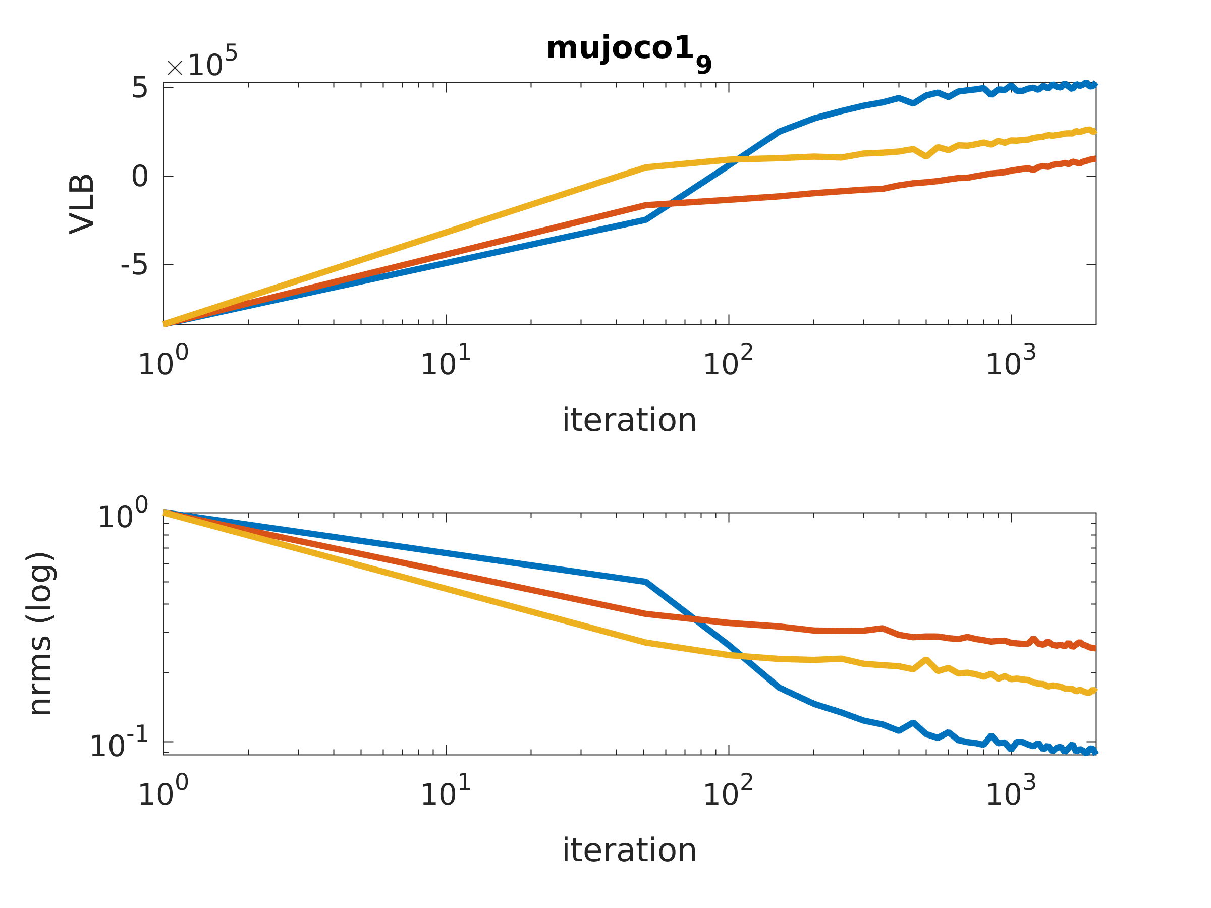
(a) Sample Complexity

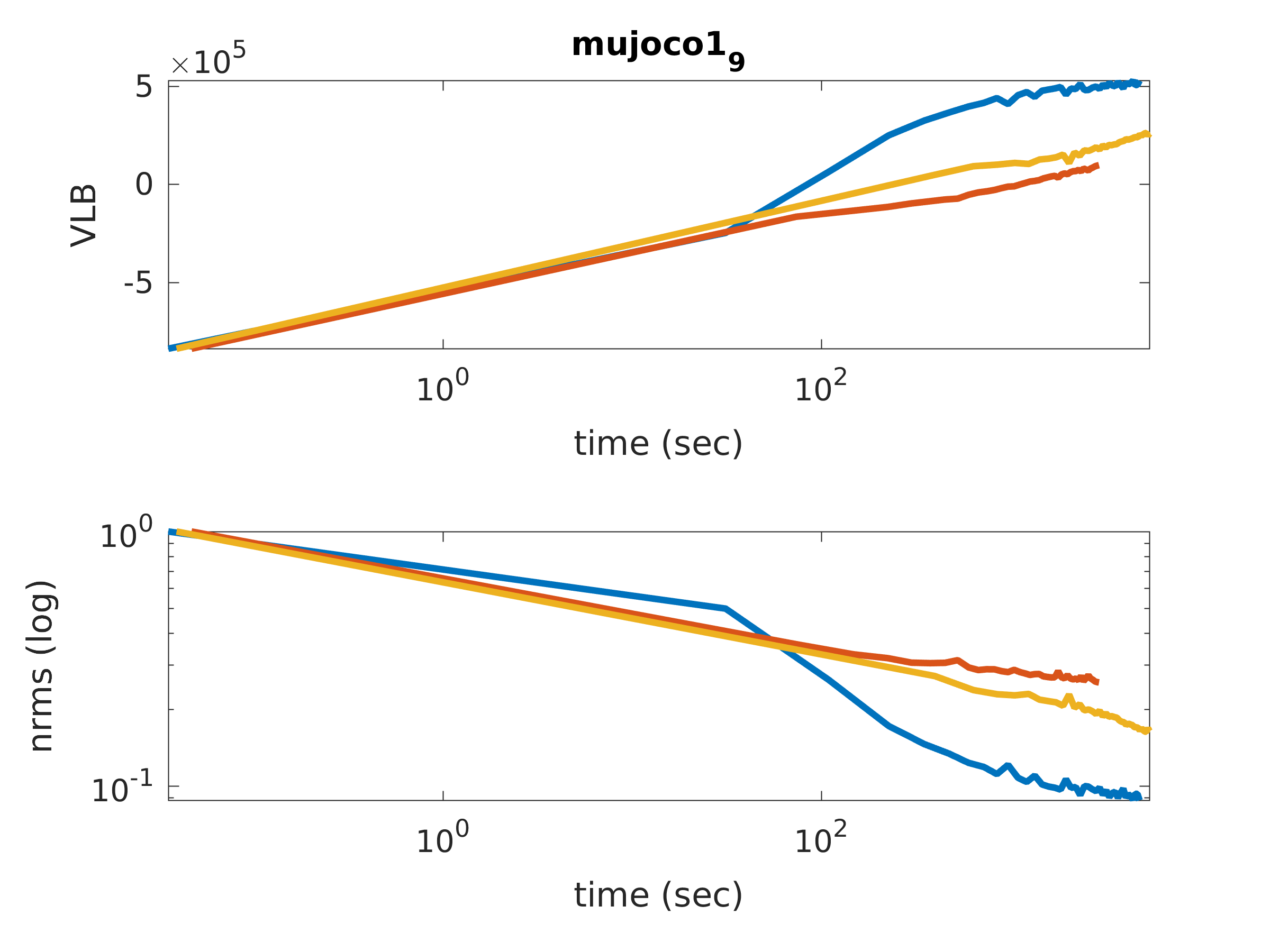
(b) Time Complexity

Figure 2: An example of online learning results (the 9th output of mujoco₁ dataset). The blue, red, and yellow lines denote svdgp, svi, and ivsgpr, respectively.

4.2 Results

We summarize part of the experimental results in Table 2 in terms of nMSE in prediction and VLB. While each output is treated independently during learning, Table 2 present the mean and the standard deviation over all the outputs as the selected metrics are normalized. For the complete experimental results, please refer to Appendix D.

We observe that svdgp consistently outperforms the other approaches with much higher VLBs and much lower prediction errors; svdgp also has smaller standard deviation. These results validate our initial hypothesis that adopting a large set of basis functions for the mean can help when modeling complicated functions. ivsgpr has the next best result after svdgp, despite using a basis size of 256, much smaller than that of 1,024 in svi, vsgpr, and gpr. Similar to svdgp, ivsgpr also generalizes better than the batch algorithms vsgpr and gpr, which only have access to a smaller set of training data and are more prone to over-fitting. By contrast, the performance of svi is surprisingly worse than vsgpr. We conjecture this might be due to the fact that the hyper-parameters and the inducing points/functions are only crudely initialized in online learning. We additionally find that the stability of svi is more sensitive to the choice of step size than other methods. This might explain why in [10, 2] batch data was used to initialize the hyper-parameters and the learning rate to update the hyper-parameters was selected to be much smaller than that for stochastic natural gradient ascent.

To further investigate the properties of different stochastic approximations, we show the change of VLB and the prediction error over iterations and time in Figure 2. Overall, whereas ivsgpr and svi share similar convergence rate, the behavior of svdgp is different. We see that ivsgpr converges the fastest, both in time and sample complexity. Afterwards, svdgp starts to descend faster and surpass the other two methods. From Figure 2, we can also observe that although svi has similar convergence to ivsgpr, it slows down earlier and therefore achieves a worse result. These phenomenon are observed in multiple experiments.

5 Conclusion

We propose a novel, fully-differentiable framework, Decoupled Gaussian Processes DGPs, for large-scale GP problems. By decoupling the representation, we derive a variational inference problem that can be solved with stochastic gradients with linear time and space complexity. Compared with existing algorithms, svdgp can adopt a much larger set of basis functions to predict more accurately. Empirically, svdgp significantly outperforms state-of-the-arts variational sparse GPR algorithms in multiple regression tasks. These encouraging experimental results motivate further application of svdgp to end-to-end learning with neural networks in large-scale, complex real world problems.

Acknowledgments

This work was supported in part by NSF NRI award 1637758. The authors additionally thank the reviewers and Hugh Salimbeni for productive discussion which improved the quality of the paper.

Appendix

Appendix A Subspace Parametrization and Notes to Practitioners

As mentioned in Section 3.3, the choice of subspace parametrization is non-unique and not limited to

$$\tilde{\mu} =\Psi_{\alpha}\mathbf{a},\quad\tilde{\Sigma}=(I+\Psi_{\beta}\mathbf{B}\Psi_{\beta}^{T})^{-1}.$$

While we adopted the completely decoupled, directly parametrized representation in the experiments for its simplicity and sufficiency to validate our idea, this choice may not possess the best numerical properties. Here we point out other potential, practical parameterizations. A complete study of these choices is outside of the scope of this paper.

A.1 Numerical Convergence Issues

To understand the effect of the parametrization on the convergence rate, intuition can be gained by inspecting the objective function $\max_{q(f),\theta}\mathbb{E}_{q}[\log p_{\theta}(y|f)]-\mathrm{KL}[q||p]$, where

$$\mathrm{KL}[q||p] =\frac{1}{2}\mathbf{a}^{T}\mathbf{K}_{{\alpha}}\mathbf{a}+\frac{1}{2}\log|\mathbf{I}+\mathbf{K}_{{\beta}}\mathbf{B}|+\frac{-1}{2}\mathrm{tr}\left(\mathbf{K}_{\beta}(\mathbf{B}^{-1}+\mathbf{K}_{{\beta}})^{-1}\right)$$

$$\mathbb{E}_{q}[\log p_{\theta}(y|f)] =\sum_{n=1}^{N}\mathbb{E}_{q({f(x_{n})})}[\log p_{\theta}(y_{n}|f(x_{n}))]$$

When the likelihood function is Gaussian, this leads to a problem which is quadratic in $\mathbf{a}$. Therefore, the numerical convergence rate can be slow, for example, when $\mathbf{K}_{\alpha}$ is ill-conditioned (which can happen especially when $M_{\alpha}$ is large and $\Psi_{\alpha}$ is not flexible and correlated). Empirically, we observed a slow-down of convergence rate when the standard se-ard kernel was used as the variational basis, compared with the generalized se-ard kernel used in the experiments.

The use of a preconditioner can help the convergence of first-order methods in practice. This can be achieved by further parameterizing $(\mathbf{a},\mathbf{B})$. For example, a Jacobi preconditioner can be optionally used in implementation by parameterizing $\mathbf{a}$ and $\mathbf{L}$ (i.e. $\mathbf{B}=\mathbf{L}\mathbf{L}^{T}$) through $\mathbf{a}_{0}$ and $\mathbf{L}_{0}$ as

$$\mathbf{a}=\mathrm{diag}(\mathbf{K}_{\alpha})^{-1}\mathbf{a}_{0},\qquad\mathbf{L}=\mathrm{diag}(\mathbf{K}_{\beta})^{-1}\mathbf{L}_{0}$$

where $\mathrm{diag}$ denotes the diagonal part. While the Jacobi preconditioner is only $\rho^{-2}\mathbf{I}$ for se-ard kernels for some scaling constant $\rho\in\mathbb{R}$, we observed it still helps the convergence rate as the hyperparameter $\rho$ is also being updated online.

Comparing the Jacobi preconditioner and (4), we can see that the canonical parametrization in (4) can be viewed as a full preconditioner, which can enjoy a better numerical convergence rate but at the cost of higher computational complexity. For the mean function, this type of full preconditioner, with $\mathbf{K}_{\alpha}^{-1}$, is too expensive to compute when $M_{\alpha}$ is large; nonetheless, using an approximation, such as the Nyström approximation or (incomplete) Cholesky decomposition, can potentially improve convergence without increasing the computational complexity. For the covariance function, because $M_{\beta}$ is small, a full preconditioner can be used, such as setting $\mathbf{L}=\mathbf{K}_{\beta}^{-1}\mathbf{L}_{0}$ or parameterizing $\mathbf{B}$ with the canonical choice (4) (see Appendix A.3 for a further discussion).

A.2 Non-convexity and Initialization

Since the optimization problem is non-convex, the performance of the model also hinges on how the variational basis functions are initialized. We note that, when using the completely decoupled parametrization as in the experiments, we advocate to initialize the new basis for the mean and the covariance to be the same samples (e.g. from the current mini-batch) and then updating them separately online. This would encourage $\tilde{\mu}$ and $\tilde{\Sigma}$ to capture the information in a close subspace.

Another idea to improve stability is to partially share the basis functions. For example, the first $M_{\beta}$ basis functions of the total $M_{\alpha}$ basis functions for the mean can be constrained to be the same as the basis functions for the covariance. Due to the redundancy in the mean parametrization, sharing part of the parameters can make the problem more well-conditioned and easier to optimize.

A.3 Hybrid Subspace Parametrization

An example that combines the ideas from the above two sections is a hybrid subspace parametrization of the variational Gaussian measure:

$$\tilde{\mu}=\Psi_{\tilde{X}}\mathbf{K}_{\tilde{X}}^{-1}\tilde{\mathbf{m}}+\Psi_{\alpha_{r}}\mathbf{a}_{r}\qquad\tilde{\Sigma}=I+\Psi_{\tilde{X}}\mathbf{K}_{\tilde{X}}^{-1}\left(\tilde{\mathbf{S}}-\mathbf{K}_{\tilde{X}}\right)\mathbf{K}_{\tilde{X}}^{-1}\Psi_{\tilde{X}}^{T}$$ (11)

where $\tilde{\mathbf{m}}\in\mathbb{R}^{M}$ and $\tilde{\mathbf{S}}\succeq 0\in\mathbb{R}^{M\times M}$ are equivalent to the posterior statistics on $\tilde{X}$ used in the conventional shared representation, $\alpha_{r}$ denotes the additional inducing points that model the residual error, and $\mathbf{a}_{r}$ is the corresponding coefficient. This representation is equivalent to setting $\beta=\tilde{X}$ and $\mathbf{B}^{-1}=-(\mathbf{K}_{\tilde{X}}+\mathbf{K}_{\tilde{X}}(\tilde{\mathbf{S}}-\mathbf{K}_{\tilde{X}})^{-1}\mathbf{K}_{\tilde{X}})$. The hybrid subspace parametrization gives a predictive model in the form

$$\hat{m}_{|\mathbf{y}}^{H}(x) =\mathbf{k}_{x,\tilde{X}}\mathbf{K}_{\tilde{X}}^{-1}\tilde{\mathbf{m}}+\mathbf{k}_{x,\alpha_{r}}\mathbf{a}_{r}$$ (12)

$$\hat{k}_{|\mathbf{y}}^{H}(x,x^{\prime}) =k_{x,x^{\prime}}+\mathbf{k}_{x,\tilde{X}}\mathbf{K}_{\tilde{X}}^{-1}\left(\tilde{\mathbf{S}}-\mathbf{K}_{\tilde{X}}\right)\mathbf{K}_{\tilde{X}}^{-1}\mathbf{k}_{\tilde{X},x^{\prime}}$$ (13)

Compared with (4), the only difference is the residual term $\mathbf{k}_{x,\alpha_{r}}\mathbf{a}_{r}$, which helps modeling more complex functions.

Therefore, this new, hybrid formulation shows a more direct connection to the conventional parametrization used in the GP literature (e.g. [11]). This can also been seen in its associated objective function. Substitute the hybrid parametrization into the terms in the KL divergence between Gaussian measures and we have the following relations:

$$\frac{1}{2}\mathbf{a}^{T}\mathbf{K}_{{\alpha}}\mathbf{a}=\frac{1}{2}\tilde{\mathbf{m}}^{T}\mathbf{K}_{\tilde{X}}^{-1}\tilde{\mathbf{m}}+\tilde{\mathbf{m}}^{T}\mathbf{K}_{\tilde{X}}^{-1}\mathbf{K}_{\tilde{X},\alpha_{r}}\mathbf{a}_{r}+\frac{1}{2}\mathbf{a}_{r}^{T}\mathbf{K}_{\alpha_{r}}\mathbf{a}_{r}$$

$$\frac{-1}{2}\mathrm{tr}\left(\mathbf{K}_{\beta}(\mathbf{B}^{-1}+\mathbf{K}_{{\beta}})^{-1}\right)=\frac{1}{2}\mathrm{tr}\left(\tilde{\mathbf{S}}\mathbf{K}_{\tilde{X}}^{-1}\right)-\frac{|\tilde{X}|}{2}$$

$$\frac{1}{2}\log|\mathbf{I}+\mathbf{K}_{{\beta}}\mathbf{B}|=-\log|\mathbf{K}_{\tilde{X}}^{-1}\tilde{\mathbf{S}}|.$$

Therefore, the KL divergence term for the hybrid parametrization can be written as

$$\mathrm{KL}[q||p] =\frac{1}{2}\tilde{\mathbf{m}}^{T}\mathbf{K}_{\tilde{X}}^{-1}\tilde{\mathbf{m}}+\tilde{\mathbf{m}}^{T}\mathbf{K}_{\tilde{X}}^{-1}\mathbf{K}_{\tilde{X},\alpha_{r}}\mathbf{a}_{r}+\frac{1}{2}\mathbf{a}_{r}^{T}\mathbf{K}_{\alpha_{r}}\mathbf{a}_{r}$$

$$\quad-\log|\mathbf{K}_{\tilde{X}}^{-1}\tilde{\mathbf{S}}|+\frac{1}{2}\mathrm{tr}\left(\tilde{\mathbf{S}}\mathbf{K}_{\tilde{X}}^{-1}\right)-\frac{|\tilde{X}|}{2}$$ (14)

This KL divergence terms is exactly as the one used by Hensman et al. [11], when $\tilde{\mathbf{a}}_{r}=0$. That is, the hybrid parametrization is a strict generalization of the canonical parametrization. Note in here $\tilde{\mathbf{S}}$ is initialized as $\tilde{\mathbf{S}}=\tilde{\mathbf{K}}_{\tilde{X}}=\mathbf{L}\mathbf{L}^{T}$ and then its Cholesky factor $\mathbf{L}$ is optimized afterwards.

From (12), (13), and (14), we can see the linear complexity of the decoupled model is preserved. The stochastic gradient can be computed in linear time by performing sampling of the residual inducing points $\alpha_{r}$.

Appendix B Variational Inference with Decoupled Gaussian Processes

Here we provide the details of the variational inference problem used to learn DGPs:

$$\max_{q(f),\theta}\mathcal{L}_{\theta}(q(f) =\max_{q(f),\theta}\int q(f)\log\frac{p_{\theta}(y|f)p(f)}{q(f)}\mathrm{d}{f}=\max_{q(f),\theta}\mathbb{E}_{q}[\log p_{\theta}(y|f)]-\mathrm{KL}[q||p],$$ (15)

B.1 KL Divergence

B.1.1 Evaluation

First, we show how to evaluate the KL-divergence. We do so by extending the KL-divergence between two finite-dimensional subspace-parametrized Gaussian measures to infinite dimensional space and show that it is well-defined.

Recall for two $d$-dimensional Gaussian distributions $q(f)=\mathcal{N}(f|\mu,\Sigma)$ and $p=\mathcal{N}(f|\bar{\mu},\bar{\Sigma})$, the KL-divergence is given as

Proposition 1.

$$\mathrm{KL}[q||p] :=\int\log\frac{q(f)}{p(f)}\mathrm{d}\mu_{q}(f)=\int q(f)\log\frac{q(f)}{p(f)}\mathrm{d}f$$

$$=\frac{1}{2}\left(\mathrm{tr}\left(\bar{\Sigma}^{-1}{\Sigma}\right)+({\mu}-\bar{\mu})^{T}\bar{\Sigma}^{-1}({\mu}-\bar{\mu})+\ln\frac{|\bar{\Sigma}|}{|\Sigma|}-d\right)$$

Now consider $q$ and $p$ are subspace parametrized as

$$\begin{matrix}p(f)=\mathcal{N}(f|\bar{\mu},\bar{\Sigma})=\mathcal{N}(f|\Psi_{\bar{\alpha}}\bar{\mathbf{a}},(I+\Psi_{\bar{\beta}}\bar{\mathbf{B}}\Psi_{\bar{\beta}}^{T})^{-1})\\ q(f)=\mathcal{N}({f|\mu},{\Sigma})=\mathcal{N}(f|\Psi_{\alpha}{\mathbf{a}},(I+\Psi_{\beta}{\mathbf{B}}\Psi_{\beta}^{T})^{-1}).\end{matrix}$$ (16)

By Proposition 1, we derive the representation of KL-divergence which is applicable even when $d$ is infinite. Recall in the infinite dimensional case, $\mu$, $\Sigma$, $\bar{\mu}$, and $\bar{\Sigma}$ are objects in the RKHS $\mathcal{H}$ (Cameron-Martin space).

Theorem 1.

Assume $q$ and $p$ are two subspace parametrized Gaussian measures given as (16). Regardless of the dimension of $\mathcal{H}$, the following holds

$$\mathrm{KL}[q||p] =\frac{-1}{2}\mathrm{tr}\left(\left(\mathbf{K}_{\beta}+\mathbf{K}_{{\beta},\bar{\beta}}\bar{\mathbf{B}}\mathbf{K}_{\bar{\beta},{\beta}}\right)({\mathbf{B}}^{-1}+\mathbf{K}_{{\beta}})^{-1}\right)+\frac{1}{2}\log|\mathbf{I}+\mathbf{K}_{{\beta}}{\mathbf{B}}|$$

$$\quad+\frac{1}{2}{\mathbf{a}}^{T}\left(\mathbf{K}_{{\alpha}}+\mathbf{K}_{{\alpha},\bar{\beta}}\bar{\mathbf{B}}\mathbf{K}_{\bar{\beta},{\alpha}}\right){\mathbf{a}}-{\mathbf{a}}^{T}\left(\mathbf{K}_{{\alpha},\bar{\alpha}}+\mathbf{K}_{{\alpha},\bar{\beta}}\bar{\mathbf{B}}\mathbf{K}_{\bar{\beta},\bar{\alpha}}\right)\bar{\mathbf{a}}+C$$ (17)

where

$$C=\frac{1}{2}\left(\mathrm{tr}\left(\mathbf{K}_{\bar{\beta}}\bar{\mathbf{B}}\right)-\log|\mathbf{I}+\mathbf{K}_{\bar{\beta}}\bar{\mathbf{B}}|+\bar{\mathbf{a}}^{T}\left(\mathbf{K}_{{\bar{\alpha}}}+\mathbf{K}_{{\bar{\alpha}},\bar{\beta}}\mathbf{\bar{B}}\mathbf{K}_{\bar{\beta},{\bar{\alpha}}}\right)\bar{\mathbf{a}}\right)$$

In particular, if $p$ is normal (i.e. $p(f)=\mathcal{N}(f|0,I)$), then

$$\mathrm{KL}[q||p] =\frac{1}{2}\mathbf{a}^{T}\mathbf{K}_{{\alpha}}\mathbf{a}+\frac{1}{2}\log|\mathbf{I}+\mathbf{K}_{{\beta}}\mathbf{B}|+\frac{-1}{2}\mathrm{tr}\left(\mathbf{K}_{\beta}(\mathbf{B}^{-1}+\mathbf{K}_{{\beta}})^{-1}\right)$$

Proof.

To prove, we derive each term in (17) as follows.

First, we derive $\mathrm{tr}\left(\bar{\Sigma}^{-1}{\Sigma}\right)-d$. Define $\mathbf{R}=(\mathbf{B}^{-1}+\mathbf{K}_{\beta})^{-1}$. Then we can write

$$\Sigma =(I+\Psi_{\beta}\mathbf{B}\Psi_{\beta}^{T})^{-1}=I-\Psi_{\beta}(\mathbf{B}^{-1}+\Psi_{\beta}^{T}\Psi_{\beta})^{-1}\Psi_{\beta}^{T}=I-\Psi_{\beta}\mathbf{R}\Psi_{\beta}^{T}.$$ (18)

Using (18), we can derive

$$\bar{\Sigma}^{-1}{\Sigma} =(I+\Psi_{\bar{\beta}}\bar{\mathbf{B}}\Psi_{\bar{\beta}}^{T})\left(I-\Psi_{\beta}\mathbf{R}\Psi_{\beta}^{T}\right)=I+\Psi_{\bar{\beta}}\bar{\mathbf{B}}\Psi_{\bar{\beta}}^{T}-\Psi_{\beta}\mathbf{R}\Psi_{\beta}^{T}-\Psi_{\bar{\beta}}\mathbf{\bar{B}}\mathbf{K}_{\bar{\beta},{\beta}}\mathbf{R}\Psi_{\beta}^{T}$$

and therefore

$$\mathrm{tr}\left(\bar{\Sigma}^{-1}{\Sigma}\right)-d =\mathrm{tr}\left(I\right)-d+\mathrm{tr}\left(\mathbf{K}_{\bar{\beta}}\bar{\mathbf{B}}\right)-\mathrm{tr}\left(\mathbf{R}\left(\mathbf{K}_{\beta}+\mathbf{K}_{{\beta},\bar{\beta}}\bar{\mathbf{B}}\mathbf{K}_{\bar{\beta},{\beta}}\right)\right)$$

$$=\mathrm{tr}\left(\mathbf{K}_{\bar{\beta}}\bar{\mathbf{B}}\right)-\mathrm{tr}\left(\mathbf{R}\left(\mathbf{K}_{\beta}+\mathbf{K}_{{\beta},\bar{\beta}}\bar{\mathbf{B}}\mathbf{K}_{\bar{\beta},{\beta}}\right)\right)$$

Note this term does not depend on the ambient dimension.

Second, we derive $\log(|\bar{\Sigma}|/|{\Sigma}|)$: Since

$$\log|{\Sigma}^{-1}|=\log|\mathbf{B}^{-1}+\mathbf{K}_{\beta}||\mathbf{B}|=\log|\mathbf{I}+\mathbf{K}_{\beta}\mathbf{B}|.$$

it holds that

$$\log\frac{|\bar{\Sigma}|}{|{\Sigma}|}=\log|\mathbf{I}+\mathbf{K}_{\beta}\mathbf{B}|-\log|\mathbf{I}+\mathbf{K}_{\bar{\beta}}\bar{\mathbf{B}}|.$$

Finally, we derive the quadratic term:

$$({\mu}-\bar{\mu})^{T}\bar{\Sigma}^{-1}({\mu}-\bar{\mu})$$

$$={\mu}^{T}\bar{\Sigma}^{-1}{\mu}-2\bar{\mu}^{T}\bar{\Sigma}^{-1}\mu+\bar{\mu}\bar{\Sigma}^{-1}\bar{\mu}$$

$$={\mathbf{a}}^{T}\Psi_{\alpha}^{T}\left(I+\Psi_{\bar{\beta}}\mathbf{\bar{B}}\Psi_{\bar{\beta}}^{T}\right)\Psi_{\alpha}{\mathbf{a}}-2{\mathbf{\bar{a}}}^{T}\Psi_{\bar{\alpha}}^{T}\left(I+\Psi_{\bar{\beta}}\bar{\mathbf{B}}\Psi_{\bar{\beta}}^{T}\right)\Psi_{\alpha}{\mathbf{a}}+{\bar{\mathbf{a}}}^{T}\Psi_{\bar{\alpha}}^{T}\left(I+\Psi_{\bar{\beta}}\mathbf{\bar{B}}\Psi_{\bar{\beta}}^{T}\right)\Psi_{\bar{\alpha}}\bar{5}{\mathbf{a}}$$

$$={\mathbf{a}}^{T}\left(\mathbf{K}_{{\alpha}}+\mathbf{K}_{{\alpha},\bar{\beta}}\mathbf{\bar{B}}\mathbf{K}_{\bar{\beta},{\alpha}}\right){\mathbf{a}}-2{\mathbf{\bar{a}}}^{T}\left(\mathbf{K}_{\bar{\alpha},{\alpha}}+\mathbf{K}_{\bar{\alpha},\bar{\beta}}\mathbf{\bar{B}}\mathbf{K}_{\bar{\beta},{\alpha}}\right){\mathbf{a}}+\bar{\mathbf{a}}^{T}\left(\mathbf{K}_{{\bar{\alpha}}}+\mathbf{K}_{{\bar{\alpha}},\bar{\beta}}\mathbf{\bar{B}}\mathbf{K}_{\bar{\beta},{\bar{\alpha}}}\right)\bar{\mathbf{a}}$$

∎

Remarks

The above expression is well defined even when $\mathbf{B}\succeq 0$, because $({\mathbf{B}}^{-1}+\mathbf{K}_{{\beta}})^{-1}=\mathbf{B}(\mathbf{I}+\mathbf{K}_{{\beta}}\mathbf{B})^{-1}$. Particularly, we can parametrize $\mathbf{B}=\mathbf{L}\mathbf{L}^{T}$ with Cholesky factor $\mathbf{L}\in\mathbb{R}^{M_{\beta}\times M_{\beta}}$ in practice so the problem is unconstrained. The required terms can be stably computed: $\left(\mathbf{B}^{-1}+\mathbf{K}_{\beta}\right)^{-1}=\mathbf{L}\mathbf{H}^{-1}\mathbf{L}^{T}$ and $\log|\mathbf{I}+\mathbf{K}_{{\beta}}\mathbf{B}|=\log|\mathbf{H}|$, where $\mathbf{H}=\mathbf{I}+\mathbf{L}^{T}\mathbf{K}_{\beta}\mathbf{L}$.

B.1.2 Gradients

Here we derive the equations of the gradient of the variational inference problem of svdgp. The purpose here is to show the complexity of calculating the gradients. These equations are useful in implementing svdgp using basic linear algebra routines, while computational-graph libraries based on automatic differentiation are also applicable and easier to apply.

To derive the gradients, we first introduce some short-hand

$$\mathbf{G}_{\alpha} =\mathbf{K}_{{\alpha}}+\mathbf{K}_{{\alpha},\bar{\beta}}\bar{\mathbf{B}}\mathbf{K}_{\bar{\beta},{\alpha}}$$

$$\mathbf{G}_{\alpha,\bar{\alpha}} =\mathbf{K}_{{\alpha},\bar{\alpha}}+\mathbf{K}_{{\alpha},\bar{\beta}}\bar{\mathbf{B}}\mathbf{K}_{\bar{\beta},\bar{\alpha}}$$

$$\mathbf{G}_{\beta} =\mathbf{K}_{\beta}+\mathbf{K}_{{\beta},\bar{\beta}}\bar{\mathbf{B}}\mathbf{K}_{\bar{\beta},{\beta}}$$

and write $\mathrm{KL}[q||p]$ as

$$\mathrm{KL}[q||p]=\frac{-1}{2}\mathrm{tr}\left(\mathbf{G}_{\beta}({\mathbf{B}}^{-1}+\mathbf{K}_{{\beta}})^{-1}\right)+\frac{1}{2}\log|\mathbf{I}+\mathbf{K}_{{\beta}}{\mathbf{B}}|+\frac{1}{2}{\mathbf{a}}^{T}\mathbf{G}_{\alpha}{\mathbf{a}}-{\mathbf{a}}^{T}\mathbf{G}_{\alpha,\bar{\alpha}}\bar{\mathbf{a}}.$$

We then give the equations to compute the derivatives below. For compactness of notation, we use $\odot$ to denote element-wise product and use $\mathbf{1}$ to denote the vector of ones. In addition, we introduce a linear operator $\mathrm{diag}$ with overloaded definitions:

1. $\mathrm{diag}:\mathbb{R}^{N}\to\mathbb{R}^{N\times N}$ which constructs a diagonal matrix from a vector

2. $\mathrm{diag}:\mathbb{R}^{N\times N}\to\mathbb{R}^{N}$ which extracts the diagonal elements of a matrix to a vector.

Proposition 2.

The gradients of $\mathrm{KL}[q||p]$ is as follows:

$$\nabla_{\mathbf{a}}\mathrm{KL}[q||p] =\mathbf{G}_{\alpha}\mathbf{a}-\mathbf{G}_{\alpha,\bar{\alpha}}\bar{\mathbf{a}}$$

$$\nabla_{\alpha}\mathrm{KL}[q||p] =\mathrm{diag}(\mathbf{a})\left(\partial_{\alpha}\mathbf{G}_{\alpha}\mathbf{a}-\partial_{\alpha}\mathbf{G}_{\alpha,\bar{\alpha}}\bar{\mathbf{a}}\right)$$

$$\nabla_{\mathbf{B}}\mathrm{KL}[q||p] =\frac{1}{2}(\mathbf{I}+\mathbf{K}_{{\beta}}\mathbf{B})^{-1}\left(\mathbf{K}_{{\beta}}\mathbf{B}\mathbf{K}_{{\beta}}-\mathbf{\Delta}_{\beta}\right)(\mathbf{I}+\mathbf{B}\mathbf{K}_{{\beta}})^{-1}$$

$$\nabla_{\beta}\mathrm{KL}[q||p] =\left(\partial_{\beta}\mathbf{K}_{\beta}\odot({\mathbf{B}}^{-1}+\mathbf{K}_{{\beta}})^{-1}\mathbf{G}_{\beta}({\mathbf{B}}^{-1}+\mathbf{K}_{{\beta}})^{-1}\right)\mathbf{1}-\left(\partial_{\beta}\mathbf{\Delta}_{\beta}\odot(\mathbf{B}^{-1}+\mathbf{K}_{{\beta}})^{-1}\right)\mathbf{1}$$

where $\mathbf{\Delta}_{\beta}=\mathbf{G}_{\beta}-\mathbf{K}_{\beta}$ and $\partial$ is defined as the partial derivative with respect to the left argument. In particular, if the $p$ is normal,

$$\nabla_{\mathbf{a}}\mathrm{KL}[q||p] =\mathbf{K}_{\alpha}\mathbf{a}$$

$$\nabla_{\alpha}\mathrm{KL}[q||p] =\mathrm{diag}(\mathbf{a})\partial_{\alpha}\mathbf{K}_{\alpha}\mathbf{a}$$

$$\nabla_{\mathbf{B}}\mathrm{KL}[q||p] =\frac{1}{2}(\mathbf{I}+\mathbf{K}_{{\beta}}\mathbf{B})^{-1}\mathbf{K}_{{\beta}}\mathbf{B}\mathbf{K}_{{\beta}}(\mathbf{I}+\mathbf{B}\mathbf{K}_{{\beta}})^{-1}$$

$$\nabla_{\beta}\mathrm{KL}[q||p] =\left(\partial_{\beta}\mathbf{K}_{\beta}\odot({\mathbf{B}}^{-1}+\mathbf{K}_{{\beta}})^{-1}\mathbf{K}_{\beta}({\mathbf{B}}^{-1}+\mathbf{K}_{{\beta}})^{-1}\right)\mathbf{1}$$

The derivation of Proposition 2 is simply mechanical, so we omit it here.

Here we only show the derivative with respect to $\mathbf{B}$. Suppose $\mathbf{B}=\mathbf{L}\mathbf{L}^{T}$. Then one can apply the chain rule and get

$$\nabla_{\mathbf{L}}\mathrm{KL}[q||p]=2\nabla_{B}\mathrm{KL}[q||p]\mathbf{L}.$$

B.2 Expected Log-Likelihood

B.2.1 Evaluation

The evaluation of the expected log-likelihood depends on the mean and covariance in (8) , which we repeat here

$$\hat{m}_{|\mathbf{y}}^{\alpha}(x)=\mathbf{k}_{x,\alpha}\bm{a},\qquad\hat{k}_{|\mathbf{y}}^{\beta}(x,x^{\prime})=k_{x,x^{\prime}}-\mathbf{k}_{x,\beta}\left(\mathbf{B}^{-1}+\mathbf{K}_{\beta}\right)^{-1}\mathbf{k}_{\beta,x^{\prime}}.$$

Its derivation is trivial by the definition of $q$ in (16) and (18). For $N$ observations, the vector form $\hat{\mathbf{m}}\in\mathbb{R}^{N}$ and $\hat{\mathbf{s}}\in\mathbb{R}^{N}$ of the mean and the covariance above evaluated on each observation can be computed in $O(N)$ as

$$\hat{\mathbf{m}} =\mathbf{K}_{X,\alpha}\mathbf{a}$$

$$\hat{\mathbf{s}} =\mathrm{diag}\left(\mathbf{K}_{X}-\mathbf{K}_{X,\beta}(\mathbf{B}^{-1}+\mathbf{K}_{\beta})^{-1}\mathbf{K}_{\beta,X}\right)$$

$$=\mathrm{diag}(\mathbf{K}_{X})-\left(\mathbf{K}_{X,\beta}\odot(\mathbf{K}_{X,\beta}(\mathbf{B}^{-1}+\mathbf{K}_{\beta})^{-1})\right)\mathbf{1}$$

$$=\mathrm{diag}(\mathbf{K}_{X})-\left(\mathbf{K}_{X,\beta}\odot(\mathbf{K}_{X,\beta}\mathbf{B}(\mathbf{I}+\mathbf{K}_{\beta}\mathbf{B})^{-1})\right)\mathbf{1}.$$

Given $\hat{\mathbf{m}}$ and $\hat{\mathbf{s}}$, the expected log-likelihood can be evaluated either in closed-form for Gaussian likelihood or by sampling for general likelihoods.

B.2.2 Gradients

The computation of the gradients of the expected log-likelihood can be completed in two steps. First, we compute the gradients of $\mathbb{E}_{q}[\log p_{\theta}(y|f)]$ with respect to $(\theta,\hat{\mathbf{m}},\hat{\mathbf{s}})$ (i.e. $\nabla_{\hat{\mathbf{m}}}e$, $\nabla_{\hat{\mathbf{s}}}e$, and $\nabla_{\hat{\mathbf{\theta}}}e$ ). Because $\log p_{\theta}(y|f)$ is the sum of $N$ terms, this step can be done in $O(N)$: for each observation $x$, let $q(f(x))=\mathcal{N}(f(x)|\hat{m},\hat{s})$ be a scalar Gaussian; under standard regularity conditions, we have

$$\nabla_{\hat{m}}\mathbb{E}_{q}[\log p_{\theta}(y|f(x))] =\mathbb{E}_{q}[\nabla_{\hat{m}}\log q(f(x))\log p_{\theta}(y|f(x))]$$

$$\nabla_{\hat{s}}\mathbb{E}_{q}[\log p_{\theta}(y|f(x))] =\mathbb{E}_{q}[\nabla_{\hat{s}}\log q(f(x))\log p_{\theta}(y|f(x))]$$

$$\nabla_{\theta}\mathbb{E}_{q}[\log p_{\theta}(y|f(x))] =\mathbb{E}_{q}[\nabla_{\theta}\log p_{\theta}(y|f(x))]$$

where $\nabla_{\theta}\log p_{\theta}(y|f(x))$ can be found, for example, in [22]. The above can be calculated in closed-form for Gaussian likelihood or by sampling for general likelihoods.

Next we propagate these gradients by chain rule. The results are summarized below.

Proposition 3.

Let $e=\mathbb{E}_{q}[\log p_{\theta}(y|f)]$. Suppose $k(x,x^{\prime})=\rho^{2}g_{s}(x,x^{\prime})$ for some hyper-parameters $\rho,s\in\mathbb{R}$. The gradients of e are as follows:

$$\nabla_{a}e =\mathbf{K}_{X,\alpha}^{T}\nabla_{\hat{\mathbf{m}}}e$$

$$\nabla_{\alpha}e =\mathrm{diag}(\mathbf{a})\partial\mathbf{K}_{X,\alpha}^{T}\nabla_{\hat{\mathbf{m}}}e$$

$$\nabla_{\mathbf{B}}e =-(\mathbf{I}+\mathbf{K}_{\beta}\mathbf{B})^{-1}\mathbf{K}_{X,\beta}^{T}\mathrm{diag}(\nabla_{\hat{\mathbf{s}}}e)\mathbf{K}_{X,\beta}(\mathbf{I}+\mathbf{B}\mathbf{K}_{\beta})^{-1}$$

$$\nabla_{\beta}\hat{e} =2(\partial\mathbf{K}_{\beta}^{T}\odot(\mathbf{\Omega}\mathrm{diag}(\nabla_{\hat{\mathbf{s}}}e)\mathbf{\Omega}^{T}))\bm{1}-2(\mathbf{\Omega}\odot\partial\mathbf{K}_{\beta,X})\nabla_{\hat{\mathbf{s}}}e$$

$$\nabla_{\log\rho}e =\hat{\mathbf{m}}^{T}\nabla_{\hat{\mathbf{m}}}e+2\hat{\mathbf{s}}^{T}\nabla_{\hat{{\mathbf{s}}}}e$$

$$\nabla_{s}e =(\partial_{s}\mathbf{K}_{X,\alpha}\mathbf{a})^{T}\nabla_{\hat{\mathbf{m}}}e-2\bm{1}^{T}\left(\mathbf{\Omega}\odot\partial_{s}\mathbf{K}_{\beta,X}\right)\nabla_{\hat{{\mathbf{s}}}}e$$

where $\mathbf{\Omega}=\mathbf{B}(\mathbf{I}+\mathbf{K}_{\beta}\mathbf{B})^{-1}\mathbf{K}_{\beta,X}$.

The derivation of Proposition 3 is only technical, so we omit it here.

Appendix C Experiment Setup

C.1 The Covariance Function

For all the models, we assume the prior is zero mean and has covariance defined by a se-ard kernel [19]

$$k(x,x^{\prime})=\rho^{2}\phi_{x}^{T}\phi_{x}=\rho^{2}\prod_{d=1}^{D}\exp(\frac{-(x_{d}-x^{\prime}_{d})^{2}}{2s_{d}^{2}}),$$

where $s_{d}>0$ is the length scale of dimension $d$. For the variational posterior, we use the generalized se-ard kernel [2]

$$\psi_{x}^{T}\psi_{x^{\prime}} =\prod_{d=1}^{D}\left(\frac{2l_{x,d}l_{x^{\prime},d}}{l_{x,d}^{2}+l_{x^{\prime},d}^{2}}\right)^{1/2}\exp\left(-\frac{\|x_{d}-x_{d}^{\prime}\|^{2}}{l_{x,d}^{2}+l_{x^{\prime},d}^{2}}\right),$$ (19)

where $l_{x,d}=s_{d}\cdot c_{x,d}$ is the length-scale parameter. That is, we evaluate

$$\mathbb{C}[L_{m}f(\tilde{x}_{m}),L_{n}f(\tilde{x}_{n})]=\psi_{\tilde{x}_{m}}^{T}\psi_{\tilde{x}_{n}}$$

where the associated length-scalar parameters implicitly define the linear operators $L_{m}$ and $L_{n}$.

This kernel is first introduced in [26] by convoluting a se-ard kernel with Gaussian integral kernels, and later modified into its current form (19) in [2]. From (19), we see it contains se-ard as a special case. That is, $\psi_{x}=\phi_{x}$ when $c_{x,d}=1$, $\forall d\in\{1,\dots,D\}$. But in general $c_{x,d}$ can be a function of $x$. Therefore, it can be shown that $\psi_{x}$ spans an RKHS that contains the RKHSs spanned by $\phi_{x}$ for all length-scales, and every cross covariance can be computed as $\mathbb{C}[L_{m}f(\tilde{x}_{m}),f(x)]=\rho\psi_{\tilde{x}_{m}}^{T}\phi_{x}$.

Note: all the algorithms in our comparisons use this generalized se-ard kernel.

C.2 Online Learning Procedure

Algorithm 1 summarizes the online learning procedure used by all stochastic algorithms (the algorithms differs only in whether the bases are shared and how the model is updated; see Table 1.), where each learner has to optimize all the parameters on-the-fly using i.i.d. data. The hyper-parameters are first initialized heuristically by median trick using the first mini-batch (in the GPR experiments, $s_{d}$ is initialized as the median of pairwise distances of the sampled observations; $\sigma^{2}$ is initialized as the variance of the sampled outputs; $\rho=1$). We incrementally build up the variational posterior by including $N_{\Delta}\leq N_{m}$ observations in each mini-batch as the initialization of new variational basis functions (we initialize a new variational basis as $\tilde{x}_{m}=x_{n}$ and $c_{\tilde{x},d}=1$, where $x_{n}$ is a sample from the current mini-batch). Then all the hyper-parameters and the variational parameters are updated online. These steps are repeated for $T$ iterations.

Appendix D Complete Experimental Results

D.1 Experimental Results on KUKA datasets

	svdgp	svi	ivsgpr	vsgpr	gpr
$Y_{1}$	0.985	0.336	0.411	0.085	-3.840
$Y_{2}$	1.359	0.458	0.799	0.468	-23.218
$Y_{3}$	0.951	0.312	0.543	0.158	-8.145
$Y_{4}$	1.453	0.528	0.906	0.722	-0.965
$Y_{5}$	1.350	0.311	0.377	0.425	-0.990
$Y_{6}$	1.278	0.367	0.631	0.559	-0.639
$Y_{7}$	1.458	0.425	0.877	0.886	0.449
mean	1.262	0.391	0.649	0.472	-5.335
std	0.195	0.076	0.201	0.265	7.777

(a) Variational Lower Bound ($10^{5}$)

	svdgp	svi	ivsgpr	vsgpr	gpr
$Y_{1}$	0.058	0.186	0.165	0.171	0.257
$Y_{2}$	0.028	0.146	0.095	0.126	0.249
$Y_{3}$	0.058	0.195	0.133	0.181	0.298
$Y_{4}$	0.027	0.124	0.088	0.114	0.198
$Y_{5}$	0.028	0.195	0.178	0.132	0.243
$Y_{6}$	0.034	0.178	0.137	0.140	0.224
$Y_{7}$	0.028	0.155	0.099	0.108	0.146
mean	0.037	0.169	0.128	0.139	0.231
std	0.013	0.025	0.033	0.026	0.045

(b) Prediction Error (nMSE)

Table 3: Experimental results of kuka₁ after 2,000 iteration. $Y_{i}$ denotes the $i$th output.

	svdgp	svi	ivsgpr	vsgpr	gpr
$Y_{1}$	1.047	0.398	0.631	0.399	-3.709
$Y_{2}$	1.387	0.450	0.767	0.515	-31.315
$Y_{3}$	0.976	0.321	0.568	0.232	-12.230
$Y_{4}$	1.404	0.507	0.630	0.654	-1.026
$Y_{5}$	1.332	0.317	0.378	0.511	-0.340
$Y_{6}$	1.260	0.368	0.585	0.538	-0.221
$Y_{7}$	1.405	0.437	0.519	0.918	0.526
mean	1.259	0.400	0.583	0.538	-6.902
std	0.165	0.065	0.110	0.197	10.770

(a) Variational Lower Bound ($10^{5}$)

	svdgp	svi	ivsgpr	vsgpr	gpr
$Y_{1}$	0.056	0.168	0.126	0.151	0.281
$Y_{2}$	0.026	0.147	0.102	0.124	0.248
$Y_{3}$	0.056	0.194	0.127	0.179	0.325
$Y_{4}$	0.029	0.127	0.127	0.110	0.186
$Y_{5}$	0.029	0.189	0.170	0.125	0.232
$Y_{6}$	0.035	0.181	0.144	0.144	0.232
$Y_{7}$	0.034	0.152	0.166	0.104	0.133
mean	0.038	0.166	0.137	0.134	0.234
std	0.012	0.023	0.022	0.024	0.058

(b) Prediction Error (nMSE)

Table 4: Experimental results of kuka₂ after 2,000 iterations. $Y_{i}$ denotes the $i$th output.

D.2 Experimental Results on MuJoCo datasets

	svdgp	svi	ivsgpr	vsgpr	gpr
$Y_{1}$	7.373	3.195	5.948	4.312	-22.256
$Y_{2}$	6.019	2.141	3.905	2.328	-45.351
$Y_{3}$	6.350	2.543	4.695	2.991	-147.881
$Y_{4}$	5.852	2.417	4.792	2.468	-23.999
$Y_{5}$	6.280	2.609	5.316	3.622	-8.626
$Y_{6}$	5.152	1.043	4.418	3.452	-11296.669
$Y_{7}$	5.270	2.093	4.183	1.676	-7745.055
$Y_{8}$	6.471	2.585	5.040	3.068	-47.540
$Y_{9}$	5.293	0.979	2.592	1.482	-73477.168
mean	6.007	2.178	4.543	2.822	-10312.727
std	0.673	0.692	0.898	0.871	22679.778

(a) Variational Lower Bound ($10^{5}$)

	svdgp	svi	ivsgpr	vsgpr	gpr
$Y_{1}$	0.049	0.087	0.067	0.088	0.133
$Y_{2}$	0.068	0.163	0.112	0.122	0.196
$Y_{3}$	0.064	0.134	0.091	0.112	0.213
$Y_{4}$	0.073	0.144	0.087	0.121	0.179
$Y_{5}$	0.068	0.132	0.080	0.103	0.159
$Y_{6}$	0.094	0.251	0.107	0.131	0.253
$Y_{7}$	0.084	0.168	0.100	0.145	0.348
$Y_{8}$	0.063	0.132	0.087	0.104	0.178
$Y_{9}$	0.088	0.255	0.165	0.131	0.258
mean	0.072	0.163	0.099	0.118	0.213
std	0.013	0.053	0.026	0.016	0.061

(b) Prediction Error (nMSE)

Table 5: Experimental results of mujoco₁ after 2,000 iterations. $Y_{i}$ denotes the $i$th output.

	svdgp	svi	ivsgpr	vsgpr	gpr
$Y_{1}$	7.249	3.013	6.429	4.161	-33.219
$Y_{2}$	5.994	2.475	4.800	2.770	-23.276
$Y_{3}$	6.239	2.258	4.819	3.044	-59.757
$Y_{4}$	5.935	2.093	4.489	2.547	-27.259
$Y_{5}$	6.387	2.452	5.457	3.725	-1.786
$Y_{6}$	7.320	1.087	4.639	4.043	-24.198
$Y_{7}$	5.346	1.754	3.947	1.667	-255179.052
$Y_{8}$	6.448	2.505	5.193	3.812	-190.294
$Y_{9}$	6.237	0.683	2.596	2.241	-37673.328
mean	6.350	2.036	4.708	3.112	-32579.130
std	0.586	0.699	0.993	0.825	79570.425

(a) Variational Lower Bound ($10^{5}$)

	svdgp	svi	ivsgpr	vsgpr	gpr
$Y_{1}$	0.051	0.095	0.056	0.085	0.138
$Y_{2}$	0.069	0.133	0.085	0.111	0.186
$Y_{3}$	0.066	0.149	0.087	0.113	0.182
$Y_{4}$	0.071	0.160	0.094	0.127	0.197
$Y_{5}$	0.065	0.137	0.074	0.101	0.148
$Y_{6}$	0.051	0.241	0.097	0.073	0.139
$Y_{7}$	0.081	0.187	0.107	0.142	0.363
$Y_{8}$	0.063	0.133	0.081	0.106	0.214
$Y_{9}$	0.067	0.270	0.157	0.106	0.300
mean	0.065	0.167	0.093	0.107	0.207
std	0.009	0.053	0.026	0.019	0.072

(b) Prediction Error (nMSE)

Table 6: Experimental results of mujoco₂ after 2,000 iterations. $Y_{i}$ denotes the $i$th output.

References

• Bauer etΒ al. [2016] Matthias Bauer, Mark vanΒ der Wilk, and CarlΒ Edward Rasmussen. Understanding probabilistic sparse Gaussian process approximations. In Advances in Neural Information Processing Systems, pages 1525–1533, 2016.
• Cheng and Boots [2016] Ching-An Cheng and Byron Boots. Incremental variational sparse Gaussian process regression. In Advances in Neural Information Processing Systems, pages 4403–4411, 2016.
• Cheng and Huang [2016] Ching-An Cheng and Han-Pang Huang. Learn the Lagrangian: A vector-valued RKHS approach to identifying Lagrangian systems. IEEE Transactions on Cybernetics, 46(12):3247–3258, 2016.
• CsatΓ³ and Opper [2001] Lehel CsatΓ³ and Manfred Opper. Sparse representation for Gaussian process models. Advances in Neural Information Processing Systems, pages 444–450, 2001.
• Dai etΒ al. [2014] BoΒ Dai, BoΒ Xie, Niao He, Yingyu Liang, Anant Raj, Maria-FlorinaΒ F Balcan, and LeΒ Song. Scalable kernel methods via doubly stochastic gradients. In Advances in Neural Information Processing Systems, pages 3041–3049, 2014.
• Eldredge [2016] Nathaniel Eldredge. Analysis and probability on infinite-dimensional spaces. arXiv preprint arXiv:1607.03591, 2016.
• Figueiras-Vidal and LΓ‘zaro-gredilla [2009] Anibal Figueiras-Vidal and Miguel LΓ‘zaro-gredilla. Inter-domain Gaussian processes for sparse inference using inducing features. In Advances in Neural Information Processing Systems, pages 1087–1095, 2009.
• Germain etΒ al. [2016] Pascal Germain, Francis Bach, Alexandre Lacoste, and Simon Lacoste-Julien. Pac-bayesian theory meets bayesian inference. In Advances in Neural Information Processing Systems, pages 1884–1892, 2016.
• Gross [1967] Leonard Gross. Abstract wiener spaces. In Proceedings of the Fifth Berkeley Symposium on Mathematical Statistics and Probability, Volume 2: Contributions to Probability Theory, Part 1, pages 31–42. University of California Press, 1967.
• Hensman etΒ al. [2013] James Hensman, Nicolo Fusi, and NeilΒ D. Lawrence. Gaussian processes for big data. arXiv preprint arXiv:1309.6835, 2013.
• Hensman etΒ al. [2015] James Hensman, Alexander G. deΒ G. Matthews, and Zoubin Ghahramani. Scalable variational Gaussian process classification. In International Conference on Artificial Intelligence and Statistics, 2015.
• Hensman etΒ al. [2016] James Hensman, Nicolas Durrande, and Arno Solin. Variational Fourier features for Gaussian processes. arXiv preprint arXiv:1611.06740, 2016.
• Kingma and Ba [2014] Diederik Kingma and Jimmy Ba. Adam: A method for stochastic optimization. arXiv preprint arXiv:1412.6980, 2014.
• Kivinen etΒ al. [2004] Jyrki Kivinen, AlexanderΒ J Smola, and RobertΒ C Williamson. Online learning with kernels. IEEE transactions on signal processing, 52(8):2165–2176, 2004.
• LΓ‘zaro-Gredilla etΒ al. [2010] Miguel LΓ‘zaro-Gredilla, Joaquin QuiΓ±onero-Candela, CarlΒ Edward Rasmussen, and AnΓ­balΒ R. Figueiras-Vidal. Sparse spectrum Gaussian process regression. Journal of Machine Learning Research, 11(Jun):1865–1881, 2010.
• Matthews etΒ al. [2016] Alexander G. deΒ G. Matthews, James Hensman, RichardΒ E. Turner, and Zoubin Ghahramani. On sparse variational methods and the Kullback-Leibler divergence between stochastic processes. In Proceedings of the Nineteenth International Conference on Artificial Intelligence and Statistics, 2016.
• Meier etΒ al. [2014] Franziska Meier, Philipp Hennig, and Stefan Schaal. Incremental local Gaussian regression. In Advances in Neural Information Processing Systems, pages 972–980, 2014.
• QuiΓ±onero-Candela and Rasmussen [2005] Joaquin QuiΓ±onero-Candela and CarlΒ Edward Rasmussen. A unifying view of sparse approximate Gaussian process regression. The Journal of Machine Learning Research, 6:1939–1959, 2005.
• Rasmussen and Williams [2006] CarlΒ Edward Rasmussen and Christopher K.Β I. Williams. Gaussian processes for machine learning. 2006.
• Schulman etΒ al. [2015] John Schulman, Sergey Levine, Pieter Abbeel, MichaelΒ I. Jordan, and Philipp Moritz. Trust region policy optimization. In Proceedings of the 32nd International Conference on Machine Learning, pages 1889–1897, 2015.
• Seeger etΒ al. [2003] Matthias Seeger, Christopher Williams, and Neil Lawrence. Fast forward selection to speed up sparse Gaussian process regression. In Artificial Intelligence and Statistics 9, number EPFL-CONF-161318, 2003.
• Sheth etΒ al. [2015] Rishit Sheth, Yuyang Wang, and Roni Khardon. Sparse variational inference for generalized GP models. In Proceedings of the 32nd International Conference on Machine Learning, pages 1302–1311, 2015.
• Snelson and Ghahramani [2005] Edward Snelson and Zoubin Ghahramani. Sparse Gaussian processes using pseudo-inputs. In Advances in Neural Information Processing Systems, pages 1257–1264, 2005.
• Titsias [2009] MichalisΒ K. Titsias. Variational learning of inducing variables in sparse Gaussian processes. In International Conference on Artificial Intelligence and Statistics, pages 567–574, 2009.
• Todorov etΒ al. [2012] Emanuel Todorov, Tom Erez, and Yuval Tassa. Mujoco: A physics engine for model-based control. In IEEE/RSJ International Conference on Intelligent Robots and Systems, pages 5026–5033. IEEE, 2012.
• Walder etΒ al. [2008] Christian Walder, KwangΒ In Kim, and Bernhard SchΓΆlkopf. Sparse multiscale Gaussian process regression. In Proceedings of the 25th international conference on Machine learning, pages 1112–1119. ACM, 2008.
• Wilson and Nickisch [2015] Andrew Wilson and Hannes Nickisch. Kernel interpolation for scalable structured Gaussian processes (KISS-GP). In Proceedings of the 32nd International Conference on Machine Learning, pages 1775–1784, 2015.