On the convergence rate of the scaled proximal decomposition on the graph of a maximal monotone operator (SPDG) algorithm

Abstract

Relying on fixed point techniques, Mahey, Oualibouch and Tao introduced in [11] the scaled proximal decomposition on the graph of a maximal monotone operator (SPDG) algorithm and analyzed its performance on inclusions for strongly monotone and Lipschitz continuous operators. The SPDG algorithm generalizes the Spingarn’s partial inverse method by allowing scaling factors, a key strategy to speed up the convergence of numerical algorithms.

In this note, we show that the SPDG algorithm can alternatively be analyzed by means of the original Spingarn’s partial inverse framework, tracing back to the 1983 Spingarn’s paper. We simply show that under the assumptions considered in [11], the Spingarn’s partial inverse of the underlying maximal monotone operator is strongly monotone, which allows one to employ recent results on the convergence and iteration-complexity of proximal point type methods for strongly monotone operators. By doing this, we additionally obtain a potentially faster convergence for the SPDG algorithm and a more accurate upper bound on the number of iterations needed to achieve prescribed tolerances, specially on ill-conditioned problems.

2000 Mathematics Subject Classification: 90C25, 90C30, 47H05.

Key words: SPDG algorithm, partial inverse method, strongly monotone operator, rate of convergence, complexity.

Introduction

In his 1983 paper, J. E. Spingarn [22] posed the problem of finding $x,u\in\mathcal{H}$ such that

$$x\in V,\quad u\in V^{\perp}\;\;\mbox{and}\;\;u\in T(x)$$ (1)

where $T$ is a (point-to-set) maximal monotone operator on the Hilbert space $\mathcal{H}$ and $V$ is a closed vector subspace. Problem (1) encompasses different problems in applied mathematics and optimization including minimization of convex functions over subspaces and decomposition problems for the sum of finitely many maximal monotone operators (see, e.g., [1, 5, 16, 22]). Spingarn also proposed and studied in [22] a proximal point type method – the Spingarn’s partial inverse method – for solving (1). This is an iterative scheme, which consists essentially of the Rockafellar’s proximal point (PP) method [18] for solving the inclusion problem defined by the partial inverse of the underlying maximal monotone operator. Since then, the Spingarn’s partial inverse method has been used by many authors as a framework for the design and analysis of different practical algorithms in optimization and related applications.

One of the problems that arises in Spingarn’s approach is the difficulty of dealing with scaling, a key strategy to speed up the convergence rate of numerical algorithms. Relying on fixed point techniques, Mahey, Oualibouch and Tao [11] circumvented this problem by proposing and analyzing the scaled proximal decomposition on the graph of a maximal monotone operator (SPDG) algorithm for solving (1). In contrast to the Spingarn’s partial inverse method, the SPDG algorithm allows for a scaling of the problem, for which the impact on speeding up its convergence rate was observed in [11] on ill-conditioned quadratic programming problems. The analysis of the SPDG algorithm presented in [11] consists of reformulating it as a fixed point iteration for a certain fixed point operator. This differs from the original Spingarn’s approach in [22], which is supported on the partial inverse of monotone operators, a concept introduced and coined by Spingarn himself. Moreover, one of the main contributions of Mahey, Oualibouch and Tao is the convergence rate analysis of the SPDG algorithm under strong monotonicity. In [11, Theorem 4.2], they proved that if the maximal monotone operator $T$ in (1) is strongly maximal monotone and Lipschitz continuous, then the SPDG algorithm converges at a linear rate to the (unique, in this case) solution of (1).

In this note, we show that the SPDG algorithm can alternatively be analyzed within the Spingarn’s partial inverse framework, tracing back to the original Spingarn’s approach. We simply show that under the assumptions considered in [11], the Spingarn’s partial inverse of the underlying maximal monotone operator is strongly monotone, which allows one to employ recent results on the convergence and iteration-complexity of proximal point type methods for strongly monotone operators. By doing this, we additionally obtain a potentially faster convergence for the SPDG algorithm and a more accurate upper bound on the number of iterations needed to achieve prescribed tolerances, specially on ill-conditioned problems.

This work is organized as follows. Section 1 presents the basic notation to be used in this note and some preliminaries results. In Section 2, we present our main contributions, namely the convergence rate analysis of the SPDG algorithm within the Spingarn’s partial inverse framework. Section 3 is devoted to some concluding remarks.

1 Notation and basic results

Let $\mathcal{H}$ be a real Hilbert space with inner product $\langle\cdot,\cdot\rangle$ and induced norm $\|\cdot\|=\sqrt{\langle\cdot,\cdot\rangle\textbf{}}$. A set-valued map $T:\mathcal{H}\rightrightarrows\mathcal{H}$ is said to be a monotone operator if $\langle z-z^{\prime},v-v^{\prime}\rangle\geq 0$ for all $v\in T(z)$ and $v^{\prime}\in T(z^{\prime})$. On the other hand, $T:\mathcal{H}\rightrightarrows\mathcal{H}$ is maximal monotone if $T$ is monotone and its graph $G(T):=\{(z,v)\in\mathcal{H}\times\mathcal{H}\,|\,v\in T(z)\}$ is not properly contained in the graph of any other monotone operator on $\mathcal{H}$. The inverse of $T:\mathcal{H}\rightrightarrows\mathcal{H}$ is $T^{-1}:\mathcal{H}\rightrightarrows\mathcal{H}$, defined at any $z\in\mathcal{H}$ by $v\in T^{-1}(z)$ if and only if $z\in T(v)$. The resolvent of a maximal monotone operator $T:\mathcal{H}\rightrightarrows\mathcal{H}$ is $(T+I)^{-1}$ and $z=(T+I)^{-1}x$ if and only if $x-z\in T(z)$. The operator $\gamma T:\mathcal{H}\rightrightarrows\mathcal{H}$, where $\gamma>0$, is defined by $(\gamma T)z:=\gamma T(z):=\{\gamma v\,|\,v\in T(z)\}$. A maximal monotone operator $T:\mathcal{H}\rightrightarrows\mathcal{H}$ is said to be $\mu$-strongly monotone if $\mu>0$ and $\langle z-z^{\prime},v-v^{\prime}\rangle\geq\mu\|{z-z^{\prime}}\|^{2}$ for all $v\in T(z)$ and $v^{\prime}\in T(z^{\prime})$.

The Spingarn’s partial inverse [22] of a maximal monotone operator $T:\mathcal{H}\rightrightarrows\mathcal{H}$ with respect to a closed subspace $V$ of $\mathcal{H}$ is the (maximal monotone) operator $T_{V}:\mathcal{H}\rightrightarrows\mathcal{H}$ whose graph is

$$\mbox{G}(T_{V}):=\{(z,v)\in\mathcal{H}\times\mathcal{H}\;|\;P_{V}(v)+P_{V^{\perp}}(z)\in T(P_{V}(z)+P_{V^{\perp}}(v))\},$$ (2)

where $P_{V}$ and $P_{V^{\perp}}$ stand for the orthogonal projection onto $V$ and $V^{\perp}$, respectively.

In the next subsection, we present the convergence rate of the proximal point algorithm for finding zeroes of strongly monotone inclusions.

1.1 On the proximal point method for strongly monotone operators

In this subsection, we consider the problem

$$0\in A(z)$$ (3)

where $A:\mathcal{H}\rightrightarrows\mathcal{H}$ is a $\mu$-strongly maximal monotone operator, for some $\mu>0$, i.e., $A$ is maximal monotone and there exists $\mu>0$ such that

$$\langle z-z^{\prime},v-v^{\prime}\rangle\geq\mu\|{z-z^{\prime}}\|^{2}\quad\forall v\in A(z),v^{\prime}\in A(z^{\prime}).$$ (4)

The proximal point (PP) method is an iterative scheme for finding approximate solutions of (3) (under the assumption of maximal monotonicity of $A$). The method traces back to the work of Martinet and was popularized by Rockafellar, who formulated and studied some of its inexact variants along with important applications in convex programming [17, 18].

Among the many inexact variants of the PP method, the hybrid proximal extragradient (HPE) method of Solodov and Svaiter [19] has been the object of intense study by many authors (see, e.g., [3, 4, 6, 7, 8, 9, 10, 12, 13, 15, 19, 20, 21]). One of its distinctive features is that it allows for inexact solution of the corresponding subproblems within relative errors tolerances. Contrary to the (asymptotic) convergence analysis of the HPE method, which was originally established in [19], its iteration-complexity was studied only recently by Monteiro and Svaiter in [14]. Motivated by the main results on pointwise and ergodic iteration-complexity which were obtained in the latter reference, nonasymptotic convergence rates of the HPE method for solving strongly monotone inclusions were analyzed in [3].

In this subsection, we specialize the main result in latter reference, regarding the iteration-complexity of the HPE method for solving strongly monotone inclusions, to the exact PP method for solving (3). This is motivated by the fact that under certain conditions on the maximal monotone operator $T$, its partial inverse $T_{V}$ – with respect to a closed subspace $V$ – is strongly maximal monotone (see Proposition 2.2).

Next, we present the version of the PP method that we need in this work.

Algorithm 1.

Proximal point (PP) method for solving (3) (0) Let $z_{0}\in\mathcal{H}$ and $\lambda>0$ be given and set $k=1$. (1) Compute $$z_{k}=(\lambda A+I)^{-1}z_{k-1}.$$ (5) (2) Let $k\leftarrow k+1$ and go to step 1.

The PP method consists in successively applying the resolvent $(\lambda A+I)^{-1}$ of the operator $A$ (which is well defined due to the Minty theorem). As we mentioned earlier, there are more general versions of Algorithm 1 in which, in particular, the stepsize parameter $\lambda>0$ is allowed to vary along the iterations and $z_{k}$ is computed only inexactly in (5).

The following result establishes the linear convergence of the PP method under strong monotonicity assumption on the operator $A$. Although it is a direct consequence of a more general result (see [3, Proposition 2.2]), here we present a short proof for the convenience of the reader.

Proposition 1.1.

Assume that the operator $A$ is $\mu$-strongly maximal monotone, for some $\mu>0$. Let $\{z_{k}\}$ be generated by Algorithm 1 and let $z^{*}\in\mathcal{H}$ is the (unique) solution of (3), i.e., $z^{*}=A^{-1}(0)$. Then, for all $k\geq 1$,

$$\|z_{k-1}-z_{k}\|^{2} \leq\left(1-\dfrac{2\lambda\mu}{1+2\lambda\mu}\right)^{k-1}\|z^{*}-z_{0}\|^{2},$$ (6)

$$\|z^{*}-z_{k}\|^{2} \leq\left(1-\dfrac{2\lambda\mu}{1+2\lambda\mu}\right)^{k}\|z^{*}-z_{0}\|^{2}.$$ (7)

Proof.

The desired results follow from the following

$$\|{z^{*}-z_{k-1}}\|^{2}-\|{z^{*}-z_{k}}\|^{2} =\|{z_{k-1}-z_{k}}\|^{2}+2\lambda\langle\lambda^{-1}(z_{k-1}-z_{k}),z_{k}-z^{*}\rangle$$

$$\geq\|{z_{k-1}-z_{k}}\|^{2}+2\lambda\mu\|{z_{k}-z^{*}}\|^{2}$$

$$\geq\dfrac{2\lambda\mu}{1+2\lambda\mu}\|{z^{*}-z_{k-1}}\|^{2},$$

where we have used that $\lambda^{-1}(z_{k-1}-z_{k})\in A(z_{k})$, from (5), $0\in A(z^{*})$, $A$ is $\mu$-strongly monotone and $\min\{r^{2}+as^{2}\,|\,r,s\geq 0,r+s\geq b\geq 0\}=a(a+1)^{-1}b^{2}$. ∎

As we mentioned earlier, in the next section we analyze the global (nonasymptotic) convergence rate of the SPDG algorithm under the assumptions that the operator $T$ in (1) is strongly monotone and Lipschitz continuous [11]. We will prove, in particular, that under such conditions on $T$, the partial inverse $T_{V}$ is strongly monotone as well, in which case the results in (6) and (7) can be applied.

2 On the convergence rate of the SPDG algorithm

In this section, we consider problem (1), i.e., the problem of finding $x,u\in\mathcal{H}$ such that

$$x\in V,\quad u\in V^{\perp}\;\;\mbox{and}\;\;u\in T(x),$$ (8)

where the following hold:

• $V$ is a closed vector subspace of $\mathcal{H}$.

• $T:\mathcal{H}\rightrightarrows\mathcal{H}$ is (maximal) $\eta$-strongly monotone, i.e., $T$ is maximal monotone and there exists $\eta>0$ such that

  $$\langle z-z^{\prime},v-v^{\prime}\rangle\geq\eta\|{z-z^{\prime}}\|^{2}\qquad\forall v\in T(z),v^{\prime}\in T(z^{\prime}).$$ (9)

• $T:\mathcal{H}\rightrightarrows\mathcal{H}$ is $L$-Lipschitz continuous, i.e., there exists $L>0$ such that

  $$\|{v-v^{\prime}}\|\leq L\|{z-z^{\prime}}\|\qquad\forall v\in T(z),v^{\prime}\in T(z^{\prime}).$$ (10)

The convergence rate of the SPDG algorithm under the assumptions A2) and A3) was previously analyzed in [11, Theorem 4.2]. Note that (9) and (10) imply, in particular, that the operator $T$ is at most single-valued and $L\geq\eta$. The number $L/\eta\geq 1$ is known in the literature as the condition number of the problem (8). The influence of $L/\eta$ as well as of scaling factors in the convergence speed of the SPDG algorithm, specially for solving ill-conditioned problems, was discussed in [11, Section 4] for the special case of quadratic programming.

In this section, analogously to the latter reference, we analyze the convergence rate of the SPDG algorithm (Algorithm 2) under assumptions A2) and A3) on the maximal monotone operator $T$. We show that the SPDG algorithm falls in the framework of the PP method (Algorithm 1) for the (scaled) partial inverse of $T$, which, under assumptions A2) and A3), is shown to be strongly monotone. This contrasts to the approach adopted in [11], which relies on fixed point techniques. By showing that the (scaled) partial inverse of $T$ – with respect to $V$– is strongly monotone, we obtain a potentially faster convergence for the SPDG algorithm, when compared to the one proved in [11] by means of fixed point techniques. Moreover, the convergence rates obtained in this note allows one to measure the convergence speed of the SPDG algorithm on three different measures of approximate solution to the problem (8) (see Theorem 2.4 and the remarks right below it).

Among the above mentioned measures of approximate solution, one of them allows for the study of the iteration-complexity of the SPDG algorithm in the lines of recent results on the iteration-complexity of the inexact Spingarn’s partial inverse method [2] (see (33)). In this regard, one can compute SPDG algorithm’s iteration-complexity with respect to the following notion of approximate solution of (8) (see [2]): for a given tolerance $\rho>0$, find $x,u\in\mathcal{H}$ such that

$$u\in T(x),\quad\max\left\{\|{x-P_{V}(x)}\|,\gamma\|{u-P_{V^{\perp}}(u)}\|\right\}\leq\rho,$$ (11)

where $\gamma>0$. For $\rho=0$, criterion (11) gives $x\in V$, $u\in V^{\perp}$ and $u\in T(x)$, i.e., in this case the pair $(x,u)$ is a solution of (8). We mention that criterion (11) naturally appears in different settings and has not been considered in [11].

Next, we present the scaled proximal decomposition on the graph of a maximal monotone operator (SPDG) algorithm.

Algorithm 2.

SPDG algorithm for solving (8) [11, Algorithm 3] (0) Let $x_{0}\in V$, $y_{0}\in V^{\perp}$, $\gamma>0$ be given and set $k=1$. (1) Compute $\displaystyle\tilde{x}_{k}=(\gamma T+I)^{-1}\left(x_{k-1}+\gamma y_{k-1}\right),\qquad u_{k}=\gamma^{-1}\left(x_{k-1}+\gamma y_{k-1}-\tilde{x}_{k}\right).$ (12) (2) If $\tilde{x}_{k}\in V$ and $u_{k}\in V^{\perp}$, then stop. Otherwise, define $\displaystyle x_{k}=P_{V}(\tilde{x}_{k}),\quad y_{k}=P_{V^{\perp}}(u_{k}),$ (13) set $k\leftarrow k+1$ and go to step 1.

Remarks.

• Algorithm 2 was originally proposed and studied in [11]. When $\gamma=1$, it reduces to the Spingarn’s partial inverse method for solving (8). The authors of the latter reference emphasize the importance of introducing the scaling $\gamma>0$ in order to speed up the convergence of the SPDG algorithm, specially when solving ill-conditioned problems.

• As we mentioned earlier, one of the contributions of this note is to show that similar results (actually potentially better) to the one obtained in [11] regarding the convergence rate of Algorithm 2 can be proved by means of the Spingarn’s partial inverse framework, instead of fixed point techniques.

The following result appears (with a different notation) inside the proof of [11, Theorem 4.2].

Theorem 2.1.

(inside the proof of [11, Theorem 4.2]) If $T$ is $\eta$–strongly monotone and Lipschitz continuous with constant $L$, then the convergence of the sequence $\{(x_{k},\gamma y_{k})\}$ is linear, in the sense that

$$\|{x^{*}-x_{k}}\|^{2}+\gamma^{2}\|{u^{*}-y_{k}}\|^{2}\leq\left(1-\dfrac{2\gamma\eta}{(1+\gamma L)^{2}}\right)^{k}d_{0}^{\,2}\qquad\forall k\geq 1,$$ (14)

where $(x^{*},u^{*})$ is the (unique) solution of (8) and

$$d_{0}:=\sqrt{\|x^{*}-x_{0}\|^{2}+\gamma^{2}\|u^{*}-y_{0}\|^{2}}.$$ (15)

Remarks.

• The optimal convergence speed is achieved by letting $\gamma=1/L$ in (14), in which case (see p. 461 in [11])

  $$\|{x^{*}-x_{k}}\|^{2}+\gamma^{2}\|{u^{*}-y_{k}}\|^{2}\leq\left(1-\dfrac{\eta}{2L}\right)^{k}d_{0}^{\,2}\qquad\forall k\geq 1.$$ (16)

• It follows from (16) that, for a given tolerance $\rho>0$, Algorithm 2 finds $x,y\in\mathcal{H}$ such that $\|{x^{*}-x}\|^{2}+\gamma^{2}\|{u^{*}-y}\|^{2}\leq\rho$ after performing at most

  $$2+\log\left(\dfrac{2L}{2L-\eta}\right)^{-1}\log\left(\dfrac{d_{0}^{\,2}}{\rho}\right)$$ (17)

  iterations. In the third remark after Theorem 2.4, we show that our approach provides a potentially better upper bound on the number of iterations needed by the SPDG algorithm to achieve prescribed tolerances, specially on ill-conditioned problems.

A direct consequence of the next proposition, in contrast to the reference [11], is that it is possible to analyze the SPDG algorithm within the original Spingarn’s partial inverse framework. We show that under assumptions A2) and A3), the partial inverse operator $T_{V}$ is strongly monotone.

Proposition 2.2.

Under the assumptions A2) and A3) on the maximal monotone operator $T$, its partial inverse $T_{V}$ with respect to $V$ is $\mu$-strongly (maximal) monotone with

$$\mu=\dfrac{\eta}{1+L^{2}}>0.$$ (18)

Proof.

Take $v\in T_{V}(z)$, $v^{\prime}\in T_{V}(z^{\prime})$ and note that, from (2), we have

$$P_{V}(v)+P_{V^{\perp}}(z)\in T(P_{V}(z)+P_{V^{\perp}}(v)),\quad P_{V}(v^{\prime})+P_{V^{\perp}}(z^{\prime})\in T(P_{V}(z^{\prime})+P_{V^{\perp}}(v^{\prime})),$$ (19)

which, in turn, combined with the assumption A2) and after some direct calculations yields

$$\langle z-z^{\prime},v-v^{\prime}\rangle =\langle P_{V}(z-z^{\prime})+P_{V^{\perp}}(z-z^{\prime}),P_{V}(v-v^{\prime})+P_{V^{\perp}}(v-v^{\prime})\rangle$$

$$=\langle P_{V}(z-z^{\prime})+P_{V^{\perp}}(v-v^{\prime}),P_{V}(v-v^{\prime})+P_{V^{\perp}}(z-z^{\prime})\rangle$$

$$\geq\eta\|{P_{V}(z-z^{\prime})+P_{V^{\perp}}(v-v^{\prime})}\|^{2}$$

$$=\eta\left(\|{P_{V}(z-z^{\prime})}\|^{2}+\|{P_{V^{\perp}}(v-v^{\prime})}\|^{2}\right)$$ (20)

$$\geq\eta\|{P_{V}(z-z^{\prime})}\|^{2}.$$ (21)

On the other hand, assumption A3) and (19) imply

$$\|{[P_{V}(v)+P_{V^{\perp}}(z)]-[P_{V}(v^{\prime})+P_{V^{\perp}}(z^{\prime})]}\|\leq L\|{[P_{V}(z)+P_{V^{\perp}}(v)]-[P_{V}(z^{\prime})+P_{V^{\perp}}(v^{\prime})]}\|,$$

which, in particular, gives

$$\|{P_{V}(z-z^{\prime})}\|^{2}+\|{P_{V^{\perp}}(v-v^{\prime})}\|^{2} \geq\dfrac{1}{L^{2}}\left(\|{P_{V}(v-v^{\prime})}\|^{2}+\|{P_{V^{\perp}}(z-z^{\prime})}\|^{2}\right)$$

$$\geq\dfrac{1}{L^{2}}\|{P_{V^{\perp}}(z-z^{\prime})}\|^{2}.$$ (22)

Using (21) and combining (20) and (22) we find, respectively,

$$\langle z-z^{\prime},v-v^{\prime}\rangle\geq\eta\|{P_{V}(z-z^{\prime})}\|^{2},\quad L^{2}\langle z-z^{\prime},v-v^{\prime}\rangle\geq\eta\|{P_{V^{\perp}}(z-z^{\prime})}\|^{2}.$$

The desired result now follows by adding the above inequalities and by using the definition of $\mu>0$ in (18). ∎

Next, we show that Algorithm 2 is a special instance of Algorithm 1.

Proposition 2.3.

Let $\{x_{k}\}$ and $\{y_{k}\}$ be generated by Algorithm 2 and define

$$z_{k}=x_{k}+\gamma y_{k}\qquad\forall k\geq 0.$$ (23)

Then, for all $k\geq 1$,

$$z_{k-1}-z_{k}=P_{V}(\gamma u_{k})+P_{V^{\perp}}(\tilde{x}_{k}),$$ (24)

$$z_{k}=\left((\gamma T)_{V}+I\right)^{-1}z_{k-1}.$$ (25)

As a consequence of (25), we have that Algorithm 2 is a special instance of Algorithm 1 with $\lambda=1$ for solving (3) with $A=(\gamma T)_{V}$.

Proof.

Using (12), we obtain $\gamma u_{k}\in(\gamma T)(\tilde{x}_{k})$ and, as a consequence, from (2), we have

$$P_{V}(\gamma u_{k})+P_{V^{\perp}}(\tilde{x}_{k})\in(\gamma T)_{V}(P_{V}(\tilde{x}_{k})+P_{V^{\perp}}(\gamma u_{k})).$$ (26)

From the second identity in (12), we have $\gamma u_{k}+\tilde{x}_{k}=x_{k-1}+\gamma y_{k-1}$, which combined with (13) gives

$$P_{V}(\gamma u_{k})=x_{k-1}-x_{k},\qquad P_{V^{\perp}}(\tilde{x}_{k})=\gamma(y_{k-1}-y_{k}),$$

which, in turn, is equivalent to (24). Using (26), (24), (23) and (13), we find $z_{k-1}-z_{k}\in(\gamma T)_{V}(z_{k})$, which is clearly equivalent to (25). The last statement of the proposition follows directly from (25) and Algorithm 1’s definition. ∎

In the next theorem, we present the main contribution of this note, namely, convergence rates for the SPDG algorithm obtained within the original Spingarn’s partial inverse framework.

Theorem 2.4.

Let $\{x_{k}\}$, $\{y_{k}\}$, $\{\tilde{x}_{k}\}$ and $\{u_{k}\}$ be generated by Algorithm 2, let $(x^{*},u^{*})$ be the (unique) solution of (8) and let $d_{0}$ be as in (15). Then, for all $k\geq 1$,

$$\|{x_{k-1}-x_{k}}\|^{2}+\gamma^{2}\|{y_{k-1}-y_{k}}\|^{2} \leq\left(1-\dfrac{2\gamma\eta}{(1+\gamma L)^{2}-2\gamma(L-\eta)}\right)^{k-1}d_{0}^{\,2},$$ (27)

$$\|{\tilde{x}_{k}-P_{V}(\tilde{x}_{k})}\|^{2}+\gamma^{2}\|{u_{k}-P_{V^{\perp}}(u_{k})}\|^{2} \leq\left(1-\dfrac{2\gamma\eta}{(1+\gamma L)^{2}-2\gamma(L-\eta)}\right)^{k-1}d_{0}^{\,2},$$ (28)

$$\|{x^{*}-x_{k}}\|^{2}+\gamma^{2}\|{u^{*}-y_{k}}\|^{2} \leq\left(1-\dfrac{2\gamma\eta}{(1+\gamma L)^{2}-2\gamma(L-\eta)}\right)^{k}d_{0}^{\,2}.$$ (29)

Proof.

First, note that, from (2), $(x^{*},u^{*})$ is a solution of (8) if and only if $x^{*}+\gamma u^{*}=:z^{*}\in(\gamma T)_{V}^{-1}(0)$. Using the last statement in Proposition 2.3, Proposition 2.2 to the operator $\gamma T$ (which is $(\gamma\eta)$-strongly monotone and $(\gamma L)$-Lipschitz continuous) and Proposition 1.1, we conclude that the inequalities (6) and (7) hold with $z^{*}$ as above, $\lambda=1$, $z_{k}$ as in (23) and

$$\mu=\dfrac{\gamma\eta}{1+(\gamma L)^{2}}.$$

Direct calculations yield (recall that $\lambda=1$)

$$\dfrac{2\mu}{1+2\mu}=\dfrac{2\gamma\eta}{(1+\gamma L)^{2}-2\gamma(L-\eta)}.$$

Hence, (27) and (29) follow from (6) and (7), respectively. To finish the proof, it remains to prove (28). To this end, note that it follows from (23), (24), (27) and the facts that $P_{V^{\perp}}=I-P_{V}$ and $P_{V}=I-P_{V^{\perp}}$. ∎

Remarks.

1. Analogously to first remark after Theorem 2.1, one can easily verify that $\gamma=1/L$ provides the best convergence speed in (27)–(29), in which case we find, respectively,

   $$\|{x_{k-1}-x_{k}}\|^{2}+\gamma^{2}\|{y_{k-1}-y_{k}}\|^{2} \leq\left(1-\dfrac{\eta}{\eta+L}\right)^{k-1}d_{0}^{\,2},$$ (30)

   $$\|{\tilde{x}_{k}-P_{V}(\tilde{x}_{k})}\|^{2}+\gamma^{2}\|{u_{k}-P_{V^{\perp}}(u_{k})}\|^{2} \leq\left(1-\dfrac{\eta}{\eta+L}\right)^{k-1}d_{0}^{\,2},$$ (31)

   $$\|{x^{*}-x_{k}}\|^{2}+\gamma^{2}\|{u^{*}-y_{k}}\|^{2} \leq\left(1-\dfrac{\eta}{\eta+L}\right)^{k}d_{0}^{\,2}.$$ (32)

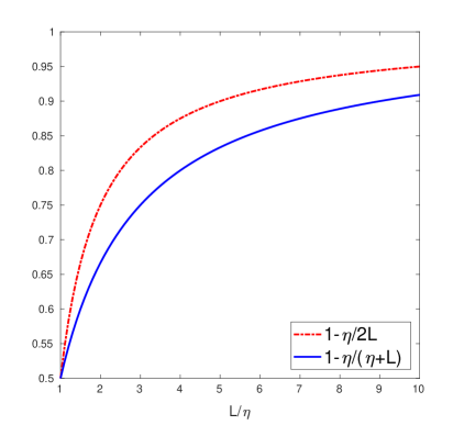
2. Since $L\geq\eta$, it follows that the convergence speed obtained in (30)–(32) is potentially better (specially on ill-conditioned problems) than the optimal one obtained for the SPDG algorithm in [11] via fixed point techniques, namely (16). The same remark applies to the rates in (27)–(29), when compared to the corresponding one in (14). See Figure 1.

3. Note that (31) (resp. (32)) imply that, for a given tolerance $\rho>0$, the SPDG algorithm finds a pair $(x,u)$ (resp. $(x,\gamma y)$) satisfying the termination criterion (11) (resp. $\|{x^{*}-x}\|^{2}+\gamma^{2}\|{u^{*}-y}\|^{2}\leq\rho$) after performing no more than

   $$2+\log\left(\dfrac{\eta+L}{L}\right)^{-1}\log\left(\dfrac{d_{0}^{\,2}}{\rho}\right)$$ (33)

   iterations.

4. By taking $L=57$ and $\eta=9$ (see p. 462 in [11]), we find $\log\left(\dfrac{2L}{2L-\eta}\right)^{-1}\approx 13$ and $\log\left(\dfrac{\eta+L}{L}\right)^{-1}\approx 7$ in (17) and (33), respectively. This shows that the upper bound (33), obtained in this note, is more accurate than the corresponding one (17), obtained in [11].

Figure 1: Solid line: see the convergence rates (30)–(32); dotted line: see (16).

3 Concluding remarks

In this note, we proved that the SPDG algorithm of Mahey, Oualibouch and Tao introduced in [11], can alternatively be analyzed within the Spingarn’s partial inverse framework, instead of the fixed point approach proposed in the latter reference. This traces back to the 1983 Spingarn’s paper, where, among other contributions, he introduced and analyzed the partial inverse method. We simply proved that under the assumptions of [11], namely strong monotonicity and Lipschitz continuity, the Spingarn’s partial inverse of the underlying maximal monotone operator is strongly monotone as well. This allowed us to employ recent developments in the convergence analysis and iteration-complexity of proximal point type methods for strongly monotone operators. By doing this, we additionally obtained a potentially better convergence speed for the SPDG algorithm as well as a better upper bound on the number of iterations needed to achieve prescribed tolerances.

References

- [1] Alghamdi, M. A., Alotaibi, A., Combettes, P. L., Shahzad, N.: A primal-dual method of partial inverses for composite inclusions. Optim. Lett. 8(8), 2271–2284 (2014).
- [2] Alves, M. Marques, Lima, S. C.: An inexact Spingarn’s partial inverse method with applications to operator splitting and composite optimization. J. Optim. Theory Appl., published Online: November 13, 2017 (doi:10.1007/s10957-017-1188-y).
- [3] Alves, M. Marques, Monteiro, R. D. C., Svaiter, B. F.: Regularized HPE-type methods for solving monotone inclusions with improved pointwise iteration-complexity bounds. SIAM J. Optim., 26(4): 2730–2743 (2016).
- [4] Boţ, R. I., Csetnek, E. R.: A hybrid proximal-extragradient algorithm with inertial effects. Numer. Funct. Anal. Optim. 36(8), 951–963 (2015).
- [5] Burachik, R. S., Sagastizábal, C.A., Scheimberg, S.: An inexact method of partial inverses and a parallel bundle method. Optim. Methods Softw. 21(3), 385–400 (2006).
- [6] Ceng, L. C., Mordukhovich, B. S., Yao, J. C.: Hybrid approximate proximal method with auxiliary variational inequality for vector optimization. J. Optim. Theory Appl. 146(2), 267–303 (2010).
- [7] Eckstein, J., Silva, P. J. S.: A practical relative error criterion for augmented Lagrangians. Math. Program. 141(1-2, Ser. A), 319–348 (2013).
- [8] He, Y., Monteiro, R. D. C.: An accelerated HPE-type algorithm for a class of composite convex-concave saddle-point problems. SIAM J. Optim. 26(1), 29–56 (2016).
- [9] Iusem, A. N., Sosa, W.: On the proximal point method for equilibrium problems in Hilbert spaces. Optimization 59(8), 1259–1274 (2010).
- [10] Lotito, P. A., Parente, L. A. Solodov, M. V.: A class of variable metric decomposition methods for monotone variational inclusions. J. Convex Anal. 16(3-4), 857–880 (2009).
- [11] Mahey P., Oualibouch S., Tao P. D.: Proximal decomposition on the graph of a maximal monotone operator. SAIM J. Optim., 5(2): 454–466 (1995).
- [12] Monteiro, R. D. C., Ortiz, C., Svaiter, B. F.: Implementation of a block-decomposition algorithm for solving large-scale conic semidefinite programming problems. Comput. Optim. Appl. 57(1), 45–69 (2014).
- [13] Monteiro, R. D. C., Ortiz, C., Svaiter, B. F.: An adaptive accelerated first-order method for convex optimization. Comput. Optim. Appl. 64(1), 31–73 (2016).
- [14] Monteiro, R. D. C., Svaiter, B. F.: On the complexity of the hybrid proximal extragradient method for the iterates and the ergodic mean. SIAM Journal on Optimization 20, 2755–2787 (2010).
- [15] Monteiro, R. D. C., Svaiter, B. F.: Iteration-complexity of block-decomposition algorithms and the alternating direction method of multipliers. SIAM J. Optim. 23(1), 475–507 (2013).
- [16] Ouorou, A: Epsilon-proximal decomposition method. Math. Program. 99(1, Ser. A), 89–108 (2004).
- [17] Rockafellar, R. T.: Augmented Lagrangians and applications of the proximal point algorithm in convex programming. Math. Oper., 1(2): 97–116 (1976).
- [18] Rockafellar, R. T.: Monotone operators and the proximal point algorithm. SIAM J. Control Optimization 14(5), 877–898 (1976).
- [19] Solodov, M. V., Svaiter, B. F.: A hybrid approximate extragradient-proximal point algorithm using the enlargement of a maximal monotone operator. Set-Valued Anal. 7(4), 323–345 (1999).
- [20] Solodov, M. V., Svaiter, B. F.: An inexact hybrid generalized proximal point algorithm and some new results on the theory of Bregman functions. Math. Oper. Res. 25(2), 214–230 (2000).
- [21] Solodov, M. V., Svaiter, B. F.: A unified framework for some inexact proximal point algorithms. Numer. Funct. Anal. Optim. 22(7-8), 1013–1035 (2001).
- [22] Spingarn, J. E.: Partial inverse of a monotone operator. Appl. Math. Optim. 10(3), 247–265 (1983).