B.S., Yale University (2009) Department of Physics

Doctor of Philosophy in Physics

September 2016 August 26, 2016

Richard MilnerProfessor

Nergis MavalvalaCurtis and Kathleen Marble Professor of Astrophysics
Associate Department Head of Physics

Measuring the lepton sign asymmetry in elastic electron-proton scattering with OLYMPUS

OLYMPUS is a particle physics experiment that collected data in 2012 at DESY, in Hamburg, Germany, on the asymmetry between positron-proton and electron-proton elastic scattering cross sections. A non-zero asymmetry is evidence of hard two-photon exchange, which has been hypothesized to cause the discrepancy in measurements of the proton’s electromagnetic form factors. Alternating electron and positron beams, accelerated to 2 GeV, were directed through a windowless, gaseous, hydrogen target, and the scattered lepton and recoiling proton were detected in coincidence using a large acceptance magnetic spectrometer. Determining the relative integrated luminosity between the electron and positron data sets was critical, and a new technique, involving multi-interaction events, was developed to achieve the desired sub-percent accuracy. A detailed Monte Carlo simulation was built in order to reproduce the convolution of systematic effects at every stage of the experiment. The first stage in the simulation was new radiative event generator, which permitted the full simulation of the non-trivial radiative corrections to the measurement. The analysis of the data and simulation showed that the lepton sign asymmetry rises by several percent between a momentum transfer of 0.5 GeV${}^{2}/c^{2}$ and 2.25 GeV${}^{2}/c^{2}$. This rise as a function of increasing momentum transfer confirms that two photon exchange at least partially contributes to the proton form factor discrepancy.

Chapter 1 Introduction

1.1 The Proton Form Factor Discrepancy

More than a decade ago, a new experimental technique for studying the properties of the proton revealed a glaring inconsistency. The properties of interest were the proton’s electromagnetic form factors, which are a universal way of describing how the proton’s electromagnetic charge and current are distributed within its volume. The proton is a composite particle, made up of many smaller particles and their associated fields. The proton’s positive charge and anomalously large magnetic moment are produced by the arrangement of the proton’s components. Understanding the proton’s form factors, which convey information about this arrangement, has long been a goal of the field of particle physics.

The inconsistency cut between the two experimental techniques for measuring the proton’s form factors. Results obtained with the newer polarization transfer method found different form factors than older experiments using Rosenbluth separation. New Rosenbluth separation experiments, performed as a cross-check, confirmed the discrepancy rather than resolving it. Each technique measures a proton structure that is incompatible with the results of the other.

The leading hypothesis about the cause of this discrepancy is that the results of previous experiments have been distorted by two-photon exchange. Both polarization transfer and Rosenbluth separation rely on elastic scattering between electrons and protons, assuming that, in such reactions, exactly one photon is exchanged between the electron and proton. Reactions in which two (or more) photons are exchanged are neglected when interpreting the results. If two-photon exchange were properly accounted for, perhaps the form factor results might be brought into accord.

Since there is no model-independent theoretical technique for calculating the two-photon exchange contribution, several experiments were conducted to measure it directly. OLYMPUS is one such experiment, and its design, operation, and results are described in this thesis.

1.1.1 Proton Ftructure and Form Factors

Conclusive measurements at Stanford in the 1950s determined that the proton is not a point-like particle [1, 2, 3, 4, 5, 6, 7]. This discovery was monumental, first for exposing a deeper level in the catalog of nature’s building blocks, and second for spawning a field of research dedicated to understanding the proton’s internal workings. The puzzle of proton structure has several difficulties that define it. Unlike in an atomic nucleus, the proton’s constituents (quarks and gluons) are light compared to the binding energy of the system; that is, they are highly relativistic. And, unlike electrons around an atom, the interactions are strong and therefore cannot be understood perturbatively. Calculating the structure of the proton is not yet possible using a fundamental theory. However, there are significant in-roads that can be made with experiments.

One of the important experimental techniques is elastic electron scattering. An accelerated electron is a very useful probe of the interior of the proton because its interactions are primarily governed by quantum electro-dynamics (QED), a theory that is well understood using perturbative techniques. Elastic electron scattering yields information about the electromagnetic charge and current distributions of the proton.

The common formalism for interpreting elastic scattering experiments makes use of structure functions called form factors. A proton’s electromagnetic interactions are different from a point-like electron because the proton’s charge and current are distributed through the proton’s volume. Therefore, it makes sense to modify the proton’s Feynman rules in a general way to account for this difference.

  $$\longrightarrow$$  

Electron vertex function: $$\gamma^{\mu}$$ (1.1)

Proton vertex function: $$F_{1}(Q^{2})\gamma^{\mu}+\frac{i\kappa}{2m_{p}}F_{2}(Q^{2})q_{\nu}\sigma^{\mu\nu}\equiv\Gamma^{\mu}$$ (1.2)

In the above functions, $\gamma$ and $\sigma$ represent Dirac matrices, $q_{\nu}$ represents the 4-momentum carried by the electromagnetic field at the vertex, $Q^{2}=-q_{\nu}q^{\nu}$, $\kappa$ is the anomalous magnetic moment of the proton, $m_{p}$ is the proton’s mass, and finally $F_{1}$ and $F_{2}$ are form factors. The form factors $F_{1}$ and $F_{2}$ are functions of $Q^{2}$. The form factors specify how the complex charge and current distributions of the proton respond to an electromagnetic field. Form factors are the most convenient way for experiments to describe proton structure. They should have definite, universal, values that can be measured by different experiments. But they do, in some sense, obscure what is happening inside the proton at a deeper level. As David Griffiths puts it, using form factors as a way to refer to proton structure “veils our ignorance” [8]. However, the hope is that someday a complete theoretical description of the proton’s internal workings can be used to calculate the values of the proton’s form factors. And until then, models for the structure of the proton can be used to predict values for the form factors, which can then be tested against those measured by experiments.

This expression in equation 1.2 is the most general electromagnetic vertex function for a spin-$\frac{1}{2}$ particle. Therefore, the same language can be used to describe the internal structure of the neutron. The differences in electromagnetic structure of the proton and neutron will be manifest in differences in their respective form factors. For example, the proton has a total electric charge of $+1$ and, as a consequence, $F_{1}(Q^{2}=0)=1$ for the proton. However, for the neutron, a neutral particle, $F_{1}(Q^{2}=0)=0$.

1.1.2 Experimental Techniques for Measuring Form Factors

Figure 1.1: There is one Feynman diagram at leading order for elastic electron-proton scattering.

Using the modified proton vertex function, one can write the matrix element for elastic scattering between an electron and proton (as seen in the Feynman diagram in figure 1.1:

$$\mathcal{M}= \frac{4\pi\alpha}{Q^{2}}\bar{u}(p_{3})\gamma_{\mu}u(p_{1})\bar{u}(p_{4})\Gamma^{\mu}u(p_{2})$$ (1.3)

$$= \frac{4\pi\alpha}{Q^{2}}\bar{u}(p_{3})\gamma_{\mu}u(p_{1})\bar{u}(p_{4})\left[F_{1}(Q^{2})\gamma^{\mu}+\frac{i\kappa}{2m_{p}}F_{2}(Q^{2})q_{\nu}\sigma^{\mu\nu}\right]u(p_{2}).$$ (1.4)

Several observables in elastic scattering reactions can be used to extract the values of the form factors.

Rosenbluth Separation

The basic measurement that can be made using elastic electron scattering is a measurement of the unpolarized differential cross-section. Given the form of the matrix element from above, the resulting lab frame cross section is:

$$\frac{d\sigma}{d\Omega_{e}}=\frac{d\sigma}{d\Omega_{e}}_{Mott}\times\left(\frac{(F_{1}+\tau\kappa F_{2})^{2}}{1+\tau}+\tau(F_{1}-\kappa F_{2})^{2}\left[\frac{1}{1+\tau}+2\tan^{2}\left(\frac{\theta}{2}\right)\right]\right)$$ (1.5)

where $\tau=\frac{Q^{2}}{4m_{p}^{2}}$ [9]. Notice that if $\kappa F_{2}$ were taken to zero and $F_{1}$ to one, then the correction factor would reduce to the expected $(1+2\tau\tan^{2}(\frac{\theta}{2}))$ for electron scattering from a point-like fermion.

Ernst, Sachs, and Wali first identified that the linear combinations of form factors $(F_{1}+\tau\kappa F_{2})$ and $(F_{1}-\kappa F_{2})$ correspond to the electric and magnetic contributions to the cross-section [10]. These combinations are now commonly referred to as the Sachs form factors: the former combination being called the electric form factor $G_{E}$ and the latter the magnetic form factor $G_{M}$. With this substitution and with a little algebra, the cross-section can be rewritten:

$$\frac{d\sigma}{d\Omega_{e}}=\frac{d\sigma}{d\Omega_{e}}_{Mott}\times\left(\frac{1}{1+\tau}\right)\left(G_{E}^{2}+\frac{\tau}{\epsilon}G_{M}^{2}\right)$$ (1.6)

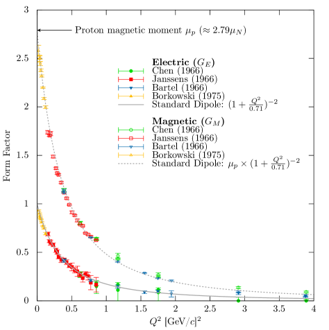
where $\epsilon$ is a kinematic variable defined by $\epsilon^{-1}=1+2(1+\tau)\tan^{2}(\frac{\theta}{2})$. The variables $\tau$ and $\epsilon$ are a linearly independent pair that completely determine the kinematics of the scattering, just like $E_{beam}$ and $\theta$. By measuring the differential cross-section at two values of $\epsilon$ for constant $\tau$, $G_{E}$ and $G_{M}$ can be separated [11]. This technique is called the “Rosenbluth separation” [12], and was used to make the first measurements of the proton’s form factors. From these results, we have a good understanding of the shape of the form factors over a wide range of $Q^{2}$. A sample of early form factor data is shown in figure 1.2.

Figure 1.2: A representative sample of early Rosenbluth separation data is shown [13, 14, 15, 16]. Rosenbluth separation has been used since the 1960s to extract the form factors from cross section data. Both the electric and magnetic have an approximately dipole form: $G\propto(1+\frac{Q^{2}}{0.71})^{-2}$, though the magnetic form factor is scaled higher by a factor of the proton’s magnetic moment, $\mu_{p}$. This suggests that the proton’s charge and current have roughly overlapping spatial distributions. Modern data have revealed small deviations between the form factors and the dipole approximation, and more accurate, albeit more complicated, approximations have been developed.

Methods Using Polarization

The Rosenbluth separation has several drawbacks. The measurement of a cross-section will always have limited accuracy. Large systematic errors come from being unable to perfectly know the acceptance and efficiency of the detectors and luminosity of the experiment. Furthermore, the kinematic factor $\tau/\epsilon$ which multiplies the $G_{M}$ term grows very large at high momentum transfer. Trying to make a Rosenbluth separation at high $Q^{2}$ is nearly impossible because the differential cross-section is dominated by the $G_{M}$ term. The uncertainty in the large $G_{M}$ term drowns out the small $G_{E}$ term.

With the advent of spin-polarized electron beams, two new techniques became possible. In both cases, a longitudinally polarized electron beam is used. The first option is to use a polarized proton target, and to measure the ratio of the transverse single spin asymmetry to the longitudinal single spin asymmetry. The second option is to use an unpolarized proton target, but to measure the polarization of the recoiling proton, specifically the ratio of transverse polarization to longitudinal polarization. In both cases, the result yields the ratio of the form factors.

$$\frac{A_{T}}{A_{L}}=\frac{P_{T}}{P_{L}} =-\frac{G_{E}}{G_{M}}\times\sqrt{\frac{2\epsilon}{\tau(1+\epsilon)}}$$

$$=-\frac{G_{E}}{G_{M}}\times\frac{2M}{E+E^{\prime}}\left[\tan\left(\frac{\theta}{2}\right)\right]^{-1}$$ (1.7)

Practically speaking, recoil polarization measurements are used because it is easier to build a polarimeter with high analyzing power than a target with high polarization, but the two methods are equivalent on theoretical grounds. Polarization experiments are useful not only because their systematic errors are smaller but also because they yield information on the sign of the form factors, not just their squares as in the Rosenbluth separation. Recoil polarization experiments have been used to accurately measure the proton form factor ratio up to a $Q^{2}$ of 10 GeV²/c².

1.1.3 Form Factor Discrepancy

Figure 1.3: ]

Polarization measurements of $\mu_{p}G_{E}/G_{M}$ (red) [14, 17, 18, 16, 12, 19, 20, 21] are inconsistent with Rosenbluth measurements (blue) [22, 23, 24, 25, 26, 27, 28, 29].

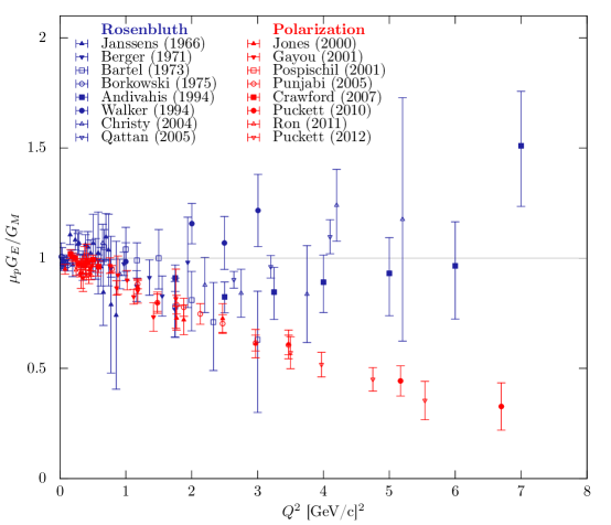
Contrary to expectations, measurements of the ratio $\mu_{p}G_{E}/G_{M}$ from polarization experiments do not agree with their Rosenbluth counterparts. Figure 1.3 shows that the recent measurements of the proton form factor ratio are inconsistent between the two experimental methods. Unpolarized Rosenbluth experiments have measured a form factor ratio that is consistent with unity and is independent of $Q^{2}$. Polarization experiments consistently measure a ratio that falls with increasing $Q^{2}$.

After the emergence of the form factor discrepancy, suspicion was first cast toward the Rosenbluth measurements. In high-$Q^{2}$ measurements the $G_{M}$ term in the Rosenbluth formula dominates the cross section, obscuring $G_{E}$ and leading to large uncertainties. If the uncertainties in old Rosenbluth separation experiments were underestimated, it might be possible that the Rosenbluth and polarization results were consistent after all. However, a new set of Rosenbluth experiments, conducted in the early 2000s, showed results that were consistent with the old Rosenbluth data and inconsistent with the polarization data [20, 21]. Furthermore, the latest polarization experiments reconfirmed the discrepancy [28, 29, 30].

The proton form factor discrepancy clouds our understanding of proton structure. Without its resolution, it is not clear which experimental method, if either, is measuring the true form factors. The effort to find a resolution has prompted a new campaign with both theoretical and experimental efforts, which will be presented in the following chapter. Thus far, the most promising hypothesis is that the discrepancy is caused by hard two-photon exchange.

1.2 Two-Photon Exchange

1.2.1 Theoretical Challenges

The electron-proton cross section presented in section 1.1.2 assumes that the electron exchanges only one virtual photon with the target proton. This assumption makes the calculation far more tractable, and has a tenable justification. Adding an additional photon suppresses the matrix element by a factor of $\alpha$, the fine structure constant. Since $\alpha\approx 1/137$, one can argue that the effect of two-photon exchange should be a sub-percent level correction to the one-photon exchange cross section.

However, a full calculation of the two-photon exchange contribution in a model-independent fashion has not yet been achieved. All calculations so far make some approximation or have some model dependence. One approach is to assume that one of the exchanged virtual photons is soft, i.e. it carries negligible 4-momentum. With this approximation, the one-photon exchange matrix element can be factored out, leaving behind a correction factor. Typically, when experimental data are analyzed, this soft two-photon correction is applied (as part of a standard radiative correction procedure), and any remaining hard two-photon contribution is assumed to be negligible. For this reason, the hypothesized cause of the discrepancy is the hard two-photon exchange, which was not accounted for. Any distinction between hard and soft two-photon exchange is artificial and arbitrary, and is only a result of the approximation that has typically been made during the analysis of previous experiments.

There have been numerous theoretical attempts to calculate the hard two-photon contribution to the electron-proton cross section, and these will be presented in section 2.1. To summarize, there is not a theoretical consensus as to the expected magnitude of the effect. Polarization measurements are probably less susceptible to two-photon exchange, since a ratio of cross sections are being measured; a small correction to both the numerator and denominator is less likely to sway the ratio. Rosenbluth separations, however, which require fitting absolute cross section measurements, are more likely to be affected should hard two-photon exchange contribute significantly to the total cross section.

1.2.2 Experimental Techniques

In the absence of a theoretical consensus, experiments to determine the hard two-photon exchange contribution are needed. Three new experiments recently collected data, and one of those, OLYMPUS, is the subject of this thesis.

The most direct way to measure the contribution from hard two-photon exchange is to look for a lepton sign asymmetry in elastic electron-proton scattering. Any difference between positron-proton and electron-proton elastic scattering cross sections is evidence of two-photon exchange. Furthermore, for two-photon exchange to resolve the form factor discrepancy, the asymmetry must have a specific kinematic dependence, favoring positrons as $Q^{2}$ increases and as $\epsilon$ decreases.

All three contemporary experiments are aiming to quantify the lepton sign asymmetry over a range of kinematic space, though the specific techniques used are all slightly different. If the three experiments have consistent findings, the fact that they all used different techniques will generate confidence in the results. To measure a lepton sign asymmetry, one needs beams of accelerated electrons and positrons and a proton target. One needs a detection apparatus that can distinguish elastic scattering events from inelastic background. And one needs to monitor the relative luminosity between the electron scattering and positron scattering data sets.

1.3 The OLYMPUS Experiment

OLYMPUS is a collaboration of over 60 scientists, from 13 institutions, in six countries. The OLYMPUS experiment took place at the Deutches Elektronen Synchrotron (DESY), a particle accelerator complex in Hamburg, Germany, completing data collection in early 2013. OLYMPUS had a very tight timeline; funding was secured in early 2010, and the start of data collection was in February 2012. In that time window, there was an intense effort to complete all of the necessary preparations. Among the long list of accomplishments were the design and construction of a new windowless hydrogen gas target, the assembly and installation of the detector apparatus, and the writing of custom software needed to operate the equipment and collect the data.

The data collection took place in two running periods, the first in February 2012, and the second in the fall of 2012. Following the end of data collection, the collaboration undertook a survey of all of the detector positions, made a map of the detector’s magnetic field, and then began the process of analyzing the data. The first results from the OLYMPUS experiment are included in this thesis, and will be submitted for publication soon.

In this section, I will introduce the reader to the various aspects of the OLYMPUS experiment, previewing what will be covered in detail in this thesis.

1.3.1 How OLYMPUS Worked

To make a lepton-sign asymmetry measurement, OLYMPUS used alternating electron and positron beams from the DORIS storage ring at DESY. The beams were directed on a stationary proton target, consisting of a tube of hydrogen gas, that was internal to the vacuum of the ring. Elastic scattering events were recorded by detecting the scattered lepton and the recoiling proton in coincidence in a toroidal magnetic spectrometer. The electron beam and positron beam were alternated, approximately once per day, to accumulate an electron data set and a positron data set. The relative luminosity of the two data sets, needed for normalization, was monitored by three independent systems.

1.3.2 OLYMPUS Spectrometer

The main detection apparatus in OLYMPUS was a toroidal magnetic spectrometer. One of the reasons that a tight timeline was possible was that the spectrometer was repurposed from the BLAST experiment spectrometer [31]. The BLAST experiment had a successful run at the MIT Bates Linear Accelerator Center from 2001–2005. OLYMPUS saved a great deal of time, money, and effort, by reusing a proven detector system. Some refurbishment and upgrades were undertaken, so, with those in mind, I will in this thesis refer to the former BLAST spectrometer as the OLYMPUS spectrometer.

The spectrometer magnet, which spanned nearly 4 m wide by 4 m long, by 4 m high, was made up of eight electromagnetic coils, which were arranged around the beamline like the segments of an orange. The two segments in the horizontal plane were instrumented with particle detectors. Drift chambers measured the trajectories of outgoing particles, while walls of scintillating plastic were used to measure the time-of-flight. The particle trajectories curved slightly in the field of the magnet, and the particle’s momentum was inferred from the amount of curvature. OLYMPUS made a coincidence measurement, detecting the scattered lepton in one sector and the recoiling proton in the other. The spectrometer was left-right symmetric; leptons and protons could be detected in either sector. This symmetry was employed in the data analysis to control systematic uncertainties.

1.3.3 Luminosity Monitoring

The relative luminosity between the electron and positron data sets was crucial in making an asymmetry measurement, and so several new luminosity monitors were built specifically for OLYMPUS. Luminosity could be monitored online by integrating the beam current and the approximate target density, but a percent-level asymmetry measurement required more accurate systems. A pair of tracking telescopes was installed along the $12^{\circ}$ scattering angle in order to measure the rate of forward elastic scattering. In addition to the $12^{\circ}$ telescopes, a pair of electromagnetic calorimeters were positioned at approximately $1.29^{\circ}$ to measure the rates of symmetric scattering from atomic electrons in the target. Both systems achieved systematic uncertainties of less than 0.5% in measuring the relative luminosities between running modes.

1.3.4 Analysis Approach

Discriminating elastic scattering events from background was not a significant challenge. By making a coincidence measurement, and measuring the momenta, angles, and flight time of the both the lepton and proton, the kinematics of elastic scattering events were heavily over-constrained. Kinematic cuts were employed to separate most of the background from signal, and the remaining background was estimated and subtracted.

The analysis was neither as simple nor as straightforward as calculating the asymmetry in the detected elastic scattering events. The asymmetry caused by hard two-photon exchange needed to be extracted from asymmetry caused by other sources. As mentioned in section 1.2.1, a set of standard radiative corrections needed to be applied to remove contributions from soft two-photon exchange. These corrections were convolved with properties of the detector, such as resolutions, acceptances, and efficiencies. Our solution for accounting for these convolutions was to simulate everything. We simulated our radiative corrections, using a new radiative event generator, which includes corrections for soft two-photon exchange. We simulated the propagation of these events in the geometry of our detector and produced a full simulated data set. We analyzed the real and simulated data sets with the exact same software. The asymmetry we present is corrected for the asymmetry we found in simulation.

1.4 In This Thesis

This thesis is divided into chapters, which can be read as self-contained descriptions of some aspect of the experiment. In the section, I’ll give a brief preview of each chapter.

In chapter 2, I lay out the scientific motivation for OLYMPUS. I present the various theoretical methods for calculating the two-photon exchange contribution. I also show how the previous asymmetry data are inadequate for determining if two-photon exchange is responsible for the form factor discrepancy. Lastly, I briefly compare OLYMPUS and the two other contemporary asymmetry experiments.

In chapter 3, I give an overview of the OLYMPUS apparatus. Detailed descriptions of the apparatus as well as various component detectors can be found in a variety of other published sources, and I do not aim to exceed any of them. However, I do want to give the reader a chance to get familiar with all of the different mechanical aspects of the experiment while this thesis is open. I try to list, wherever possible, the sources that go into greater detail, so that the curious reader can find them.

In chapter 4, I present the survey of the OLYMPUS magnet, which was undertaken after data collection was complete. I try to give a sense of how we planned and conducted the magnetic field measurements, and how we analyzed the data. This chapter goes into more detail than our recently published article on the same subject [32].

In chapter 5, I present the radiative corrections for OLYMPUS. I try to argue why radiative corrections need to be made by experiments in order for results to be interpreted. Next, I explain what specific corrections need to be made for OLYMPUS. Then I go into detail about the new radiative event generator that we wrote specifically for the OLYMPUS analysis. I conclude with a discussion of our attempts to validate the generator.

In chapter 6, I present an alternate method for extracting luminosity from the symmetric Møller/Bhabha calorimeter (SyMB) data. This alternate method makes use of multi-interaction events (MIEs) and effectively trades precision for a more accurate relative luminosity determination. The MIE analysis was initially pursued as a cross check of the main SyMB analysis, but, over time, proved to be a more robust approach. In this chapter, I show a derivation of the method, estimate its systematic uncertainties, and compare the results to those from the $12^{\circ}$ tracking telescopes.

In chapter 7, I discuss the problem of track reconstruction in the OLYMPUS spectrometer. I explain how the drift chamber data must be processed prior to reconstruction. Next, I address how we identify track candidates using pattern matching, and then fit the trajectories of track candidates using the Elastic Arms Algorithm. I conclude with a discussion of the problem of determining the time-to-distance relationship for the sense wires in the drift chambers.

In chapter 8, I lay out the OLYMPUS analysis framework. I first examine the strategy we used in analyzing the data, including our use of simulation at every stage. I then present the analysis chain, and cover each step taken in processing the data. Finally, I show the approach I used in selecting elastic events and estimating backgrounds.

In chapter 9, I discuss the results of the OLYMPUS experiment. I do a preliminary estimate of the systematic uncertainties. I also compare the results to various predictions and to the results of the other contemporary experiments. These results are some of the first to be publicly released from OLYMPUS, and the reader should understand that they are in preliminary form. That is, they will be superseded by analyses which combine my work with the work of my colleagues and make final estimates of the systematic uncertainties.

1.5 A Remark on Collaboration in This Work

The success of the OLYMPUS experiment was only possible through the hard work of over 60 scientists. There was no shortage of problems to be solved, and the original scientific work I contributed could easily fill a thesis. However, this kind of science does not readily lend itself to the classification of “her work”, “his work”, “my work”, and so on. Almost everything that I accomplished in bringing OLYMPUS to fruition was done either in collaboration with a partner, or by working in a small team, or, at the very least, through solo effort that was guided by frequent discussions with one or more of my colleagues. The topics I choose to cover in this thesis are those where I feel I made the most significant contributions. Because OLYMPUS is the work of of ideas and contributions of many people, I will often use the pronoun “we”, when describing some of my accomplishments. I cannot help it. It really was “we.” There are, however, some cases where I touch on areas of expertise of my colleagues. In those cases, I try to recognize my colleagues’ work explicitly, often to point the reader to a different thesis, where more detail can be found.

Chapter 2 Scientific Motivation

2.1 Calculations of Hard Two-Photon Exchange

Hard two-photon exchange was first suggested as a possible solution to the proton form factor ratio problem in a pair of papers in Physical Review Letters Volume 91, Number 14, in the year 2003. The letter by P. A. M. Guichon and M. Vanderhaeghen [33] suggests a phenomenological approach to describing the effects of hard two-photon exchange, while the following letter by P. G. Blunden, W. Melnitchouk, and J. A. Tjon [34] uses a model-dependent hadronic calculation of the hard two-photon contribution. Both letters point out that a precise comparison of $e^{+}p$ and $e^{-}p$ elastic cross sections is the needed experiment to quantify the two-photon exchange effect.

Guichon and Vanderhaeghen make several points in their work that are relevant to the theoretical discussion. The first is that there is no known model independent way to calculate hard two-photon exchange. Any calculation of hard two-photon exchange will rely upon assumptions which are difficult to validate. Secondly, any model for the two-photon exchange effect must also preserve the linearity of Rosenbluth separations. The Rosenbluth separation technique relies on fitting a line to reduced cross section measurements plotted versus $\epsilon$ (at fixed $Q^{2}$). This linear fitting procedure works over a large range of kinematics, so any model for two-photon exchange which would spoil this linearity can be rejected out of hand. Broadly speaking, this constraint implies that any hard two-photon exchange contribution must be roughly linear in $\epsilon$ as well. Thirdly, they point out that even a small contribution from two-photon exchange can have a large effect on the Rosenbluth form factors, without distorting the polarization result.

In their phenomenological approach, Guichon and Vanderhaeghen demonstrate that the inclusion of hard two-photon exchange results in a third form factor, which they label $F_{3}$. All three form factors become functions of both $Q^{2}$ and $\epsilon$, but, because Rosenbluth data appear linear in $\epsilon$, any $\epsilon$ dependence must be weak. By neglecting any $\epsilon$ dependence in $G_{E}$ and $G_{M}$, they are able to numerically extract the third form factor from fits to existing data. The results imply that a hard two-photon contribution must be on the order of a few percent of the total cross section, and must increase with $Q^{2}$, since the form factor discrepancy is greater at higher momentum transfer.

In their letter, Blunden, Melnitchouk, and Tjon attempt to calculate the two-photon exchange diagram using a hadronic model. The two-photon exchange diagrams (the box, and crossed-box diagrams) are difficult to calculate because they have off-shell proton vertices and an off-shell hadronic propagator. In a hadronic model, one attempts to clear these hurdles by assuming that on-shell vertices are reasonably accurate, and that a propagator can be constructed as a coherent sum of propagators of all of the hadronic states available to the proton. The proton can propagate as a proton, or as an excited $\Delta^{+}$, or in any of the other excited states of the proton. In practice one has to terminate the sum, and in this paper only the proton propagator term is used. The results show that with only the proton term included, the two-photon exchange is sufficient to explain about half of the form factor discrepancy. The authors hope that by including the $\Delta^{+}$ term and further hadronic terms, the discrepancy can be fully explained.

Following these letters, there has been a flurry of papers attempting to quantify the magnitude of the two-photon exchange contribution. Without a model-independent theoretical framework, theorists have followed several different model-dependent approaches, each with advantages and drawbacks. The approaches can be grouped in a few major categories based on the models used: phenomenological models [33, 35, 36, 37, 38, 39, 40, 41, 42], hadronic models [34, 43, 44, 45], partonic models [46, 47, 48, 49, 50], and models using dispersion relations [51, 52, 53, 54, 55], though there are other calculations that defy these classifications [56].

2.1.1 Phenomenological Approaches

Following the initial phenomenological work of Guichon and Vanderhaeghen [33], there have been numerous attempts to extract the two-photon exchange amplitude from existing data. Several works have argued that two-photon exchange can be ruled out from the lack of non-linearities in existing Rosenbluth data [35, 36, 37]. Other studies have extracted values of two-photon exchange that are consistent with a resolution of the form factor discrepancy [39], or at least qualitatively consistent with other two-photon calculations [40], though the results are dependent on the functional form chosen to parameterize the two-photon exchange contribution.

An alternative approach is to attribute the cause of the discrepancy entirely to hard two-photon exchange so as to constrain $F_{3}$ and the asymmetry between positron-proton and electron-proton cross sections. This technique serves as a very useful benchmark for interpreting lepton-sign asymmetry measurements. These phenomenological predictions indicate where measurements would have to fall to fully confirm the hypothesis that two-photon exchange causes the proton form factor discrepancy. Phenomenological predictions [38, 41, 42, 57] that include the latest polarization transfer data [30] predict asymmetries on the order of a few percent. That suggests that OLYMPUS aim for uncertainties at the sub-percent level to definitively confirm the two-photon exchange hypothesis.

2.1.2 Hadronic Calculations

The hadronic calculation in the letter by Blunden et al. [34] was followed by a more detailed paper by the same group [43]. The push was then made to include further hadronic intermediate states other than the proton. The $\Delta^{+}$ state was included in a calculation and surprisingly was found to reduce the contribution from two-photon exchange [44]. The addition of many more higher intermediate states was found to have diminishing effect [45]. Even by including many intermediate states, hadronic calculations still suffer, however, because unknown off-shell form factors are approximated, typically with their on-shell values.

2.1.3 Partonic Calculations

In a partonic calculation, the two photon exchange diagram is broken down into interactions between the photons and individual partons within the proton. The calculation requires a parton distribution function as input. The weakness of this method is that parton distribution data will need to be extrapolated in a model-dependent way to elastic kinematics. Nevertheless, Chen et al. performed a partonic calculation using Generalized Parton Distributions (GPD) taken from Deep-Inelastic Scattering (DIS) data, which they describe in an initial letter [46] as well as in a more detailed paper [47]. The results of the calculations suggest that hard two-photon exchange can “substantially reconcile” [47] the form factor discrepancy. Partonic calculations can be improved by including QCD corrections, by using perturbative QCD (pQCD), although the reliability of these corrections is limited to the kinematic region in which the partons inside the proton are weakly interacting (high energies and large scattering angles.) These pQCD calculations typically use proton Distribution Amplitudes (DAs) as their input. Dmitry Borisyuk and Alexander Kobushkin produced a partonic calculation that can be extrapolated towards hadronic results at low $Q^{2}$ [48]. Nikolai Kivel, working with Vanderhaeghen, performed a subsequent partonic calculation using two different DA models, showing that hard two-photon exchange can substatially alter the slope of a Rosenbluth plot without introducing nonlinearities [49]. Kivel and Vanderhaeghen also introduced a formalism based on Soft Collinear Effective Theory that makes more modest claims [50].

2.1.4 Dispersion Relations

Dispersion relations are useful tools for removing the dependence of off-shell form factors from hadronic calculations. By making use of the unitarity and analyticity of the scattering amplitudes, one can relate the real and imaginary parts of on-shell form factors, circumventing the need to rely on approximations of off-shell form factors. Mikhail Gorchtein performed a calculation at high energies using dispersion relations and found that two-photon effects should play a role at the few percent level at forward angles [51]. Borisyuk and Kobushkin made significant progress using dispersive techniques. Their first calculation showed agreement with earlier hadronic calculations [52]. A subsequent calculation was able to fully remove any off-shell form factors [53]. They also added contributions from the $\Delta^{+}$ intermediate state [54] as well as the P33 partial wave [55]. The general tenor of their results shows a hard two-photon correction that helps resolve the discrepancy.

2.1.5 Criticism of the Two-Photon Exchange Hypothesis

There are calculations that contest that hard two-photon exchange is responsible for the form factor ratio discrepancy. E. Tomasi-Gustafsson et al. have long argued that two-photon exchange would necessarily introduce non-linearities in Rosenbluth data [35, 36, 58, 59]. They suggest instead that the discrepancy might be caused by inadequate radiative corrections, specifically the treatment of bremsstrahlung. In references [58, 59], they develop a formalism calculating multi-photon bremsstrahlung that treats the electron vertex as a composite object QED object (made up of soft photons and $e^{+}e^{-}$ pairs). The momentum distribution of the hard electron within the composite vertex can be described by structure functions governed by the Altarelli-Parisi equations (typically used for partons within hadrons). By implementing a radiative correction based on this formalism, Tomasi-Gustaffson et al. show a modification to the Rosenbluth data that can fully explain the form factor discrepancy without any need for hard TPE.

2.1.6 Outlook

There is not a theoretical consensus on the magnitude of the hard TPE effect. A wide variety of calculations and phenomenological extractions support the hypothesis that hard TPE contibutes significantly to the elastic $ep$ cross section and is responsible for the form factor discrepancy. However these calculations all have model-dependencies and the phenomenological extractions all contain assumptions and approximations. Furthermore, this opinion is not unanimous. A minority view, supported by calculations with the electron structure function formalism, is that hard TPE is negligible and that instead our focus should be improving radiative correction procedures.

This state of discord is a clear call for experimental verification. Experiments that measure the size of the hard TPE contribution can validate or disprove the claim that it bears responsibility for the form factor discrepancy.

2.2 Measurements of Hard Two-Photon Exchange

2.2.1 Lepton-Sign Asymmetry

The most direct technique for measuring hard two-photon exchange is the detection of an asymmetry between the cross sections of $e^{-}p$ and $e^{+}p$ elastic scattering reactions. In the one-photon exchange approximation, there is no asymmetry between the two lepton charge signs. The next-to-leading term, the interference between the one- and two-photon exchange amplitudes, is odd in the sign of the lepton charge. Any lepton-sign asymmetry is proportional to this interference amplitude, seen in equation 2.1.

$$\mathcal{M}= \mathcal{M}_{1\gamma}+\mathcal{M}_{2\gamma}+\mathcal{M}_{3_{\gamma}}+\cdots\mathcal{O}(\alpha^{4})$$ (2.1)

$$\left|\mathcal{M}\right|^{2}= \left|M_{1\gamma}\right|^{2}+2\text{Re}\left(\mathcal{M}_{1\gamma}^{\dagger}\mathcal{M}_{2\gamma}\right)+\cdots\mathcal{O}(\alpha^{4})$$ (2.2)

$$A_{2\gamma}\equiv\frac{\sigma_{e^{+}p}-\sigma_{e^{-}p}}{\sigma_{e^{+}p}+\sigma_{e^{-}p}}\approx\frac{2\text{Re}\left(\mathcal{M}_{1\gamma}^{\dagger}\mathcal{M}_{2\gamma}\right)}{\left|M_{1\gamma}\right|^{2}}+\cdots\mathcal{O}(\alpha^{4})$$ (2.3)

Absolute cross section measurements have accuracy that is limited by knowledge of the detector acceptance. By measuring an asymmetry, the only relative cross section measurements are needed.

A non-zero asymmetry indicates two-photon exchange, but the kinematic dependence of the asymmetry can determine whether or not it is responsible for the proton form factor discrepancy. To bring Rosenbluth measurements into agreement with polarization measurements, the asymmetry must have a negative slope with respect to $\epsilon$. As $\epsilon$ decreases, the asymmetry should grow larger, i.e., the positron cross section should exceed the electron cross section. Furthermore, since the form factor discrepancy grows at large $Q^{2}$, we would expect that the asymmetry also grows with respect to $Q^{2}$. Phenomenological predictions (mentioned in subsection 2.1.1) vary in their estimates, but suggest that an asymmetry that grows to several percent at large angles and low $\epsilon$ would be sufficient to resolve the form factor discrepancy.

2.2.2 Radiative Corrections

Extracting the two-photon exchange amplitude from a measured lepton sign asymmetry is complicated by the problem of radiative corrections. The standard elastic scattering radiative correction procedures all include corrections for soft two-photon exchange, two-photon exchange calculated in the limit that one of the exchanged photons carries infinitesimal momentum, i.e., is soft. Since all previous elastic scattering measurements have accounted for soft two-photon exchange, the form factor discrepancy could only be caused by two-photon exchange, in which both photons carry significant momentum. This additional two-photon exchange is given the appellation: “hard two-photon exchange.” In the standard radiative corrections procedures, hard two-photon exchange is assumed to be negligible.

Measurements of the lepton-sign asymmetry are seeking to quantify hard two-photon exchange. This means that these measurements must correct their results for the effect of soft two-photon exchange, as well as the other radiative effects that enter at order $\alpha^{3}$. Isolating hard two-photon exchange essentially amounts to the problem of disentangling one radiative correction from all of the others. It is a problem that requires careful attention, and, for the OLYMPUS experiment, was a primary concern in the design of our simulation and analysis. The specifcs of the OLYMPUS radiative corrections procedure are described in detail in chapter 5.

2.2.3 Previous Experiments

Figure 2.1: Previous asymmetry data, all from the 1960s, lack the precision to make any significant claims about two-photon exchange.

Figure 2.2: Previous asymmetry measurements were either made at high $\epsilon$ where the asymmetry approaches zero, or at low $Q^{2}$ where the form factor discrepancy is small. The interesting kinematic region, at low $\epsilon$ and high $Q^{2}$ has gone unexplored.

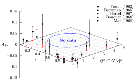
A handful of experiments comparing the cross sections of positron-proton to electron-proton elastic scattering were conducted in the 1960s [61, 62, 63, 64, 65, 66, 67], and their data are shown in the plots in figures 2.1 and 2.2. Some of these results were published in the form of a cross section ratio:

$$R_{2\gamma}=\frac{\sigma_{e^{+}p}}{\sigma_{e^{-}p}}\approx 1+2A_{2\gamma},$$

but for the sake of consistency, I present all of the results re-worked as asymmetries.

In figure 2.1, the data are plotted with respect to $\epsilon$ (upper plot), and with respect to $Q^{2}$ (lower plot). Most of the measurements have uncertainties on the order of 5–10%, making them unable to distinguish between the null hypothesis (hard two-photon exchange is negligible, $A_{2\gamma}=0$) and the alternative hypothesis (hard two-photon exchange resolves the discrepancy: $A_{2\gamma}$ rises several percent with decreasing $\epsilon$ and increasing $Q^{2}$). If anything is to be concluded experimentally about hard two-photon exchange, better data are needed.

A further weakness of these data can be clearly seen by plotting the data over the two-dimension $\epsilon,Q^{2}$ plane, shown in figure 2.2. The specific value of $Q^{2}$ and $\epsilon$ for each data point is marked with a red dot on the plane. The asymmetry value of each point is shown with a black point using the vertical axis. The data largely fall into two groups. Measurements were either made at high values of $\epsilon$, where the asymmetry is theoretically constrained to be close to zero, or the data were measured at small values of $Q^{2}$, where the form factor discrepancy is small. The kinematic region relevant for two photon exchange—where $\epsilon$ is low and $Q^{2}$ is high—is not covered. New experiments are needed to push into this region.

2.2.4 Contemporary Experiments

Figure 2.3: The three contemporary asymmetry experiments push into the high $Q^{2}$, low $\epsilon$ kinematic region. The CLAS experiment does not have a fixed beam energy, so its kinematic reach extends over a large area on the kinematic plane. The shading approximately represents the log of the event rate in CLAS.

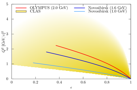
The emergence of the form factor discrepancy, as well as the inadequacy of previous data, prompted the design of three new experiments to measure the lepton sign asymmetry. In addition to OLYMPUS were experiments that collected data in Novosibirsk, Russia, and at Jefferson Lab, in the United States. Both will be described in this section. All three experiments push into the low $\epsilon$, high $Q^{2}$ kinematic region, though all have slightly different coverage, as seen in figure 2.3. The experiments also use different techniques, reducing the susceptibility to a single common systematic error. The results of all three experiments will be discussed in chapter 9.

Experiment at VEPP-3, Novosibirsk

The Novosibirsk experiment collected data in two runs in 2009 and 2012 at the VEPP-3 storage ring in Novosibirsk, Russia [68]. Alternating electron and positron beams were directed through an internal gaseous hydrogen target. Above and below the target were wide-angle non-magnetic spectrometers, consisting of drift chambers for tracking, scintillators for triggering, and NaI crystals for energy measurements. The lepton and proton were detected in coincidence. Combining both runs, the dataset contains almost 1 fb^-1 of integrated luminosity.

The strength of this experiment was its non-magnetic design, ensuring both species of lepton had identical acceptances. This came at the cost of having no momentum analysis for background rejection. A weakness of this experiment was that it depended on forward-angle electron-proton scattering for its luminosity monitoring. Since its luminosity monitoring was susceptible to two-photon exchange effects, the Novosibirsk results quote the asymmetry as being relative to that of the “luminosity normalization point” (LNP). The LNP is at high $\epsilon$ where the lepton sign asymmetry should be close to zero. However, this normalization introduces some degree of uncertainty that makes their results less able to reject hypotheses.

The results from both runs were published in 2014 [68].

CLAS Two-Photon Experiment, Jefferson Lab

The CLAS two-photon experiment at Jefferson Lab (E-07-005) used a much more exotic technique. To avoid the problem of luminosity normalization, they scattered a beam of $e^{+}e^{-}$ pairs on a liquid hydrogen target and collected electron scattering data and positron scattering data at the same time. To produce the beam, they directed the 6 GeV electron beam from the CEBAF accelerator against a gold foil, producing a secondary beam of bremsstrahlung photons. This photon beam was directed against a second gold foil to produce a tertiary beam of $e^{+}e^{-}$ pairs. A tungsten shield blocked any remaining photons, while the electrons and positrons were steered around it by means of a magnetic chicane. The fluxes of electrons and positrons on the target were matched by periodically flipping the chicane polarity.

The experiment used the CEBAF Large Acceptance Spectrometer (CLAS) in Jefferson Lab’s Hall B for its detector. CLAS is a toroidal magnetic spectrometer that has nearly full azimuthal coverage. CLAS has drift chambers for particle tracking inside a layer of scintillator, which measures time-of-flight. A forward electron calorimeter was used for triggering, but not for energy measurements in this experiment. Leptons and protons were detected in coincidence.

A side effect of the pair-produced beam was that the incoming lepton energy was not fixed, but rather varied between several hundred MeV and up to 5.5 GeV. The incoming lepton energy was reconstructed kinematically in each event. Whereas OLYMPUS and the Novosibirsk experiment sample lines of fixed beam energy in the $\epsilon,Q^{2}$ plane, the CLAS experiment samples an area over that plane. Furthermore, the sign of the lepton in any given event was not predetermined. The identification of positrons versus electrons was made using the curvature direction of the tracks.

The strength of this experimental approach is the novel method for handling the problem of luminosity normalization. The weaknesses are the low luminosity afforded by a tertiary beam, and from the systematics associated with the various magnetic fields used in their apparatus. The CLAS two-photon collaboration has not yet reported estimates of the luminosity they collected, but one can estimate, based on the sizes of their statistical uncertainties on their results, that they collected on the order of hundreds of inverse picobarns. Large bins were needed to accumulate enough statistics. Magnetic fields are always a potential source of asymmetry between electrons and positrons, and to limit any false asymmetry, CLAS relied on a complicated protocol for flipping the magnet polarities. Not all magnet polarities could be changed: a mini-torus used for sweeping background from Møller and Bhabha scattering went unflipped. Furthermore, not all of the polarity configurations produced usable data.

The CLAS two-photon experiment collected data in a proof-of-concept run in 2006 [69], followed by a full production run at the end of 2010 and beginning of 2011. Preliminary results have been published [70], and full results have been submitted for publication [71].

Chapter 3 Apparatus

3.1 Introduction

The apparatus of the OLYMPUS experiment was a large-acceptance magnetic spectrometer. Much of this spectrometer was previously used in the BLAST experiment, at MIT-Bates. Some components of BLAST were not needed for OLYMPUS (neutron detectors, for example), and some new components were built specifically for OLYMPUS (most notably, the target and luminosity monitors). OLYMPUS was conducted at the DESY laboratory, in Hamburg, Germany, which meant that the BLAST components had to be shipped from Massachusetts to Hamburg. Shipments arrived in Germany in 2010, and the spectrometer was assembled in a staging area near the storage ring. In July, 2011, the spectrometer was rolled on rails into place, and the ring beam pipe was reconnected. Two periods of dedicated data taking took place. The first was a month of running over February of 2012. The second period was three months of running in the fall of 2012. Cosmic ray data was taken for the first month of 2013. Then the detector and magnetic field was surveyed. In the spring of 2013, the detector was disassembled, and many components were recycled into new experiments.

Figure 3.1: This illustration shows the detectors that make up the OLYMPUS spectrometer. The top four magnet coils are not shown. The scattering chamber is marked by the red oval.

This chapter will describe the various components of the OLYMPUS apparatus as they were used in data collection. An illustration of the spectrometer with the top four magnet coils removed can be found in figure 3.1. Since much of the apparatus was designed for the BLAST experiment, very little of this chapter contains original design work on my part, although I will make a note where it occurs. Instead, this chapter presents the germane information for understanding how the detectors functioned in order to make the lepton sign asymmetry measurement. More detailed information on the apparatus can be found in a couple of published sources. The BLAST technical design report [72] contains a number of specific technical details, but one should exercise caution because it presents a proposal for BLAST, not what was actually built. A more concise article describes BLAST as it was realized [31]. Valuable technical details can be found in a several of the early PhD theses of BLAST students [73, 74, 75]. Finally, at the time of this writing, there have been several articles published with concise technical descriptions of the OLYMPUS apparatus [76] and several of its components [77, 78, 32].

3.2 Accelerator

Figure 3.2: OLYMPUS was assembled in a staging area, and then rolled into place in the south hall of the DORIS ring.

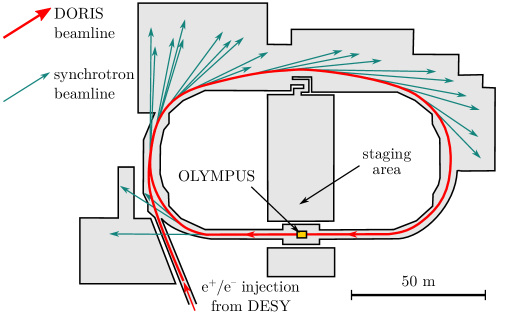
The OLYMPUS experiment was conducted at the DORIS storage ring at DESY, in Hamburg, Germany. The layout of the DORIS ring is shown in figure 3.2. DORIS is a German acronym for DOppel-RIng-Speicher, meaning double-ring store. As its name implies, DORIS was once an $e^{+}e^{-}$ collider, but it was reconfigured several times during its lifetime. In the time leading up to OLYMPUS, DORIS operated primarily as a synchrotron light source. Wiggler magnets and numerous photon beamlines had been installed in curved sections of the ring. In typical running a 4.5 GeV, 140 mA, positron beam was stored in five bunches, providing a steady source of synchrotron X-rays in the photon beam lines. OLYMPUS, by contrast, ran with alternating electron and positron beams of 2.01 GeV and 40–65 mA stored in ten bunches. Running with a greater number of bunches was preferable since it reduced the maximum instantaneous current and reduced the number of random coincidences per unit of luminosity. The current was chosen as a trade-off between luminosity and background rates. A table of the properties of the DORIS ring for OLYMPUS running is shown in table 3.1.

Parameter	Value
Ring circumference	289.193 m
Revolution frequency	1.036652 kHz
Beam energy	2.01 GeV
Beam current	$\approx$ 65 mA
Bending radius	12.18 m
Horizontal emittance	200 nm$\cdot$rad
Vertical emittance	5 nm$\cdot$rad
RF frequency	499.6665 MHz
Harmonic number	482
Bunch spacing	100, 100, 100, 100, 96 ns

Table 3.1: These were the parameters for the DORIS ring during OLYMPUS running.

The DORIS ring could be configured to store either electrons or positrons, and switching between these configurations took approximately one hour. OLYMPUS took data alternating between electron and positron beams, switching between the beam species daily. Counter-intuitively, positron running tended to be more stable. The positive beam repelled positive ions from residual gas in the beam pipe, whereas the electron beam attracted these ions and scattered from them at higher rates. For this reason DORIS operated with positrons when running as a synchrotron light source. Probably the higher reliability for positron running was in part also due to the accelerator operators being more practiced at correcting instabilities in positron mode. Whatever the cause, electron running had perceptibly more frequent high-voltage trips and beam losses.

During the injection of particles into DORIS, the OLYMPUS detectors saw noticably higher rates. For this reason, during injection, a signal was sent to the OLYMPUS data acquisition system (DAQ) to inhibit data taking. Though there were occasional high voltage trips, for the most part the detectors could remain in their powered state through injection. During the February running period, the ring was filled to 65 mA, and then data were collected as the current decayed to 40 mA, at which point the ring was refilled. In the fall run, DORIS was operated in “top-up” mode, in which the ring was filled to 65 mA, and then replenished every few minutes to maintain as constant a beam current as possible.

3.3 Target

A new target system and accompanying beam pipe were designed and built specifically for OLYMPUS and have been described in a recent article [77]. Much of the scientific program at BLAST required spin-polarized targets, so cryogenics, polarimetry, and spin transport were the primary technical concerns. OLYMPUS had no need of spin polarization, but did have to contend with the high bunch-charge in the DORIS bunches, so wake-field suppression and thermal conductivity were significant factors in the target design.

Figure 3.3: The density profile along the length of the target, as reconstructed from tracks in data, shows the characteristic triangular distribution.

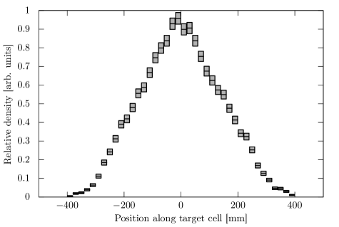
The OLYMPUS target was windowless and internal to the DORIS beamline vacuum. The target itself was a thin aluminum cell, 60 cm long, open at both ends, held inside the beamline vacuum. The beam was steered to pass down the axis of the cell. Hydrogen gas was fed into the cell through a small opening at its midpoint. The gas diffused to the ends of the cell, after which it was removed from the beamline by a system of six turbomolecular vacuum pumps. This windowless design produced a characteristic triangular density profile, shown in figure 3.3.

Figure 3.4: The target cell, collimator, and wakefield suppressors were placed in the vacuum of the accelerator, inside a specially built scattering chamber.

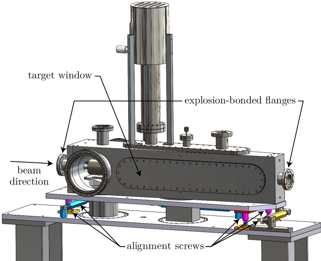
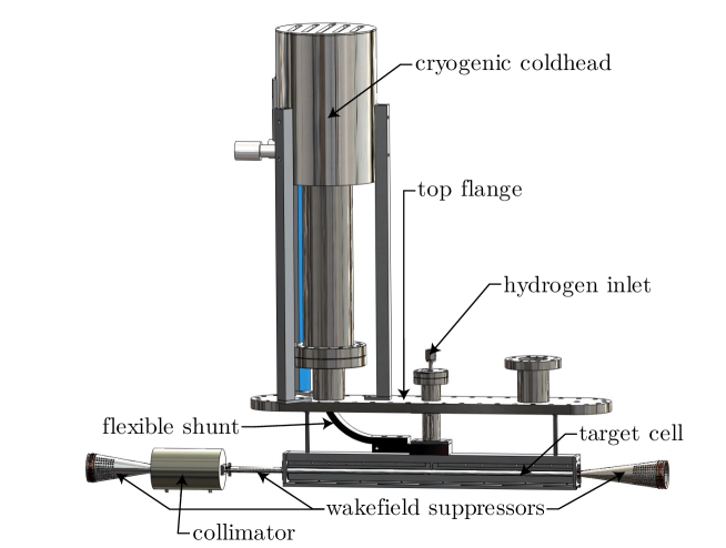
The target was held inside a specially built scattering chamber, which maintained the integrity of the beamline vacuum, but also had thin aluminum windows on either side, to allow scattered particles to pass through without having to traverse a lot of material. An illustration of the scattering chamber and its contents is shown in figure 3.4. The front and back faces had flanges to connect with the up- and down-stream beam pipes. The bottom face had ports for the vacuum pumps, and the top faces had ports for the hydrogen gas, for various sensors, and for a cryogenic coldhead. The coldhead was used to cool the target cell to cryogenic temperatures (in practice, approximately 70 K), and in turn cool the hydrogen gas inside, increasing its density. OLYMPUS aimed to achieve a target density of $3\times 10^{15}$ atoms/cm² without significantly degrading the beam.

A tungsten collimator, 15 cm long and 10 cm in diameter, was positioned just upstream of the target cell in order to protect the thin cell from beam-halo particles and from synchrotron radiation. The target aperture was slightly smaller than the target cell, and was slightly flared downstream to reduce showering and small-angle scattering. The outer dimensions were chosen based on the results of simulated beam-halo showers.

The collimator and target cell were connected to each other and to the upstream and downstream beampipes with conductive metal tubes to suppress wake-fields. Since any sharp transitions between conducting surfaces could be a source of induced wake-fields, these wake-field suppressors were designed to provide continuous electrical conductivity through the entire length of the scattering chamber. The first wake-field suppressor was shaped like a cone, and joined the upstream beamline port of the scattering chamber to the upstream face of the collimator. The second was an elliptical tube that connected the downstream aperture of the collimator to the upstream end of the target cell. The third connected the downstream end of the target to the downstream beamline port of the scattering chamber. The wakefield suppressors had small holes to allow hydrogen gas to pass through them, allowing more efficient vacuum pumping.

The three meters of beamline downstream of the target were also specially designed for OLYMPUS. In addition to large diameter ports for turbomolecular vacuum pumps, the beamline was widened to transmit symmetric Møller and Bhabha leptons to the SyMB calorimeters. In front of the calorimeter apertures, the wide beamline had a cap with three ports. The center port connected to the narrow downstream beamline to circulate the stored beam. The left and right port had thin aluminum windows to allow symmetric Møller and Bhabha electrons to exit the vacuum pipe and enter the calorimeters. This part of the beamline is relevant to the discussion of the luminosity analysis presented in chapter 6, and is shown there as figure 6.1.

The target system had a test run at DORIS in early 2011. The cryogenic and vacuum systems performed well under beam conditions that were to be used for OLYMPUS running. After the test concluded, the target was left in place, without hydrogen gas, for DORIS synchrotron operations. The target could not withstand the higher current synchrotron conditions and had to be removed. It was found that different parts of the target cell frame were made of different types of aluminum, and expanded differently under thermal stress. This caused the cell and frame to deform, which broke the electrical contact of the wake-field suppressors. Subsequent wake-field heating damaged the target cell, and a new cell had to be produced. In this second iteration, 6063 aluminum was used throughout, and the wakefield suppressors were redesigned. The wakefield suppressor connectors were made more robust, and the holes in the wakefield suppressors, necessary for removing hydrogen gas from the target cell, were reduced in number and moved to surfaces that were farther from the beam.

After the conclusion of the February running period, a gap was discovered between the tube that supplied the hydrogen gas to the cell, and the cell inlet itself. Analysis of the luminosity monitor data indicated that only approximately one eighth of the hydrogen was entering the cell; the rest entered the scattering chamber and was removed by the vacuum system. Consequently, the February running period only had one eighth of the expected luminosity. In the summer of 2012, the inlet joint was redesigned to eliminate this gap, and a new target was produced for the subsequent Fall running period. Luminosity monitor data indicated that the Fall target had the desired density and that no gas was leaking from the inlet.

3.4 Magnet

Figure 3.5: The eight coils of the OLYMPUS magnet divided the volume around the beamline into eight sectors, shaped like wedges in an orange.

The magnetic field of the OLYMPUS spectrometer was created by eight electromagnetic coils, arranged like the segments of an orange around the beamline. These coils produced a toroidal magnetic field in the region of the tracking detectors. By measuring the curvature of their tracks, the momentum of charged particles could be inferred. The OLYMPUS magnet was previously used as the BLAST spectrometer magnet, where it was previously described [79].

The OLYMPUS coils were made of hollow copper bars, wound 26 times in two layers of thirteen windings. Each bar was wrapped in fiberglass and then the entire coil was potted in a rigid resin to make the assembly strong enough to resist the strain experienced from magnetic forces. The coils were conventionally conducting, so resistive heat needed to be removed. This was accomplished by flowing cooling water through the hollow recess of each bar. The coils had an irregular shape; the coils were narrower upstream to accommodate the scattering chamber, and then expanded downstream to produce a higher field at forward scattering angles. A photograph of the coils, prior to the installation of the OLYMPUS detectors, is shown in figure 3.6.

Figure 3.6: This photograph shows the magnet coils from the side, prior to the installation of any of the detectors.

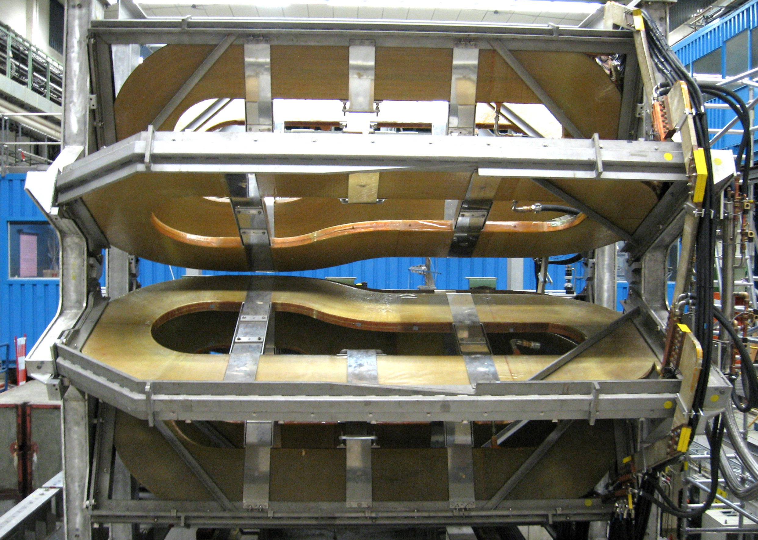
The coils were arranged to produce a toroidal field. The beam passed through the central axis of the toroid, with the target slightly upstream of the center. The field was azimuthally symmetric, which mirrored the azimuthal symmetry of the cross section. The 8 coils divided the region around the target into eight wedge-shaped sectors, each roughly 45^∘ wide. Two of these sectors, the one left and the one right of the target in the horizontal plane, were instrumented with detectors.

At BLAST, the magnet was operated with a current of 6730 A, producing a peak field of approximately 0.4 T. At OLYMPUS, the magnet was operated at 5000 A, producing a peak field of 0.3 T. This naively corresponds to a radius of curvature of 11 m for electrons with 1 GeV/$c$ of momentum. Given a tracking plane spacing $L\approx 0.5$ m, for perpendicular tracks the sagitta $s$ is given by $s\approx L^{2}/2R$, which comes to about one centimeter. Thus, we can expect sagittae on the order of a few millimeters for higher momentum tracks, and sagittae on the order of a few centimeters for lower momentum tracks.

The magnet could be operated with two different polarities, which were referred to as positive and negative, although they represent, respectively, the magnetic field lines pointing counter-clockwise and clockwise around the beamline when facing downstream. It was originally intended that the magnet polarity be flipped every few hours to reduce systematics stemming from electrons and positrons having different trajectories. In the high-luminosity environment of the fall run, negative polarity running had to be abandoned. With negative polarity, low-energy Møller electrons are bent by the magnetic field into the drift chambers, swamping them with noise and current. The schematic in figure 3.7 shows the track curvature produced with positive polarity.

At the conclusion of data taking, there was an intense effort to survey the magnetic field in the volume relevant for track reconstruction. Those efforts were described in a recent paper [32], and are the subject of chapter 4 in this thesis.

3.5 Main Spectrometer

Figure 3.7: This schematic shows an example elastic scattering event for a lepton scattering to the right at an angle of $25^{\circ}$. Both the $e^{-}$ and $e^{+}$ trajectories are drawn in order to show how the magnetic field produces a slight curvature in opposite directions for the two lepton signs.

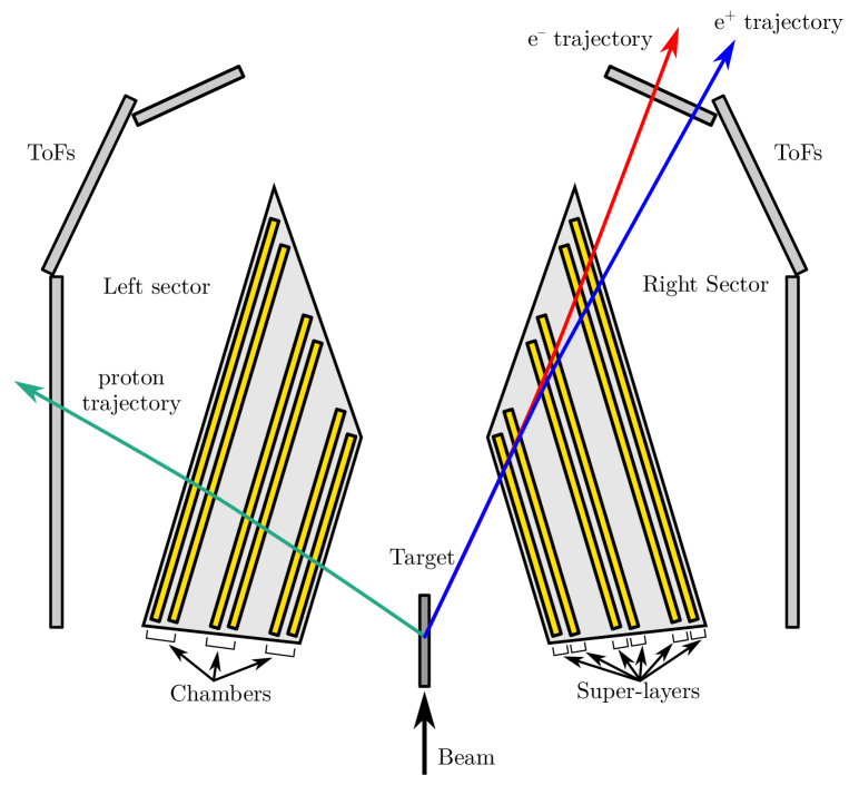
The left and right segments around the target were instrumented with detectors to track scattered leptons and recoiling protons. This system of detectors will be referred to as the “Main Spectrometer” to distinguish it from the 12^∘ luminosity monitors, which also form a spectrometer of sorts. The main spectrometer detectors came from the BLAST spectrometer. Figure 3.7 shows a schematic of an example elastic scattering event in the main spectrometer.

Moving from the target outwards, the first detectors encountered by outgoing particles were a series of drift chambers. These detectors made accurate determinations of the passing particle’s trajectory. This was used to determine the particle’s scattering angle, and, using the curvature caused by the magnetic field, the particle’s momentum. Beyond the drift chambers were the time-of-flight scintillators (ToFs): panels of scintillating plastic which provided accurate timing information. Since these signals could be read out quickly, the ToFs were used to trigger the data acquisition system.

Both of these systems will be described in more detail in the following subsections.

3.5.1 Drift Chambers

The drift chambers were the tracking detectors in the OLYMPUS spectrometer. Drift chambers work by collecting the electrons from ionization of a charged particle passing through a gaseous medium. The passing charged particle will ionize gas atoms along its trajectory. The newly liberated electrons are pulled, using an electric field, to high-voltage wires strung throughout the medium. Close to the wires, the electric field creates an amplification cascade so that a measureable current can be detected on the wire. By measuring the time it takes for the ionization electrons to drift to different sense wires, the trajectory of the particle can be inferred.

Before describing the operational details of the OLYMPUS chambers, I will first describe the layout and introduce the vocabulary that we used to refer to the different parts of the chambers. Some of this vocabulary is shown in figure 3.7. As mentioned earlier, the OLYMPUS spectrometer had two sectors, one to the left and the other to the right of the target. Each sector had its own drift chamber frame: an aluminum trapezoid about the size of a large bathtub. Each frame contained three drift chambers within a single gas volume. The three chambers—the inner, middle, and outer—had wires that were strung nearly vertically from the top and bottom faces of the frame. The inner chamber wires were the shortest, while the outer chamber wires, which were strung at the widest part of the trapezoid, were the longest. Each sector had nearly 5000 wires, of which 477 were read-out.

Figure 3.8: This illustration shows a cross section of a drift cell within a super-layer, looking parallel to the wires, whose cross sections appear as circles. The colors represent the voltage of each wire. The highest voltage wires, the sense wires, attract the ionization electrons produced by nearby tracks. The size of the wires are not to scale.

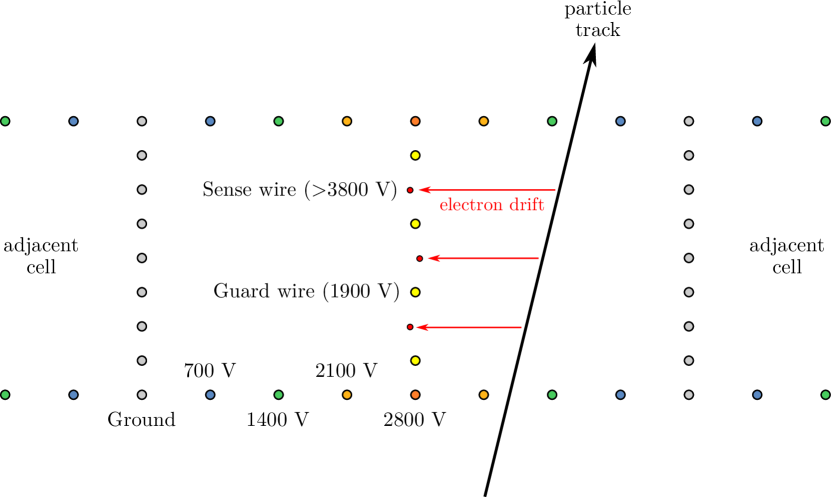
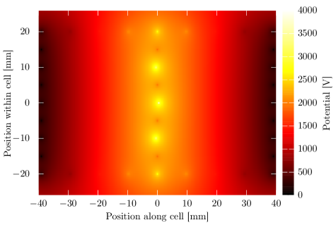
Each chamber was made up of two super-layers, which in turn were made up of rows of a repeated element called a drift cell. A schematic of a drift cell within a super-layer is shown in figure 3.8. Each drift cell was 78 mm long by 40 mm deep, and made up of several dozen parallel wires. The wires were held at specific voltages in order to create a potential gradient across the cell. The wires forming the boundary of the cell were held at ground potential. The center of each cell was held at high voltage. Ionization electrons produced in the cell would drift toward the high voltage wires at the center of the cell. A calculation of the potential within a drift cell is shown in figure 3.9. The number of drift cells in each super layer is shown in table 3.2.

Figure 3.9: The potential is highest at the center of the drift cell, and decreases uniformly to the cell edges.

Chamber	Cells in inner super-layer	Cells in outer super-layer
Inner	18	19
Middle	26	27
Outer	34	35

Table 3.2: The trapezoidal shape of the chambers necessitated more cells per super-layer moving outwards from the target.

Only three of the wires at the center of the cell were read out, called the sense wires. These wires were smaller (only 25 $\mu$m in diameter, compared to 100–150 $\mu$m for the other wires) in order to create larger electric fields and a greater amplification in their vicinity. The sense wires carried the highest potential in the drift cell; they were held typically between 3800 V and 4000 V, balancing signal efficiency with the possibility of sparking.

The arrival times of the ionization electrons at the three sense wires provide information about the track position, but there is an ambiguity about the direction of drift. Given an arrival time, the track could either have originated to the left of the sense wire, or to the right. To resolve these ambiguities, the sense wires are staggered by $\pm 0.5$ mm relative to the high voltage plane. With staggered wires, the ambiguity can be resolved because the correct side will be a better fit to the three arrival times.

The arrival times provide information about the track position perpendicular to the wire, but no information about the position of the track in the direction parallel to the wire. For this reason the wires of each super-layer were rotated $\pm 5^{\circ}$ relative to vertical. Adjacent super-layers had a $10^{\circ}$ stereo angle between them, enough to localize the position of a track in two dimensions.

Refurbishing the Chambers at DESY

After the conclusion of the BLAST experiment, the drift chambers sat idle for several years and, by the time of OLYMPUS, were in need of refurbishment. It was deemed too great a risk to ship them while fully strung. The wires collectively (nearly 5000 per sector) exert significant tension on the frames. It was feared that if many wires broke during shipping, this might initiate a catastrophic failure that could damage the frames. The chambers were unstrung at MIT Bates Laboratory, and then shipped to DESY in the spring of 2010. Over the summer of 2010, both sectors were completely restrung by me and several others in a clean room at DESY. In January of 2011, new electrical connections were soldered to the newly strung wires. In the spring of 2011, the chambers were taken to the DORIS staging area and installed on the OLYMPUS subdetector frames.

In addition to new wires, new high-voltage distribution boards were designed for OLYMPUS. The first iteration was beset by sparking problems: traces carrying several thousands volts passed too closely to ground lines. Despite efforts to insulate the boards with insulating acrylic, spray-on plastic, and RTV silicone, a second iteration of boards was needed. These were rapidly produced at the end of 2011, and installed just before the start of the February run in 2012.

Read-Out Electronics

Several steps of electronic processing are needed to transform current pulses, produced by ionization electrons arriving at a sense wire, into a time signal. The first step is to transform the current pulse into a voltage pulse, which is done by a capacitive circuit on the high-voltage distribution board. Common-mode noise between the sense wire and the adjacent wires (called guard wires) is also removed at this stage. The voltage pulse is amplified by a fast amplifier then sent to a discriminator to be turned into a digital pulse. The digital pulse is sent to a time-to-digital converter (TDC), operated in common stop mode. The wire chamber signal provides the start, and the stop is provided by a trigger signal that has been delayed by a fixed amount of time that is longer than the maximum drift time in the chambers. This arrangement produces the counter-intuitive situation where longer drift times are represented by smaller output times on the TDC. The time of zero-drift was calibrated for each wire.

Time-to-Distance Functions

Analyzing drift chamber data requires converting times from the TDCs to distances between a track and the sense wires, a problem which we gave the name “time-to-distance” or “TTD”. The track reconstruction works best when its internal time-to-distance function is as close as possible to the inverse of the true “distance-to-time” function for the chambers. Developing a good time-to-distance function for the track reconstruction was one of the major analysis hurdles that had to be cleared. To give the reader a sense of scale for the subsequent discussion, an ionization electron could drift the 39 mm from the ground plane to the high-voltage plane in 1–2 $\mu$s.

The drift cells were designed to make the time-to-distance relationship as linear as possible. The electric field is roughly constant in the cell volume, and points from the ground plane to the high-voltage plane. But the field close to the sense wires is much higher than in the bulk, and so, in the region of small times, the function is non-linear. As well, in the region close to the ground plane, ionization electrons feel very little field, and can drift very slowly for hundreds of nanoseconds, before they enter the high-field region and get pulled toward the high voltage plane. This produces a plateau in the time-to-distance function for large times.

To further complicate matters, the time-to-distance function depends on the incidence angles of the track, as well as the local magnetic field. The Lorentz force of a magnetic field has the effect of changing the drift direction of the ionization electrons. Rather than drifting along the electric field lines, the electrons will drift at an angle, called the “Lorentz angle”. Since the toroidal field is non-uniform, every cell has a slightly different Lorentz angle, and requires a slightly different time-to-distance function.

After trying many different approaches, we settled on a simple parameterization that captured the linear-region, the non-linear behavior for very short and very long times, the dependence on incident angles, and the Lorentz angle. We then iteratively fit the parameters for each wire to trajectories found by the track reconstruction software. After several iterations, a set of best-fit parameters was found.

Gas Mixture

The specific gas mixture used in a drift chamber can greatly affect the chamber performance. We made several mistakes with regards to our gas mixture, and I want to discuss those here in the hope that the reader may avoid similar mistakes. First, I remind the reader that typically a mixture of two gases is used; a drift gas which makes up the majority of the mixture, with a small amount of a quench gas. The drift gas should have a low affinity for electrons. The quench gas should have many rotational and vibrational modes in order to absorb photons released during amplification, so as to prevent re-ionization.

At BLAST, a mixture of 82.3% helium (drift gas) and 17.7% isobutane (quench gas) was used [74]. Using isobutane at DESY would have required the hassle of additional safety protocols because of its flammability, so the gas mixture at OLYMPUS was switched to 90% argon (drift gas) and 10% carbon dioxide (quench gas). Both were inert and could be used safely. However, the drift velocity of electrons in the two mixtures were significantly different. Whereas at BLAST, electrons drifted at approximately 20 mm/$\mu$s [73], at OLYMPUS, the drift velocity was closer to 30 mm/$\mu$s. This substantially reduced the position resolution of the drift chambers and even made it difficult to resolve the $\pm 0.5$ mm staggering of the sense wires. Since the staggering was necessary to resolve left/right ambiguities in tracks, track reconstruction became an enormously difficult enterprise.

This was not our only lapse in judgement when it came to the gas mixture. At the beginning of the fall run, one of the problems with the drift chambers was “ringing”: TDC times that appeared to be the result of noise, but were also correlated with the trigger, and spaced an even 100 ns apart. To combat this ringing, we added a small amount of ethanol vapor to the gas mixture. Ethanol is a very effective quench gas, and so it was hoped that a small amount of ethanol might eliminate the ringing. However, the addition of ethanol ended up causing more problems than it solved.

First, it is possible that the gas mixture had nothing to do with the ringing noise. The source of the ringing was never conclusively determined, but with the benefit of hindsight, I suspect that the majority of this noise was caused by background particles produced by the beam (or beam halo) that caused additional ionization in the drift chambers. That would explain the time correlation with the trigger (which was itself, correlated in time with the beam bunches), and the 100 ns time spacing (which is the same as the DORIS bunch spacing). It also explains why this noise was less of a problem in February run. At that time, due to the leak in the target inlet, the target density was lower. This would have reduced the beam halo from beam-target interactions. If this hypothesis is correct, the gas mixture was unrelated to the ringing, and the ethanol might have been a needless complication.

Figure 3.10: The ethanol concentration was not stable, causing the drift velocity to vary over time. The change in drift velocity was so great that it alerted us on two occasions that the ethanol bubbler had become empty.

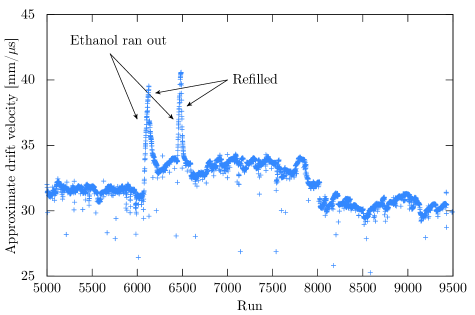
Second, in our hurry to add the ethanol, we did not come up with a mechanism to accurately control the amount of ethanol we added. We passed the dry gas mixture through a liquid ethanol bubbler, which we put in a small refrigerator. The ethanol added to the gas was controlled only by the temperature of the refrigerator. It was clear that the refrigerator temperature varied, we could see changes over time in the drift velocity, shown in figure 3.10. In fact, we could even tell, from the drift velocity alone, when the bubbler ran out of ethanol. The consequence of this temperature variation was that we had to produce different time-to-distance functions for different periods of time during data taking. And since we were never quite sure of the exact proportion of ethanol vapor, we had enormous trouble trying to calculate the drift properties of the gas.

Third, we subsequently learned that we had misunderstood how ethanol is commonly used in drift chamber noise reduction. According to Particle Detection with Drift Chambers by Blum, Riegler, and Rolandi [80], ethanol is often temporarily introduced to chambers that use hydrocarbons (like propane or butane) as their quench gas. In these gas mixtures, the hydrocarbon molecules will adhere to the wires over time, forming long chains or “whiskers”. As these whiskers get longer, they can be source of noise and dark current. Introducing ethanol vapor can help break up these whiskers, restoring the chambers to optimal conditions. However, Blum et al. suggest that ethanol should be periodically added during breaks in operation and then removed, not introduced as a permanent fraction of the gas mixture. In the case of our drift chambers, we were never at risk of whisker growth, given that our quench gas was carbon dioxide, and because we left the ethanol in the chambers during data taking, it substantially altered the drift chamber performance.

3.5.2 Time-of-Flight Scintillators

Figure 3.11: This photograph shows the right sector ToFs when the spectrometer was being assembled in the staging area.

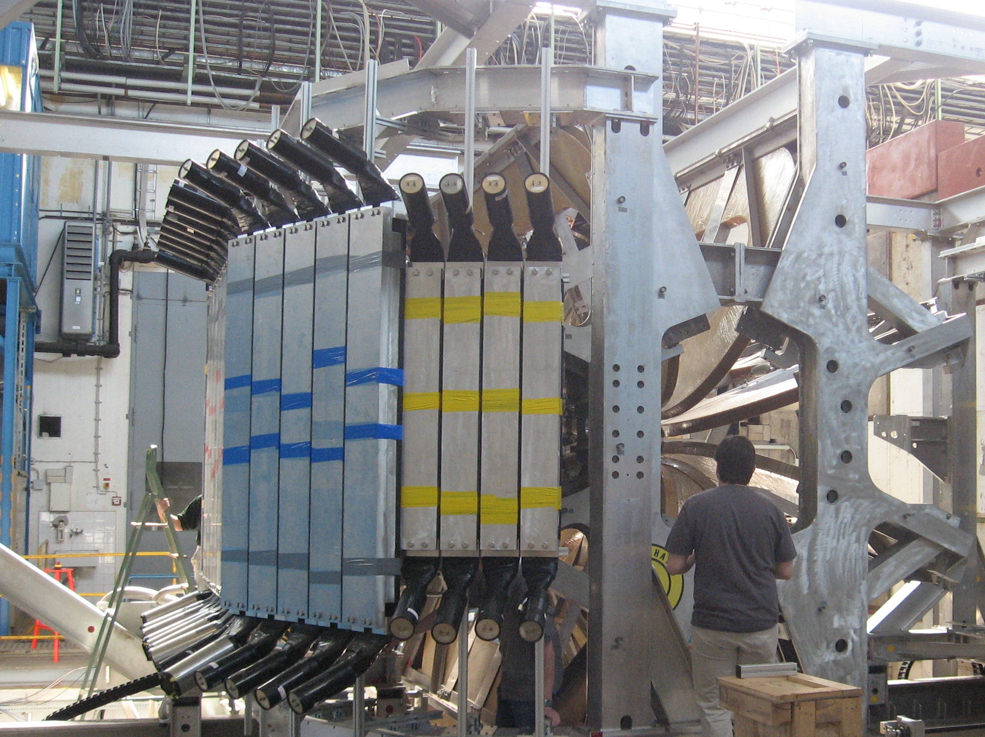
The Time-of-Flight (ToF) scintillators were bars of scintillating plastic that were arrayed in panels outside of the drift chambers. The scintillation light was detected by photo-multiplier tubes (PMTs) attached to the top and bottom ends of each bar. Because the signal and readout from the ToFs was fast, the ToFs were used for timing and triggering. Each sector had three panels for the downstream, middle, and upstream regions of the acceptance. The downstream bars were slightly smaller: 120 cm tall, 17.8 cm wide, and 2.54 cm deep. The other bars were 180 cm tall, 26 cm wide, and 2.54 cm deep. Each sector had a total of 18 bars. Figure 3.11 shows the ToF bars on the right sector.

Each scintillator was wrapped in reflective foil to keep light from escaping. A thin sheet of lead was placed on the face of the bar that faced the target to block low-energy electrons. Plastic light guides were glued to the top and bottom faces. PMTs were positioned flush to faces of the light guide, and coupled with optical grease. The entire assembly was wrapped in black plastic to form a light-tight seal. The PMTs were also wrapped with a layer of Mu-metal to shield them from the magnetic field.

The output from each PMT was split and sent to both an amplitude-to-digital converter (ADC) to record the signal amplitude and to a TDC to record the signal time. The signal amplitude contained information about the light produced by the passing particle, and thus the energy loss, $dE/dx$, though this had to be unfolded from the amount of attenuation that occurred between the track and the PMTs. The mean of the signal times from the two PMTs could be used to determine the time of flight for the particle. The time difference between the two PMTs indicated the track position along the bar. The analysis of the ToF data was performed by my colleagues Lauren Ice and Rebecca Russell, whose recent thesis describes the analysis in more detail [81].

3.5.3 Trigger

The main spectrometer was triggered using a combination of ToF and drift chamber information. The level 1 trigger, which needed to be fast, made use only of ToF information. In each sector, the top and bottom PMTs of a single bar needed to have a signal in coincidence. Furthermore the left sector bar and right sector bar needed to be a specific combination that was possible for an elastic $ep$ scattering event. The background rates of the most downstream ToF bars were very high, and by requiring a valid kinematic combination, a background signal in a left downstream bar and a background signal in a right downstream bar would no longer create a trigger. For scale, the trigger rate was on the order of several hundred Hz, while we estimated the rate of elastic $ep$ events to be on the order of about 10–20 Hz.

In the Fall run, the luminosity increased, and so a second level trigger was developed, which used information from the drift chambers. For the second level trigger to fire, each sector had to have at least one signal from a wire in either the middle or outer chambers. Even this minimal requirement reduced the trigger rate to acceptable levels.

In addition to the main trigger, a number of more permissive test triggers were included, but heavily pre-scaled. These were useful in studying aspects of the detector performance, for example, the ToF efficiencies [81].

3.6 Luminosity Monitors

Figure 3.12: The $12^{\circ}$ telescopes and the symmetric Møller/Bhabha calorimeters were positioned downstream of the scattering chamber.

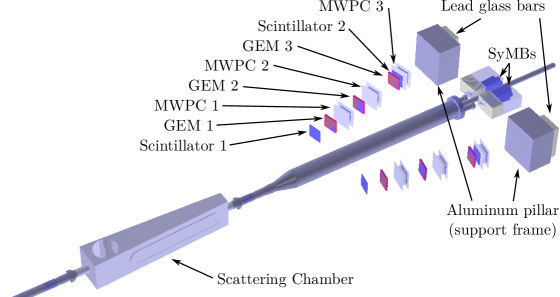
In order for the data from electron running to be compared to that from positron running, the relative luminosity of the two data sets was needed. A rough estimate of luminosity could be made online using the beam current, the target flow rate and target temperature, but for a percent level asymmetry measurement, highly-accurate luminosity monitors were needed. Two independent systems, the $12^{\circ}$ telescopes and symmetric Møller/Bhabha calorimeters (SyMBs), were specially built for OLYMPUS and will be described in this section. A schematic showing their position relative to the downstream beamline can be found in figure 3.12. A description of the luminosity analysis can be found in chapter 6.

3.6.1 $12^{\circ}$ Tracking Telescopes

The $12^{\circ}$ tracking telescopes were a set of tracking detectors positioned along the $12^{\circ}$ scattering angle from the target. Two telescopes were built, and installed in each sector, mounted to the downstream face of the drift chamber frame. Figure 3.12 shows the different detector elements in the telescopes and their positioning relative to the beamline. Each telescope had two planes of scintillator, three gas electron multiplier (GEMs) detectors, and three multi-wire proportional chambers (MWPCs). The scintillators were read out using silicon photomultipliers (SiPMs) and were used to trigger the telescopes. The GEMs and MWPCs were the tracking detectors; they could record the position of a passing charged particle in two dimensions. The position resolution of the MWPCs was on the same scale as the 1 mm spacing between the wires. The GEM detectors had a much finer position resolution of approximately 100 $\mu$m. There was substantial magnetic field in the volume of the telescopes, so a momentum measurement of passing particles could be made.

The $12^{\circ}$ monitored luminosity by measuring the rate of elastic $ep$ scattering in which the lepton passed through the telescope, with an approximately $12^{\circ}$ scattering angle. The recoiling proton would pass through the opposite sector of the main spectrometer. The system was triggered by the coincidence of signals in both telescope scintillators and in both PMTs of an opposite sector ToF bar. For most (about 90%) leptons that passed through the telescopes, the proton also passed through the drift chambers, though this was not required for the trigger. The telescope trigger efficiency was tested using a pre-scaled secondary trigger which only required a signal in bars of scintillating Pb glass, placed at the downstream end of the telescopes. The only convenient way to mount them in position was to strap them to aluminum pillars that served as part of the support frame for the toroid magnet. This meant that passing particles lost some of their energy traversing the pillar, but this was not a problem for a simple trigger test.

An analysis of the $12^{\circ}$ telescope data was performed by my colleague Brian Henderson, and the reader is encouraged to see his thesis for details [82]. The results are also summarized in section 6.1.2.

3.6.2 Symmetric Møller-Bhabha Calorimeters

The symmetric Møller-Bhabha calorimeters (SyMBs) were a pair of lead fluoride (PbF₂) Cherenkov calorimeters, that were positioned 3 m downstream from the target, very close to the beamline, as can be seen in figure 3.12. An article describing the design and operation of the calorimeters was recently published [78]. The calorimeters monitored luminosity by measuring the rate of scattering from atomic electrons in the hydrogen gas of the target—Møller scattering during electron running, and Bhabha scattering during positron running. The calorimeters were positioned at the symmetric scattering angle, in which both final state leptons emerge at the same angle, one entering the left calorimeter, the other entering the right. This angle is approximately $1.29^{\circ}$ for a beam energy of 2.01 GeV.

Each calorimeter was made up of nine lead-fluoride crystals, arranged $3\times 3$, each connected to its own PMT. SyMBs sat in a region of weak magnetic field, and so the entire apparatus—crystals and PMTs—were placed in a mu-metal box, shielding the PMTs from the field. The calorimeter aperture was defined by a collimator: a block of lead with a cylindrical hole. The collimator was positioned in front of the central crystal in the calorimeter. The central crystal contained the bulk of the electromagnetic shower—the crystals were approximately 25 mm in width, and the Molière radius for lead fluoride is 21.24 mm.

The SyMBs had to withstand high rates, on the order of hundreds of kHz. Rather than being read out by the main OLYMPUS data acquisition system (DAQ) every time the SyMBs recorded a signal, the SyMBs had their own data acquisition system. The energy deposited in each calorimeter was recorded in several fast histogramming cards, which could be operated with essentially zero dead time. The histogramming cards could be filled faster than the DORIS bunch frequency, i.e., the SyMBs could distinguish and record signals from adjacent bunches. The histograms were periodically written to the main OLYMPUS DAQ data stream. This meant that event-by-event information was not recorded; only the aggregation of events between readouts was recorded.

The analysis of the SyMB data was undertaken by my colleague Colton O’Connor, and the interested reader should consult his thesis for the most detailed description of that work [83]. Unfortunately, a luminosity extraction directly from Møller/Bhabha scattering rates ended up not being possible, due to large systematic effects that which were not fully considered when the SyMBs were designed. Fortuitously, a secondary analysis, based on the rates of multi-interaction events, turned out to be a much better way to extract luminosity from the data. This analysis is the subject of chapter 6.

3.7 Survey

Many of the detectors described in this chapter were used to make precise measurements of the position of particle tracks. These position measurements were only as accurate as our understanding of where the detectors were physically positioned in space. For this reason, at the end of data taking, a survey of all of the detectors was undertaken. This work was largely performed by the DESY survey group MEA 2.

The survey group used theodolites with laser range-finders to measure the three-dimensional position of special reflective targets. These survey targets were affixed to the walls of the experimental hall (to provide a global reference frame), to parts of the OLYMPUS frame (to provide local reference systems), and to known fixed positions on all of the OLYMPUS subdetectors. The first stage of the survey was conducted in the experimental hall, with the OLYMPUS detector unmoved. Once the position of the OLYMPUS frame within the hall was established, the two sectors of the main spectrometer (and including the $12^{\circ}$ telescopes, which were mounted to the drift chambers) were disconnected, and carried by crane into the staging area. The second stage of the survey was to measure the positions of the drift chambers and ToF scintillators with respect to the subdetector frames. With the ToFs and drift chambers out of the way, a third stage of surveying was possible back inside the experimental hall. There was now an unobstructed view of the scattering chamber, the SyMBs and elements of the beamline. After this was complete, the magnetic field was also surveyed, and this will be described in detail in chapter 4.

The analysis of the survey data was performed by my colleague Jan Bernauer. Jan had to integrate over 5000 position measurements from dozens of reference frames to produce the most likely three-dimensional coordinates for all of the survey targets. He then had to combine these coordinates to estimate the positions and orientations of all of the elements in the OLYMPUS apparatus. This was information used by Colton O’Connor to make a digital map of the apparatus geometry, written in the mark-up language GDML [84]. This map was used at many stages in the analysis: by the simulation’s event generator to place events relative to the beam position monitors, by the simulation’s propagator when simulating trajectories, and in the track reconstruction.

Chapter 4 Magnetic Field Survey

4.1 Introduction

The OLYMPUS spectrometer is a magnetic spectrometer; it uses a magnetic field to transform a charged particle’s momentum information into position information, which can be measured accurately. For this system to work, the magnetic vector field needs to be known throughout the spectrometer volume. Without a magnetic field map, particle tracks cannot be simulated and tracking software cannot determine a track’s momentum. Furthermore, the magnetic field bends electrons and positrons in different directions. Inaccuracy in a magnetic field map can lead to systematic differences between the two lepton species.

The magnetic field could, in principle, be calculated from current in the toroidal magnet and from the shape of the coils. In practice, this was not feasible because of uncertainty in the true positions of the coils. The coils deformed slightly under the strain of magnetic forces when the magnet was powered. Furthermore, the current-carrying copper bars in each coil, described in section 3.4, were potted together with epoxy during construction. Even if we had a perfect survey of the exterior of the coils, we would not know, with high accuracy, where the bars physically sat within the epoxy potting.

A further risk with trying to calculate the field comes from the fact that our field is non-uniform. There are areas of low-field (around the beamline) and high-field (around the drift chambers) and large gradients between them. Slight inaccuracies in the assumed positions of the coils can thrown off the field dramatically, especially in the high-gradient regions.

Rather than calculating the magnetic field, we attempted to measure it. Using a Hall probe positioned by a system of mechanical translation tables, we measured the magnetic field at over 36,000 positions in and around the spectrometer. We analyzed the resulting data to produce a software map that could estimate the field as a function of position, esentially interpolating between measurement positions. This map is used in analysis (specifically by the Geant4 path-swimming routines) to solve the trajectories of charged particles moving through the spectrometer.

A recently-published paper has a concise description of the OLYMPUS magnetic field measurement and data analysis [32]. In this chapter, I’ll try to provide a more detailed account of our efforts and our decision making. I’ll start with an explanation of our measurements, including a description of the apparatus and our procedure. Next I’ll describe how we analyzed the data from these measurements to produce a magnetic field map. Then I’ll show how we used spline interpolation on a precomputed grid to provide the speed up necessary for large-scale simulations. I’ll conclude with some reflections about what would have made our magnetic field measurement better.

4.2 Measurements

4.2.1 Overview

The measurements of the magnetic field were made using a three-dimensional Hall probe, which provided the full magnetic field vector at the probe’s position. The probe was moved through the spectrometer volume by a system of translation tables. Early on in the measurement process, it was discovered that the tables did not provided the desired millimeter-level accuracy in their movements. To correct for this, we used theodolites to determine the probe position.

The measurements were conducted in the spring of 2013, at the conclusion of the OLYMPUS detector survey. The detectors had been removed from the magnet, giving the Hall probe unobstructed access to the spectrometer volume. The apparatus was first assembled on the left side of the magnet to survey the left sector. Then it was taken apart and reassembled on the right side of the magnet for the right sector survey. The process was completed in about four weeks, and over 36,000 field measurements were made.

4.2.2 Apparatus

Figure 4.1: The magnetic field measurement apparatus used a system of translation tables to move the Hall probe to various positions within the spectrometer. This schematic shows the system when set up to measure the left sector.

Figure 4.2: This photograph shows a magnetic field scan in progress on the left sector. The probe is just to the left of the diamond-shaped survey target.

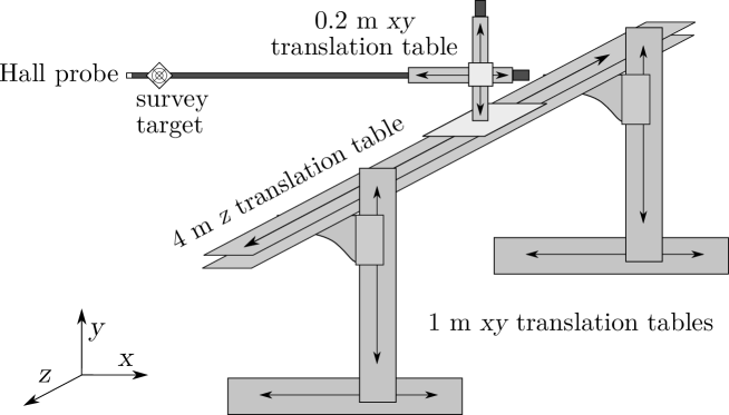
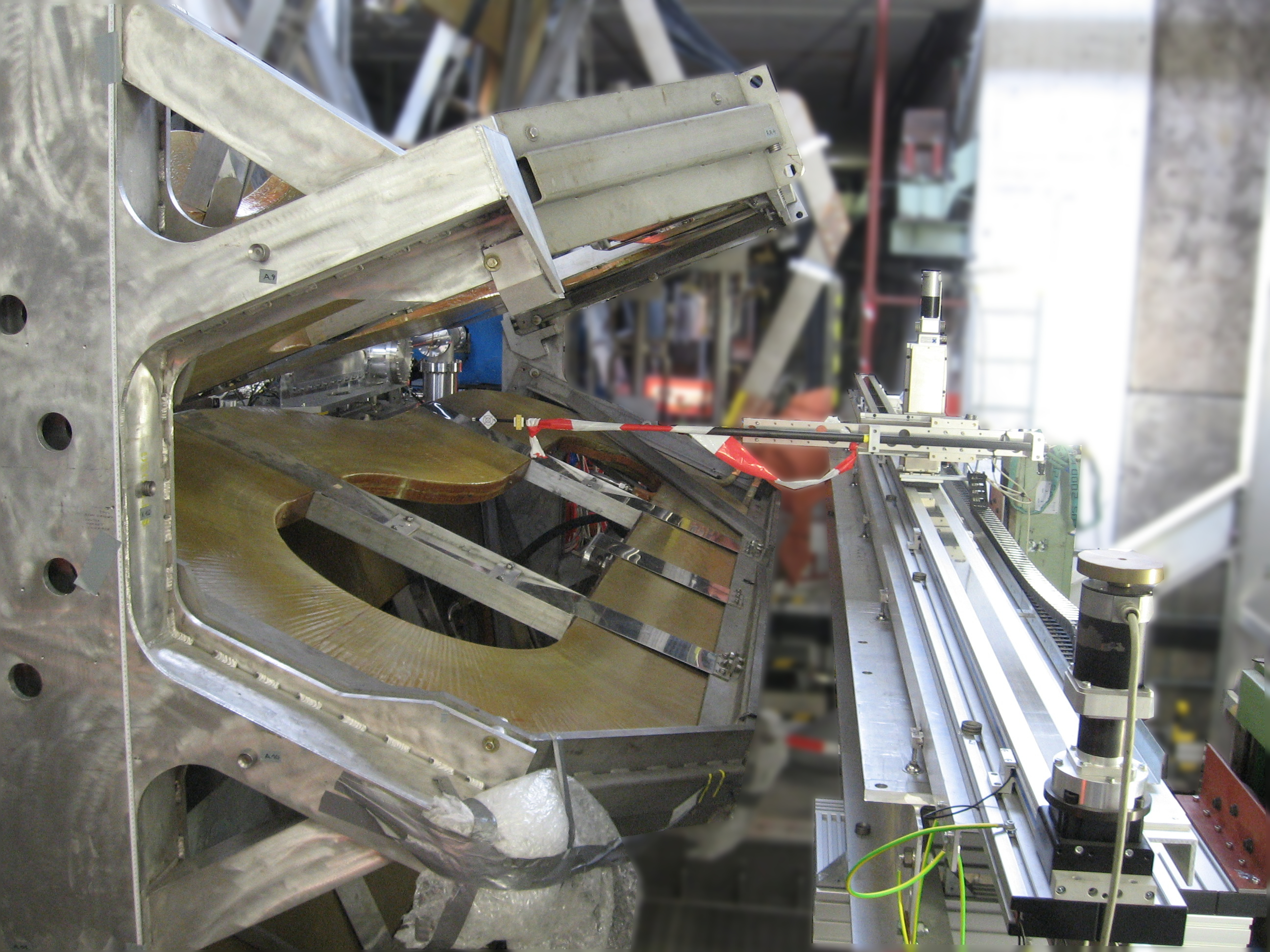
The magnetic field measurements were made using a 3D Hall probe, moved by a system of translation tables. This set-up, a schematic of which is shown in figure 4.1, was originally built for a survey of the undulator magnets of DESY’s free-electron laser FLASH [85]. The base of the apparatus was a pair of translation stands with 1 m range in both the $x$ and $y$ directions. These stands were moved synchronously and operated as a single table. The stands supported a 6 m aluminum I-beam, onto which was bolted a three-dimensional translation table. The 3D table had a 4 m range in $z$, and $0.2$ m ranges in $x$ and $y$.

The motors of the translation tables could not operate within a strong magnetic field, so the apparatus was assembled to the side of the magnet, and the probe was attached to the end of a carbon fiber rod, which extended into the magnet volume. The rod was held parallel to the $x$ direction. By using several different rods of different lengths, some additional range $x$ was achieved. The rod was attached to the tables by means of specially designed set of brackets. Depending on how the brackets were attached, the rod could be extended by 0.2 m in $y$ or $x$, giving additional position range.

The apparatus was designed to perform scans along the $z$ direction at a fixed $x$ and $y$. At the beginning of each scan, the probe would be moved to the desired $x$ and $y$ using a combination of the 1 m translation stands and the three-dimensional table. Then the probe would be stepped along in the $z$ direction: the probe would move to a new position, wait one second for vibrations in the rod to dampen, measure, and then move to a new $z$ position. Scans were taken at 50 mm spacing in the high-gradient region of the spectrometer, and 100 mm spacing further away. In all, 703 scans were made, the nominal positions of which are shown in figure 4.3.

Figure 4.3: Scans were made with greater density in the inner region of the magnet where the field gradients are highest.

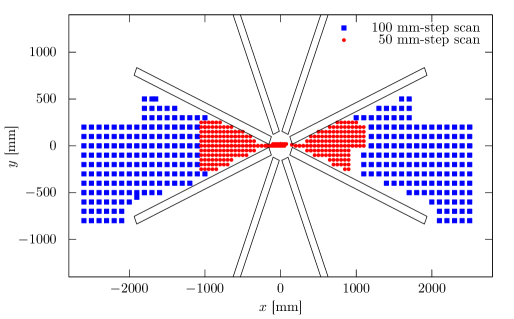
4.2.3 Surveying

During the set-up of the translation tables, the DESY Survey Group used a theodolite with a laser range-finder to measure the positions of survey targets on the I-beam to align the the tables with the axes of the OLYMPUS coordinate system. The Survey Group also measured the position of a target on a $z$-axis stepping motor over the course of a scan. The results indicated that the target did not follow a straight line, but in fact followed a trajectory which wiggled several millimeters up and down over the range in $z$. The shape of the trajectory was found to be repeatable, and so could be corrected, so long as the probe’s start and end position were known. We realized that we needed to survey the probe position at the start and end of each scan.

The DESY survey group provided a Leica Wild T3000 Total Station, and a Kern E2 Theodolite to allow OLYMPUS personnel to start and end positions in between measurement scans. Both devices can measure the polar and azimuthal angles to a point in space fixed by a telescope and cross-hairs. The total station can additionally measure the distance to a set of special reflective targets using a laser range-finder. We positioned the total station in the DORIS tunnel just downstream of OLYMPUS, while the theodolite was positioned on the opposite sector to have a face-on view of the probe at the start of each scan. A schematic of this positioning is shown in figure 4.4.

Figure 4.4: This schematic shows the orientation of the total station and theodolite relative to the magnet and measuring apparatus during measurements of the left sector, looking down on the experimental hall from above (not exactly to scale). The apparatus position is shown for the start of a scan. During a scan, the probe would be moved across the magnetic field region (from left to right in this image).

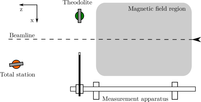
To use the laser-range finding feature of the total station, we needed to attach reflective targets to the measurement rod. The best system we could devise was to use cable ties to tightly fasten a loop in the target’s plastic backing around the rod. We aimed to keep the target cross hairs 50 mm from the probe position, which we checked by ruler. When using the longest rod, the target was sometimes blocked from view by one of the magnet’s supporting K-beams. For this rod, we attached a second reflective target and used the total station to calibrate its position relative to the first target.

This survey system depended on our knowing the positions of the theodolite and total station. We calibrated these positions daily using the survey targets that had already been fixed to the OLYMPUS support frame and the walls of the experimental hall. These positions of these targets had previously been ascertained by survey. By remeasuring them, the total station and theodolite positions could be fixed. Occasionally, the survey apparatus would get bumped out of carelessness, but it was easy to recalibrate the position by remeasuring the survey targets.

4.2.4 Procedure

During data taking, a crew of three people operated equipment to make measurements. One person controlled the translation tables from a computer station near the side wall, away from the fringe field of the magnet. A second person operated the theodolite to survey the probe tip start position. The third person used the total station to survey the reflective targets at each scan’s start and end position.

All of the scans for a given rod were performed at once, to minimize the number of times that a rod had to be exchanged. First, the medium rod measurements were taken (for the region 950 mm $<x<$ 1700 mm). Next, the short rod was installed for the region 1800 mm $<x<$ 2500 mm. Then the long rod was installed for the region 150 mm $<x<$ 900 mm. The brackets attaching the long rod were then adjusted to extend the long rod to cover the Møller region ($|x|<100$ mm). Finally, the vertical extension was added and the medium rod reattached to cover the area above the beamline, near the upper edge of the tracking volume. After these scans were completed on the left sector, the apparatus was taken apart and reassembled to measure the right sector.

A daily calibration procedure was designed and followed during data taking. Each morning, the theodolite and total station were each used to measure targets on the walls and frame to fix the theodolite and total station positions. The positions of the 1 m translation stands were checked with rulers against the positions specified by their electronic controllers. The zero-point on the Hall probe was reset using a Mu-metal cylinder. Finally, a test run was taken with the magnet turned off.

Changing Rods

A set of procedures was followed in order to change the rod. The work of mounting the probe in the rod, and attaching the rod with brackets to the translation tables was performed by a technician in the DESY group MEA 1. No easy way was found to align the probe in the rod, so the alignment was checked by using the theodolite, and then adjusted by hand. A reflective survey target was attached to the rod and positioned using a ruler. Finally, a survey scan was taken. The probe was moved and the target resurveyed at every step point in a scan. These data were used to correct for deviations in the probe position relative to its nominal position specified by the translation tables.

4.3 Analysis of the Survey Data

4.3.1 Determing the Probe Position

The first task for analyzing the magnetic field scans was the determination of the spatial position and orientation of the probe at each measurement point. The scanning procedure was designed to map out a grid in space, the translation tables deviated from their nominal positions by several millimeters, necessitating the survey procedure. The integration of the survey data was divided into three principal tasks:

• Determining the positions of the targets at the beginning and end of each scan

• Determining the probe positions relative to these targets

• Modeling the trajectory of the probe along the length of the scans.

Each of these topics is covered in the following sections.

Determining Target Positions

For each scan, the scanning rod was surveyed using total station and theodolite. The two devices are similar; they both have a telescope with crosshairs and can report the polar and azimuthal angles of the crosshairs. The total station can also measure the distance to a reflective target using a laser. This additional distance measurement, combined with the measurement of the two angles, uniquely constrains the target point in three dimensional space, making the total station far more useful than the theodolite. Though the theodolite was extremely useful for making sure that the probe was aligned during the installation of each new rod, we never ended up using its survey data, and for the remainder of this chapter, when I mention survey data, I’ll be referring only to that of the total station.

The first task in analyzing the survey data was calibrating the total station’s position and orientation. This was determined from the daily calibration measurements of targets around the hall and on the OLYMPUS frame. This gave us a way to translate the total stations measurements into three dimensional positions in the OLYMPUS coordinate system. We found that the total station position varied only slightly day to day, with the exception of a few large displacements, which we attribute to times when the total station was moved by accident.

The start and end positions of each scan were then mapped into OLYMPUS coordinates. On examination of this data, it was found that a handful of points had anomalous positions due to transcription errors. The total station measurements were recorded by pen and paper, and if digits were transposed or mis-written, this, thankfully, produced a noticable abberation in position. We endeavored to correct as many of the transcription errors as we could find, approximately a few dozen over 700 scans. To search for these errors, the position data were plotted in several ways to look for inconsistencies. One way was to plot the difference between the target position and the nominal scan position. If the position data were correct, then they would appear in this plot to be clustered around a constant value: the difference between the target position and the probe position. Positions that were very far from the cluster, were likely to have transcription errors. Another useful plot was the difference between the start and end positions of a scan. In the $x$ and $y$ directions, this difference clustered around zero. Outliers were likely to have errors. After examining every measurement, all of the positions were well-clustered to within a few millimeters or better, as can be seen in figure 4.5.

Figure 4.5: The start and end positions were not exactly at the nominal scan position due, demonstrating how valuable having a survey was. The positions are all well-clustered, indicating that we have fixed all of the (major) transcription errors.

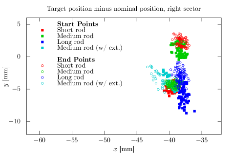
One observation that was made during this process was that during the left sector measurements, the $Z$ axis of the translation table came out of alignment with the OLYMPUS $Z$ axis. This occurred between the measurement of the end point of scan 93 and the start point of scan 94. Between these scans, the large $XY$ tables were adjusted, so it is possible that during this movement, the tables made contact with part of the magnet. This misalignment posed no problems because the survey data allowed the probe positions for scans after 94 to be corrected.

Determining the Probe Positions

The next task was to determine the position of the Hall probe relative to the positions of the total station targets. The reflective targets were fixed to the measurement rods by hand using cable ties, but their positions were not precisely known. A set of offsets was needed to establish the position of the Hall probe relative to the positions of the targets on each rod.

Reflective targets were fixed to the rod using cable ties, and positioned 50 mm from the probe using a ruler. We attempted to use the total station to check the angles between the probe and target but could not fix the probe position in the cross hairs since we were looking side-on. Therefore we assumed that the probe was always 50 mm away from the target in $x$, and 0 mm in $y$. The deviation $z$ was directly related to the thickness of each rod, which we checked using a micrometer with calipers.

For some scans the target close to the probe was not visible, and a second target further up the rod was needed. We used the total station to fix the distance between the two targets in three dimensions when both targets were visible. This allowed us to produce an offset for use when the near target was not visible.

Scan Trajectories

Early on, during the set up of the measurement apparatus, it was noticed that the translation tables did not maintain a consistent vertical position over the course of the full range in the $Z$ direction. Instead, the table height fluctuated several millimeters over the course of a scan. Corrections to the scan positions were required to accurately reflect the true trajectory of the Hall probe over the course of a scan.

To measure these trajectories, a test scan was made for each rod, in which the rod was stepped in increments of $Z$ and the target positions were measured with the total station. From these measurements, it was found that the overall shape of these fluctuations was consistent for each set-up of the apparatus, i.e., all scans on the left sector had similarly shaped trajectories, but these were different from the shape of the trajectories on the right sector. It was also found that the magnitude of these fluctuations depended predictably on the length of the rod being used. In fact it was sufficient to parameterize the trajectories of the Hall probe in the following way:

$$x_{r,s}(z)=x_{s}(z)+L_{r}\cos\left(\theta_{s}(z)\right)+\text{linear term},$$ (4.1)

$$y_{r,s}(z)=y_{s}(z)+L_{r}\sin\left(\theta_{s}(z)\right)+\text{linear term}.$$ (4.2)

Index r represents the rod being used, while index s represents the sector (left or right). The trajectory could be expressed in terms of three functions $x_{s}(z)$, $y_{s}(z)$, and $\theta_{s}(z)$ that were consistent across each sector, as well as the rod length $L_{r}$ which was measured. The three functions were extracted using a fit to the calibration data, and the residuals were found to be sufficiently small. A linear term was used to match the trajectory to each scan’s start and end points. Fits to trajectories on the left sector from three rods are shown in figure 4.6.

Figure 4.6: The deviations in scan position could be corrected using calibration data fit with a simple parameterization.

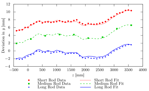
Results

Figure 4.7: This figure shows our measurement of the magnetic field in the $y$ direction along the $y=0$ plane.

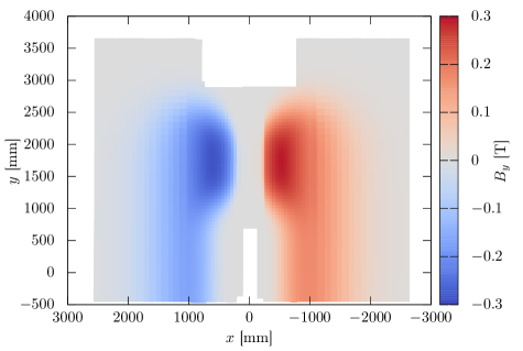
By determining the start and end points of each scan, mapping the probe position to the target position, and correcting the trajectories between endpoints, we have mapped the magnetic field data into OLYMPUS coordinates. The field in the $y=0$ plane, which is nominally the center of the tracking acceptance, is shown in figure 4.7. We can see that the field points downwards in the left sector ($x>0$) and upwards in the right sector ($x<0$).

4.3.2 Generating a Field Map

Overview

The result of the work in section 4.3.1 was to convert the magnet field measurements into a list of positions and corresponding field vectors. The challenge of this section is to turn that data into a field map; a value of the magnetic field as a function of position. This requires determining the magnetic field between nearby measurement points (interpolation) and at points that are outside the spatial extent of the measurements (extrapolation). Interpolation in three dimensions is straight-forward if the measurement points fall on a regular grid. Because of the position deviations of our apparatus, our data do not. Direct interpolation on an irregular grid is a much more difficult proposition and is one that we sought to avoid.

Instead, we chose to build a model of the magnetic field, parameterized by the positions and orientations of the magnet coils, and to fit these parameters to our measured data. This approach carried two advantages. The first was that after fitting, we could then use the model to calculate the field at any arbitrary point in space. The second was that any errant data points, for which we assigned an incorrect position or recorded the wrong field, would have their influence in the fit dampened by all of the other measurements. The challenge of this approach was to create a model that could both accurately reproduce the measured data, while also being well constrained by it. We settled on a 35-parameter model, in which the parameters represented position offsets, rotation offsets, and scaling parameters.

Magnet Model

We chose to model the OLYMPUS magnet with a collection of line segment-shaped currents that traced the position of the current-carrying copper bars within each coil. In reality, current is carried through the volume of each copper bar, but by approximating the bars by filaments, we avoided having to model the current distribution over the cross-sectional extent of each bar. The field produced by a line-segment of current is also easy to calculate. By integrating the Biot-Savart Law, we find that for a segment centered at point $\vec{c}$, carrying current $I$, and with a length vector $\vec{L}$, the field at position $\vec{p}$ is given by:

$$\vec{B}=\frac{\mu_{0}I}{4\pi\beta^{2}}\left[\frac{\left(\alpha+|\vec{L}|/2\right)}{\left|\vec{c}-\vec{p}+\vec{L}/2\right|}-\frac{\left(\alpha-|\vec{L}|/2\right)}{\left|\vec{c}-\vec{p}-\vec{L}/2\right|}\right]\cdot\left(\vec{c}-\vec{p}\right)\times\vec{L},$$ (4.3)

$$\alpha\equiv\hat{L}\cdot\left(\vec{c}-\vec{p}\right),$$ (4.4)

$$\beta^{2}\equiv\left(\vec{c}-\vec{p}\right)^{2}-\alpha^{2}.$$ (4.5)

The nominal OLYMPUS coil shape is irregular, but can be broken down into straight segments and circular arc segments. The straight segments were trivially represented by filaments. Rather than calculating the field produced by arcs, which requires special functions called Appell functions, we chose to approximate the arc-shaped segments with collections of line-segments. The proper placement of these line segments is a non-trivial exercise. If the start and end points lie on the path of the arc, then the area of the arc is diminished and the dipole moment decreased. The segments can be spread out to preserve the area of the arc, but this means that the end points first and last segment will no longer lie on the end points of the arc. If the arc is a portion of a current loop, then the loop will not be continuous at the start and end points of the arc. To balance these concerns, it was decided to position the segments so that the first and last segment began and ended, respectively, on the endpoints of the arc, preserving continuity of any current loops. The other segments’ endpoints would be expanded outward to a larger radius $R^{\prime}$ to maintain the area of the arc. The expression for $R^{\prime}$, derived from geometry, is

$$R^{\prime}=R\left(\sqrt{\frac{1}{(N-2)^{2}}+\frac{\theta_{a}}{(N-2)\sin(\theta_{a}/N)}}-\frac{1}{N-2}\right),$$ (4.6)

where N is the number of segments used to approximate the arc, and $\theta_{a}$ is the angle subtended by the arc.

In our model, each coil was identical in shape and composition. Each coil was represented by 26 current loops, arranged in two rows of 13, in the nominal positions of the copper bars within the coils. The two $180^{\circ}$ arcs of each loop were approximated by 180 line segments, while the two $38.58^{\circ}$ arcs were approximated by 40 segments.

Fitting the Magnetic Field Data

To fit our model, we had to choose a set of free parameters to vary. When we began, all we knew were the nominal positions of each coil. We did not know what freedom needed to be introduced to the model to accurately describe our magnetic field data. Did the coil positions need to vary only in radius from the beamline, or in orientation as well? Was the toroid axis where we thought it was? Were the coils the correct size?

Our approach was to try many different combinations of free parameters and then to simultaneously monitor the fit residuals and the parameter values themselves. Our fitting criterion was that we minimize the sum of the squared residuals: $\sum|\vec{B}_{\text{meas.}}-\vec{B}_{\text{model}}|^{2}$. Fits that converged on minima where the parameters were wildly different than their expected values indicated that some parameters in our model were not well-constrained by the data, and should not be given freedom. If adding a free parameter reduced fit residuals without causing any parameters to go wild, we took that as a sign that more freedom could be added.

One natural parameter set consisted of the three positions and three rotations for all eight coils. However the final positions for the top two and bottom two coils were wildly different than what one would expect. We have no measurements close to those coils, and so they had no firm constraints on their positions and rotations. Instead, it was more productive to give the four coils surrounding the tracking volume (numbered 0, 3, 4, and 7) more freedom, while restricting the top and bottom pairs of coils (numbered 1, 2, 5, and 6).

We settled on a parameter set with 35 free parameters. The four coils adjacent to the tracking volume were given 24 parameters to fully describe their positions and orientations. The remaining four coils were collectively given eight: three positions to specify the toroid origin, three rotations to specify the toroid axis, one to specify the distance of the coils from the axis, and, lastly, one parameter to describe the amount of rotation in the plane of the coil. Of the remaining three parameters, two were scaling factors in the plane of the coils, allowing all eight coils to collectively shrink or expand in two dimensions. The final parameter was the current in the magnet, which the fit predicted to within 0.2%. The values of these parameters, after the fit converged, are shown in table 4.1. For reference, if the magnet occupied its nominal position, the parameters would have all been 0, with the exception of the scaling factors $S_{x}$ and $S_{y}$, which would be 1, and the current, which would be 5000 A.

Par.	Value	Par.	Value	Par.	Value	Par.	Value
$\Delta\rho_{0}$	26.58 mm	$\Delta\rho_{3}$	24.64 mm	$\Delta\rho_{4}$	-4.962 mm	$\Delta\rho_{7}$	-1.494 mm
$\Delta\phi_{0}$	0.01∘	$\Delta\phi_{3}$	-0.006∘	$\Delta\phi_{4}$	-0.006∘	$\Delta\phi_{7}$	0.002∘
$\Delta z_{0}$	8.214 mm	$\Delta z_{3}$	1.429 mm	$\Delta z_{4}$	0.332 mm	$\Delta z_{7}$	22.74 mm
$\Delta\theta_{x0}$	-0.040∘	$\Delta\theta_{x3}$	-0.065∘	$\Delta\theta_{x4}$	0.12∘	$\Delta\theta_{x7}$	0.547∘
$\Delta\theta_{y0}$	-0.939∘	$\Delta\theta_{y3}$	1.141∘	$\Delta\theta_{y4}$	1.1∘	$\Delta\theta_{y7}$	-0.891∘
$\Delta\theta_{z0}$	0.402∘	$\Delta\theta_{z3}$	0.635∘	$\Delta\theta_{z4}$	-0.846∘	$\Delta\theta_{z7}$	-0.492∘
$x$	3.357 mm	$\alpha_{x}$	1.368∘	$S_{x}$	0.986	$\theta_{\text{coil}}$	-0.05∘
$y$	-21.7 mm	$\alpha_{y}$	0.017∘	$S_{y}$	0.998	$\Delta\rho$	12.35 mm
$z$	4.633 mm	$\alpha_{z}$	-0.163∘	$I$	5007 A

Table 4.1: The final fit had 35 free parameters. Coils 0, 3, 4, and 7 were given full freedom because they surrounded the tracking volume and were well constrained by the measurements.

Results

Figure 4.8: The magnetic field map is shown in the $y=0$ plane.

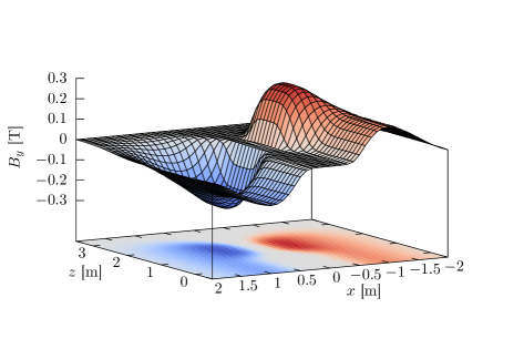
Figure 4.8 shows the magnetic field in the $y$ direction, as calculated from the field model after fitting the parameters to data. Qualitatively, there are no significant changes to the shape of the field compared with our expectations. More can be learned from looking at the residuals of the fit, shown for the $y$ direction in figure 4.9.

Figure 4.9: The nominal field was not too far off from reality, but with slight adjustments in the positions of the coils, the fitted model did a better job of matching the field measurements.

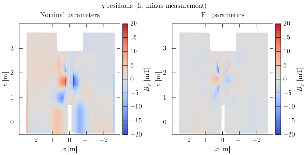
The fit improved the model’s match to our measurements from an r.m.s. residual $\sqrt{\frac{1}{3N}\sum|\vec{B}_{\text{meas.}}-\vec{B}_{\text{model}}|^{2}}$ (where $N$ is the number of measurement points) from 3.198 mT to 1.873 mT. These residuals do not represent random Gaussian errors, as can be seen in figure 4.9. There are specific regions that are not modelled well. This can be caused both by inadequacy of the model and by errors in the survey. As examples, in the first case, perhaps the coil arcs are not exactly circular or the conducting bars are unevenly spaced. In the second case, we may have assigned the wrong positions to measurement points because of mis-measuring the probe to reflective target distance. In the first case, the model is to blame. In the second case the model helps by constraining what would otherwise be inaccurate measurements.

4.4 Using the Field Map in Software

4.4.1 Spline Interpolation

To calculate the magnetic field at a given position, the magnetic field model of the previous section works by applying equation 4.3 to each current segment in the ensemble that makes up all eight coils. This method is fast enough for some applications (such as fitting free parameters, or examining the shape of the field), but is far too slow to be used for simulation of tracks or for track reconstruction. Both of these applications require hundreds if not thousands of field queries per track, and the rates need to scale in order to track the billions of events in the OLYMPUS data set. A significant speed up was needed.

Our solution was to use the magnetic field model to pre-compute field vectors (and derivatives, via finite differences) on a grid over the spectrometer volume. A fast field calculation could be performed by using three dimensional spline interpolation between the nearest grid points. Spline interpolation was preferred to linear interpolation so that the first derivatives of the field would be continuous and non-zero, helping the simulation software query the field appropriately.

Interpolation would have been possible directly on the measurement data. There were three reasons for not pursuing this approach. Primarily, the measurement data only covered a limited amount of space, and extrapolation was needed as well as interpolation. However in addition to this, the algorithms for interpolation on a non-uniform grid are much slower than those on a uniform grid. Lastly, the presence of a fitting step in between the measurements and interpolation served to smooth the data and remove errors that might be associated with faulty survey measurements.

The grid was chosen to range from -2.5 m to 2.5 m in $x$, from -1 m to 1 m in $y$, and from -0.5 m to 3.5 m in $z$ with 50 mm spacing. The grid had a total of 418,241 points. The choice of grid had to balance point density, which would reduce the errors from interpolation with the size of the grid, which the simulation software would need to store in memory.

The interpolation scheme was based on an algorithm by Lekien and Marsden [86] that uses eight values per field direction $i$, per grid point $P$:

$$C_{i,P}=\left\{B_{i},\frac{\partial B_{i}}{\partial x},\frac{\partial B_{i}}{\partial y},\frac{\partial^{2}B_{i}}{\partial x\partial y},\frac{\partial B_{i}}{\partial z},\frac{\partial^{2}B_{i}}{\partial x\partial z},\frac{\partial^{2}B_{i}}{\partial y\partial z},\frac{\partial^{3}B_{i}}{\partial x\partial y\partial z}\right\}.$$

My colleague Brian Henderson developed several improvements to the algorithm [82]. The first was to refactor the spline basis functions to reduce the memory needs, or alternatively reduce the number of multiplications needed per query. To see how this works, consider that a spline can be written in a basis such that:

$$B_{i}(x,y,z)=\sum_{l,m,n=0}^{3}a_{i,lmn}x_{f}^{l}y_{f}^{m}z_{f}^{n}\>\>\>\>i\in\left\{x,y,z\right\},$$ (4.7)

where the coefficients $a_{i,lmn}$ are polynomial functions of the field and derivatives at the eight surrounding grid points. The calculation of $a_{i,lmn}$ requires three $64\times 64$ matrix multiplications, which can either be computed on the fly, or precomputed and stored. The first option is slower; the second option requires significant memory, which scales with the volume of the grid. Brian refactored the splines into basis functions:

$$f_{0}(x)= (x-1)^{2}(2x+1)$$ (4.8)

$$f_{1}(x)= x(x-1)^{2}$$ (4.9)

$$f_{2}(x)= x^{2}(3-2x)$$ (4.10)

$$f_{3}(x)= x(x-1),$$ (4.11)

so that the spline could be written in the form:

$$B_{i}(x,y,z)=\sum_{l,m,n=0}^{3}b_{i,lmn}f_{l}(x)f_{m}(y)f_{n}(z)a_{i,lmn}\>\>\>\>i\in\left\{x,y,z\right\},$$ (4.12)

where the coefficients $b_{i,lmn}$ are the values $C_{i,P}$ for the eight surrounding grid points. If we denote these eight points as a vector $P_{j}$:

$$P_{j}=\{xyz,Xyz,xYz,XYz,xyZ,XyZ,xYZ,XYZ\},$$

where miniscule denotes a grid point with a smaller value of the coordinate than the queried point, and majiscule denotes a grid point with a larger value of the coordinate than the queried point, then

$$b_{i,lmn}= C^{k}_{i,P_{j}},$$ (4.13)

$$j= 4\left(\frac{n}{2}\%2\right)+2\left(\frac{m}{2}\%2\right)+\left(\frac{l}{2}\%2\right),$$ (4.14)

$$k= 4(n\%2)+2(m\%2)+(l\%).$$ (4.15)

The memory costs of precomputation are eliminated, and the matrix multiplications are avoided.

The second improvement was to store the values $C_{i,P}$ in an array in memory so that the coefficients for each of the eight grid boxes were grouped into sets of continuous blocks of memory. This permitted Single-Instruction Multiple Data (SIMD) computing, which could improve the speed of queries for some computer architectures.

4.4.2 Field in the Beamline Region

Figure 4.10: The magnet model did not do a good job in the beamline region, as seen here for the $x$ component of the field.

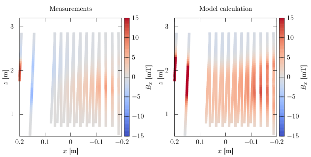
The field model was unable to reproduce features in the magnetic field in the beamline region. This can be seen in figure 4.10. This was a difficult region to model correctly because it is physically close to the edges of all eight coils, and any changes in position in any coil can introduce gradients in the beamline region. It is also a region where not many measurements were made. It was difficult to stick the probe in between the coils, and measurements could only be taken from the left or right, not from above or below. Still, the measurements indicated some clear features that the model could not reproduce, which provoked concern for the simulation of Møller/Bhabha events which pass through the beamline region. We decided that simulations in this region (defined by $|x|<100$ mm, $|y|<50$ mm, and $500<z<3000$ mm) would use a different interpolation scheme.

Figure 4.11: The 2011 measurements of the beamline region (shown in circles) match all the features from the main 2013 measurements (shown as bands).

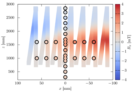
Our first cross check was the data from field measurements taken in 2011 of the field in the beamline region. These measurements were used to align the coils, since the beamline field is zero if the toroid is perfectly aligned. These measurements were made with a completely different apparatus and survey technique. The results, shown in figure 4.11, confirmed that the features we measured in 2013 are correct, and not the result of spurious measurements.

We decided to interpolate directly on the beamline field measurements. Since the measurements were all made at $y=0$, we made the approximation that the field did not vary in $y$. This allowed us to use a two-dimensional Lagrange polynomial interpolation over $x$ and $z$ [87].

In the region inside the target chamber (defined by $|x|<100$ mm, $|y|<50$ mm, and $|z|<500$ mm), we had no 2013 measurements, since the chamber was still in place and obstructed the probe. But we did have 2011 measurements, which became a lot more trustworthy when we showed that they matched the 2013 measurements in the beamline region. The 2011 measurements in the target chamber region were taken along the $x=0,y=0$ line. We assumed that, in this region, there was no variation in $x$ or $y$, and we modelled the $z$ variation by fitting a quadratic function to each component from the 2011 measurements.

4.4.3 Field Near the Coils

Our spline interpolation procedure ran into trouble around grid points that were very close to any of the line-segments of current in the model. One effect of modeling the conductors as line segments is that the field diverges at the segments. The field and derivatives get very large close to the segments. Ordinarily, tracks never get that close to the magnet coils. The coils are positioned at $\phi=\pm 22.5^{\circ}$, while the tracking acceptance covers the region $|\phi|<15^{\circ}$. However, when interpolating on a grid, some of the grid points will inevitably be close to segments, and any grid point with enormous derivatives will spoil the interpolation over any of the boxes with which it is associated. The worst areas were a few hundred millimeters from the beamline where the tracking acceptance passes closest to the inner edges of the coils.

Our solution was to recalculate the field and derivatives for grid points with $|\phi|>15^{\circ}$ using a different technique, making use of the approximate azimuthal symmetry of the toroid. For such a grid point, we would first calculate the magnetic field and derivatives at a point with the radius from the beamline, and same $z$, but for $\phi$ equal to the nearest $\pm 15^{\circ}$ plane. We would set all azimuthal derivatives to zero (assuming perfect azimuthal symmetry), and then rotate the vectors back to the original grid point. For example, if a grid box were to fall at $r=1$ m, $z=2$ m, and $\phi=20^{\circ}$, we would first calculate the field and derivatives $\{\frac{\partial\vec{B}}{\partial r},\frac{\partial\vec{B}}{\partial z},\frac{\partial^{2}\vec{B}}{\partial r\partial z}\}$ at the point where $r=1$ m, $z=2$ m, and $\phi=15^{\circ}$, assuming all other derivatives were 0. We would then rotate all the vectors by $5^{\circ}$ so as to properly correspond to the position where $\phi=20^{\circ}$.

We used spline interpolation on this new grid exactly as before. We found that the simulated trajectories at $\phi=\pm 15^{\circ}$ were essentially the same as those simulated with the non-interpolated (and very slow) Biot-Savart field model.

4.5 Improvements for Future Field Measurements

Though the OLYMPUS magnetic field measurements turned out successfully, if I were involved in a similar project in the future, there a few things I would do differently. I share these ideas in case they can help the reader save time and work on any future field measurements.

4.5.1 Reliability of the Translation Tables

The largest fraction of total effort went into surveying and interpreting survey data. This could have been avoided if we have used translation tables that could deliver the desired accuracy. The problem, as far as we can tell, was that the long 4 m table rested on an I-beam which was slightly deformed, giving the entire table a degree of deformation. Because of the table position and probe position now deviated by several millimeters, we had to introduce a survey procedure. Having a theodolite operator and total station operator effectively tripled the man-hours needed for the magnetic field measurements. And furthermore a great deal of analysis time was sunk into making sense out of the survey data. I now appreciate that work done ahead of time to test the accuracy of the translation tables would have been recovered many times over if we had avoided this pitfall.

4.5.2 Uniform vs. Non-Uniform Measurement Spacing

Since the translation tables had deviations, our measurements were no longer in a regular grid. Interpolation on regular grids is simple, while interpolation on irregular grids is an ordeal. If our tables had delivered uniformly spaced measurements, direct interpolation would have been an option for us.

If uniformly-spaced measurements aren’t feasible, then it makes no difference if the measurements are spaced nearly evenly or completely randomly. It struck us that a Hall probe mounted to a small helicopter drone, combined with a automatic laser tracker could have given us about the same performance as our immense translation table apparatus. A drone could fly randomly back and forth through the magnet, and as long as the laser tracker could record the position at each measurement point, it would be quick work to survey the magnetic field.

4.5.3 Better Survey Marks

It felt a little bit silly to use a high-precision laser range-finding total station to measure reflective targets that were positioned using a ruler. There is a always weakest link, and in our survey, it was the calibration of the probe to target distance. Had we not been under time pressure to complete the measurements, I think we could have devised a modification to the carbon fiber rods that would have fixed the survey target in relation to the probe. At the very least we might have been able to check the distance with a micrometer and calipers instead of a ruler.

Chapter 5 Radiative Corrections

5.1 Introduction

“Radiative corrections” is the general moniker for the procedure of accounting for higher order terms in a perturbative expansion. Often, radiative corrections depend on the properties of an experiment’s apparatus, e.g., the resolution, acceptance, or threshold of a detector. In these cases, it is crucial for the experimenters to apply radiative corrections to their data because, without them, the results of the experiment cannot be interpreted.

Figure 5.1: There is a single leading order diagram: one-photon exchange.

As an example, let’s consider radiative corrections for the case of an unpolarized elastic electron-proton cross section measurement. The leading order diagram is the one-photon exchange diagram, shown in figure 5.1. By attributing the entire cross section to one-photon exchange, one can extract the form factors $G_{E}$ and $G_{M}$ that describe the proton vertex. Let’s imagine that this example experiment is an inclusive measurement, that is, we will position a spectrometer at scattering angle $\theta$ to detect the electron and the proton will go undetected. The electron spectrometer will tell us the momentum of the detected electron. To measure the cross section, we will count the number of electrons detected by our spectrometer with the proper elastic momentum, and divide by the integrated luminosity. We will disregard electrons with lower momenta because they are the result of inelastic processes (and of course, it is not kinematically possible for electrons to emerge with greater than the elastic momentum). The energy spectrum from the spectrometer might look like the top plot in figure 5.2.

Figure 5.2: This figure shows how radiative effects complicate the analysis of an inclusive elastic electron scattering experiment. Both plots show sketches of what momentum spectra might look like in a spectrometer positioned at fixed scattering angle. The top plot represents an idealized case, where radiative effects do not exist; it is simple to separate elastic events from background with a simple cut on momentum. The bottom plot represents a more realistic case, where the elastic peak has a long radiative tail. The choice of cut position can greatly change how many elastic events are recorded. Radiative corrections, which model the shape of the tail, are needed to remove the dependence on cut position.

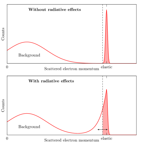
This approach is complicated by the emission of soft bremsstrahlung photons. These photons, which go undetected, remove a small amount of energy from the scattered lepton. Instead of seeing a narrow peak in our momentum spectrum at the elastic momentum, we will see a long tail in the distribution towards lower momenta, sketched in the bottom plot of figure 5.2. When we analyze our data, we must make a distinction between elastic and inelastic electrons, but where we make this distinction clearly affects our result. If we require more stringent limits on electron momentum, our extracted cross section will be smaller. If we consider more of the tail to be elastic, then our extracted cross section will be larger. The result is meaningless, because it can be tuned.

Figure 5.3: There are four $\mathcal{O}(e^{3})$ bremsstrahlung (inelastic) diagrams.

Figure 5.4: There are several $\mathcal{O}(e^{3})$ elastic diagrams, many of which have divergences.

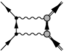
Instead, we must model the shape of the “radiative tail” so that we can recover the one-photon exchange cross section as a function of how we define our acceptance for elastic events. To do this, we should calculate the bremsstrahlung diagrams, shown in figure 5.3, and integrate them over some window of electron momentum acceptance. This approach would work, except for the fact that this integral diverges. The divergence is cancelled by other divergences in the $\mathcal{O}(e^{3})$ corrections to elastic scattering, shown in figure 5.4. To account for soft bremsstrahlung, one must account for these other diagrams as well. After doing this, one arrives at a correction factor for recovering the one-photon exchange cross section:

$$\frac{d\sigma}{d\Omega}_{1\gamma}(\theta)=\frac{d\sigma}{d\Omega}_{\text{meas.}}(\theta,\Delta p)/(1+\delta(\theta,\Delta p)).$$ (5.1)

In this chapter, I will first discuss the previous radiative corrections procedures for elastic electron-proton scattering. I will then discuss the specific radiative correction needs for OLYMPUS, including the details of the OLYMPUS radiative event generator that I, along with Rebecca Russell and Jan Bernauer, developed for OLYMPUS simulations. I will conclude with some discussion about the differences in the various correction models that the generator can simulate.

5.2 Radiative Corrections to Elastic $ep$ Scattering

5.2.1 Diagrams

The matrix element for elastic $ep$ scattering, $\mathcal{M}_{e}p$, can be expanded into a Feynman series in powers of the fine structure constant $\alpha$:

$$\mathcal{M}_{ep}=\alpha\mathcal{M}_{1}+\alpha^{2}\mathcal{M}_{2}+\alpha^{3}\mathcal{M}_{3}+\ldots\quad.$$ (5.2)

The cross section, which depends on the square of the matrix element, can be similarly expanded:

$$\sigma_{ep}\propto|\mathcal{M}_{ep}|^{2}=\alpha^{2}|\mathcal{M}_{1}|^{2}+2\alpha^{3}\text{Re}\left[\mathcal{M}_{1}\mathcal{M}_{2}\right]+\ldots\quad.$$ (5.3)

The measured cross section will also have a contribution from bremsstrahlung, which goes as $\alpha^{3}$ at leading order. The bremsstrahlung diagrams are inelastic, so the contribution to the elastic cross section will be limited to the region in which the photon energy is small and the kinematics are “nearly elastic:”

$$\sigma_{\text{meas.}}\propto\alpha^{2}|\mathcal{M}_{1}|^{2}+2\alpha^{3}\left\{\text{Re}\left[\mathcal{M}_{1}\mathcal{M}_{2}\right]+\int_{\text{small~{}}E_{\gamma}}d\vec{k}_{\gamma}|\mathcal{M}_{\text{brems.}}|^{2}\right\}\ldots\quad.$$ (5.4)

Let’s consider which specific diagrams contribute to the different terms. In the leading term, $|\mathcal{M}_{1}|^{2}$ is the square one-photon exchange term. At the order of $\alpha^{3}$, there are two groups of terms that contribute. There are the $\mathcal{M}_{1}$ and $\mathcal{M}_{2}$ interference term, Re$[\mathcal{M}_{1}\mathcal{M}_{2}]$, and the bremsstrahlung term. The bremsstrahlung can be broken up into groups based on the dependence on the lepton charge $z$:

• Lepton bremsstrahlung ($z^{4}$): $\left|\parbox[h][56.9055pt][c]{56.9055pt}{\includegraphics[width=56.9055pt]{brems_ei.pdf}}+\parbox[h][56.9055pt][c]{56.9055pt}{\includegraphics[width=56.9055pt]{brems_ef.pdf}}\right|^{2}$

• Lepton-proton bremsstrahlung interference ($z^{3}$):
  $\left(\parbox[h][56.9055pt][c]{56.9055pt}{\includegraphics[width=56.9055pt]{brems_ei.pdf}}+\parbox[h][56.9055pt][c]{56.9055pt}{\includegraphics[width=56.9055pt]{brems_ef.pdf}}\right)^{\dagger}\left(\parbox[h][56.9055pt][c]{56.9055pt}{\includegraphics[width=56.9055pt]{brems_pi.pdf}}+\parbox[h][56.9055pt][c]{56.9055pt}{\includegraphics[width=56.9055pt]{brems_pf.pdf}}\right)$

• Proton bremsstrahlung ($z^{2}$): $\left|\parbox[h][56.9055pt][c]{56.9055pt}{\includegraphics[width=56.9055pt]{brems_pi.pdf}}+\parbox[h][56.9055pt][c]{56.9055pt}{\includegraphics[width=56.9055pt]{brems_pf.pdf}}\right|^{2}$

All three of these groups diverge when integrated down to zero photon energy. These divergences cancel against similar divergences in Re$[\mathcal{M}_{1}\mathcal{M}_{2}]$. The lepton bremsstrahlung divergence, proportional to $z^{4}$, cancels against a divergence in:

$$2\text{Re}\left[\parbox[h][56.9055pt][c]{56.9055pt}{\includegraphics[width=56.9055pt]{ope.pdf}}^{\dagger}\parbox[h][56.9055pt][c]{56.9055pt}{\includegraphics[width=56.9055pt]{ver_cor_e.pdf}}\right],$$

the lepton vertex correction. The proton bremsstrahlung divergence, proportional to $z^{2}$, cancels against a divergence in:

$$2\text{Re}\left[\parbox[h][56.9055pt][c]{56.9055pt}{\includegraphics[width=56.9055pt]{ope.pdf}}^{\dagger}\parbox[h][56.9055pt][c]{56.9055pt}{\includegraphics[width=56.9055pt]{ver_cor_p.pdf}}\right],$$

the proton vertex correction. The divergence in lepton-proton bremsstrahlung interference cancels against a divergence in:

$$2\text{Re}\left[\parbox[h][56.9055pt][c]{56.9055pt}{\includegraphics[width=56.9055pt]{ope.pdf}}^{\dagger}\left(\parbox[h][56.9055pt][c]{56.9055pt}{\includegraphics[width=56.9055pt]{tpe_box.pdf}}+\parbox[h][56.9055pt][c]{56.9055pt}{\includegraphics[width=56.9055pt]{tpe_cross.pdf}}\right)\right],$$

the interference between one- and two-photon exchange. The only other term that contributes at order $\alpha^{3}$ is vacuum polarization:

$$2\text{Re}\left[\parbox[h][56.9055pt][c]{56.9055pt}{\includegraphics[width=56.9055pt]{ope.pdf}}^{\dagger}\parbox[h][56.9055pt][c]{56.9055pt}{\includegraphics[width=56.9055pt]{vac_pol.pdf}}\right],$$

which does not contain a problematic divergence.

5.2.2 Soft vs. Hard Two-Photon Exchange

Two-photon exchange must be included in radiative corrections in order to cancel the divergence in lepton-proton bremsstrahlung interference. However, as mentioned in chapter 2, it cannot be calculated in a model-independent way. However, it can be calculated exactly in the limit in which one of the photons carries no momentum, i.e., is soft. It is precisely this soft two-photon exchange which has the divergence necessary to cancel that of bremstrahlung interference. The standard radiative corrections schemes (which will be outlined in the following section) have proceeded by making an arbitrary distinction between soft two-photon exchange and hard two-photon exchange. The soft two-photon exchange is calculated and included. The hard two-photon exchange is neglected.

The distinction between hard and soft two-photon exchange is completely arbitrary. Not all radiative corrections schemes employ the same distinction. A measurement must report which radiative correction scheme (and thus which soft definition) was used in order for the result to be interpretable.

Previous cross section measurements—the ones that see a form factor discrepancy—have all used this radiative correction schemes employing this hard-soft distinction approach. The form factor discrepancy exists despite accounting for soft two-photon exchange. OLYMPUS aims to measure the contribution from hard two-photon exchange, which is the remaining piece that has been typically neglected.

5.2.3 Previous Work on $ep$ Radiative Corrections

Schemes for radiative corrections for electron scattering have been devised as early as the 1940s [88], and have generally proceeded in the same fashion as my example from the introduction. The goal is to recover the one-photon exchange cross section because form factors are defined in the one-photon exchange frame work. All of the earliest radiative correction schemes assume an inclusive experiment, in which only the electron is detected, and that energy/momentum of the electron is measured by the detector (and in the limit $m_{e}\rightarrow 0$, the energy and momentum are the same). These schemes assume that the experimenter will define an energy window of width $\Delta E$, such that electrons with energies between the elastic energy $E_{el.}\equiv Em_{p}/(m_{p}+2E\sin^{2}\frac{\theta}{2})$ and $E_{el.}-\Delta E$ will count towards the cross section. These schemes prescribe a correction $\delta$ such that:

$$d\sigma_{meas.}=d\sigma_{1\gamma}\times(1+\delta(\theta,\Delta E)).$$ (5.5)

The experimenter chooses an appropriate $\Delta E$ given the resolution limits of the detector, corrects the data, and recovers the one-photon exchange cross section.

The landmark radiative corrections procedure is that of Mo and Tsai [89] (1969), which built on the earlier work of Tsai [90] (1961). Meister and Yennie also produced a work based on Tsai, but with some approximations to make the the formula easier to calculate with computers of that era [91]. Though Mo and Tsai’s work is considered standard, there have been more recent attempts to update it. In 2000, Maximon and Tjon produced a calculation [92] that used fewer approximations, employed a different definition of soft two-photon exchange, and included a dipole model of the proton’s form factors in order to add proton structure information to the proton vertex correction. A comparison of these three corrections is shown in figure 5.5.

Figure 5.5: Standard radiative corrections are shown for 2 GeV electron beam, and a scattering angle of $60^{\circ}$. The different corrections make slightly different assumptions but make the same qualitative predictions: $\delta$ is negative, small, and monotonically increasing as function of $\Delta E$.

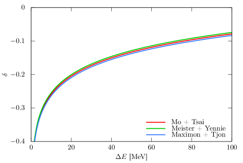
In 2001, Ent et al. published a radiative corrections procedure [93] used in the NE18 experiment that reworks Mo and Tsai’s equations to produce a $\delta$ that depends on the missing energy $W$, instead of electron energy loss $\Delta E$, because $W$ is a more relevant quantity in coincidence experiments. The paper goes on to explain methods for applying radiative corrections via simulation, presaging modern approaches.

5.2.4 Exponentiation

We can ask: “What does the function $\delta(\theta,\Delta E)$ look like qualitatively?” There are several properties we can presume before we even calculate $\delta$. First, since $\delta$ represents a higher-order correction to the one-photon exchange cross section, and since $\alpha$ is small, we expect $\delta$ also to be small compared to 1. If it isn’t, then that indicates a failure of the perturbation expansion. We also know that the derivative $d\delta/d\Delta E$ must be positive; if we make our elastic selection more permissive (i.e., make $\Delta E$ larger), than the measured cross section must increase. Figure 5.5 shows the behavior of three of the standard radiative correction prescriptions. The qualitative behavior is exactly like we’d expect. The corrections are negative, implying that the measured cross section will be lower than what we would expect in the one-photon exchange approximation. The correction grows with $\Delta E$. And for values of $\Delta E$ on the order of tens of MeV, $\delta$ is small compared to 1.

Figure 5.6: The Mo and Tsai correction is shown for a 2 GeV electron beam and a scattering angle of $60^{\circ}$. At extremely low values of $\Delta E$, the correction becomes unphysical because $(1+\delta)$ would be negative, implying a negative cross section.

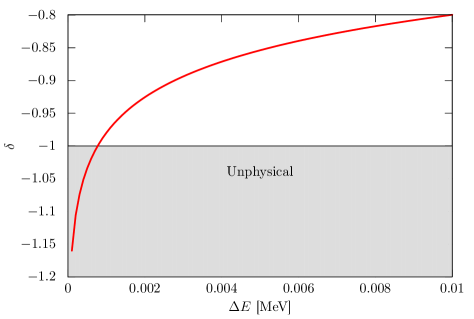
However, figure 5.6 reveals that $\delta$ diverges to negative infinity in the limit where $\Delta E$ is taken to 0. The first sign of trouble is when $\delta$ becomes less than -1. The multiplicative correction factor $(1+\delta)$ is now negative, implying a negative cross section, which obviously is unphysical. In this case, our perturbative expansion is breaking down. For very small cut-off values, higher order terms start to matter a lot. The probability of the emission of many infinitesimally soft photon is infinite.

Yennie, Frautschi and Suura demonstrated that higher order terms could be taken into account properly by replacing the factor $(1+\delta)$ with $\exp(\delta)$ [94]. The cut-off $\Delta E$ is reinterpreted as the sum of the energy of all of the emitted soft photons. This technique is called exponentiation. Yennie et al. proved that exponentiation is correct in the soft limit, i.e. $\Delta E$ is small and none of the soft photons make an appreciable change in the charged particle kinematics. At larger $\Delta E$, $\delta$ becomes small so that $\exp(\delta)$ becomes quite similar to $(1+\delta)$. At large values of $\Delta E$, the assumptions needed for exponentiation break down.

Exponentiation is a tool that plays key role in the OLYMPUS radiative generator, described in the following sections.

5.3 OLYMPUS Radiative Corrections

5.3.1 Simulating Radiative Corrections with Monte Carlo

Previous radiative corrections approaches are best suited to single-arm measurements with high momentum resolution and well-defined acceptance apertures. OLYMPUS does not have any of these qualities. OLYMPUS is a coincidence experiment: proton detection is built in to the trigger. The OLYMPUS spectrometer has a large continuous angular acceptance, but poor momentum resolution. The acceptance is complicated since the OLYMPUS target is not-point like.

An alternative approach is to use Monte Carlo simulation. In this approach, elastic $ep$ and bremmstrahlung events are randomly generated—that is, the momentum vectors of the outgoing particles are assigned—according to radiatively corrected cross sections. These events form the input of the OLYMPUS simulation software, which simulates particle trajectories through the magnetic field and through the matter of the detectors and simulates the signals that would be produced in the detectors. Rather than making a correction to a measurement, in this approach the measurement is compared with that from the simulated data set.

This approach requires a great deal of software infrastructure. However it brings two advantages. The first is that all of the complicated convolutions between radiative corrections, detector acceptance, and reconstruction efficiency are handled automatically. The second is flexibility in event selection. To use previous radiative corrections schemes, one’s elastic event selection must be limited to picking a value for $\Delta E$ of the lepton (or $W$ using Ent et al.). But by using a simulation, one can select elastic events with any cuts one wants and apply them to both the measured and simulated data sets. This flexibility is necessary for a coincidence experiment like OLYMPUS, since proton information plays a vital role in segregating elastic events from background.

The first step in this chain is to produce randomly generated events according to a cross section that has been radiatively corrected. Software for this purpose is called a “radiative event generator.” This task isn’t completely straightforward; there are several design choices and approximations that must be made. The rest of this section will cover the specifics of the OLYMPUS radiative event generator.

Using Monte Carlo to simulate radiative corrections is not new with OLYMPUS. In fact, in high-energy particle physics this approach is now universal, and there are many widely distributed radiative generators for high energy processes. For the OLYMPUS experiment, we wrote an entirely new generator as a way to guarantee that the priorities and features matched our needs. In parallel to our work, the Novosibirsk two-photon experiment also wrote a brand new elastic $ep$ event generator, called ESEPP, described in a recent work [95]. I will not cover ESEPP in detail in this thesis, but I will note that it was used to test the OLYMPUS generator during its development.

5.3.2 OLYMPUS Radiative Event Generator

A new radiative event generator was written specifically for OLYMPUS. Though this required a great deal of work, which wouldn’t have been necessary had we used an alternative suitable generator, such as ESEPP, it did give us full understanding and control of what was going on “under the hood.” Additionally we were able to build in features that were well-suited to the OLYMPUS analysis.

The most important of these features was the ability to have multiple weights. The OLYMPUS generator is a weighted generator: each event carries a scalar weight describing its contribution to the Monte Carlo integral. As a brief example, let’s consider a generator which produces samples of a random variable $x$ aiming to reproduce a cross section $d\sigma/dx$. The generator might sample $x$ according to a probability distribution $P(x)$, in which case each event will carry a weight of $d\sigma/dx\times(1/P(x))$. For the OLYMPUS analysis, we wanted to simulate several different radiative correction models, and ordinarily this would require simulating the data set multiple times. The generation step is quite fast relative to the simulation of how tracks propagate through the detector, and much faster compared to the track reconstruction. Therefore, we designed the OLYMPUS generator so that each event carried a list of weights, one for each radiative corrections model we wanted to test. In the language of our earlier example, the list would have weights: $\{d\sigma_{1}/dx\times(1/P(x)),d\sigma_{2}/dx\times(1/P(x)),d\sigma_{3}/dx\times(1/P(x))\ldots\}$. At the end-stage of the simulation, all of the events could be reweighted to get the results for each model without having to re-propagate or re-track.

The radiative corrections choice with the biggest potential to affect the OLYMPUS result is whether or not to use exponentiation. For that reason, we have two big classes of weights. In what we call “Method 1” we extrapolate a soft exponentiated correction from the elastic peak out to large values of bremsstrahlung photon energy. In what we call “Method 2”, we define a small arbitrary region of kinematic space around the elastic peak. Inside that region, we treat the event as fully elastic and use a non-exponentiated soft correction. Outside that region, we use the tree-level bremsstrahlung cross section. You can see that both methods are more complicated than simply using exponentiation or not. However, in short hand, it will be convenient to refer to Method 1 as the exponentiating method, and Method 2 as the non-exponentiating method.

I should note that Method 1 borrows heavily from the radiative corrections procedure developed by Jan Bernauer for the A1 collabaration at Mainz, a description of which can be found in chapter 5 of his thesis [96]. Method 1 is not a pure reproduction of the A1 generator in all areas, but follows some aspects exactly, namely the prescription for the radiative cross section and the sampling of the photon direction.

In this section, I will first describe our derivation of the radiative cross section used by Method 1. Next, I will describe our choice of probability distribution for sampling the kinematic variables, since this is important for guaranteeing good numerical behavior for Method 1. Then I will explain the cross section used for Method 2.

Method 1: Exponentiation

The quandary with exponentiation is that, while it provides a prescription for accounting for radiation to all orders, it only does so in the soft limit; that is, when the amount of energy radiated away by bremsstrahlung photons is small. When a large amount of energy has been radiated away, it makes more sense to think of the cross section in terms of that for hard bremsstrahlung. The prescription of method 1 attempts to interpolate between these two regions in a continuous way.

To begin the derivation, let’s start by describing what an ideal solution would look like. In OLYMPUS, the scattered lepton and recoiling proton are detected in coincidence. Therefore, the ideal cross section would be of the form:

$$\frac{d^{6}\sigma}{d\vec{p_{l}}d\vec{p_{p}}},$$

where there is dependence on both the lepton momentum vector and the proton momentum vector. And ideally, this cross section would account for radiative corrections to all orders. We do not have a prescription for such an ideal cross section, so we will have to make some assumptions in order to approximate it.

The first practical assumption we can make is that the ideal cross section is dominated deep in the tail by hard single-photon bremsstrahlung. Single photon bremstrahlung has a 3-body final state (lepton, proton, and photon), and therefore occupies a 5-dimensional kinematic space. Our first assumption is that we can reduce our six-fold differential cross section to a five-fold differential cross section; that is, by fixing five kinematic variables, we’ve uniquely specified the kinematics of the final state. We can choose to fix any five independent variables. For this generator, our choice of five will be two for the lepton solid angle, $\Omega_{l}$: ($\cos\theta_{l},\phi_{l}$), two for the photon solid angle, $\Omega_{\gamma}$: ($\cos\theta_{\gamma},\phi_{\gamma}$), and the energy loss of the lepton $\Delta E_{l}=E_{l}^{\text{el.}}-E_{l}$. We will specify a cross section of the form:

$$\frac{d^{5}\sigma}{d\Omega_{l}d\Omega_{\gamma}d\Delta E}.$$

We can choose to write this differential cross section in the following way:

$$\frac{d^{5}\sigma}{d\Omega_{l}d\Omega_{\gamma}d\Delta E} =\frac{\partial^{3}}{\partial\Omega_{\gamma}\partial\Delta E_{l}}\left[\frac{d\sigma}{d\Omega_{l}}_{1\gamma}e^{f(\Omega_{\gamma},\Delta E_{l}|\Omega_{l})}\right]$$ (5.6)

$$=\frac{d\sigma}{d\Omega_{l}}_{1\gamma}e^{f}\left[\frac{\partial^{3}f(\Omega_{\gamma},\Delta E_{l}|\Omega_{l})}{\partial\Omega_{\gamma}\partial\Delta E_{l}}\right],$$ (5.7)

where the one-photon elastic cross section has been factored out, and the dependence on $\Omega_{\gamma}$ and $\Delta E_{l}$ is contained in an undetermined function $f(\Omega_{\gamma},\Delta E_{l}|\Omega_{l})$. The point of writing the cross section in this form is to make an explicit connection to how a standard radiative correction is applied (with exponentiation). The function $f$ takes the place of $\delta$. The dependence on $\Delta E_{l}$ in a standard correction comes from integrating over the bremsstrahlung cross section with the elastic cross section factored out:

$$\delta(\Delta E_{l}|\Omega_{l})=\left(\frac{1}{\frac{d\sigma}{d\Omega_{l}}_{1\gamma}}\right)\int_{0}^{\Delta E_{l}}d\Delta E_{l}^{\prime}\int_{4\pi}d\Omega_{\gamma}\frac{d^{5}\sigma}{d\Omega_{l}d\Omega_{\gamma}d\Delta E_{l}^{\prime}}_{\text{brems.}},$$ (5.8)

so that by differentiating with respect to energy, we get:

$$\frac{\partial\delta}{\partial\Delta E_{l}}=\left(\frac{1}{\frac{d\sigma}{d\Omega_{l}}_{1\gamma}}\right)\int_{4\pi}d\Omega_{\gamma}\frac{d^{5}\sigma}{d\Omega_{l}d\Omega_{\gamma}d\Delta E_{l}}_{\text{brems.}}.$$ (5.9)

A standard $\delta$ has no dependence on $\Omega_{\gamma}$, since this is integrated out. But this brings us to our second assumption, that we can approximate the derivatives of our underdetermined function $f$ with the tree-level bremsstrahlung cross section:

$$\left[\frac{\partial^{3}f(\Omega_{\gamma},\Delta E_{l}|\Omega_{l})}{\partial\Omega_{\gamma}\partial\Delta E_{l}}\right]\longrightarrow\left(\frac{1}{\frac{d\sigma}{d\Omega_{l}}_{1\gamma}}\right)\frac{d^{5}\sigma}{d\Omega_{l}d\Omega_{\gamma}d\Delta E_{l}}_{\text{brems.}}.$$ (5.10)

Putting this back into equation 5.7, we get:

$$\frac{d^{5}\sigma}{d\Omega_{l}d\Omega_{\gamma}d\Delta E}=e^{f}\frac{d^{5}\sigma}{d\Omega_{l}d\Omega_{\gamma}d\Delta E_{l}}_{\text{brems.}}.$$ (5.11)

Our third and final assumption is that we can replace $f$ in $e^{f}$ with a standard correction $\delta$ of our choosing. That brings us to the expression for the Method 1 cross section:

$$\frac{d^{5}\sigma}{d\Omega_{l}d\Omega_{\gamma}d\Delta E}=e^{\delta}\frac{d^{5}\sigma}{d\Omega_{l}d\Omega_{\gamma}d\Delta E_{l}}_{\text{brems.}}.$$ (5.12)

In Method 1, there are a few things to consider. First, this approach works only in the near-elastic limit. Exponentiation is only valid in this limit, and in addition, standard corrections all use the “Soft-Photon Approximation”, which assumes that so little energy is carried away by bremsstrahlung photons that the elastic scattering matrix element can be analytically factored out of the bremsstrahlung matrix element. It is a mistake to trust that this cross section will be accurate deep in the radiative tail. Second, this method aims to account for radiation to all orders, but uses a single-photon bremsstrahlung cross section to predict the dependence on $\Omega_{\gamma}$. This assumption is probably pretty good because the bremsstrahlung cross section blows up for very soft emitted photons. If multiple photons are emitted summing to a total energy of $E_{\gamma}$, then the dominant mode will be one photon carrying nearly $E_{\gamma}$, with all other photons being soft. Third, for near-elastic kinematics, $\delta$ is negative, but increases with increasing $\Delta E_{l}$. $e^{\delta}$ is a suppression factor for the bremsstrahlung cross section and implies that higher-order radiative effects slightly reduce what we’d expect for the bremsstrahlung cross section. For very large values of $\Delta E_{l}$, i.e., far from the elastic peak, $\delta$ will cross over and become positive, and $e^{\delta}$ is an enhancement factor. As mentioned earlier, the region deep in the tail should not be trusted. In the same way, an enhancement of bremsstrahlung in the deep tail is not necessarily believable. If our result depends on events in these kinematics, then Method 1 is probably not a good prescription for us.

Sampling Distribution

Now that we have a prescription for our radiatively-corrected cross section, all that a radiative generator needs to do is to produce random samples of the variables $(\cos\theta_{l},\phi_{l},\cos\theta_{\gamma},\phi_{\gamma},\Delta E_{l})$ and then to weight each event $i$ with weight $w_{i}$:

$$w_{i}=\frac{e^{\delta}}{P(\cos\theta_{l},\phi_{l},\cos\theta_{\gamma},\phi_{\gamma},\Delta E_{l})}\frac{d^{5}\sigma}{d\Omega_{l}d\Omega_{\gamma}d\Delta E_{l}}_{\text{brems.}},\$$ (5.13)

where $P$ is the probability distribution that is being sampled. In an ideal world of infinite computing power, the choice of $P$ does not affect the accuracy of the generator. However, from a practical standpoint, the choice of $P$ can have a large impact on the performance of the generator. There are three issues to keep in mind.

1. Weight uniformity: The simulated data will eventually be binned according to some set of criteria, and the weights of the events in the bin will be summed. The statistical uncertainty in the bin contents for a given Monte Carlo sample is proportional to the variance of the weights of the events in the bin. If the choice of $P$ produces a large variance in weights, then more simulated data will be needed to attain equivalent precision.

2. Ease of sampling: If sampling from $P$ is computationally difficult, then the generator will be slower and the simulation will have less precision for an equivalent run time.

3. Numerical stability: If the weights or components needed for calculating the weights get very large or very small, care must be taken to avoid numerical instability. A careful choice of $P$ may help reduce instability.

To make the weights completely uniform, all one needs to do is sample from a distribution that is proportional to the underlying cross section. However, this is often computationally difficult. The underlying cross section is also highly non-uniform. The cross section varies strongly with $\cos\theta_{l}$, has an integrable divergence as $\Delta E_{l}\longrightarrow 0$, and has a non-trivial dependence on $\Omega_{\gamma}$. In short, there are many opportunities for numerical instability. Keeping these concerns in mind, let’s look at the OLYMPUS radiative generator’s choice of $P$.

First, the cross section is fully azimuthally symmetrical, so $\phi_{l}$ can be sampled isotropically. We choose also to sample $\cos\theta_{l}$ isotropically since we are interested in results as a function of $\theta_{l}$. Even though weights will vary significantly over the range of $\theta_{l}$, we will usually be binning by $\theta_{l}$ (or by some monotonically related variable, like $Q^{2}$), so we will not be introducing a large variance into any individual bin. Once we have chosen $\cos\theta_{l}$ and $\phi_{l}$, then we can work on sampling $\Delta E_{l}$.

For $\Delta E_{l}$, we want a sampling distribution that matches the cross sections dependence on $\Delta E_{l}$, given the constraints of numerical stability and ease of computation. Fortunately, we know that the $\Delta E_{l}$ dependence is approximately $\exp{\delta}\frac{\partial\delta}{\partial\Delta E_{l}}$, so we can use this as our sampling distribution. In just about every standard correction, $\delta$ takes the form

$$f+\frac{t}{2}\log\left[u\left(\frac{\Delta E_{l}}{E^{\text{el.}}}\right)^{2}\right]$$ (5.14)

for some constants $f$,$t$,$u$ that depend on the lepton angle. Our probability distribution will be:

$$P(\Delta E_{l}|\Omega_{l})\sim e^{\delta}\frac{\partial}{\partial\Delta E}\left\{f+\frac{t}{2}\log\left[u\left(\frac{\Delta E_{l}}{E^{\text{el.}}}\right)^{2}\right]\right\}$$ (5.15)

$$\sim e^{f}\left[u^{t/2}\left(\frac{\Delta E_{l}}{E^{\text{el.}}}\right)^{t}\right]\frac{t}{u\Delta E_{l}}$$ (5.16)

$$\sim \left(\Delta E_{l}\right)^{t-1},$$ (5.17)

that is, a power law. To determine the normalization, let’s integrate over the range $[0,\Delta E_{\text{cut}}]$:

$$1= N\int_{0}^{\Delta E_{\text{cut}}}\left(\Delta E_{l}\right)^{t-1}$$ (5.18)

$$= \frac{N\left(\Delta E_{\text{cut}}\right)^{t}}{t}$$ (5.19)

$$N= \frac{t}{\Delta E_{\text{cut}}^{t}}$$ (5.20)

$$P(\Delta E_{l}|\Omega_{l})= \frac{t}{\Delta E_{l}}\left(\frac{\Delta E_{l}}{\Delta E_{\text{cut}}}\right)^{t}$$ (5.21)

Let’s take a look at what the event weights will be. Of course, we haven’t yet specified $P(\Omega_{\gamma}|\Omega_{l}\Delta E_{l})$, but we can start to get an idea. In appendix A, the tree-level bremsstrahlung cross section is worked out. Specifically, we’ll need the result in equation A.49. When we combine all of the elements, we find that the weight for an event with kinematics ($\Omega_{l}$, $\Omega_{\gamma}$, $\Delta E_{l}$) is:

$$w =e^{\delta}\times\frac{d^{5}\sigma}{d\Omega_{l}d\Omega_{\gamma}d\Delta E_{l}}_{\text{brems.}}\times\frac{1}{P(\Omega_{l})P(\Delta E_{l}|\Omega_{l})P(\Omega_{\gamma}|\Omega_{l}\Delta E_{l})}$$ (5.22)

$$=e^{f}u^{t/2}\left(\frac{\Delta E_{l}}{E_{3}^{\text{el.}}}\right)^{t}\frac{\alpha^{3}\left\langle|\mathcal{M}^{\prime}|^{2}\right\rangle}{64\pi^{2}E_{1}m_{p}}\frac{E_{3}}{\left|E_{4}+E_{3}+k\cos\theta_{l\gamma}-E_{1}\cos\theta_{l}\right|}\frac{\tilde{\mathcal{J}}}{\Delta E_{l}}\frac{\frac{\Delta E_{l}}{t}\left(\frac{\Delta E_{l}}{\Delta E_{\text{cut}}}\right)^{-t}}{P(\Omega_{l})P(\Omega_{\gamma}|\Omega_{l}\Delta E_{l})}$$ (5.23)

$$=\frac{e^{f}u^{t/2}}{t}\left(\frac{\Delta E_{\text{cut}}}{E_{3}^{\text{el.}}}\right)^{t}\frac{\alpha^{3}\left\langle|\mathcal{M}^{\prime}|^{2}\right\rangle}{64\pi^{2}E_{1}m_{p}}\frac{E_{3}}{\left|E_{4}+E_{3}+k\cos\theta_{l\gamma}-E_{1}\cos\theta_{l}\right|}\frac{\tilde{\mathcal{J}}}{P(\Omega_{l})P(\Omega_{\gamma}|\Omega_{l}\Delta E_{l})}.$$ (5.24)

The problematic divergence of the type $(\Delta E_{l})^{-1}$ from the cross section has been cancelled by the factor of $\Delta E_{l}$ in the sampling distribution. Our weight will be numerically stable, even for small values of $\Delta E_{l}$.

Fortunately, it is very easy to produce random numbers in a power law distribution. To produce random numbers in the distibution $P(\Delta E_{l}|\Omega_{l})$, we’ll need to invert the cumulative distribution $C(\Delta E_{l}|\Omega_{l})=(\Delta E_{l}/\Delta E_{\text{cut}})^{t}$. Given a random number $r$, uniformly sampled on $[0,1]$, then:

$$\Delta E_{l}=\Delta E_{\text{cut}}r^{1/t}.$$ (5.25)

Figure 5.7: The bremsstrahlung cross section for fixed $\theta_{l}=10^{\circ}$, $\Delta E_{l}=100$ MeV is plotted as a function of the photon angles. The cross section is strongly peaked in the direction of the incoming electron ($0^{\circ},0^{\circ}$) and the outgoing electron ($10^{\circ},0^{\circ}$). The generator will have the best performance if the photon angle sampling distribution matches those peaks.

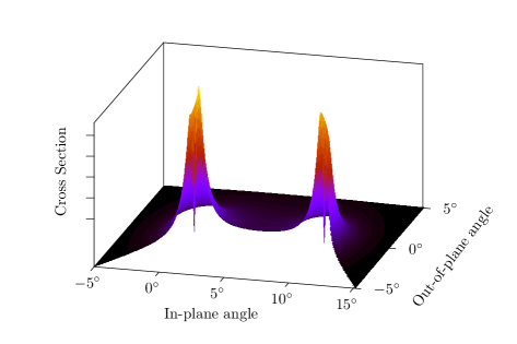
The final piece of the sampling distribution is the photon direction distribution, $P(\Omega_{\gamma}|\Omega_{l},\Delta E_{l})$. The photon direction distribution in bremsstrahlung has two very large peaks: one in the same direction as the beam momentum, the other in the direction of the scattered lepton’s momentum. These can be seen in figure 5.7. In experiments at higher energies than OLYMPUS, bremsstrahlung can also be peaked in the direction of the recoiling proton, though the high mass of the proton broadens this peak.

The highly-peaked nature of the bremsstrahlung distribution can pose problems for our radiative generator. If we sample the photon direction isotropically, the large change in cross section will produce a large variance in weights, hurting the generator performance. Since in every analysis we do, we integrate out the photon direction, we want to sample from a distribution that matches the cross section as closely as possible. However, sampling from the cross section directly is difficult because we can’t invert, and because it is fairly computationally difficult to calculate it. It’s feasible to calculate it a few times per event to produce a weight; it is not feasible to calculate it thousands of times per event.

Our solution (illustrated in figure 5.8), is to model two peaks in the angular distribution with the function:

$$P(\cos\theta) =\frac{1}{2\frac{E_{l}}{p_{l}}\log\left[\frac{E_{l}+p_{l}}{E_{l}-p_{l}}\right]-4}\times\frac{1-\cos^{2}\theta}{\left(\frac{E_{l}}{p_{l}}-\cos\theta\right)^{2}}$$ (5.26)

$$=\frac{1}{N}\times\frac{1-\cos^{2}\theta}{\left(\frac{E_{l}}{p_{l}}-\cos\theta\right)^{2}},$$ (5.27)

where $\theta$ is the angle between the photon and lepton, $E_{l}$ is the energy of the lepton, and $p_{l}$ is the norm of the three-momentum of the lepton ($E_{l}$ is very nearly equal to $p_{l}$). Sampling from this distribution requires us to invert the cumulative distribution:

$$C(\cos\theta)=\frac{1}{N}\int_{-1}^{1}d\cos\theta\frac{1-\cos^{2}\theta}{\left(\frac{E_{l}}{p_{l}}-\cos\theta\right)^{2}}.$$ (5.28)

Let’s substitute $x=\frac{E_{l}}{p_{l}}-\cos\theta$:

$$C(\cos\theta) =\frac{1}{N}\int_{\frac{E_{l}}{p_{l}}-1}^{\frac{E_{l}}{p_{l}}-\cos\theta}\frac{dx}{x^{2}}\left[\left(1-\frac{E_{l}}{p_{l}}^{2}\right)+2\frac{E_{l}}{p_{l}}x-x^{2}\right]$$ (5.29)

$$=\frac{1}{N}\left[\left(1-\frac{E_{l}}{p_{l}}^{2}\right)\left\{\frac{1}{\frac{E_{l}}{p_{l}}-1}-\frac{1}{\frac{E_{l}}{p_{l}}-\cos\theta}\right\}+2\frac{E_{l}}{p_{l}}\log\left\{\frac{\frac{E_{l}}{p_{l}}-\cos\theta}{\frac{E_{l}}{p_{l}}-1}\right\}+\cos\theta-1\right]$$ (5.30)

$$=\frac{1}{N}\left[\cos\theta+2\frac{E_{l}}{p_{l}}\log\left\{\frac{\frac{E_{l}}{p_{l}}-\cos\theta}{\frac{E_{l}}{p_{l}}-1}\right\}-2-\frac{E_{l}}{p_{l}}-\frac{\left(1-\frac{E_{l}}{p_{l}}^{2}\right)}{\frac{E_{l}}{p_{l}}-\cos\theta}\right].$$ (5.31)

This can be inverted numerically using bisection.

Figure 5.8: The bremsstrahlung cross section (top plot) varies over several orders of magnitude with respect to the photon direction. We sample the photon direction from the distribution shown in the middle plot. The resulting weights (bottom plot) are much more uniform.

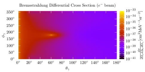
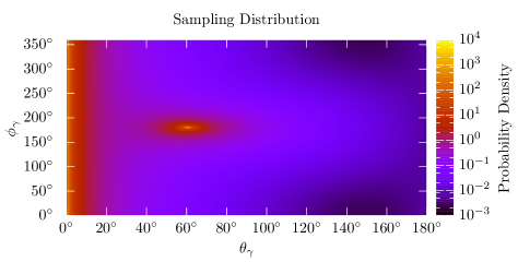
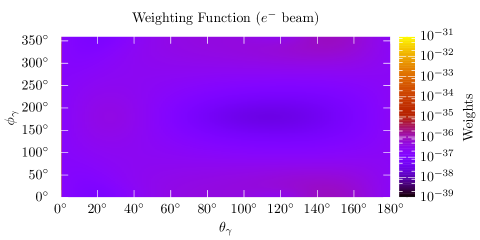
Our approach on each event is to pick either the incoming lepton or the outgoing lepton with equal probability. Then we sample $\cos\theta$ as described above, while we sample $\phi$ isotropically. We then must transform these angles from the coordinate system relative to lepton to the global coordinate system. With five kinematic variables now fixed, the kinematics of the entire event are determined. We can specify the four-vectors for all of the incoming and outgoing particles and can calculate all of the components needed to form the weight in equation 5.24.

Method 2: Non-Exponentiation

An alternative approach to Method 1 is to avoid using exponentiation, and to simply aim to produce a cross section that is accurate at next-to-leading order. The advantage is that the problems with extrapolating an exponentiated correction far from the elastic peak are avoided, but the cost is that radiation is not treated to all orders. The non-exponentiated approach was added to the OLYMPUS radiative generator as an alternate weight, and is known as Method 2. This was largely the work of my classmate Rebecca Russell, who deserves, if not all of the credit, at least all minus $\epsilon$.

Method 2 weights are calculated for each event, along with method 1 weights. That means that Method 2 has to make do with the same sampling distribution as described in the previous section. This posed some minor complications, for which effective solutions have been found.

Method 2 works by segregating events into those it considers elastic, and those it considers inelastic. The segregation criterion is the energy emitted by the bremsstrahlung photon, $k$. If the photon energy is less than some arbitrary boundary $k_{b}$, then the event is considered elastic, and given weight:

$$w_{\text{el.}}=\frac{d\sigma}{d\Omega_{l}}_{1\gamma}\times(1+\delta(k_{b}))\times\frac{1}{P(\Omega_{l},\Omega_{\gamma},\Delta E_{l})}.$$

If $k>k_{b}$, then the event is considered inelastic, and given weight:

$$w_{\text{inel.}}=\frac{d\sigma}{d\Omega_{l}d\Omega_{\gamma}d\Delta E_{l}}_{\text{brems.}}\times\frac{1}{P(\Omega_{l},\Omega_{\gamma},\Delta E_{l})}.$$

Elastic events are essentially weighted according to a standard correction, and inelastic events are weighted according to the tree-level bremsstrahlung cross section. Radiative effects at the next-to-leading level are reproduced. The choice of boundary $k_{b}$ should not have an effect on the result. It must be chosen to be much smaller than the detector resolution, but larger than the point at which $\delta$ becomes negative (see figure 5.6). Typically, we chose $k_{b}=1$ MeV.

This method runs into trouble because the so-called elastic events have a large variance in their weights. To make Method 1 work, we sampled the photon angle from a sharply peaked distribution. The cross section for these events, $(1+\delta)d\sigma/d\Omega$ has no dependence on the photon direction. Dividing by the sampling distribution produces an enormous variance.

To make Method 2 work, individual elastic weights were replaced by average elastic weights:

$$w_{\text{el.}}\longrightarrow\langle w_{\text{el.}}\rangle=\frac{d\sigma}{d\Omega_{l}}_{1\gamma}\int_{k<k_{b}}P(\Omega_{\gamma},\Delta E_{l}|\Omega_{l})d\Omega_{\gamma}d\Delta E\frac{(1+\delta(k_{b}))}{P(\Omega_{\gamma},\Delta E_{l}|\Omega_{l})}.$$

These average elastic weights were precomputed for a wide range of lepton angles. When computing a weight, the generator would interpolate between precomputations at the nearest scattering angles. This significantly reduced the variance in the weights.

Another minor complication comes from the choice of elasticity criterion. Most standard corrections define $\delta$ as a function of $\Delta E_{l}$, the energy lost by the lepton relative to elastic energy. In a coincidence measurement, the photon energy $k$, which is equivalent to the missing energy $W$, makes more sense as an elasticity criterion. To make Method 2 work, a correction $\delta(k)$ was needed. Ent et al. describe such a formulation [93], but neglect the electron mass. Gramolin et al., in their description of the ESEPP generator, describe a prescription that, while not analytic, does preserve the electron mass [95]. The OLYMPUS generator follows the ESEPP prescription.

We also chose a third alternate weight using $\Delta E_{l}$ as the elasticity criterion. We refer to this as “Method 3”, though this method is philosophically identical to Method 2, and should probably have been named “Method 2a.” The use of $\Delta E_{l}$ as the elasticity criterion greatly simplifies the algebra, but can produce somewhat undesirable effects. For instance, it is possible for events with a large photon energy to be considered elastic, simply because the proton has lost energy, not the lepton. Still, this method costs almost nothing, so we chose to add it to our ensemble of weights. The average weight in the elastic region is trivial:

$$\langle w_{\text{el.}}\rangle =\frac{d\sigma}{d\Omega_{l}}_{1\gamma}\int_{4\pi}d\Omega_{\gamma}\int_{0}^{\Delta E_{b}}d\Delta E_{l}P(\Omega_{\gamma},\Delta E_{l}|\Omega_{l})\frac{(1+\delta(\Delta E_{b}))}{P(\Omega_{\gamma},\Delta E_{l}|\Omega_{l})}$$ (5.32)

$$=4\pi\Delta E_{b}(1+\delta(\Delta E_{b})).$$ (5.33)

5.4 Discussion

Figure 5.9: Events from the generator are binned by the lepton angle and the lepton momentum. The top plot shows the cross section produced with an electron beam. The bottom plot shows the ratio of positron and electron cross sections. The kinematic dependence of the ratio is non-trivial.

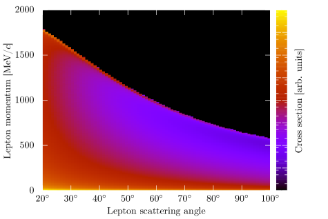
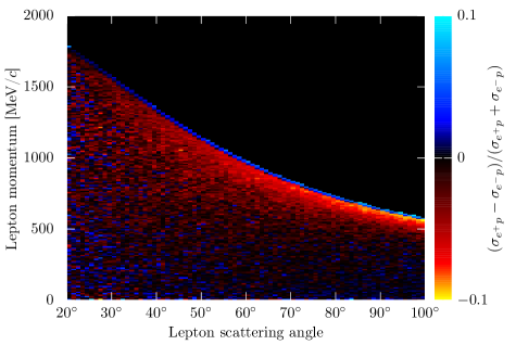
Plots of the generator output are shown in figure 5.9, histogrammed by lepton angle and momentum. Of course, the generator cross section is five-dimensional, but for the purposes of visualization, I’ve had to choose two variables. In these plots, the elastic ridge is the top of the colored region, above which the kinematics are forbidden. The top plot shows the cross section with an electron beam. There is considerable cross section for very low photon momenta at all photon angles. This is caused by initial state radiation, which will be discussed in subsection 5.4.3. The bottom plot shows the ratio of the positron-proton cross section to the electron-proton cross section. The ratio varies significantly over the kinematic range shown, and does so in a non-trivial way. Close to the elastic ridge, positrons are favored; further in the tail, electrons are favored. If the generator has any errors in its implementation, it would be very easy to influence the ratio in a spurious way.

We took a number of steps to validate the radiative generator, and I will discuss some of these in this section. The most complicated part of the generator, the bremsstrahlung matrix element, was validated against that of the ESEPP generator. The generator output was also tested against the radiative tails from standard radiative corrections.

5.4.1 Matrix Element Comparison with ESEPP

The bremsstrahlung matrix element was a very large source of potential bugs. As a cross check, we compared our matrix element against that of the ESEPP generator. Our two different implementations of the matrix element should give the exact same results (up to the choice of definition for the off-shell proton current, a very minor effect). Our initial comparisons revealed some typing mistakes on our part, and after fixing these, our matrix elements agreed to a very high level. Our lepton terms, which have no off-shell proton vertices, agreed to the level of the numerical precision of our computer, and the proton term and interference term agreed to better than one part in $10^{5}$. After this, we were satisfied that our matrix element implementation was correct.

5.4.2 Comparisons with Maximon and Tjon

After we had confidence in our implementation of bremsstrahlung, we then turned to the task of verifying the generator as a whole. One straightforward test is to use the generator to integrate over the photon direction and compare the result (which depends on $\theta_{l}$, and $\Delta E_{l}$) with the predictions of a standard correction. By default, our generator uses the $\delta$ from Maximon and Tjon, and that particular choice was natural for comparison.

Figure 5.10: Our generator converges to the Maximon and Tjon prediction as $\Delta E_{l}\rightarrow 0$, for both Method 1 (top) and Method 2 (bottom), just as we expect.

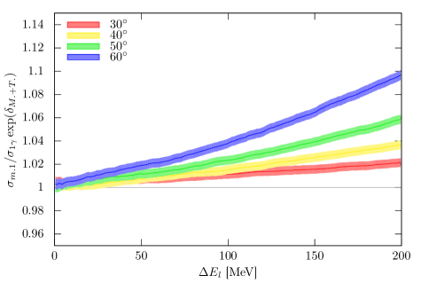
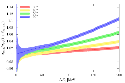
Figure 5.10 shows the results from the generator, divided by the prediction of Maximom and Tjon, plotted as a function of $\Delta E_{l}$. The $y$-axis is the generator cross section, integrated over photon direction and over $\Delta E_{l}$ up to the point marked on the $x$ axis. This is then divided by that same cross section as predicted by Maximon and Tjon. In the case of Method 1 (top plot) we are comparing to an exponentiated $\delta$, and in the case of Method 2 (bottom plot) we are comparing to a non-exponentiated $\delta$. The results confirm that the generator is behaving as expected. Both Method 1 and Method 2 converge to Maximon and Tjon when $\Delta E_{l}$ is small, for multiple angles. We expect convergence at low $\Delta E_{l}$ because Maximon and Tjon (and all standard corrections) calculate bremsstrahlung in the soft limit. When the energy carried away by the bremsstrahlung photon becomes large (and consequently $\Delta E_{l}$ grows), Maximon and Tjon become less accurate (compared with the full tree-level calculation in our generator.)

It is noticeable that, for very small values of the $\Delta E_{l}$ cut-off, the uncertainty from Method 2 increases substantially. This is caused by the sampling distribution. The uncertainty is driven by how many samples fall within Method 2’s elastic region.

Figure 5.11: The cross section ratio predicted by the generator is almost identical to that predicted by Maximon and Tjon, and it’s largely insensitive to the $\Delta E_{l}$ cut-off.

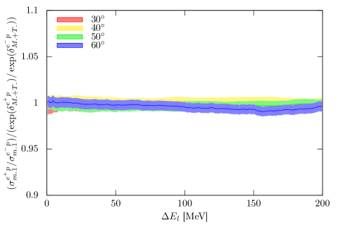
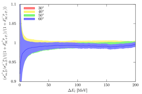
The goal of OLYMPUS is to compare electrons and positrons, so we must also compare the behavior of the generator with respect to both lepton species. Figure 5.11 shows the cross sectio ratio predicted by the generator divided by that predicted by Maximon and Tjon. As expected, both methods converge to Maximon and Tjon for small values of the $\Delta E_{l}$ cut-off (although the uncertainty of Method 2 is large for very small cut-off values). What is also reassuring is that the agreement is largely independent of $\Delta E_{l}$. The magnitude of the radiative correction introduced into the positron-electron ratio by our generator will not deviate from Maximon and Tjon regardless of the effective $\Delta E_{l}$ cut-off used in our analysis.

Figure 5.12: Method 2 and Method 1 are very similar for large cut-off values. The differences between the two methods are only large at very small cut-off values. The effective cut-off for OLYMPUS will probably be on the order of 100–200 MeV.

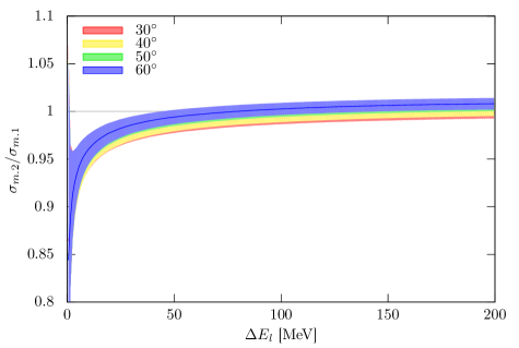
We can also ask how Method 1 and Method 2 compare with each other as a function of angle and cut-off. The ratio of the two corrections is shown in figure 5.12. At large values of the $\Delta E_{l}$ cut-off, Method 1 and Method 2 converge. This makes sense. As $\Delta E_{l}$ grows, $\delta$ gets closer to 0, and in that limit, there is little difference between $\exp(\delta)$ and $(1+\delta)$. There are some persistent differences at the percent-level. These differences will inform our systematic uncertainty from radiative corrections.

5.4.3 Enhancement Due to Initial State Radiation

There is interesting behavior in figure 5.10: the generator cross section rises relative to Maximon and Tjon with increasing $\Delta E_{l}$. This implies that the generator cross section has a heavier radiative tail than Maximon and Tjon predict. Figure 5.13 shows the radiative tails predicted by Method 1 (bins), as well as those of Maximon and Tjon (lines). I could, in principle, show Method 2 as well, but the differences are imperceptible on a log scale. The radiative tails are fatter in the generator than in Maximon and Tjon.

Figure 5.13: The cross section increases at large values of $\Delta E_{l}$ because of initial state radiation. Bremsstrahlung from the initial lepton leg effectively reduces the incoming beam energy, enhancing the cross section.

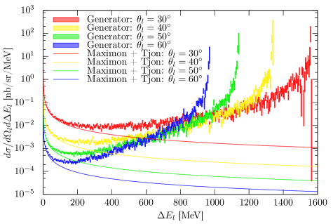
What is even more surprising is that the cross section reaches a minimum and then starts rising. It continues to rise all the way to the maximum value: $\Delta E_{l}=E_{3}^{\text{el.}}-m_{e}$. The origin of this phenomenon is initial state radiation (ISR). If the bremsstrahlung photon is emitted in the incoming lepton direction, the dominant diagram is the one where the photon is emitted from the initial lepton leg. The photon carries energy away from the lepton, effectively reducing the beam energy. The elastic scattering cross section is larger at smaller beam energies. Our generator, which uses a full tree-level bremsstrahlung matrix element, captures this phenomenon. Maximon and Tjon, which calculates bremsstrahlung in the soft-limit, cannot.

While this was a very satisfying discovery to make, it exposes a potential problem in our sampling distribution. To make our weights uniform, we sampled $\Delta E_{l}$ according to Maximon and Tjon (the lines in figure 5.13), aiming to reproduce the distribution predicted by generator’s cross section (bins in figure 5.13). Since the two distributions diverge, the weights will become increasingly large as $\Delta E_{l}$ increases. If we were ever to do a study in which we integrated over the full range of $\Delta E_{l}$, there would be an enormous variance in the weights. Now certainly an elastic event selection will reject events with large $\Delta E_{l}$, and so any use of the simulation for such studies will not be hampered by weight variance. However, we tried to devise a solution in case any simulations deep in the tail were needed.

Our solution is to add a second sampling distribution for $\Delta E_{l}$ that rises with $\Delta E_{l}$, in order to capture the ISR enhancement. We propose modifying the sampling distribution:

$$P(\Delta E_{l}|\Omega_{l})\longrightarrow\chi\frac{t}{\Delta E_{l}}\left(\frac{\Delta E_{l}}{\Delta E_{\text{cut}}}\right)^{t}+(1-\chi)P_{\text{ISR}}(\Delta E_{l}|\Omega_{l}),$$ (5.34)

where the variable $\chi$ represents the fraction of events drawn in the “soft” distribution, while $(1-\chi)$ represents the fraction drawn in the “hard” ISR distribution. What functional form should we then use for $P_{\text{ISR}}(\Delta E_{l}|\Omega_{l})$? The one-photon-exchange cross section scales roughly with $E^{-2}$ at low beam energies. Therefore, a reasonable choice would be:

$$P_{\text{ISR}}(\Delta E_{l}|\Omega_{l})=\frac{E(E-\Delta E_{\text{cut}})}{\Delta E_{\text{cut}}(E-\Delta E_{l})^{2}}.$$ (5.35)

The generator weight will need to be reworked with this new distribution. Whereas before we needed to weight with

$$\frac{1}{P(\Delta E_{l}|\Omega_{l})}=\frac{1}{\frac{t}{\Delta E_{l}}\left(\frac{\Delta E_{l}}{\Delta E_{\text{cut}}}\right)^{t}},$$

we will now need to weight by

$$\frac{1}{P(\Delta E_{l}|\Omega_{l})}= \frac{1}{\frac{\chi t}{\Delta E_{l}}\left(\frac{\Delta E_{l}}{\Delta E_{\text{cut}}}\right)^{t}+(1-\chi)\frac{1}{\frac{t}{\Delta E_{l}}\left(\frac{\Delta E_{l}}{\Delta E_{\text{cut}}}\right)^{t}}}$$ (5.36)

$$= \frac{\Delta E_{l}\left(\frac{\Delta E_{\text{cut}}}{\Delta E_{l}}\right)^{t}}{\chi t+(1-\chi)\frac{E(E-\Delta E_{\text{cut}})}{(E-\Delta E_{l})^{2}}\left(\frac{\Delta E_{l}}{\Delta E_{\text{cut}}}\right)^{1-t}}.$$ (5.37)

Just as before, the numerator is cancelled by factors in the cross section. The second term in the denominator has a bare $\Delta E_{l}^{1-t}$, but since $0<t<1$, this term becomes very small when $\Delta E_{l}$ goes to 0, and thus insignificant compared to the $\chi t$ term. So this modification preserves the numerical stability of the weights.

A useful property with this modification is that $\chi$ is an adjustable parameter for the user. Setting $\chi=1$ restores the unmodified probability distribution, suitable for simulating elastic event selection. Setting $\chi<1$ can increase the number of large $\Delta E_{l}$ events that the generator produces, smoothing out the weights deep in the tail. Described in another way: $\chi$ tunes the statistical precision of the elastic peak versus the ISR peak in a given simulation. Setting $\chi$ close to one enhances the precision of the elastic peak, while setting $\chi$ close to zero gives priority to the ISR peak. $\chi=0.5$ is a middle ground.

5.5 Running the Generator

In this section, I’ll describe the settings used for our simulation of the main analysis. First, the sampling distribution was controlled by two tunable parameters:

1. $\chi=0.5$

2. $\Delta E_{\text{cut}}=E_{3}^{\text{el.}}-m_{e}$, the maximum value at each angle.

We balanced the statistics between the elastic peak and the ISR peak, in case there any ISR events contaminated our elastic event selection. $\Delta E_{\text{cut}}$ was set to the maximum value at each angle; we simulated the entire radiative tail.

Second, each event contained a vector of weights, one for each different cross section model. Broadly these can be categorized as using Method 1 and Method 2; within those categories, there were several choices we could make.

1. Form Factor Models

   • Point-like proton

   • Standard dipole

   • Global fit by Kelly et al. [97]

   • Global fit by Bernauer et al., including $\pm$ fit uncertainties [57]

2. Standard Correction Model

   • Maximon and Tjon [92]

   • Mo and Tsai [89]

   • Meister and Yennie [91]

3. Vacuum Polarization Model

   • Leptonic correction only

   • Leptonic correction + hadronic correction extracted from data [98, 99]

4. Full vs. soft bremsstrahlung

Each combination of all of the different options leads to an individual weight. In analysis, the effect of each choice can be studied be reweighting the simulated histograms. This can be done without resimulating individual events.

Chapter 6 Determining Luminosity from SyMB Multi-Interaction Events

6.1 Introduction

The OLYMPUS data set is technically two data sets: one with an electron beam, the other with a positron beam. In order to make comparisons between the two sets, they both must be normalized by their respective integrated luminosities. OLYMPUS was designed with multiple luminosity monitoring systems with this in mind.

To measure an asymmetry between electron and positron cross sections, strictly speaking, only the relative integrated luminosity between the data sets is needed. It is not crucial that the OLYMPUS luminosity monitors be extremely accurate in their absolute determination of luminosity. It is, however, crucial that the systematic differences in the monitor performance between electron and positron running modes be as small as possible. Uncertainty in the relative luminosity determination between beam species (which I will frequently refer to as “species-relative luminosity” in this chapter) leads directly to uncertainty in the cross section asymmetry that OLYMPUS measures.

OLYMPUS collected data with three independent monitoring systems; the slow control system, the $12^{\circ}$ tracking telescopes, and the symmetric Møller/Bhabha calorimeters (SyMBs). The slow control system, while simple and less accurate, was extremely useful because it could be used online to immediately give a rough estimate of the luminosity of the data being collected. The $12^{\circ}$ telescopes recorded the rate of forward elastic $ep$ scattering from which integrated luminosity could be extracted. This method had an intrinsic limitation due to contributions from hard two-photon exchange. The SyMBs avoided this problem by looking at purely QED processes: Møller and Bhabha scattering. Originally, this detector system was designed to monitor the scattering rate at the symmetric angle by detecting the two final-state leptons in coincidence. After multiple years of analysis, it was found that this method had a systematic uncertainty on the order of 3% for the species-relative luminosity, and thus was not useful for OLYMPUS. However, an alternate analysis method developed by the author—one which makes use of multi-interaction events—was found to have an accuracy better than 0.3%, small enough to be used effectively by OLYMPUS to achieve its physics goals. This alternate analysis, as well as its results, are the subject of this chapter.

6.1.1 Slow Control System

The OLYMPUS slow control system handled the sending of instructions to the myriad of high voltage supplies, vacuum pumps, and gas flow valves, as well as recording the data from a variety of sensors linked to these pieces of equipment. The word “slow” refers to the fact that this sending and recording took place on timescales much slower than the trigger rate. For example, temperature sensors only needed to record variations over time scales of seconds, not microseconds. The data recorded by the slow control system could be used to reconstruct luminosity. The system recorded the beam current in the storage ring, as well as the flow rate of gas into the target and the temperature of the target cell. From this information, the thickness of the target (in units of atoms per area) could be reconstructed, and the luminosity determined.

The slow control system was useful because it was simple. No high-level analysis was needed, and an estimate of luminosity could be determined almost immediately. However, this method lacked the accuracy necessary to make a percent-level asymmetry measurement. In measuring absolute luminosity, the system was estimated to be accurate to the level of 20%, limited mostly by knowledge of the target cell’s gas conductance. Of course, the important figure of merit was the species-relative luminsosity, for which the slow control system was estimated to be accurate to the level of about 3%. The limiting factor was the knowledge of the temperature profile of the gas in the target. Temperature was estimated using a sensor attached to the outside of the target cell, which might have recorded a slightly different temperature than that of the gas inside cell. The gas might also have had a temperature gradient along the length of the cell. Any errors in the gas temperature might have been slightly different for the two beam species. The background environment and beam quality were certainly different between the two species, and this could have altered the equilibrium temperature of the target, either directly, or indirectly through, for example, wake field heating.

6.1.2 $12^{\circ}$ Tracking Telescopes

The $12^{\circ}$ tracking telescopes monitored luminosity by measuring the rate of elastic $ep$ scattering at forward angles. In events of interest, the scattered lepton would pass through the telescope at an approximately $12^{\circ}$ scattering angle, while the recoiling proton would be detected in a time-of-flight scintillator bar on the opposite sector. Most (on the order of 90%) of the protons also passed through the drift chamber acceptance, though this was not a requirement for the $12^{\circ}$ trigger. Each $12^{\circ}$ telescope had two scintillator planes, three multi-wire proportional chambers (MWPCs), and three gas electron multiplier (GEM) detectors. Each MWPC and GEM detector could determine a two-dimensional tracking point. The GEMs had much better position resolution, of approximately 100 $\mu$m. Ideally, a passing lepton would produce six two-dimensional tracking points. The magnetic field in the region permitted a momentum analysis of the lepton tracks. For events in which the proton was tracked in the drift chambers, the momentum of the lepton could be correlated with the momentum of the proton for a clean selection of elastic events. In events without a proton track, elastic events could still be selected using the azimuthal angle of the proton (as determined in the time-of-flight scintillator), as well as the lepton’s angle-momentum correlation.

A very thorough analysis of the $12^{\circ}$ telescope data was performed by Brian Henderson and the interested reader is encouraged to learn the details from his thesis [82]. I will summarize his main findings here. First, he found that the GEM detectors had correlated time-dependent inefficiencies; that is, in some events all three GEMs failed to register detections for a particle that the MWPCs and scintillators saw unequivocally. This behavior seemed to happen semi-randomly and varied over time. For the sake of making a stable luminosity determination, the GEM information had to be ignored. This, unfortuntaely, sacrificed the resolution advantage of the GEMs, but was necessary for the sake of the analysis. Second, he found, through simulation, that the rates in the $12^{\circ}$ telescopes were very sensitive to the spatial distribution of gas in the target. Furthermore, due to the magnetic field, the telescopes had acceptance for different parts of the target for different beam species. In order to make a species-relative luminosity determination, it was important to model the density distribution of the target as accurately as possible. This prompted Brian to perform a detailed microscopic conductance calculation, which is described in his thesis. By incorporating the results of this calculation into the OLYMPUS simulation, Brian achieved much better agreement between simulation and data in several reconstructed distributions. Third, after improving the target distribution in simulation, Brian found that the $12^{\circ}$ luminosity extraction gave very similar results to that of the slow control system. Since the $12^{\circ}$ system had a smaller systematic uncertainty than the slow control system, this last result was essentially a validation that the slow control system was accurate.

The $12^{\circ}$ luminosity results should be considered cautiously because the the species-relative luminosity includes the effects of hard two-photon exchange. The $12^{\circ}$ telescopes make a measurement at $\epsilon=0.98$, and the species asymmetry is constrained to be zero at $\epsilon=1$, so two-photon exchange cannot be a large effect for the telescopes. Still, it is unknown. Any results normalized to the luminosity determined by the $12^{\circ}$ telescopes are relative to the amount of hard two-photon exchange at $\epsilon=0.98$ and $Q^{2}=0.175$ GeV${}^{2}/c^{2}$. If one had an independent measure of luminosity, the $12^{\circ}$ telescopes could be used to make lepton sign asymmetry measurement at that kinematic point, effectively increasing the kinematic reach of OLYMPUS to higher $\epsilon$.

6.1.3 Symmetic Møller/Bhabha Calorimeters

The symmetric Møller/Bhabha calorimeters (SyMBs) were designed to provide a luminosity monitor that avoided the problem of high-$\epsilon$ two-photon exchange all together. The SyMBs recorded the rate of elastic scattering of beam leptons by atomic electrons in the target—Møller scattering when running with an electron beam and Bhabha scattering when running with a positron beam. Only quantum electrodynamics (QED) is needed to calculate these cross sections, so no hadronic two-photon exchange effects were involved in making a luminosity determination. The SyMB calorimeters were positioned in order to detect both final state leptons in coincidence for scattering at the symmetric angle, approximately $1.29^{\circ}$ for a 2 GeV beam energy.

An extensive analysis along these lines was performed by my colleague Colton O’Connor. In this thesis, I will refer to that work as the main SyMB analysis method. As with the $12^{\circ}$ telescopes, I will not try to repeat every detail of Colton’s work, and instead I encourage the interested reader to consult his thesis [83]. His principal finding can be summarized simply: extracting an accurate luminosity from the rate of symmetric Møller/Bhabha coincidences was not possible. First, the method is susceptible to large systematic uncertainties, the most significant of which stems from uncertainties in the position of the beam. Colton estimated the systematic uncertanties at the time of this writing to be nearly 3% on the species-relative luminosity. Second, the species relative luminosity from the main SyMB analysis differed by several percent relative to the slow control and $12^{\circ}$ systems, which agree with each other to within 1%. The slow control and $12^{\circ}$ results already presented a two-against-one scenario, but the main SyMB analysis also lost its remaining credibility because the magnitude of the discrepancy with other systems changed significantly over the OLYMPUS run. For early parts of the fall run, the species-relative discrepancy was only approximately 3%, but this grew to 5% by the end of the fall run. While it might be possible to entertain scenarios in which the slow control and $12^{\circ}$ systems were both inaccurate by the same amount, it would be a stretch to argue that both changed their level of inaccuracy at the same point in time by the same amount. It was decided that the main SyMB analysis was untenable and not worth pursuing further. There are a number of possible sources of error which can contribute to the discrepancy in its results, but none of them can be determined conclusively, and they cannot be corrected for.

The subject of this chapter is an alternate method for extracting luminosity from the SyMB data. This method uses multi-interaction events (MIE): multiple beam leptons from the same bunch having interactions in the target. This method was not in any way part of the original SyMB design. It was pursued in the hope that it would shed light on the source of problems in the main SyMB analysis. But after pursuing it further, we discovered that the MIE method is better suited than the main analysis for making a species-relative luminosity determination. We estimate the systematic error to be 0.27%. This method would be quite effective for luminosity monitoring in future lepton sign asymmetry measurements.

6.2 Overview of the SyMB Calorimeters

6.2.1 SyMB Hardware

Figure 6.1: The SyMBs are shown relative to the OLYMPUS beam line, roughly to scale, from above. The important pieces of hardware for this report are highlighted in color: the target in red, the beam position monitors (BPMs) in yellow, and the calorimeters in blue.

The symmetric Møller/Bhabha calorimeters sat approximately 3 m downstream from the scattering chamber, a few centimeters from the beamline, one to the left, the other to the right. A schematic that shows the position of the SyMBs relative to the OLYMPUS beamline is shown in figure 6.1. Each calorimeter was composed of nine lead fluoride crystals, whose Cherenkov light was detected by photomultiplier tubes (PMTs). The calorimeters were shielded by collimators: thick lead blocks with a cylindrical aperture that allowed particles from the target to enter the calorimeters. The downstream beam pipe passed between the calorimeters.

Figure 6.2: The signals from the calorimeters were fed to three fast histogramming cards, which took as input the sum of energy from all nine crystals of each calorimeter. The cards could be vetoed by the Local maximum veto. Both vetoes were applied to the Coincidence Histogram.

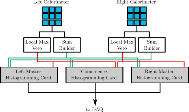
A schematic of the SyMB readout is shown in figure 6.2. For each calorimeter, the signals from each of the nine PMTs were summed in a sum-builder, and also sent to a logic unit called the local maximum veto. A veto signal was produced if any of the eight peripheral crystals had a larger signal than the central crystal. The purpose of this veto was to eliminate background which did not originate from the target. Particles from the target would pass through the collimator aperture and deposit the majority of their energy in the central crystal.

The sums and vetos were sent to three fast histogramming cards, called the left master, right master, and coincidence histogram cards. The left master required that the trigger conditions be met by the left calorimeter. The right master required that the trigger conditions be met by the right calorimeter. The coincidence card required a trigger from both calorimeters. Each card stored a two-dimensional histogram, in which one dimension represented the energy sum from the left calorimeter, and the other dimension represented the energy sum from the right calorimeter.

The calorimeters were subject to high rates, on the order of tens of kilohertz, but were designed to operate without any dead-time. The amount of time needed to digitize and record the energy deposited from an electromagnetic shower was shorter than the DORIS bunch spacing (approximately 100 ns). That meant that the SyMBs could easily differentiate events in adjacent bunches. The bunch width in DORIS was less than 2 ns, so multiple interactions within the same bunch crossing of the target could not be distinguished at all. In such multi-interaction events, the calorimeters recorded a sum of the energy deposited from all of the interactions. Given these sort of time scales, the SyMB essentially measured the total energy deposited from each bunch crossing. Rather than measuring the number of events in a given amount of time, the SyMBs measured the number of bunch crossings in which an event of interest took place.

6.2.2 SyMB Data

The SyMB data came in the form of three two-dimensional histograms, one from each histogramming card. The high rates in the SyMBs would have swamped the OLYMPUS data acquisition system (DAQ), so rather than reading out every event, the DAQ would periodically (every 30,000 main triggers, approximately once per minute of wall-time) read out and reset the SyMB histograms. This meant that event-by-event information was not recorded. Instead, the SyMB histograms show the aggregation of the events over the period between readouts. The three histograms are shown in figures 6.3, 6.4, and 6.5, for a typical run. Each count in the histograms corresponds to one bunch crossing of the target.

Figure 6.3: The coincidence histogram was filled when the threshold and local-maximum conditions were satisfied by both calorimeters.

Figure 6.4: The right-master histogram was filled when the threshold and local-maximum conditions were satisfied by the right calorimeter.

Figure 6.5: The left-master histogram was filled when the threshold and local-maximum conditions were satisfied by the left calorimeter.

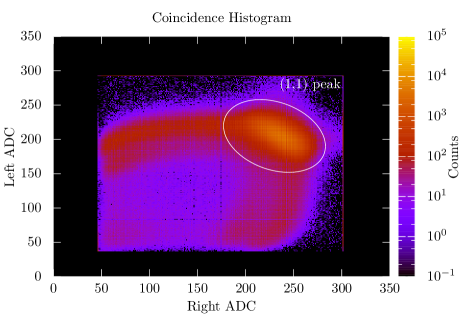
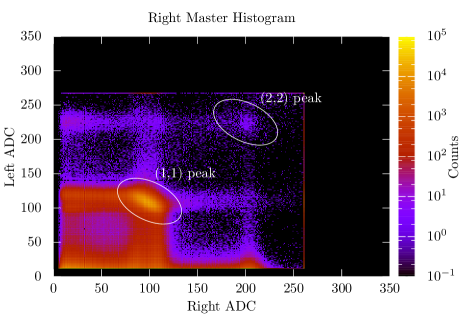
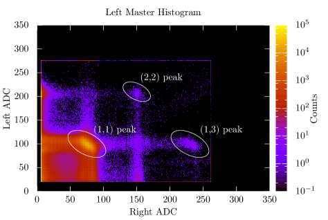
To good approximation, there were only two sorts of events which deposited energy in the SyMB calorimeters. The first was symmetric lepton-lepton scattering—Møller scattering ($e^{-}e^{-}\rightarrow e^{-}e^{-}$) during electron running and Bhabha scattering ($e^{+}e^{-}\rightarrow e^{+}e^{-}$) during positron running. In symmetric Møller/Bhabha scattering, approximately 1 GeV of energy was deposited in the left calorimeter and 1 GeV of energy was deposited in the right calorimeter. The second type of event was elastic lepton-proton scattering, in which the scattered lepton deposited 2 GeV of energy in one of the calorimeters. Neglecting cases where leptons lost energy from scattering in the lead collimator before entering the calorimeter, the calorimeters saw integer numbers of GeV at each bunch crossing. Since multiple interactions could occur within one bunch crossing, this number could sometimes exceed the beam energy (2 GeV). In this thesis, I will refer to the various signal peaks using a two-dimensional coordinate system where the first coordinate refers to the number of GeV deposited in the left calorimeter, and the second coordinate refers to the number of GeV deposited in the right calorimeter. For example, if 1 GeV were deposited in the left calorimeter, and 3 GeV were deposited in the right, this event would fall in the (1,3) signal peak. The probability of any events occuring in a single bunch was low, so the likeliest energy deposition in any given bunch was (0,0).

The three histograms had different dynamics ranges, so not all of the histograms had all of the same signal peaks. Furthermore, not all of the peaks had count-rates close to what was expected from simulation. The cause of these discrepant count-rates was not conclusively determined, although we formulated a hypothesis that is consistent with the observed discrepancies [101]. I will summarize here the different peaks that are present in the three histograms, the problems with each, and the explain the specific combination of count-rates which can produce a useful luminosity extraction.

The histograms did have underflow and overflow bins for events in which the energy was outside of the histogram’s dynamic range. In principle, the information in these bins could have been used to extract luminosity information. For example, the (2,0) peak in the left master histogram could have been used to extract the rate of elastic $ep$ scattering. In practice, the rates of the underflow and overflow bins were anomalous—in some cases too high and in other cases too low compared to simulation—and we came to conclusion that these bins did not function properly. In the interest of brevity, I will not cover the underflow and overflow signal peaks in this section.

Coincidence Histogram

The coincidence histogram, shown in figure 6.3, had the smallest dynamic range of the three histograms, in both the left and right axes. Only the (1,1) signal peak was visible below the overflow. In the main SyMB analysis, luminosity was extracted by comparing the number of counts in the (1,1) signal peak to simulation. In doing so, we found that the ratio $\mathcal{L}_{e^{+}p}/\mathcal{L}_{e^{-}p}$ is 5% smaller than that of the slow control system and the $12^{\circ}$ telescopes during the latter part of the fall run. (The discrepancy varies from 2% to 5% depending on which part of the fall run is considered.) This discrepancy, as well as the large systematic uncertainties from the method itself, prevent us from trusting the main SyMB analysis.

Right Master Histogram

In the right master histogram, shown in figure 6.4, the dynamic range was slightly wider so that both the (1,1) and (2,2) signal peaks were visible. The (1,1) peak had a similar rate to the (1,1) peak in the coincidence histogram, i.e., it had the same species-dependent discrepancy.

The (2,2) peak was populated by two different classes of multi-interaction events. In the first class, there are two symmetric Møller/Bhabha interactions in the same bunch crossing. Two leptons hit the left calorimeter, and two hit the right calorimeter. In the second class, there are two $ep$ elastic events in which the leptons hit opposite calorimeters. By using the simulated rates of $ee$ and $ep$ scattering, we estimated how how many (2,2) counts we should expect. We found that the right master histogram has only 50–60% of the expected rate, and therefore cannot be used for a trustworthy luminosity measurement.

The right master histogram had a lattice-like structure caused by coincidence events in which one particle lost some energy (say, in the collimator) before entering the calorimeter. There were cross-like structures at (1,2) and (2,1), where lattice lines intersected. Events falling at these positions were multi-interaction events in which one event was a Møller/Bhabha interaction with only one lepton entering a calorimeter. The SyMB apertures had a large degree of overlap; that is, if one lepton passed through the left aperture, the chances were good that the other lepton would make it through the right aperture. The consequence was that the (1,2) and (2,1) peaks were not very clearly defined and were not readily useable for analysis.

Left Master Histogram

The left master histogram, shown in figure 6.5, included, in addition to the (1,1) and (2,2) peaks, a third signal peak at (1,3). Events in this peak were produced by a symmetric Møller/Bhabha interaction occuring in the same bunch as an $ep$ scattering in which the lepton entered the right calorimeter. The Møller/Bhabha interaction put 1 GeV in both calorimeters, while the $ep$ lepton deposited an additional 2 GeV in the right calorimeter.

The (1,1) rate matched what is observed in both the right master and coincidence histograms; it had the same species-dependent discrepancy when compared with slow control and the $12^{\circ}$-system. The (2,2) rate was slightly lower than that of the right master histogram. The peak had about 40% of the counts one would expect given the simulated $ep$ and $ee$ rates.

The rate in the (1,3) peak was very close to what would be predicted from the Møller/Bhabha and $ep$ cross sections. In a given run period, the number of (1,3) events should, to lowest order, follow the relation:

$$N_{(1,3)}=\frac{\mathcal{L}^{2}\sigma_{(1,1)}\sigma_{ep\rightarrow R}}{N_{b}}=\frac{\mathcal{L}N_{(1,1)}\sigma_{ep\rightarrow R}}{N_{b}}$$ (6.1)

where $N_{b}$ is the number of bunch crossings and $\mathcal{L}$ is the integrated luminosity during the run period. For the sake of simplicity, we can estimate $\mathcal{L}$ using the slow control system. If one uses simulation to estimate $\sigma_{(1,1)}$ and $\sigma_{ep\rightarrow R}$, then the ratio of (1,3) data rate to prediction shows a slight beam-species dependence, which is strikingly similar to the beam-species dependence of the Møller/Bhabha luminosity extraction. If, instead, one estimates $\sigma_{(1,1)}$ directly from the (1,1) peak in data, then the ratio of data to prediction in the (1,3) peak has practically no apparent beam-species dependence.

It seemed that whatever was causing the beam-species dependence in the main Møller/Bhabha luminosity extraction, caused the same beam-species dependence in the (1,3) rate. That meant that the (1,3) and (1,1) peaks together could be used to extract a reasonable estimate of luminosity.

6.3 Multi-Interaction Event Analysis

To extract a luminosity from the Left Master (1,1) and (1,3) peaks, we need to make a few assumptions about the cause of the problems in the main SyMB analysis. To summarize the main problem, the rate of Møller events in data is about 5% too low (relative to expectation from simulation and slow control) whereas the rate of Bhabha events in data is not. That is:

$$\frac{N^{\text{data}}_{e^{-}e^{-}}}{\sigma^{\text{sim.}}_{e^{-}e^{-}}\times\mathcal{L}^{\text{s.c.}}_{e^{-}e^{-}}}\times\frac{\sigma^{\text{sim.}}_{e^{+}e^{-}}\times\mathcal{L}^{\text{s.c.}}_{e^{+}e^{-}}}{N^{\text{data}}_{e^{+}e^{-}}}\approx 0.95.$$ (6.2)

We assume that there are two possible ways for this discrepancy to occur. One possibility is that the Møller/Bhabha simulation may be inaccurate in a way that over-predicts the Møller cross section, i.e., $\sigma^{\text{sim.}}_{e^{-}e^{-}}$ is too large. The other possibility is that the calorimeters or their DAQ system may have some sort of inefficiency during electron-beam running, i.e., $N^{\text{data}}_{e^{-}e^{-}}$ is too low. We would like that our luminosity extraction be robust to both of these causes. We should avoid using $\sigma^{\text{sim.}}_{e^{\pm}e^{-}}$, and any use of $N^{\text{data}}_{e^{\pm}e^{-}}$ should be made relative to $N^{\text{data}}_{(1,3)}$ so that any effective inefficiency will cancel.

6.3.1 Derivation

In a bunch crossing, there is a large number of beam particles, but the probability of any one beam particle having an $ee$ or $ep$ interaction is small. Therefore, we can use the Poisson distribution to describe the number of interactions in a bunch crossing. Specifically, the probability of having $N$ interactions in a bunch with integrated luminosity $\mathcal{L}_{j}$ is given by:

$$P(N)=\frac{e^{-\sigma\mathcal{L}_{j}}(\sigma\mathcal{L}_{j})^{N}}{N!}$$ (6.3)

where $\sigma$ is the cross section for an interaction.

Let us classify three types of interactions which can put energy into the SyMBs. Møller/Bhabha interactions, denoted by $ee$, put 1 GeV in each calorimeter. An $ep$ interaction where the lepton deposits 2 GeV of energy in the left calorimeter will be denoted by $ep\rightarrow L$. And $ep$ interactions where the lepton deposits 2 GeV of energy in the right calorimeter will be denoted by $ep\rightarrow R$.

The probability for a bunch crossing to result in energy deposition of the form (1,1) is given by:

$$P(1,1)= P_{ee}(1)\times P_{ep\rightarrow L}(0)\times P_{ep\rightarrow R}(0)$$ (6.4)

$$= e^{-\mathcal{L}_{j}(\sigma_{ee}+\sigma_{ep\rightarrow L}+\sigma_{ep\rightarrow R})}\times\sigma_{ee}\mathcal{L}_{j}$$ (6.5)

$$= e^{-\mathcal{L}_{j}\sigma_{\text{tot.}}}\times\sigma_{ee}\mathcal{L}_{j}.$$ (6.6)

In the same way, we can define the probability for energy deposition of the form (1,3):

$$P(1,3)= P_{ee}(1)\times P_{ep\rightarrow L}(0)\times P_{ep\rightarrow R}(1)$$ (6.7)

$$= e^{-\mathcal{L}_{j}(\sigma_{ee}+\sigma_{ep\rightarrow L}+\sigma_{ep\rightarrow R})}\times\sigma_{ee}\sigma_{ep\rightarrow R}\mathcal{L}_{j}^{2}$$ (6.8)

$$= e^{-\mathcal{L}_{j}\sigma_{\text{tot.}}}\times\sigma_{ee}\sigma_{ep\rightarrow R}\mathcal{L}_{j}^{2}.$$ (6.9)

To find the number of counts in a given peak from a given run period, we must sum these probabilities over the number of bunches in the run. If the total number of bunches in a run period is $N_{b}$, and the total integrated luminosity for the run period $\mathcal{L}$ is given by $\mathcal{L}=\sum_{j}^{N_{b}}\mathcal{L}_{j}$, then we find, in the large $N_{b}$ limit, that:

$$N_{(1,1)}= \sum\limits_{j=0}^{N_{b}}P(1,1)=\sum\limits_{j=0}^{N_{b}}\left[e^{-\mathcal{L}_{j}\sigma_{\text{tot.}}}\times\sigma_{ee}\mathcal{L}_{j}\right]$$ (6.10)

$$N_{(1,3)}= \sum\limits_{j=0}^{N_{b}}P(1,3)=\sum\limits_{j=0}^{N_{b}}\left[e^{-\mathcal{L}_{j}\sigma_{\text{tot.}}}\times\sigma_{ee}\sigma_{ep\rightarrow R}\mathcal{L}_{j}^{2}\right].$$ (6.11)

For the cross sections and bunch luminosities we are dealing with, $\mathcal{L}_{j}\sigma_{\text{tot.}}\ll 1$. It makes sense to recast the exponentials as series in powers of $\mathcal{L}_{j}\sigma_{\text{tot.}}$, which can be truncated. Now, dividing the two rates, and dropping any terms beyond first order in $\mathcal{L}_{j}\sigma_{\text{tot.}}$, we get:

$$\frac{N_{(1,3)}}{N_{(1,1)}} =\frac{\sigma_{ep\rightarrow R}\sum\limits_{j=0}^{N_{b}}\mathcal{L}_{j}^{2}\left[1-\mathcal{L}_{j}\sigma_{\text{tot.}}\right]}{\sum\limits_{j=0}^{N_{b}}\mathcal{L}_{j}\left[1-\mathcal{L}_{j}\sigma_{\text{tot.}}\right]}$$ (6.12)

$$=\frac{\sigma_{ep\rightarrow R}N_{b}\left[\langle\mathcal{L}_{j}^{2}\rangle-\sigma_{\text{tot.}}\langle\mathcal{L}_{j}^{3}\rangle\right]}{\left[\mathcal{L}-N_{b}\sigma_{\text{tot.}}\langle\mathcal{L}_{j}^{2}\rangle\right]}$$ (6.13)

$$=\frac{\sigma_{ep\rightarrow R}N_{b}}{\mathcal{L}}\left[\langle\mathcal{L}_{j}^{2}\rangle-\sigma_{\text{tot.}}\langle\mathcal{L}_{j}^{3}\rangle\middle]\middle[1+\frac{N_{b}}{\mathcal{L}}\sigma_{\text{tot.}}\langle\mathcal{L}_{j}^{2}\rangle\right].$$ (6.14)

From here, we can use the relation that the variance in luminosity per bunch, $v_{b}$, is equal to $\langle\mathcal{L}_{j}^{2}\rangle-\langle\mathcal{L}_{j}\rangle^{2}$, or equivalently $\langle\mathcal{L}_{j}^{2}\rangle-\mathcal{L}^{2}/N_{b}^{2}$. We’ll proceed with some rearranging, and drop the $\sigma_{\text{tot.}}^{2}$ term:

$$\frac{N_{(1,3)}}{N_{b}N_{(1,1)}\sigma_{ep\rightarrow R}} =\frac{1}{\mathcal{L}}\left[\left(v_{b}+\frac{\mathcal{L}^{2}}{N_{b}^{2}}\right)-\sigma_{\text{tot.}}\langle\mathcal{L}_{j}^{3}\rangle\middle]\middle[1+\frac{N_{b}}{\mathcal{L}}\sigma_{\text{tot.}}\left(v_{b}+\frac{\mathcal{L}^{2}}{N_{b}^{2}}\right)\right]$$ (6.15)

$$=\frac{\mathcal{L}}{N_{b}^{2}}+\frac{v_{b}}{\mathcal{L}}+\frac{N_{b}\sigma_{\text{tot.}}}{\mathcal{L}^{2}}\left\{\left(v_{b}+\frac{\mathcal{L}^{2}}{N_{b}^{2}}\right)^{2}-\frac{\langle\mathcal{L}_{j}^{3}\rangle\mathcal{L}}{N_{b}}\right\}.$$ (6.16)

We can rearrange this to get an expression for luminosity:

$$\mathcal{L}=\frac{N_{(1,3)}N_{b}}{N_{(1,1)}\sigma_{ep\rightarrow R}}-\frac{v_{b}N_{b}^{2}}{\mathcal{L}}-N_{b}\sigma_{\text{tot.}}\left\{\left(\frac{v_{b}N_{b}}{\mathcal{L}}+\frac{\mathcal{L}}{N_{b}}\right)^{2}-\frac{\langle\mathcal{L}_{j}^{3}\rangle N_{b}}{\mathcal{L}}\right\}.$$ (6.17)

Equation 6.17 shows that luminosity can be estimated from a main term, $N_{(1,3)}N_{b}/N_{(1,1)}\sigma_{ep\rightarrow R}$, with some corrections. In this derivation, I only kept terms to first order in $\mathcal{L}\sigma_{\text{tot.}}$, but, if necessary, corrections can be calculated to arbitrary order.

Let us consider the meaning of these corrections. The first correction term, $v_{b}N_{b}^{2}/\mathcal{L}^{2}$, describes the effect of luminosity variance between bunches. High-luminosity bunches are much more likely to have multi-interaction events than low-luminosity bunches. If there is variance between the bunches, this will have a small effect on the multi-interaction event rate. The second correction term, which has a leading factor of $\sigma_{\text{tot.}}$, accounts for the fact that there may be three interactions in a bunch crossing. Some small fraction of would-be (1,3) events will fall outside of the (1,3) peak because of additional energy deposited by a third interaction in the same bunch.

Figure 6.6: Bunch luminosity variance is a percent-level correction. Higher order multi-interactions matter at the per-mil level. This justifies neglecting subsequent terms in the $\mathcal{L}\sigma_{\text{tot.}}$ expansion.

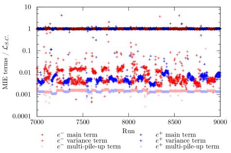
Figure 6.6 shows the scale for these correction terms relative to the luminosity estimate from slow control $\mathcal{L}_{S.C.}$. The variance term is highly species-dependent, and corrects the luminosity extraction by a few percent. This term is absolutely necessary to achieve percent-level accuracy desired for OLYMPUS. The correction for higher order multi-interaction events is smaller, on the order of one to two tenths of a percent. It stands to reason that subsequent higher-order terms will be even smaller and will not be significant for a percent-level luminosity estimate. This justifies the decision to truncate our power expansion at first order.

The result in equation 6.17 shows the relationship between fundamental quantities like cross sections, count rates, and luminosities. To apply this relation to a useable luminosity extraction, we must decide how to estimate these fundamental quantities, consistent with the assumptions laid out at the beginning of this section. Let us first look at the quantites in the main term. $N_{(1,3)}$ and $N_{(1,1)}$ naturally come from data; we must integrate the left master histogram around the signal peaks. $N_{b}$ is known to good accuracy from the slow control live-time and the DORIS average bunch spacing (96.8 ns). In principle, $\sigma_{ep\rightarrow R}$ could be estimated from data, but since this signal shows up in the unreliable histogram underflow, we cannot trust it. Instead, we can estimate this using simulation.

I want to point out that equation 6.17 isn’t the result of solving for $\mathcal{L}$. In fact, $\mathcal{L}$ appears on both sides of the equation. However, $\mathcal{L}$ has been eliminated from the main term. In the correction terms, we can estimate $\mathcal{L}$ from the slow control system. Any slight deviations from the real luminosity will have a negligible effect on already small corrections.

The bunch luminosity variance, $v_{b}$, as well as $\langle\mathcal{L}_{j}^{3}\rangle$ require some work to estimate. Both depend on the variation of current within the 10 bunches of DORIS, as well as the variation in time of those currents. To estimate these, I use a readout from the DORIS computer which shows the individual bunch currents as a function of time. I then use the OLYMPUS slow control system to estimate the target density so that I can reconstruct the individual bunch luminosities.

The last remaining quantity is $\sigma_{\text{tot.}}$, which has the components $\sigma_{ep\rightarrow L}$, $\sigma_{ep\rightarrow R}$, and $\sigma_{ee}$. The $ep$ cross sections must come from simulation as discussed earlier. $\sigma_{ee}$ can be estimated using either simulation or from the (1,1) peak in data. Because the higher-order multi-interaction term is so small, the difference between using simulation or data to estimate $\sigma_{ee}$ is negligible. Putting this all together, our estimate of the luminosity becomes:

$$\mathcal{L}=\frac{N_{(1,3)}^{\text{data}}N_{b}}{N_{(1,1)}^{\text{data}}\sigma_{ep\rightarrow R}^{\text{sim.}}}-\frac{v_{b}N_{b}^{2}}{\mathcal{L}_{S.C.}}-N_{b}\sigma_{\text{tot.}}^{\text{sim.}}\left\{\left(\frac{v_{b}N_{b}}{\mathcal{L}_{S.C.}}+\frac{\mathcal{L}_{S.C.}}{N_{b}}\right)^{2}-\frac{\langle\mathcal{L}_{j}^{3}\rangle N_{b}}{\mathcal{L}_{S.C.}}\right\}.$$ (6.18)

6.3.2 Analysis Procedure

Extracting a count rate from a signal peak in a histogram requires integrating over the peak between some bounds. The placement of the bounds obviously affects the result of the integral, and this is problematic. The best solution to this problem is to simulate every histogram as a reference, and to integrate the data histogram and simulation histogram over the same bounds. That avenue isn’t available to us because we want to avoid using the Møller/Bhabha simulation.

At the same time, the lack of a reference simulation is freeing. We will have to place arbitrary bounds, so we can do so without too much angst. At the end, we must test that our choice of bounds has a minimal effect on our extraction of the species-relative luminosity, even if that choice has a large effect on the various integrals. For this reason, in my analysis I have chosen to make simple box cuts, centered around the various signal peaks.

Figure 6.7: I fit the one-dimensional ADC spectrum to find the peak positions.

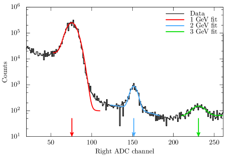
To ascertain the centroids of the signal peaks, I fit the 1-dimensional ADC spectra with a signal-plus-background model:

$$f(x|A,\mu,\sigma,B,\tau,C)=Ae^{-\frac{(x-\mu)^{2}}{2\sigma^{2}}}+\frac{B}{1+e^{\frac{x-\mu}{\tau}}}+C.$$ (6.19)

I take the parameter $\mu$ to be the peak position. I do this for the 1 and 2 GeV peaks in the left ADC spectrum and the 1, 2, and 3 GeV signal peaks in the right ADC spectrum, as shown in figure 6.7.

Figure 6.8: The signal peak positions changed slightly over the fall run. The 3 GeV peak in the right ADC is very close to the over-flow level, especially early on. If the box cut size is too large, the box will run off the end of the histogram, throwing off the luminosity determination. The solution is to use tighter boxes for the earlier runs. Additionally, one can see that when using the negative toroid polarity, the performance of the SyMB’s PMTs was altered enough to noticeably shift the peak positions downward.

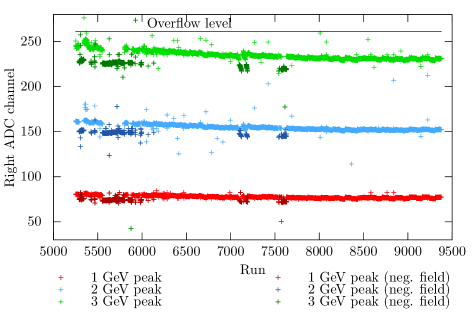
Figure 6.8 shows how the peak positions for the right ADC (in the left master histogram) evolve over the course of the fall run. The peak positions shift over time to lower channel numbers. In the early part of the run, the 3 GeV peak is quite close to the overflow boundary. To avoid clipping, any studies involving these runs need quite tight boxes.

Since all three peak positions change, it makes sense to set the box width based on a fixed energy scale, rather than a fixed number of ADC channels. The ADC spectra must then be calibrated to develop a conversion between units of energy and ADC channels. For the results I show in this note, I used a linear calibration for the left master’s left ADC (using the 1 and 2 GeV peak positions), and a quadratic calibration for the right ADC (using the 1, 2, and 3 GeV peak positions). I integrated over a fixed window with a half-width of 286 MeV for both the left and right ADCs. The cross sections $\sigma_{ep\rightarrow L}$ and $\sigma_{ep\rightarrow R}$ were found by integrating the simulated histograms over bins [200,250] and [185,230] respectively.

6.4 Systematic Uncertainties

The accuracy of the MIE luminosity determination is limited by a handful of systematic effects. Slight inaccuracy in the beam position, the detector geometry, the magnetic field, or of the energy of the beam in simulation can produce slight inaccuracy in the calculation of $\sigma_{ep}$. The box cut procedure can affect the results of $N_{(1,3)}$ and $N_{(1,1)}$. The specific radiative corrections procedure used in simulation can change the definition of $\sigma_{ep}$. In this section, I will go through each of these and estimate their effect on the MIE determination of the species relative luminosity.

The numbers I will present in this section are the percent uncertainties in the determination of the species relative luminosity, which I define as $\mathcal{L}_{e^{+}p}/\mathcal{L}_{e^{-}p}$. The uncertainty in this quantity, which I’ll call $\delta_{\mathcal{R}}$, produces a uniform baseline uncertainty for all of the asymmetry measurement points, in the form: $\delta_{A}\approx\delta_{R}/2$. That is, a two percent uncertainty in the relative luminosity produces a one percent uncertainty in the asymmetry in every bin.

Whereas, in the main SyMB analysis the systematic uncertainties proved to be so large to make the analysis unusable, the MIE result is much more robust with respect to systematic uncertainties. I estimate the systematic uncertainty on the species-relative luminosity to be 0.27%. A breakdown of the various systematics is shown in table 6.1.

Systematic	Value (%)
Beam Position	0.21
Geometry	0.13
Box Sizes	0.10
Magnetic Field	0.05
Radiative Corrections	0.03
Beam Energy	0.01
Total	0.27

Table 6.1: I estimate the systematic uncertainy of the multi-interaction event species-dependence to be 0.27%, making this system viable for the OLYMPUS analysis.

6.4.1 Beam Position

Figure 6.9: The cross section $\sigma_{ep\rightarrow R}$ is unaffected by changes in the beam’s vertical position, but changes in the horizontal position have a 5.7%/mm effect, which is independent of beam species.

Figure 6.10: The cross section $\sigma_{ep\rightarrow R}$ is unaffected by changes in the beam’s vertical slope, but changes in the horizontal slope have a 17%/mrad effect, which is nearly independent of beam species.

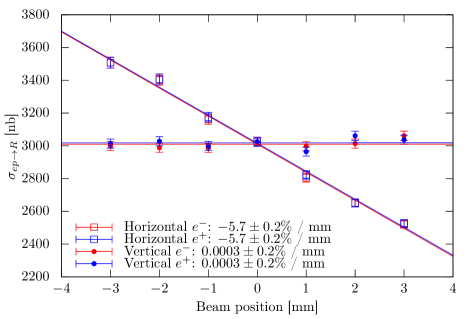
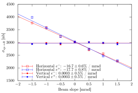
If there were an inaccuracy in our knowledge of the beam position, this would lead us to calculate an erroneous value of $\sigma_{ep\rightarrow R}^{\text{sim.}}$. We would be simulating the beam in one position, when in reality it occupied another. We can estimate the effect by altering the beam position in simulation and looking at the change $\sigma_{ep\rightarrow R}^{\text{sim.}}$. Figures 6.9 and 6.10 show the results of simulations with varying beam position offsets and slopes. Generally, the cross section $\sigma_{ep\rightarrow R}^{\text{sim.}}$ is unaffected by changes in the beam’s vertical parameters, but has a large dependence on the beam’s horizontal parameters. This dependence essentially doesn’t change with beam species. However there are ways that a species-dependent systematic might manifest itself.

Figure 6.11: The electron beam tended to sit about 400 $\mu$m to the left of the positron beam at both BPMs. While upstream the two beams had roughly the same vertical position, this grew to about 300 $\mu$m by the downstream BPM.

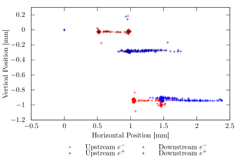
Let us consider two ways in which a species-dependent systematic might occur:

1. The survey of the BPM positions inaccurately captures the true BPM axes, such that the true axes are rotated from the supposed axes. Since the two species have slightly different vertical beam positions (shown in figure 6.11), this error would introduce an additional species-dependent horizontal offset for which we do not account.

2. The BPMs themselves have some species-dependent inaccuracy.

In the following section, I will present our estimates for the accuracy of the BPMs. Following that I will calculate the magnitude of the two sources of species-dependent systematic effects.

Accuracy of the BPMs

The accuracy of the beam position in simulation is determined by two factors:

• The accuracy of the survey of the beam position monitors (Were the BPMs physically located where we believed them to be?)

• The accuracy of the BPM readout calibration (Are we interpreting the BPM data correctly?)

Let’s address these in turn.

The accuracy of the BPM survey has a species-independent effect on the simulation. We can estimate the survey accuracy by looking at the residuals of the fits to survey data. The residuals indicate that the BPMs are constrained in position to 200 $\mu$m. However, the orientation of the BPM axes are not as well constrained. During the survey, a target ball was moved along the four cap faces of each monitor to establish the planes of the caps in order to fix the orientation of the monitor axes. For one of the BPMs, these survey points are only coplanar on the level of 500 $\mu$m accuracy. Therefore, we estimate the relative orientation of the axes of the two monitors is good to within a rotation of 500 $\mu$m over a 55 mm radius, or approximately $0.52^{\circ}$.

The accuracy of the BPM readout is much better than 200 $\mu$m, so the species-independent part of this effect can be safely neglected in comparison to the BPM survey. The crucial number is thus the species-dependent readout accuracy. For the majority of later runs, the Libera readout was available. The Libera readout produces a position measurement that is independent of the current direction, and therefore species independent to a high degree. Looking at the non-linearity of the fits to the calibration data, and by attributing all of that to a possible species-dependent effect, we estimate that the BPMs have a species-dependent accuracy of 20 $\mu$m. We believe that the majority of any species-dependent inaccuracy (caused by the effect of the beam profile, or caused by the choice of functional form used to fit the calibration data) will be correlated between the BPM modules. Uncorrelated species-dependent inaccuracy could also be problematic, as it can introduce changes in measured beam slope bewteen the two species. Therefore, we conservatively estimate a limit of 10 $\mu$m for any uncorrelated, species-dependent inaccuracies of the BPM calibration.

BPM Axis Rotation

In subsubsection 6.4.1, I estimated the accuracy of the relative orientation of the BPM axes to be 0.52^∘. As seen in figure 6.11, the two species have a slightly different vertical position and slope. At the center of the target, the two beams are vertically offset by about 140 $\mu$m. The systematic uncertainty from an introduced horizontal offset is:

$$\delta_{\text{rot. pos.}}=140\mu\text{m}\times\sin\left(0.52^{\circ}\right)\times\frac{5.7\%}{\text{mm}}=0.007\%.$$

A rotation of the BPM axis could also introduce an artificial horizontal slope. The measured difference in vertical slopes between the two species is on the order of 300 $\mu$m over the 1.464 m between the two BPMs. The systematic uncertainty is:

$$\delta_{\text{rot. slo.}}=\frac{300\mu\text{m}}{1.464~{}\text{m}}\times\sin\left(0.52^{\circ}\right)\times\frac{17.7\%}{\text{mrad}}=0.03\%.$$

Species-Dependent BPM Inaccuracy

In subsubsection 6.4.1, I estimated that the BPMs have a 20 $\mu$m species-dependent uncertainty that is fully correlated between the two monitors, and a 10 $\mu$m species-dependent uncertainty that is uncorrelated between the two monitors. The uncertainty from an introduced position offset would be:

$$\delta_{\text{corr. pos.}}=20\mu\text{m}\times 5.7\%/\text{mm}=0.11\%$$

from the correlated uncertainty, and:

$$\delta_{\text{pos.}}=10\mu\text{m}\times\frac{\sqrt{z_{1}^{2}+z_{2}^{2}}}{(z_{1}+z_{2})^{2}}\times 5.7\%/\text{mm}=0.04\%$$

from the uncorrelated uncertainty, where $z_{1}=-0.801$ m and $z_{2}=0.663$ m are the positions of the two beam position monitors. The uncertainty from an introduced slope (produced only by the BPM’s uncorrelated uncertainty) would be:

$$\delta_{\text{slo.}}=\frac{10\mu\text{m}\sqrt{2}}{1.464\text{m}}\times 17.7\%/\text{mm}=0.17\%.$$

Totals

We can combine these uncertainties to get a total uncertainty from the BPMs.

$$\delta_{\text{BPM}}=\sqrt{\delta_{\text{rot. pos.}}^{2}+\delta_{\text{rot. slo.}}^{2}+\delta_{\text{corr. pos.}}^{2}+\delta_{\text{pos.}}^{2}+\delta_{\text{slo.}}^{2}}=0.21\%$$

Remark on the Neumann Readout

Between runs 7357 and 7358, the Libera BPM readout was connected. Prior to run 7358, only the Neumann readout was available. However, only the Libera readout was used for the BPM calibration. Generally, we trust the Libera readout more than the Neumann since its calibration is beam species independent. Up until now, I have limited my discussion to analysis of runs in which the Libera readout was available. At some point, it may become valuable to extract luminosities from the earlier Neumann runs. I have studied the differences between the two systems over the runs that they overlap and I believe the change in readout contributes negligibly to the accuracy of the analysis.

To simulate runs prior to 7358, a few intermediate steps are needed to estimate the beam position. By looking at the data from later runs when both readouts are present, we fit a map between the Libera and Neumann data. This map is species dependent. When simulating and early run, the map is first applied to the Neumann data to produce fake Libera data. These data are then analyzed using the BPM survey fits.

I tried to study the effect of not having Libera readout by looking at the later runs. I looked at the difference in the beam position reconstructed from Libera data to the beam position reconstructed from the Neumann data (through the intermediate steps). The differences in position are on the order 1 $\mu$m, and the differences in slope are on the order of 1 $\mu$rad. Even if these differences were maximally species dependent, they would be insignificant compared to the those from $\delta_{\text{BPM}}$. Therefore I think there is no need to worry about using the early data.

6.4.2 Geometry

If the SyMB detectors sit in a slightly different place in simulation compared to reality, this might distort our calculation of $\sigma_{ep\rightarrow R}^{\text{sim.}}$. To estimate this effect, I ran simulations with the SyMBs in slightly different positions to see how this might affect the cross section, specifically looking at species dependence. The results are shown in figures 6.12 and 6.13.

Figure 6.12: Moving the right SyMB 1 mm in $x$ produces a 0.13% change in the species ratio. Moving the right SyMB in $y$ produces no significant effect.

Figure 6.13: Rotating the right SyMB 1^∘ about the $x$-axis produces a 0.27% change in the species ratio. Rotating the right SyMB 1^∘ about the $y$-axis produces a 0.4% change in the species ratio.

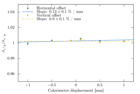
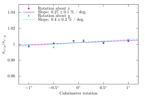
We estimate that the survey of the SyMBs was accurate to within 500 $\mu$m in position and to within 0.2^∘ in rotation. Therefore, we estimate the systematic errors to be:

$$\delta_{x\text{~{}pos.}}=500\mu\text{m}\times\frac{0.13\%}{\text{mm}}=0.07\%,$$

$$\delta_{x\text{~{}rot.}}=0.2^{\circ}\times\frac{0.27\%}{\text{deg.}}=0.05\%,$$

$$\delta_{y\text{~{}rot.}}=0.2^{\circ}\times\frac{0.40\%}{\text{deg.}}=0.08\%.$$

The systematic uncertainty from the $y$ position is harder to estimate because the result of the simulation shows zero effect, within the precision of the study. In this case, we can conservatively assume that the size of the effect is at most equal to the fit uncertainty:

$$\delta_{y\text{~{}pos.}}=500\mu\text{m}\times\frac{0.10\%}{\text{mm}}=0.05\%.$$

Combining these systematics, we get:

$$\delta_{\text{geom.}}=\sqrt{\delta_{x\text{~{}pos.}}^{2}+\delta_{y\text{~{}pos.}}^{2}+\delta_{x\text{~{}rot.}}^{2}+\delta_{y\text{~{}rot.}}^{2}}=0.13\%.$$

6.4.3 Box-Cut Procedure

As mentioned in section 6.3.2, care must be taken that the choice of cuts does not influence the result. To study this, I produced a species ratio for many different box cut sizes to look for any trends. The results are shown in figure 6.14. Fortunately, even large changes in the box cut size have a minimal impact on the luminosity species ratio. To estimate a systematic uncertainty, I calculated the standard deviation of the ratios for all of the different box sizes I tested: 0.10%.

Figure 6.14: Changing the box cut size does not have a significant impact on the luminosity species ratio.

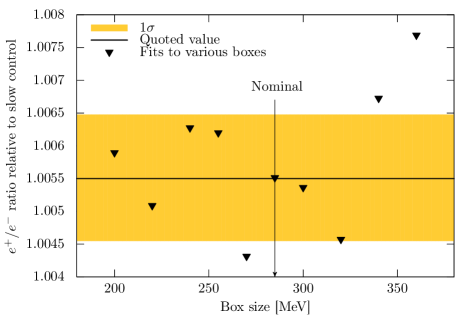
6.4.4 Magnetic Field

The magnetic field can have systematic offsets stemming from a variety of sources. The field may have a different value than what was measured. The position of the measurement point may be different than what was recorded. The interpolation procedure may introduce some residual error. All of these can contribute to distorting our calculation of $\sigma_{ep\rightarrow R}^{\text{sim.}}$.

As a first step, I calculated $\sigma_{ep\rightarrow R}^{\text{sim.}}$ for both beam species over a range of magnetic currents. This can give us a sense of the full scale of the effect of the magnetic field. The results, shown in figure 6.15, indicate that the field raises the $e^{-}p$ cross section and decreases $e^{+}p$ cross section, changing the species ratio by 0.53%. The magnitude of this effect does not indicate any sort of systematic error; if the field map is correct then this effect is accounted for in simulation. Rather, we need to judge if there could be any error in our understanding of this effect.

Figure 6.15: The magnetic field has the effect of raising the $e^{-}p$ cross section in the right SyMB while decreasing the $e^{+}p$ cross section. The cross sections are slightly different at zero current because of radiative effects.

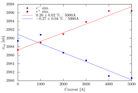
Ideally, we could use a data-driven method to test the slopes in figure 6.15 and assign a systematic uncertainty. I looked at several possibilities, but unfortunately none were successful. One way to judge the accuracy of the magnetic field would be to look at the size of residuals between the field map and the magnetic field survey data. However, the magnetic field map in the beamline region (the only region relevant for the SyMBs) is estimated by directly interpolating the field survey data points. Consequently we have no residuals to use. Another possibility is to look at the runs with different current settings to see if a slope can be extrapolated. Looking at the (0,2) peak counts did not yield anything useful because of problems with the histogram underflow bins. I also looked at the ratio of (1,3) to (1,1) peaks with the assumption that the slow control luminosity is accurate, but there are not enough runs with differing magnet currents and the statistics are poor.

Without a data driven approach to testing the slopes in figure 6.15 I will resort to arguments of scale. Conservatively, I have a high degree of confidence that our magnetic field is accurate to within 10%. Since the full effect of the magnetic field is to introduce a species difference of 0.5%, I estimate a systematic for the magnetic field to be 0.05%.

6.4.5 Radiative Corrections

The radiative $ep$ generator is used in the calculation of $\sigma_{ep\rightarrow R}^{\text{sim.}}$. There are several choices that can be made in calculating radiative corrections in which the options aren’t necessarily better or more accurate, but can still affect the results. Let’s consider a few of these:

• Form Factor Model – The form factors are used as an input to calculate proton vertex functions for all of the radiative diagrams, including bremsstrahlung. Ignoring hard two-photon exchange, which is not included in the OLYMPUS generator, the choice of form factor can influence the species ratio through the bremsstrahlung interference term.

• Hard vs. Soft Definition – Soft two-photon exchange must be included since its divergence is needed to cancel the divergence in lepton-proton bremsstrahlung interference. How one artificially defines the soft region of the two-photon contribution will affect the species ratio. Specifically, Maximon and Tjon define the soft region in a slightly different way than Mo and Tsai.

• Exponentiation vs. Non-exponentiation – Naively, radiative corrections involve the application of a factor $(1+\delta)$ to the one-photon cross section. The correction $\delta$, which is negative, accounts for next-to-leading order effects, and depends on the elastic cut-off. In the soft limit, one can account for radiative effects to all orders by substituting $(1+\delta)\longrightarrow\exp(\delta)$. Certainly exponentiation is more accurate for very small cut-off values. But it is not clear which method better reflects reality for large cut-offs.

Of these three choices, the only one that makes any detectable difference at the kinematics relevant to the SyMB is the choice of whether or not to exponentiate. Using the multiple weights in the OLYMPUS radiative $ep$ generator, I was able to reweight my simulation runs to see the effect of using exponentiation or not. The value of $\sigma_{ep\rightarrow R}^{\text{sim.}}$ is 0.05% higher when exponentiating.

To estimate a systematic uncertainty, I assumed that the difference between exponentiating represented the full width of our uncertainty about the true radiative correction, and that the quoted uncertainty should be half of that difference. I chose to round up to 0.03%.

6.4.6 Beam Energy

If the electron and positron beams have slightly different energies, then this will introduce a species difference to all of the cross sections involved. The change in Møller/Bhabha cross sections will cancel in the $N_{(1,3)}$ to $N_{(1,1)}$ ratio, but we do need to take into account the effect of the $ep$ cross section changing by species.

We estimate that the two beams were within 100 keV of energy of each other. The difference in the Rosenbluth cross sections at $1.27^{\circ}$, 100 keV apart in energy, is 0.01%, which I will quote as a systematic uncertainty.

6.5 Results

6.5.1 Time Dependence

Figure 6.16: The MIE and $12^{\circ}$ luminosity determinations have many of the same time-dependent variations when compared to the slow control system. That suggests that the slow control determination varied in time, probably due to temperature fluctuations in the target.

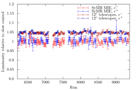
Figure 6.16 shows both the MIE luminosity determination and the $12^{\circ}$ tracking telescope luminosity determination relative to the luminosity determined by the slow control system, plotted over the set of runs used in the OLYMPUS analysis. The absolute luminosity is not determined by the MIE analysis (loosening or widening the box cuts changes the absolute luminosity determination) so the exact placement of the MIE points on the $y$ axis is arbitrary. The errorbars are statistical only, and one can see that the MIE analysis has a worse statistical precision than the $12^{\circ}$ system. The precision of the MIE analysis is largely limited by the statistics on $N_{(1,3)}$. Multi-interaction events happen more rarely than single-interaction events, so it comes as no surprise that the MIE method sacrifices precision. In this figure, each data point corresponds to ten runs aggregated together, to reduce the statistical errors per point.

The key result in figure 6.16 is that the MIE analysis and the $12^{\circ}$ systems see most of the same time-dependent variations when compared to the slow control system. This fact implicates the slow control system as being the source of most of the time-variation. This is probably caused by slight fluctuations in the target gas temperature, which are not entirely captured by the target cell temperature sensor. That the MIE analysis and $12^{\circ}$ analysis agree on many of the small scale time variations is a strong validation of both analyses.

6.5.2 Correction Factor to Slow Control

Figure 6.17: The MIE analysis suggests that the slow control luminosity for positrons is 0.55% too low relative to the slow control luminosity for electrons.

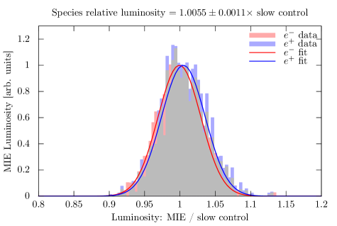
Since there are no major time-dependent trends in the MIE and slow control luminosity extractions, it is appropriate to use a luminosity correction factor to translate from the slow control luminosity (used by the OLYMPUS simulation) and the MIE luminosity, which we believe is more accurate. To determine this correction factor, the data in the top plot of figure 6.16 were projected onto the $y$ axis and histogrammed so that the distributions by species could be studied. The projections and gaussian fits are shown in figure 6.17. The distributions by species have slightly different means, indicating that the slow control luminosity has a slight species-dependent inaccuracy. The fits suggest that the slow control measures positron running luminosity to be 0.55% too low relative to electron running luminosity.

There is a statistical uncertainty on this correction factor of 0.11%. Despite the low statistics on $N_{(1,3)}$, when aggregating over many runs, the statistical uncertainty is still well below the systematic uncertainty of 0.27%. Adding these uncertainties in quadrature produces a total error on the species-relative luminosity of 0.29%. This meant that the OLYMPUS asymmetry measurements will have a global uncertainty of 0.15% (rounding up) due to luminosity.

6.5.3 Luminosity Normalization Point

Figure 6.18: Any physics result normalized to this analysis will take as an LNP: $\theta=1.27^{\circ}$, equivalent to $Q^{2}=0.002$ (GeV/$c$)², and $\epsilon=0.99975$.

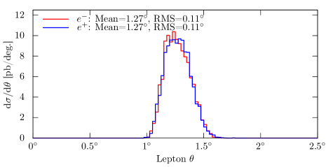
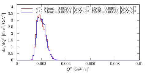
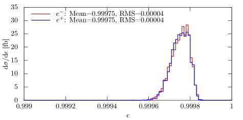
The multi-interaction event analysis depends on the elastic $ep$ cross section at the forward scattering angle of the right SyMB calorimeter (specifically, the collimator aperture). There is some contribution at that angle, however small, from hard two-photon exchange. Therefore, any result normalized to the MIE analysis will be relative to the lepton sign asymmetry at this angle. This angle is what is called a “Luminosity Normalization Point” (LNP).

To determine the precise location of the LNP, I looked at the generator output for simulated $ep$ events which entered the right calorimeter. The results are shown in figure 6.18. The LNP falls at a scattering angle of $1.27^{\circ}$, corresponding to a $Q^{2}$ of 0.002 (GeV/$c$)², and to value of $\epsilon$ equal to 0.99975. These values are very similar for both beam species.

6.6 Discussion

It was surprising to find that the MIE analysis, which was explored as an afterthought, had the smallest systematics of any of the OLYMPUS luminosity monitors. However, after comparing systematics with the main SyMB analysis, it became apparent that the MIE analysis had several inherent advantages. I will conclude this chapter by discussing these advantages, and discussing what improvements could be made if a luminosity monitor were designed around the MIE method.

6.6.1 Inherent Advantages of MIE

The single biggest advantage of the MIE method is that its luminosity extraction comes from the ratio of two count-rates, rather than a single countrate. Any pernicious systematics which affect electron running differently from positron running, must also affect both count rates differently. If the detectors have any inefficiency, or if the data acquisition system occasionally fails to add an event to the histogram, these effects will cancel in the ratio of count-rates. Clearly, some effect of this kind troubled the main SyMB analysis and produced a discrepancy in the species-relative luminosity. The MIE analysis was immune. There are examples of systematics which do affect the two count-rates differently: beam position and survey geometry come to mind. But these systematics largely affect the two beam species in the same way and the system is only barely sensitive to them when extracting a species relative luminosity.

Another advantage, which was in a way a happy accident, is that the two signal peaks were treated identically by the trigger. The (1,3) peak visible in data was only visible in the left master histogram (shown previously in figure 6.5). Only signals in the left calorimeter were considered in the trigger, and the (1,1) and (1,3) peaks have identical energy deposition on the left. One hypothesis for the cause of problems in the main analysis and of the deficits in the (2,2) peaks is inappropriate vetos [101]; the MIE analysis is completely immune to such problems.

Figure 6.19: The cross section for events in the SyMB calorimeters changes by almost a factor of two between electron running (red) and positron running (blue). This is not ideal when making a relative luminosity measurement.

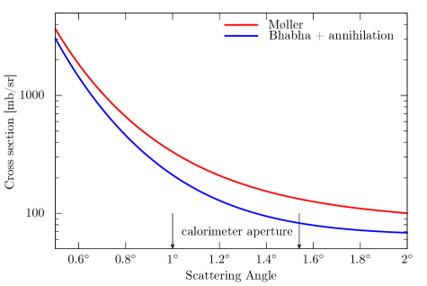
A third advantage is that the actual measured quantity does not change greatly in scale between electron running and positron running. In the MIE analysis, the ratio of countrates is practically the same between species because the $e^{-}p$ cross section is equal to the $e^{+}p$ cross section, absent radiative corrections. In the main analysis, the Møller and Bhabha cross sections differ by nearly a factor of two, as can be seen in figure 6.19. Making a relative luminosity measurement with a given accuracy requires determining that difference with the same accuracy. This is easier to do if the difference is small. Making an accurate determination of the large cross section difference in the main analysis ended up not being possible.

6.6.2 Improvements for Future Implementations

OLYMPUS has been an excellent demonstration that the method is sound, and that future lepton sign asymmetry experiments would do well to take advantage of this techinque for luminosity monitoring. However, the MIE analysis was still only an afterthought. It could have been even more accurate had it been the focus of the SyMB design. The obvious changes to the SyMB hardware that could have improved the MIE analysis all involve the dynamic range of the histograms. If the histogram ranges had all been slightly wider, the (1,3) peak could have been visible in other histograms. This would have allowed cross checks of the effect of the trigger and veto conditiions. Furthermore, the left/right symmetry of the detector system could have been exploited had the (3,1) peak been visible. Extracting luminosity from two different MIE analyses could have provided constraints on beam position and geometry systematics.

Chapter 7 Track Reconstruction

7.1 Overview

Track reconstruction is the task of determining particle trajectories, “tracks” in shorthand, from the unprocessed OLYMPUS data. The task can be divided into two component problems: first, determining how many tracks are in an event and second, estimating, for each track, the particle’s vertex and initial momentum vector. I will refer to the first component problem as “tracking finding” and the second as “track fitting”, and describe our solutions to each in the following sections.

The drift chambers were the main tracking detectors in the OLYMPUS spectrometer. The drift chamber data for each event came in the form of TDC times associated with the different sense wires in the chambers. These times were translated into definite positions along a trajectory, first with some initial processing (described in section 7.2) and then using a time-to-distance (TTD) function (described in section 7.5). Some of the information from the ToFs was also used in track reconstruction. The specific ToF bar hit by a particle gave some position information about its scattering angle, and the time difference between TDC signals from the top and bottom PMTs was used to locate the vertical position of the track. The track reconstruction algorithms combined the ToF and drift chamber data in order to find tracks and fit their initial conditions.

7.2 Processing the Drift Chamber Data

Figure 7.1: The TDC distribution from 100 runs of data is shown for sense wire 317. The distribution has the characteristic “church” shape.

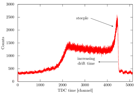
The drift chamber data came in the form of a list of wires that had signals, and then a list of TDC times corresponding to each wire. Some initial processing was needed to convert those TDC times into true drift times. In this section, I will give a description of the initial processing steps.

The distribution of TDC times for a single wire over a run had a characteristic “church” shape, shown in figure 7.1. There was a relatively constant noise floor, a “steeple” at large TDC times, and a “roof” extending to lower TDC times. Because the TDCs were operated in common stop mode, smaller TDC times correspond to longer drift times. The steeple has times produced by tracks that passed very close to the wire. the other end of the church distribution is populated by tracks that passed far from the wire.

The TDC distributions of most wires had, in addition to the church, a pattern of oscillating noise that was in-phase with and had the same frequency as the bunch clock. Our best guess as to the origin of this noise was background originating from adjacent bunches. This noise was not problematic but needed to be accounted for when calibrating the $t_{0}$ times for each wire, as will be discussed in the following sections.

7.2.1 Correcting Trigger Jitter

Figure 7.2: The trigger had some time jitter, as can be seen in the bunch clock TDC spectrum. By subtracting the TDC time for bunch clock pulse corresponding to the bunch that produced the trigger, the common trigger jitter can be removed.

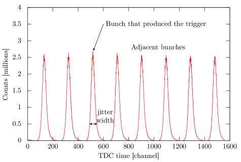
The first processing step was to correct for the time jitter introduced by the trigger. The start signal for the TDC was a current pulse on the sense wire. The stop signal was provided by a delayed trigger signal. The trigger signal had some time jitter, which worsened the drift time resolution. Fortunately, this time jitter could be corrected by using the bunch clock, a simple clock pulse that marked when an accelerator bunch reached the center of the target. We connected the bunch clock as the start signal of an open TDC channel with the same common stop. This produced a distribution like the one shown in figure 7.2. The jitter was removed from the TDC times by subtracting the TDC time of the clock pulse for the bunch that produced the trigger. The jitter-corrected TDC distribution for wire 317 is shown in figure 7.3, and can be compared with the raw TDC distribution of figure 7.1.

Figure 7.3: The jitter-corrected TDC distribution is shown for sense wire 317.

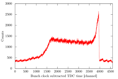
7.2.2 $t_{0}$ Calibration

Figure 7.4: The clean TDC distribution (shown for sense wire 317) was produced by subtracting the periodic noise from between channels 4156 and 4544. This allowed a more stable $t_{0}$ fit.

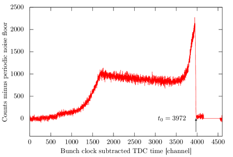
After subtracting the bunch clock, the next step was to find the time of zero drift, or $t_{0}$, for each wire. This time corresponded to tracks that passed directly next to the wire and had zero effective drift distance and zero effective drift time. $t_{0}$ was the baseline TDC time for calculating drift times.

We estimated $t_{0}$ to be the TDC time at which the steeple met the noise floor in the TDC distribution. This point was obscured by the oscillating 10 MHz noise. Since the noise had a well-known frequency and phase, we could subtract it from the TDC distribution, create a “clean” distribution, shown in figure 7.4. We then found the point on the steeple corresponding to 80% and 20% of the steeple height, and extrapolated to the noise floor to find $t_{0}$.

7.3 Track Finding Using Pattern Matching

Figure 7.5: This example data pattern (left panel) has one track as well as several noise hits. The library pattern it matches (right panel) only contains the cells (and ToF bars) hit by the track.

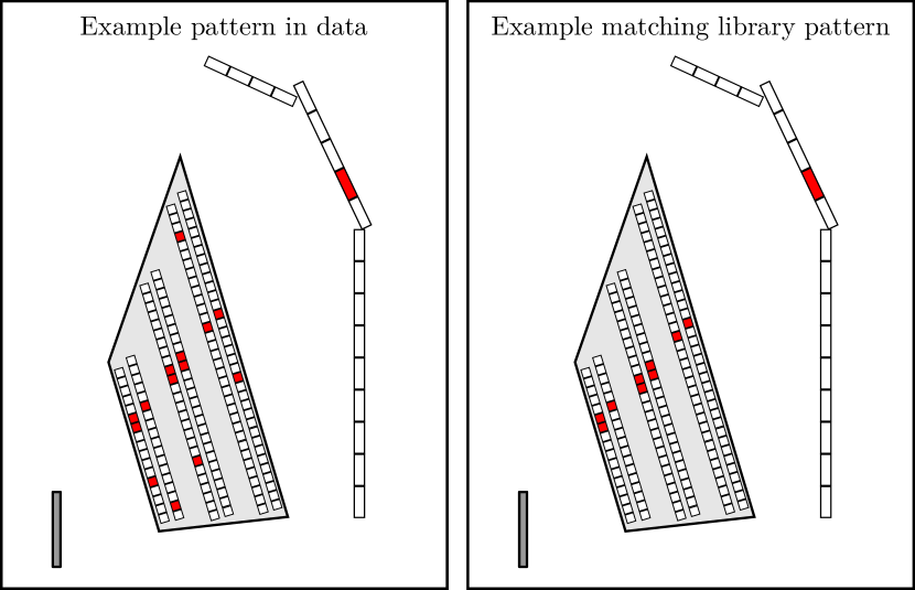
We chose to approach track finding in a different way than the method pursued at BLAST. At OLYMPUS, the beam energy was higher, the accelerator had a lower duty factor, and the beam halo produced by the target was greater. As a consequence, the background environment was worse, especially in the inner chambers of both sectors. We needed some way to reject noise hits that did not come from tracks emerging from the target, and to do so quickly, without trying every combination of hits in all chambers. Our track finding approach was based on the fast pattern matching algorithm of Dell’Orso and Ristori [102]. In their paper, they modeled a particle physics detector as having segments which either made a detection or did not. In our implementation, shown in the example in figure 7.5, each segment was a single drift cell. If at least one wire produced a valid TDC time, then the cell was considered hit. By using cells as the smallest discrete element, we avoided mixing the time-to-distance problem with the pattern matching problem. In addition to drift cells, we also added the ToFs into the pattern matching scheme; if both PMTs in a bar produced a signal, then the bar was considered hit. A single sector of the spectrometer had 159 drift cells and 18 ToF bars. Consequently, our patterns were 177 bits long.

The pattern matching algorithm required a library of patterns corresponding to valid tracks. We generated a library using simulated tracks (see section 8.2.1 for more detail) with a wide range of initial vertices, angles, and momenta. Each library pattern had at least one hit cell in each drift chamber super-layer, and at least one hit ToF bar. Initially, we planned to match separate pattern libraries for the different particle species ($e^{+}$, $e^{-}$, $p$, $\pi^{+}$, etc.), but the libraries overlapped so extensively that we combined them into a single pattern library. The libraries for the two sectors, which were very nearly identical, were also combined. The result was a library of approximately 270,000 patterns.

Figure 7.6: The sub-pattern (right panel) contains a subset of the hit cells in the super-pattern (left panel). Only the super-pattern need be considered by the track fitter.

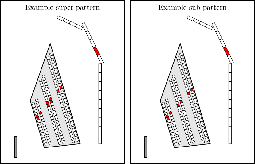
When reconstructing a single event, after the initial data processing and identifying which wires and ToF bars had valid TDC times, pattern matching was performed on each sector. The data pattern was compared against the simulated pattern library, and a list of library matches was produced. In order for a library pattern to be a match, all of its hit cells needed to be hit in data. Stated another way, the bitwise-AND of the library pattern and the data pattern needed to be equal to the library pattern. Each matching library pattern was considered to be a track candidate, with the exception of matches that were “sub-patterns” of other matches. Sub-patterns contained a subset of the hits of another matching pattern, and there was thus no need to produce an additional track candidate. An example of a sub-pattern is shown in figure 7.6.

7.3.1 Modifications to Handle Inefficient Regions

This pattern matching scheme needed to be modified in order to cope with drift chamber cells that were inactive, or slightly inefficient. There were two drift cells that were completely inactive. Though these cells never produced any signals, for the purposes of pattern matching these cells were always considered to have been hit. Tracks that passed through the dead cells were still successfully matched.

Several regions of the drift chambers were found to be slightly inefficient. This presented a potential problem in pattern matching because the library patterns might expect a hit in an inefficient region that might not be present in the data. To cope with this, we modified the criterion for a successful match. Instead of requiring that the bitwise-AND of the data pattern and library pattern equal the library pattern, we required that the bitwise-AND of the data pattern and library pattern have at most one cell missing from the library pattern.

7.4 Track Fitting with the Elastic Arms Algorithm

Each track candidate—the set of TDC times from the cells (and ToFs) matching a library pattern—was fit using an algorithm based on the Elastic Arms Algorithm (EAA) of Ohlsson, Peterson, and Yuille [103, 104]. EAA represents an approach different from what was used successfully at BLAST and was chosen to cope with the challenges specific to OLYMPUS, namely worse position resolution due to higher drift velocity in the drift chambers, and an increase in noise. At BLAST tracks were reconstructed using a microscopic approach. Hits were linked within a super-layer based on linearity and combined with the adjacent super-layer if the resulting track “segment” pointed back toward the target. In this way, smaller units were aggregated until the track was found. At OLYMPUS, left-right ambiguities (first mentioned in section 3.5.1) in a cell were not always resolvable given the limited position resolution. Our algorithm used a macroscopic approach that considered all of the hit positions simultaneously in order to find the likeliest initial conditions for the track.

The problem of track fitting was to estimate, for a given candidate, the likeliest initial conditions. The space of initial conditions was four dimensional; neglecting any transverse motion of the beam, a track was determined by its vertex position $z$, its scattering angle $\theta$, its azimuthal angle $\phi$, and its momentum $p$. The fit of these four parameters was guided by the vector of hit positions $\vec{x}=\{x_{0},x_{1},\ldots x_{i}\ldots\}$ from the various wires and ToF bars in the candidate pattern. A simple fit to find the values of $\{z,\theta,\phi,p\}$ that best match the hit positions $\vec{x}$ could not work because of the problem of left-right ambiguities. A single TDC time in the drift chambers could correspond to two different hit positions, one to the left of the wire and one to the right. Furthermore, some track candidates had some noise hits that did not truly belong to the track, but were part of the matched pattern. EAA was equipped to handle noise rejection. An extension of the original EAA algorithm was specifically designed to work with ambiguities in hit positions [105].

Figure 7.7: The Elastic Arms Algorithm is demonstrated with a simplified example. The space of track initial conditions is one dimensional, represented by the $x$ axis. There are three detector planes; hit positions on these planes are denoted $x_{0}$, $x_{1}$, and $x_{2}$. The detector planes have a left-right ambiguity; the true hit positions are shown as black circles and the false hit positions are shown as blue circles. The sense wires in this example have some staggering, causing the false hit positions to no longer appear in a straight line. The algorithm finds the track coordinate that minimizes an effective potential energy, $E_{eff}$, shown at the bottom of each panel. At high temperature (left panel) there is a single global minimum, which suggests a track that is halfway between the false and true hits. At medium temperature (middle panel) the minimum splits in two, and the true hits are slightly preferred. At low temperature, the most likely track points through the true hits, and the false hits are rejected as noise. As a general trend, as the temperature decreases, there become more local minima, but the minima become narrower.

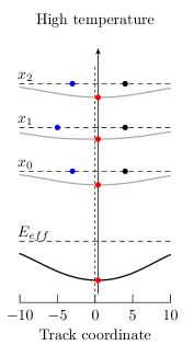
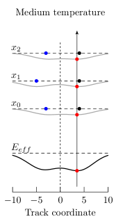
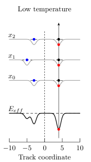
The EAA algorithm, demonstrated with a simplified example in figure 7.7, is a type of annealing filter. In analogy to the physical process of annealing a crystal, the algorithm has a “temperature” parameter, $\beta$, which varies over the course of a fit. Early on, $\beta$ is small, implying a high temperature; the algorithm is more tolerant of hit positions that do not quite match those of the best-fit track. As the algorithm progresses, $\beta$ is increased, reducing the temperature; the algorithm becomes more stringent and rejects hits that are too far from the best-fit track position. In addition to $\beta$, there is also a parameter $\lambda$, which determines the cost for rejecting a hit as noise. Early on, the penalty is high, encouraging the algorithm to be more tolerant and giving every hit a chance to influence the fit. Gradually this penalty is reduced, allowing the algorithm to reject the hits that do not lie along the track. The idea behind the algorithm is that the likeliest initial conditions are specified by the low-temperature global minimum of the fit. However, at low temperatures there are many local minima. At very high temperature, there is only one minimum. By finding the high-temperature global minimum, and by staying in the global minimum as temperature is reduced, the correct low-temperature global minimum can be found.

The word “elastic” in “Elastic Arms Algorithm” does not refer in any way to elastic scattering. Rather, an “elastic arm” is the name given to a deformable track template, essentially a map from initial parameters $\{z,\theta,\phi,p\}$ to track positions $\vec{x}$. The template should be “elastic” in the sense that $x_{i}$ is a continuous and differentiable function over the domain of the initial condition space $\{z,\theta,\phi,p\}$. In an experiment without a magnetic field, particle tracks are straight, and it easy to specify track positions as a function of initial conditions. At OLYMPUS, the magnetic field was non-uniform, we needed a more sophisticated approach. We considered using a deterministic numerical simulation of the trajectories, but this proved to be too computationally intensive and severely limited the speed of the track fitting. Instead, we pre-computed trajectories on a grid over the four-dimensional space of initial conditions, and used cubic spline functions to interpolate between grid points. The result was a set of continuous and differentiable functions $x_{0}(z,\theta,\phi,p)$, $x_{1}(z,\theta,\phi,p)$, $x_{2}(z,\theta,\phi,p)\dots$ that allowed us to forward propagate a guess of initial conditions to estimates of the hit positions on each detector layer. We named this procedure of determining track positions with pre-computed functions “FastTrack.” The FastTrack functions were suitable elastic arms for EAA.

Since the energy loss of electrons and protons in passing through matter is slightly different, we developed a different set of FastTrack functions for each particle type. We found that we could combine the electron and positron functions by remapping the initial conditions. If we replaced $p$ with $1/p$, then an electron with infinite momentum and a positron with infinite momentum both mapped to $1/p=0$. By allowing $1/p$ to have positive values for positrons and negative values for electrons, the fit could start with a lepton of ambiguous charge and fit the lepton charge to the data. We used this procedure as well for proton fits, acknowledging that any track that had anti-proton-like curvature was most likely that of an electron.

7.4.1 Escaping False Minima Using Jump-Scans

We could study the performance of the track fitter by attempting to reconstruct simulated data. We found that even if the drift chambers had perfect time-resolution, some fraction of events were mis-reconstructed. In this case, by mis-reconstructed, I mean that the algorithm resolved at least one left-right ambiguity incorrectly, and fit the track to at least one false position, skewing the estimated initial conditions. Rebecca Russell is certainly the expert on matters relating to track reconstruction improvement [81], but I did contribute one idea which was implemented for the final track reconstruction of the OLYMPUS data. I named this component of the fitting algorithm “Jump-scan”.

In a typical mis-reconstructed event, the fit becomes trapped in a local-minimum. The global minimum is still the correct solution; however, the high-temperature global minimum is not connected to the low-temperature global minimum. To try to prevent this, the algorithm pauses at an intermediate temperature, then tries jumping out of its current minimum and scanning the neighborhood to find a better minimum. After these attempts, EAA proceeds using the best minimum found.

Figure 7.8: This figure shows two trials (out of 48) during Jump-scan, with each step being represented as a circle on the $\theta,\phi$ plane. The trial in the top plot fails to find a better minimum, returning to the minimum of the starting point. The trial in the bottom plot finds a better minimum, and EAA will continue from this minimum at the conclusion of Jump-scan.

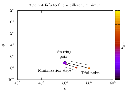
Jump-scan works in the following way. At the chosen intermediate temperature $\beta_{j}$, the algorithm will have a best guess for the initial conditions, $\{z_{j},\theta_{j},\phi_{j},p_{j}\}$. The algorithm will try minimizing from 48 nearby points to see if a better minimum can be found. The algorithm will jump from $\theta_{j}$ to $\theta_{j}-10^{\circ}$, $\theta_{k}-5^{\circ}$, $\theta_{j}+5^{\circ}$, and $\theta_{j}+10^{\circ}$, since mis-reconstructed tracks often have reconstructed scattering angles that are similar to their true scattering angles. Reconstructed $\phi$ and $p$ are often wildly off, so rather than jumping to nearby values, we scan over $\phi=-8^{\circ},0^{\circ},8^{\circ}$, and $1/p=-1/0.083$ GeV^-1, $-1/0.250$ GeV^-1, $1/0.250$ GeV^-1, $1/0.083$ GeV^-1. Reconstructed values of $\theta$ and $z$ are heavily correlated, so we choose only to vary $\theta$, and to keep $z=z_{j}$. This reduced the search space to three dimensions instead of four. At each of the 48 trial points, we minimize to the nearest local minimum. We then compare the minima, move to the best one, and continue the EAA procedure. An example of how this might proceed is shown in figure 7.8.

Jump-scan was an inelegant fix, but it was pragmatic. We found that it improved the perfect reconstruction rate of simulated tracks from about 90% to over 99%. The cost, however, was that it dramatically slowed down the track reconstruction rate. Jump-scan had to be applied to every track in order to be effective. There was no way to know (without trying Jump-scan) if the reconstruction had gone awry and a better minimum could be found. We never succeeded in finding a better fix, balancing the goals of fast reconstruction and a low mis-reconstruction rate.

7.5 Time-to-Distance in the Drift Chambers

7.5.1 Overview

In order for track fitting to be successful, it was crucial to have an accurate a set of time-to-distance (TTD) functions that could translate drift times into drift distances. These functions are approximately linear over a large range of times; a slightly longer drift time implies a slightly longer drift distance. However, close to the sense wires and far from the sense wires, drift time and drift distance cease having a linear relationship. There are several other complications. TTD functions have a dependence on the incident angle, $\alpha$, of the track relative to the wire plane as well as a weak dependence on the azimuthal angle $\phi$ (the functions can vary slightly in the direction parallel to the sense wires). The magnetic field introduces what is called a Lorentz angle to the drift direction; the drift electrons travel at an oblique angle to the electric field, and this angle depends on the magnetic field strength. Since the magnetic field of the spectrometer is non-uniform, every wire has a different time-to-distance relationship. Even the left and right sides of a wire have different TTD functions. What we want to specify is therefore a function $d$ for each side $s$ of every wire $w$:

$$d_{w,s}(t,\alpha,\phi).$$ (7.1)

There are two properties of the TTD functions $d_{w,s}(t,\alpha,\phi)$ that can be easily surmised:

1. $d_{w,s}(0,\alpha,\phi)=0$, i.e., zero drift time implies zero drift distance, regardless of $\alpha$ and $\phi$,

2. $d_{w,s}(t,\alpha,\phi)$ should monotonically increase with $t$, i.e., longer drift time should always imply longer drift distance.

Figure 7.9: This figure shows the drift lines in a drift chamber cell, as calculated by a numerical simulation. The drift distance in the TTD function is reckoned from the point at which the track crosses the sense wire plane, shown in circles for an example track. The TTD function depends on $\alpha$, the incidence angle of the track. The magnetic field caused the electrons to drift at an oblique angle, $\Lambda$, with respect to the electric field, which points along $x$ in this coordinate system. Reversing the magnetic field direction would also reverse the direction of the Lorentz angle.

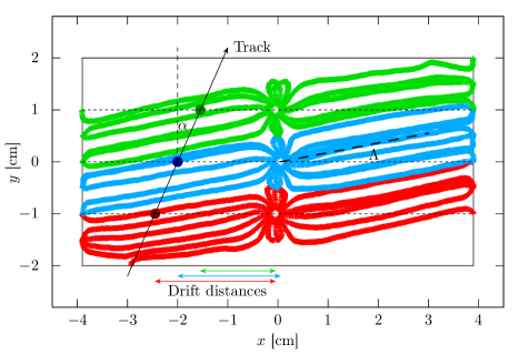
For the reader to become familiar with the TTD in the context of OLYMPUS, I show a simulation of the lines of drift in a typical drift chamber cell in figure 7.9. As in figures 3.8 and 3.9, I show a cross section of the drift cell, so that the wires point in and out of the page. The electric field points parallel to the $x$ direction. However the drift lines are rotated by the Lorentz angle, which I’ll denote as $\Lambda$, relative to the $x$ direction. An example track is shown with an angle of incidence, $\alpha$ relative to the wire planes. We define the drift distance, $d$, as the distance between the sense wire and the intersection of the track with the wire plane. The drift time, $t$, is the time between the passing of the track and the arrival of the first ionization electrons at the sense wire.

In the following sections I will describe three approaches we tried in order to ascertain accurate TTD functions. The first two approaches were unsuccessful, but the third succeeded. In the first approach, we attempted to calculate the TTD functions using an open-source software package called Garfield$++$ [106]. In the second approach, we attempted to ascertain TTD functions from data, and to describe them using general spline functions. In the third, successful approach, we developed a simple parameterization for the shape of a TTD function for the OLYMPUS drift chambers, and fit the parameters of the model using data.

7.5.2 TTD from Garfield

Garfield$++$ is an open source software package developed by CERN to allow customized simulations of tracking detectors. It is written in C$++$ and builds on a previous implementation written in Fortran. There is a wide range of simulations that Garfield$++$ can perform, both with two and three dimensional geometries. We attempted to calculate TTD functions using the following approach. First, we specified the gas mixture and used Garfield$++$’s implementation of the software Magboltz [107] to calculate the response of ionization electrons to electric and magnetic fields in that mixture. Next, we specified the two-dimensional geometry of a row of drift cells, the potentials on all of the wires, and the local magnetic field. Then, we used Garfield$++$ to simulate the two-dimensional drift of ionization electrons from every part of the cell to the sense wires. Lastly, we synthesized the drift time information from the simulations to create TTD functions. We performed this procedure for every drift cell, taking care to specify the local magnetic field of each cell.

This approach did not produce good results. First, we did not precisely know the gas mixture, since the ethanol concentration varied over time (see figure 3.10). We ran simulations with a range of ethanol concentrations, and tried to match different parts of the dataset with different concentrations, but this never yielded a convincing set of TTD functions. Our calculated TTD functions also suffered because we had to assume a nominal description of the geometry. The slight differences in wire positions and voltages between reality and the simulation contributed to the TTD functions’ inaccuracy. In addition to these challenges, our choice of a two-dimensional simulation prevented us from calculating any of the TTD dependence on $\phi$. We could have attempted a three-dimensional simulation, but without having confidence in our approach, we moved on to a different strategy: extracting TTD functions from data.

7.5.3 Spline Fits to Data

Figure 7.10: By making a guess at the TTD functions, we could run the track reconstruction and compare the resulting track positions with the times from data to improve our guess. In this plot, color indicates the incidence angle, $\alpha$, of the reconstructed track.

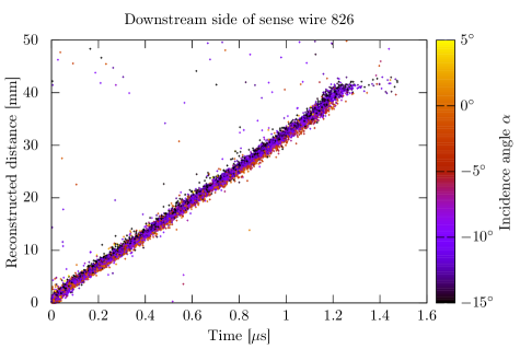
The strategy of our second approach was to iteratively fit TTD functions to data. We started with a set of guess TTD functions so that we could run the track reconstruction over data and produce a set of reconstructed tracks. The track positions could be compared with the drift times in the data to update our TTD functions. An example of such a comparison, made for one side of one sense wire, is shown in figure 7.10. This procedure could be iteratively performed until the TTD functions converged to a solution.

For this approach to work, we needed to choose a functional form for our TTD functions. We chose cubic spline functions, an extremely general choice that put no constraints on the shape that the TTD function could take. Our hope was that the spline functions could easily accommodate slight deviations produced by differences in the wire positions or changes in the magnetic field along the length of the wire.

Figure 7.11: The top plot shows the coplanarity distribution of track pairs for one particular spline solution. The TTD function introduced a bizarre oscillation into the distribution as a function of lepton-scattering angle. For comparison, the bottom plot shows the coplanarity distribution produced when using the TTD function described in section 7.5.4.

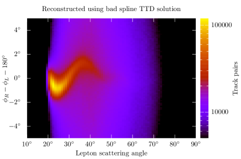
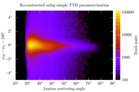
Using this approach, the TTD functions always converged to a solution after a few iterations. However, the quality of these solutions was suspect. With the functions having so much freedom, it was easy for them to converge to a solution that was not a global optimum. As an example, in one such solution the mean of the coplanarity distribution of lepton and proton track pairs oscillated by several degrees as a function of the lepton scattering angle, shown in the top plot of figure 7.11. The origin of this oscillation was determined to be a set of faulty ToF timing calibrations that biased the track reconstruction. When the calibrations were corrected, and TTD fitting iterations were resumed, the oscillations persisted. This indicated that stable non-optimal solutions were possible for the TTD parameters, which meant that quality of the initial TTD guess was critically important. We would have had more confidence in the fitting procedure if the many different initial guesses all converged to the same solution. Instead, we began to worry about how to gauge the quality of various TTD guesses.

Figure 7.12: The spline fits could over-fit the data in regions where the data was sparse. For this particular wire, the function does not monotonically increase, which is problematic.

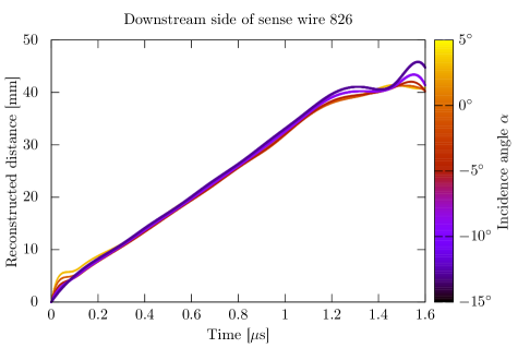
Another reason to be suspicious of the spline functions was that they did not necessarily monotonically increase with increasing time. The spline functions would frequently have regions, especially with large drift times, in which longer times could imply shorter distances. This was caused by the lack of residual data with large drift times. In regions with dense data, the splines were constrained to be well-behaved. In regions where the data was sparse, the splines had the freedom to overfit the data and exhibit wild behavior. This can be seen in figure 7.12, which shows the spline fit to the data of figure 7.10. If we had found an effective way to regularize the splines, then perhaps this approach would have yielded accurate TTD functions, but instead we chose to pursue a third approach, which was ultimately successful.

7.5.4 Simple Parameterization Fit to Data

In our most successful approach for determining time-to-distance functions, we first made a simple parameterization for the shape of a function, and then fit the parameters for each side of each wire to reconstructed data. We tried to choose a shape that matched all of the qualitative features that we observed in reconstruction data, but that lacked the freedom to overfit sparse regions of data. To guide our parameterization, we started with a simple two-dimensional geometric model, and then allowed the parameters of that model to vary quadratically in $\phi$. A derivation of the parameterization is given in appendix C.

The simple parameterization is defined piece-wise into three distinct regions. For times smaller than 0.2 $\mu$s, the function was a cubic polynomial in $t$. For intermediate times, the function was linear in $t$. For large times, the function had a constant value, $d_{\text{max}}$. The parameterization had 10 free parameters, with physical interpretations:

$$v(\phi) =v_{0}+v_{1}\phi+v_{2}\phi^{2}$$ representing the drift velocity (7.2)

$$w(\phi) =w_{0}+w_{1}\phi+w_{2}\phi^{2}$$ representing the width of the jet of drift lines (7.3)

$$\Lambda(\phi) =\Lambda_{0}+\Lambda_{1}\phi+\Lambda_{2}\phi^{2}$$ representing the Lorentz angle (7.4)

$$r \text{representing the radius of the non-linear region}.$$ (7.5)

The parameters were iteratively fit to reconstructed tracks. We started by fitting the parameters to results of a Garfield$++$ simulation. Then using that initial guess, we reconstructed a set of tracks, and then updated the TTD parameters. Each side of each sense wire was allotted its own set of parameters. Furthermore, we divided the OLYMPUS data into segments in time based on the approximate ethanol concentration in the drift chambers and fit the TTD parameters of each segment separately. We found that the TTD parameters converged to a stable solution within about five iterations. An example TTD function is shown in figure 7.13.

Figure 7.13: The TTD functions of the simple parameterization were well-behaved even after fitting the free parameters to data.

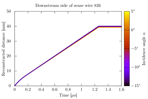
The simple parameterization had desirable properties. The parameters could vary to accommodate slight differences between drift cells, but the TTD functions remained constrained and well-behaved. The kinematic distributions of reconstructed tracks were sensible; the coplanarity distribution peaked at $0^{\circ}$ as expected (shown in the bottom plot of figure 7.11) and no longer had bizarre oscillations. The parameterization yielded hit position resolutions on the order of 0.5–1.0 mm, depending on the wire.

The simple parameterization yielded the most effective set TTD functions that we produced. These functions were used for reconstructing tracks for the analysis discussed in chapter 8 and the results shown in chapter 9.

Chapter 8 Analysis

8.1 Analysis Strategy

Figure 8.1: The track reconstruction, elastic event selection, and background subtraction were performed on both data and simulated data using the same software. The final asymmetry I will present is that of data minus that of simulation.

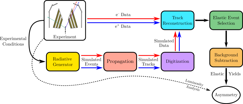
In this chapter, I want to lay out the steps that take the raw data from the experiment and convert them to a lepton sign asymmetry. Some of these steps (for example, the radiative corrections) were described in previous chapters. The goal of this chapter is to both cover the remaining steps, and to orient the reader as to how the entire analysis chain fits together.

In chapter 5, I discussed how the OLYMPUS radiative corrections were necessarily convolved with detector attributes: acceptance, efficiency, resolution. Our solution to this problem is to simulate these convolutions numerically using Monte Carlo, and then to report an asymmetry that is adjusted for the asymmetry we expect to find through simulation. For the sake of clarity, let’s look at some examples in detail, starting with the generator. The events generated in simulation have a slight asymmetry (from soft TPE and from bremsstrahlung interference), which varies with $Q^{2}$. This asymmetry is convolved with, among other things, inefficiency over an area of the detector—say an inactive cell in the drift chambers—since the magnetic field bends electrons and positrons at the same $Q^{2}$ to different parts of the detector. The simulated asymmetry is not caused by hard two-photon exchange, and so must be subtracted from the measured asymmetry.

The general road map for the analysis is shown in the diagram in figure 8.1. In this map the chain moves from the experiment itself, top left, to the result, the asymmetry, at the bottom right. The experimental conditions (beam position, target density, detector settings, etc.) from the experiment serve as input settings to the radiative generator, described in section 5.3. The generator produces simulated events: lists of particles, their vertex, and their momentum vectors. At the next stage, the “propagation”, the trajectories of these particles are simulated, taking into account the particles’ response to magnetic fields and the physical matter of the spectrometer. The simulated trajectories, also called “tracks,” pass next to the “digitization”, which simulates the detector signals that would be produced in order to create simulated data in the exact same format as the experimental data. The data are fed to the track reconstruction (the subject of chapter 7), which tries to invert the processes of digitization and propagation, attempting to find the likeliest of initial conditions for a particle, given the set of detector signals in an event. The reconstructed events are fed next to a piece of software that performs an elastic event selection. This software acts like a filter, accepting events whose reconstructed initial conditions fit those of an elastic collision and rejecting those that look like background. This filter is not perfect, and some residual background must be estimated and subtracted. The result is yields of elastic events, binned as a function of $Q^{2}$ (or $\epsilon$ or $\theta_{l}$, or whatever kinematic variable one chooses.) The experimental and simulated yields are combined with the results from the luminosity analysis to form an asymmetry, according to:

$$A_{2\gamma}=\frac{\frac{N^{\text{data}}_{e^{+}p}}{\mathcal{L}_{e^{+}p}}-\frac{N^{\text{data}}_{e^{-}p}}{\mathcal{L}_{e^{-}p}}}{\frac{N^{\text{data}}_{e^{+}p}}{\mathcal{L}_{e^{+}p}}+\frac{N^{\text{data}}_{e^{-}p}}{\mathcal{L}_{e^{-}p}}}-\frac{\sigma^{\text{sim.}}_{e^{+}p}-\sigma^{\text{sim.}}_{e^{-}p}}{\sigma^{\text{sim.}}_{e^{+}p}-\sigma^{\text{sim.}}_{e^{-}p}}.$$ (8.1)

In the following sections, I will explain, with more detail, how each of these components in the analysis chain works. I will spend particular detail on the elastic event selection, which is solely my own work. A number of my colleagues in the collaboration have designed independent elastic event selection software, with the hope that each independent procedure can help cross check the others. It is anticipated that some combination of these procedures will be used to produce the results that will soon be submitted for publication. I see this chapter as an opportunity to document my design and explain my approach. I will conclude this chapter by mentioning two cross checks of the analysis that can be performed without biasing the result.

8.2 Simulation Chain

In this section, I will describe that chain of software that we used to produce our simulated data set. Even for the simulated data, the first stage in the chain was the experiment. The running conditions of the experiment changed over time while we collected data; the beam position varied slightly, the flow rate of gas into the target was varied, and the settings of the different detectors were occasionally adjusted. To account for this variation, we chose to vary the running conditions of the simulation in exactly the same way as they varied during the experiment. The experimental data are naturally broken up into segments, called “runs”, and we matched the simulation run-by-run to the experiment. For data run 8652, we also produced a simulated run 8652. If the beam moved slightly midway through run 8652, we adjusted the simulated beam position midway through the simulated run 8652. The conditions of each simulated run matched the conditions of each data run.

That does not mean that the events in simulated run 8652 corresponded to any of events in data run 8652. The specific kinematics of each simulated event were generated randomly, and only the running conditions matched the data run. Furthermore, we did not want our simulation to hamper the statistical precision of our result, so the number of elastic events generated for simulation far out-numbered the elastic events in our experimental data set.

The first piece of software in the simulation chain was the radiative generator, which was covered extensively in chapter 5. The output of the generator was, for each event, a vertex position, the momentum vectors for the lepton and proton (as well as the radiated photon, which, for all analyses except that of the SyMB, could be ignored), and a list of weights. These events then passed down the chain to the propagation and digitization stages, which will be described in the following sections.

8.2.1 Propagation

The next step after generating events is to simulate how those events would propagate through the material and magnetic field of the spectrometer. This propagation step takes a particle’s initial vertex and momentum vector and simulates its trajectory. The equations of motion are non-trivial and must be solved numerically. The magnetic field produces curvature in the trajectories, which depends on a particle’s momentum. As particles pass through matter, they lose kinetic energy and, with some probability, can experience secondary scattering. The trajectory is therefore non-deterministic. The simulation should also exhibit this same non-determinism to fully reproduce the characteristics of the experimental data.

The engine of the propagation is an open-source software library, GEANT4 [108], which can numerically and non-deterministically simulate the passage of particles through matter and electromagnetic fields. As inputs to GEANT4, we provide the geometric map of the detector (discussed in section 3.7), and the description of the magnetic field (from the interpolation scheme of section 4.4.1), as well as the list of particles to simulate for each event. We ask, as output from GEANT4, the positions and momentum vectors at important points along a particle’s trajectory (e.g. the wire planes of the drift chambers) as well as other quantities of interest (e.g. the kinetic energy loss in the ToF scintillators).

8.2.2 Digitization

The digitization step converts simulated trajectories from the propagation step and calculates the resulting digital signals that would be produced by our detector electronics. The digitization simulates the TDC and ADC values that our detectors would produce from the simulated track. Just like the generation and propagation steps, this procedure also needs to be non-deterministic.

Each detector system has its own digitization procedure, and, rather than discussing any single digitization scheme in detail here, I will present some illustrative examples of what may be included in such a scheme. For the drift chambers, the task is to take trajectory positions and to determine the corresponding TDC values for drift times to the relevant wires. This step requires inverting the time-to-distance function and applying the correct smearing to the resulting time. For the SyMBs, the digitization requires estimating the ADC signals from the light yield by Cherenkov radiation in the lead fluoride crystals (see Colton O’Connor’s thesis for more detail [83]). For the ToFs, the digitization step includes the simulation of both TDC and ADC signals. The TDC signals must reflect the time-of-flight of the particle as well as the arrival time of scintillation light at the PMTs. The ADC signals must reflect the amount of scintillation light produced and account for attenuation of that light as it travels to the PMTs (see the theses of Lauren Ice and Rebecca Russell for more detail [109, 81]).

All detectors have a probability for being inefficient, i.e., failing to record a signal from a particle that passed through them. This inefficiency is generally random, but can often be correlated over a region of a detector. For example, in many drift chamber cells the three sense wires either all recorded hits from a passing track or all failed to record a hit. Spatial maps of detector inefficiencies, which accounted for correlations, were an important ingredient to the digitization. These maps were estimated from the experimental data, either via alternate or less stringent triggers, and/or by using the track reconstruction to localize particle trajectories at various positions in the detector, which either recorded a signal or did not (for more detail, see Brian Henderson’s thesis [82]).

8.3 Elastic Event Selection

The software that performs elastic event selection acts like a filter, allowing elastic events, the signal, to pass while rejecting background. Generally, it is more important to preserve signal than it is reduce background, simply because if some signal is being discarded, it is difficult to prove that the same fraction is being discarded for both electron and positron data, and in both the experimental and simulated data sets.

Still, removing as much background as possible (without cutting into signal) is important. The final step in the analysis is background subtraction, and an analysis is hardly convincing if the majority of the elastic yield is made up of background contamination. The relationships between the kinematic variables are well-known for the elastic signal (particles have momenta that are strictly correlated with their angles), but the background can come from many different sources, and can have kinematic correlations that are harder to discern. It is better to remove as much background as possible at the elastic event selection phase, than to have to subtract large amounts of an unknown background away.

The most conceptually simple way to segregate signal and background is by using some selection criterion to make a cut, illustrated by the cartoon in figure 5.2. For example, in elastic scattering the sum of the momenta of the lepton and proton must equal the momentum of the beam lepton ($\approx 2$ GeV/$c$ in the beam direction). I choose to set a cut at $1.4$ GeV/$c$: if the reconstructed momenta in the beam direction sum to less than 1.4 GeV/$c$, then I label that event a background event and discard it from my elastic sample. In this section, I will describe the various cuts I choose to make to reduce background.

One pitfall to be avoided, when designing a cutting procedure, is that the cross section changes dramatically over the full range of the OLYMPUS acceptance. If looking at a distribution in some variable, say the sum of reconstructed momenta in the beam direction, the distribution will be dominated by low-$Q^{2}$ events. The rarer high $Q^{2}$ events will be completely obscured. A cut at the ideal position for low-$Q^{2}$ events might remove some high-$Q^{2}$ signal. For that reason, the choice of cut placement must take into account the change in a variable’s distribution over the entire range of $Q^{2}$. I remind the reader that, in elastic scattering at fixed beam energy, there is only one free kinematic variable. Therefore, it is equivalent to consider evolution over $Q^{2}$, or over the proton polar angle, or over any one kinematic variable one chooses. The specific choice of variable is not important, but it is crucial that evolution over some kinematic variable be considered.

Another pitfall to be avoided is the fact that distributions can be slightly different between $e^{-}$ and $e^{+}$ running, between experimental and simulated data, and between the two sectors of the spectrometer. The way that I choose to address this is by making what I call “fitted cuts”. For example, the distribution for the energy of the beam as reconstructed from scattering angles,

$$E_{1}(\theta_{l},\theta_{p})\equiv m_{p}\left(\cot\frac{\theta_{l}}{2}\cot\theta_{p}-1\right),$$

changes depending not only on which slice in $Q^{2}$ one considers, but also on the beam species, on the sector that the lepton traverses, and on whether one is considering data or simulation. The shape of the distribution is approximately gaussian and so by fitting this distribution with gaussian function for many slices of $Q^{2}$, for all of these different conditions, a cut can be made at some number of standard deviations from the mean for each distribution. The advantage is that slight differences in distributions by sector, species, etc. are accounted for. The downside is that the cut position is dependent on the success of a fit, which may be influenced by things like the background contribution, the choice of functional form, or the statistics present in a $Q^{2}$ slice. In some areas of the event selection I believe that this approach is worth the costs, while in some other areas I make simple axis-parallel cuts that are independent of beam species, etc.

In the following subsections, I will go into detail about the procedure I designed.

8.3.1 Finding the Best Pair of Tracks in an Event

Figure 8.2: This cartoon attempts to illustrate the output of the track reconstruction. The left panel shows an event in which a proton traverses the right sector of the spectrometer. The proton induces signals in the detector all along the track. There are also noise signals. The track reconstruction has to interpret those signals and find the likeliest trajectory that could have produced them. In an event such as this, our track reconstruction might output three tracks, as shown in the right panel. The reconstruction identifies the correct hits for the true track, and fits them with both a lepton template (resulting in a positron track) and a proton template. The proton track is a better fit to the detector signals than the positron track. Two of the noise hits also confuse the track reconstruction into thinking that a second particle has passed through the right sector. The reconstruction attempts to fit these signals with a lepton template (resulting in an electron track), and proton template. In this particular example, the reconstruction fails to find a proton solution. The event selection software must cope with the fact that multiple tracks may all correspond to the same original particle.

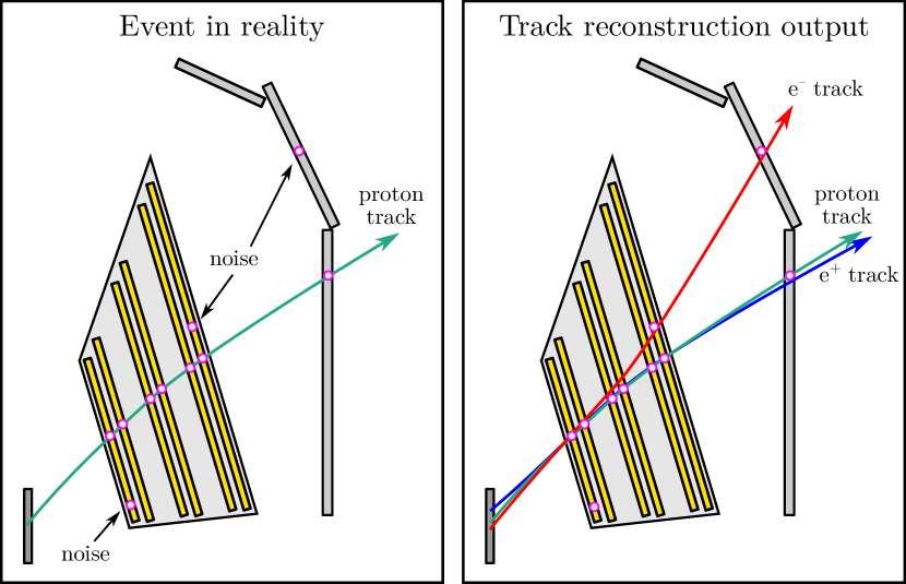
The first stage of the elastic event selection is to find the best pair of tracks in an event. As a consequence of the track reconstruction procedure, multiple tracks might be found, all corresponding to one true trajectory. Figure 8.2 shows a cartoon which attempts to illustrate the behavior of the track reconstruction. Since the reconstruction attempts to fit every track candidate as if it were a lepton and as if it were a proton, the tracks typically come in pairs. Sometimes the combination of signals in data, or some spurious noise close to a trajectory, fool the reconstruction into thinking two particles passed through a sector when only one did. The first stage of the elastic event selection is to sort out the tracks found by the reconstruction and find the best-fit lepton-proton pair from the jumble. This is done by looping over every possible combination of left-sector lepton and right-sector proton, as well as every possible combination of right-sector lepton and left-sector proton, in order to find the best pair.

Loose Cuts

Figure 8.3: Making a set of loose cuts in seven variable dramatically reduces the non-elastic background so that elastic distributions can be more easily fit. The top plot shows all electron-proton pairs, while the bottom plot shows pairs surviving the loose cuts.

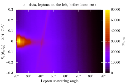
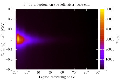
The first step I take at this stage is to make a set of loose cuts in a set of constrained track variables, the effect of which can be seen in figure 8.3. The purpose of this is to reduce the combinatoric background with no loss of signal so that the distributions of elastic events become prominent over background. The space of constrained variables is seven dimensional; making cuts on seven independent variables is sufficient to span the space. For clarity, let us do some dimensional counting. The track reconstruction estimates the momentum vector, and vertex position of a track, for a total of four quantities per track. The time-of-flight scintillator additionally provides the flight time for a total of five per track. An elastic scattering event has two tracks for a total of ten quantities. However, elastic scattering can occur at any value of polar and azimuthal angles, and the vertex position may be anywhere along the target. Of the ten quantities that the reconstruction provides, three of them are free, leaving seven available for making selection cuts. I choose to make loose cuts in the following seven variables (in units where $c=1$):

1. Vertex correlation: $|z_{L}-z_{R}|<100$ mm

2. Azimuthal correlation: $|\phi_{R}-\phi_{L}-180^{\circ}|<6^{\circ}$

3. Beam energy from angles: $|E_{1}(\theta_{l},\theta_{p})-2.01~{}\text{GeV}|<0.3$ GeV

4. Lepton mass-squared from ToF timing: $||\vec{p}_{l}|^{2}(1/\beta_{l}^{2}-1)-m_{e}^{2}|<1$ GeV²

5. Proton mass-squared from ToF timing: $||\vec{p}_{p}|^{2}(1/\beta_{p}^{2}-1)-m_{p}^{2}|<1.5$ GeV²

6. Lepton inverse momentum: $|1/p_{l}-1/p_{l}(\theta_{l})|<1$ GeV^-1

7. Proton inverse momentum: $|1/p_{p}-1/p_{p}(\theta_{p})|<2$ GeV^-1.

The placement of these cuts was designed to be at least five standard deviations from the means over the full range of lepton scattering angles and in most cases the placement is closer to 7–10 standard deviations. After these loose cuts are performed, the elastic events are prominent in the any distribution of kinematic variables, and this allows stable fitting of elastic peaks.

Particle-ID

Figure 8.4: The top plot shows data with positrons in the left sector, after loose cuts have been made. The stripe running through the distribution, at approximately $40^{\circ}$, is made up of combinatoric pairs in which the particle-ID assignments are backwards. This is a problem in positron running, since the positron and proton cannot be distinguished from curvature direction. In the bottom plot, which shows the distribution after particle-ID cuts have been applied, the stripe has been effectively removed.

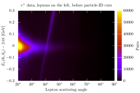
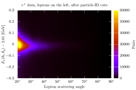
The next step is to remove combinations in which the particle-ID assignments are reversed. The track reconstruction does not attempt to make any particle-ID decisions; every track candidate is fit first as a lepton and again as a proton, and both tracks are provided as output. Therefore, as I step combinatorially over all lepton-proton track pairs, some will consist of a true lepton, tracked as a proton, matched to a true proton, tracked as a lepton. To exclude these combinations, I use timing information from the ToFs to reconstruct a particle’s squared mass from its time-of-flight and momentum.

I choose to make a fitted cut, and furthermore, since the track reconstruction in one sector is independent of the track reconstruction of the other, I know that the lepton mass-squared is reconstructed independently from the proton mass-squared. To fit the distributions, I look at mass-squared as a function of angle in the set of events where the other sector has been heavily restricted. For example, to fit the lepton mass-squared in the left sector, I look at events in which the right sector has a proton which matches the following criteria:

• $||\vec{p}_{p}|^{2}(1/\beta_{p}^{2}-1)-m_{p}^{2}|<0.4$ GeV²

• $|1/p_{p}-1/p_{p}(\theta_{p})|<0.05$ GeV^-1.

This dramatically cleans up the lepton sample in order to make stable fits. To fit the proton distributions, I require that the opposite sector lepton match:

• $|\vec{p}_{l}|^{2}(1/\beta_{l}^{2}-1)-m_{e}^{2}<0.2$ GeV²

• $|\vec{p}_{l}|^{2}(1/\beta_{l}^{2}-1)-m_{e}^{2}>-0.3$ GeV²

• $|1/p_{l}-1/p_{l}(\theta_{l})|<0.03$ GeV^-1.

I fit the distributions in slices of $\theta$ with an asymmetric gaussian plus a constant background. An illustration of a fit for right sector positrons at $\theta_{l}=40^{\circ}$ is shown in figure 8.5.

Figure 8.5: By making hard cuts on the proton in a pair, the lepton mass-squared distribution cleans up dramatically. The peak caused by protons mis-identified as leptons disappears. Notice also that at this angle, the lepton mass-squared reconstructs lower than its expected value of $m_{e}^{2}\approx 0$. This is just one example of distributions that are slightly offset from expectation due to slight bias in the track reconstruction.

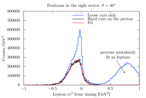
I construct a score for each pair based on the how well the reconstructed masses match the means ($\mu$) and widths ($\sigma$) of the fitted distributions:

$$s_{l}\equiv \frac{\text{max}(m^{2}_{l}-\mu_{l}(\theta_{l}),0)}{\sigma_{l}(\theta_{l})}$$ (8.2)

$$s_{p}\equiv \frac{\text{min}(m^{2}_{p}-\mu_{p}(\theta_{p}),0)}{\sigma_{p}(\theta_{l})}$$ (8.3)

$$s\equiv \sqrt{s_{l}^{2}+s_{p}^{2}}$$ (8.4)

and reject pairs for which $s>5$.

Selecting the Best Pair

The last step at this stage is to pick the best pair of the remaining combinations. It is extremely rare for two independent elastic reactions to occur in the same bunch, and I can safely neglect this case. If two or more pairs survive the loose cuts and the particle-ID selection, usually one of two things is going on. In the first case, the track reconstruction has found two tracks of the correct particle type when only one particle passed through that sector of the spectrometer. This is not terribly worrisome because the track reconstruction usually finds nearly identical momentum vectors for the two tracks. In the second case, there was a simultaneous background track, which should be removed. My approach is to select the best pair based on vertex correlation of the tracks in the two sectors. A background track will have an uncorrelated vertex. In the case of two tracks originating from the same particle, I reason that the one with a vertex that better matches the track on the opposite sector was probably a more successful reconstruction. To select the best pair, I assign a vertex correlation score based on fits to the distributions of vertex correlation, sliced by lepton scattering angle.

8.3.2 Reducing the Inelastic Contribution

Other than the loose cuts, the selection of the best pair enforces no requirements about the elasticity of the event. The particle-ID cuts require that one track was really produced by a lepton and that the other track was really produced by a proton, and the selection based on vertex correlation enforces that the tracks emerged from the same vertex, but the sample at this stage contains both elastic $ep$ events as well as inelastic events. The second stage of the event selection is to reduce the inelastic background. There are still four kinematic criteria that have yet to be leveraged: the beam energy reconstructed from angles, the momentum of the lepton, the momentum of the proton, and the coplanarity (or azimuthal correlation) of the tracks.

Figure 8.6: I make a fitted cut on the beam energy, as reconstructed from angles of the lepton and proton. I’ve illustrated the cut here for positron data in the left sector.

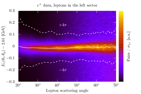
The next cut I make is a fitted cut on beam energy reconstructed from angles, illustrated in figure 8.6. I fit the reconstructed beam energy distribution in slices of lepton scattering angle with an asymmetric gaussian plus a constant background. I discard events in which:

$$\left|\frac{E_{1}(\theta_{l},\theta_{p})-\mu(\theta_{l})}{\sigma(\theta_{l})}\right|>4.$$

Figure 8.7: I find that an axis parallel cut that requires $\sum p_{z}>1.4$ GeV is a simple way to remove inelastic background.

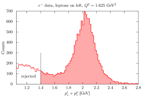
Ideally, I would next use two more fitted cuts based on the momenta of the lepton and proton, but I never found a stable way to fit the elastic peaks in the momentum distributions. In both the lepton and proton momentum distributions, the elastic peaks are not well separated from the inelastic background. However, I did find a combination that was effective at separating background: a cut on the sum of momenta in the direction of the beam (the $z$ direction in the OLYMPUS coordinate system). I make an axis-parallel cut:

$$p_{z}^{l}+p_{z}^{p}>1.4~{}\text{GeV},$$

as shown in figure 8.7. I find that this cut is effective at removing the remaining $e^{\pm}p\rightarrow e^{\pm}\pi^{+}n$ background that persists in the elastic sample. This can be seen in the distribution of the proton mass-squared, shown in figure 8.8.

Figure 8.8: Making a cut on $\sum p_{z}$ helps remove the background in which a pion is reconstructed as a proton. Before the cut (top plot), there is some residual background with a reconstructed mass close to $m_{\pi}^{2}$. After the cut (bottom plot), this background has been eliminated.

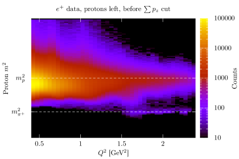
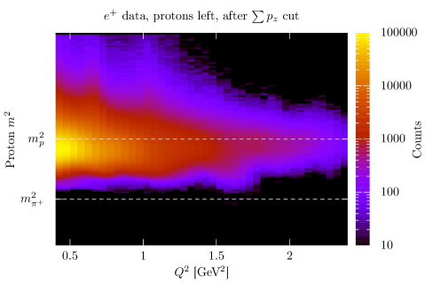
Rather than make a cut on coplanarity, I reserve that distribution in order to estimate the remaining background in my elastic sample.

8.3.3 Fiducial Cuts

Figure 8.9: I make conservative fiducial cuts: the proton azimuthal angle, $\phi_{p}$, was required to fall within $10^{\circ}$ of the horizontal plane, i.e., between the dashed lines. This prevents problems from the slight differences between the experimental acceptance (shown in the top plot) and the simulated acceptance (bottom plot).

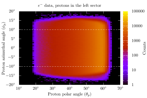
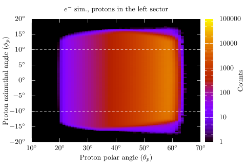
The last stage of the elastic event selection is to make fiducial cuts. The purpose of these cuts is to prevent the effects of acceptance edges from introducing perturbations in the final yields. I only make fiducial requirements on the proton, because the proton reconstruction should be identical for both electron and positron running. I make two fiducial requirements on the elastic events. The first requirement is that the azimuth of the proton be within $\pm 10^{\circ}$ of the horizontal plane ($\phi_{p}=0^{\circ}$ on the left sector and $\phi_{p}=180^{\circ}$ on the right sector. This is shown in figure 8.9. The second requirement is that proton vertex be within 350 mm of the center of the target. The target cell extends to $\pm$300 mm, but I allow an extra 50 mm since the reconstruction of the vertex has some non-zero resolution.

8.4 Background Subtraction

The final step in the analysis chain is to estimate and subtract the remaining background from the elastic yields. For this step, I use the coplanarity distribution. Elastic events are coplanar, while background events need not be. An advantage of using the coplanarity distribution is that the left and right tails of the distribution are the same size. The elastic peak in coplanarity has no skewness.

My approach to estimating the background under the elastic peak is to interpolate between the side-bands of the distribution. The challenge then is to pick a suitable model for the shape of the side-bands. If the background were made up of tracks with random azimuthal angles, then we could expect the background to have a triangular coplanarity distribution (since a triangle is the convolution to two rectangular distributions). If the background still had significant pion contamination, we might expect the coplanarity distribution to be more peaked. What I find is that the side-bands look very flat. This is surprising, and I cannot explain why this might be true. But it certainly makes background estimation a lot easier.

My background estimation procedure is as follows. First, I divide the yields into bins in the kinematic variable of interest (typically $Q^{2}$, $\epsilon$, or $\theta_{l}$). Much like fitted cuts, I fit the background separately for the two species and for the two sectors. For each bin, I fit the elastic peak with a gaussian in order to determine the peak position. I do this to guard against any potential inaccuracy in the track reconstruction. Once I find the peak position, I then fit the side-bands (which I define as $-6^{\circ}$ to $-3^{\circ}$ and from $3^{\circ}$ to $6^{\circ}$ in coplanarity) with a constant-plus-triangle model. I fix the peak of the triangle to be at the same position as the coplanarity peak. I then estimate the background in the signal region (which I define as $-3^{\circ}$ to $3^{\circ}$) by interpolating the constant-plus-triangle model between the side-bands. In practice, I find that the triangular component in the side-band fits is small compared to the constant component, but I still include it because there is no detriment; the fits are very stable. The results of one background fit are shown in figure 8.10.

Figure 8.10: The side-bands of the coplanarity distribution are very flat. The fit indicates a small triangular component as well.

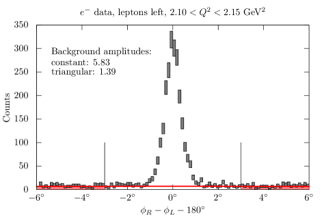
Even though the simulation does not include background subtraction, I perform the same procedure with simulated data anyway. Bremsstrahlung in the radiative generator will cause some elastic events to fall in the side-band region. I want to subtract the same amount of these radiative events from both data and simulation.

Figure 8.11: The background fraction is higher at larger $Q^{2}$, but never exceeds 20%. The background fraction for simulation never exceeds 1%, which is reassuring because the simulation has no background, other than radiative bremsstrahlung events.

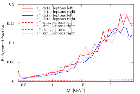
The fractions of background events in both data and simulation are shown in figure 8.11. The background represents a great fraction of the events at larger $Q^{2}$, but never exceeds 20%. The background fraction has the same behavior for both species and both sectors. The background fraction in simulation is much smaller, never exceeding 1%.

The result of background subtraction are final elastic yields (shown in figure 8.12), which can be combined with luminosity information (according to equation 8.1) to form an asymmetry.

Figure 8.12: The yields of elastic events for data and simulation track each other closely over several orders of magnitude.

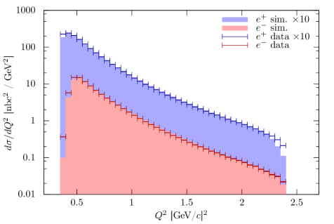
8.5 Cross Checks

It is important to be able to cross check the accuracy of the analysis and to do so without biasing the result. There are numerous opportunities for mistakes to be made: the simulation might fail to match the experiment in some crucial aspect, the track reconstruction can fail to find tracks, the elastic event selection might accidentally throw away some portion of the signal, or the background subtraction fits might fail. Over the years that this analysis chain has been developed and tested, these errors have been identified (and corrected) by investigating the intermediate results: the output from the generator, propagation, digitization, track reconstruction, and event selection. However, once the intermediate results look consistent, it is still possible for problems to be lurking in the final result. How can we build confidence in the asymmetry we report? In this section I will present two ways to cross check the analysis without biasing the final result.

8.5.1 Lepton-Averaged Data vs. Simulation

Agreement between experimental and simulated yields is an obvious test of the analysis. However, the asymmetry we want to measure, will manifest itself as a difference between the experimental data, which may have significant hard two-photon exchange, and simulation, which does not include hard two-photon exchange. Tuning the simulation to match data, in essence, tunes the result. A way to avoid this is by averaging the electron and positron data sets. In the average the hard two-photon exchange will cancel, and then tuning the simulation will not bias the result. Peaks or discontinuities in the ratio of data to simulation indicate that there is still a problem in the analysis that must be solved.

This technique is ultimately limited by our knowledge of the form factors. The lepton-averaged yield amounts, essentially, to an absolute cross section measurement. The absolute cross section for $ep$ scattering is known only as well as the form factors are known, which, in the $Q^{2}$-range of OLYMPUS, is only at the level of about 5–10%. While this limits our ability to cross-check the analysis, it implies that OLYMPUS may be able to make an absolute cross section measurement, as long as the systematic errors can be brought under control.

8.5.2 Comparisons of Left and Right Sector Measurements

The OLYMPUS spectrometer is nearly left/right symmetric. Therefore, one can naturally divide the data between events in which the lepton was tracked in the left sector (and the proton in the right) and events in which the lepton was tracked in the right sector (and the proton in the left). Any measurement made for lepton-left events should match that for lepton-right events. A ratio of left and right measurements should be consistent with unity, while also hiding the actual result of the measurement. Deviations from unity indicate areas with problems. By tuning the analysis to reduce left/right discrepancies, one can improve the analysis without biasing any results.

Chapter 9 Results and Discussion

9.1 Binning

In this chapter, I present preliminary results from the OLYMPUS experiment. The data were analyzed according to the procedure laid out in chapter 8, specifically with elastic event selection (section 8.3) and background subtraction (section 8.4) methods that I designed. As I mentioned in chapter 8, multiple procedures for elastic event selection and background subtraction have been developed in parallel so that each procedure can serve as cross check of the others. The results of this chapter have not had the benefit of those cross checks, so are therefore preliminary. It is intended that the results presented here will be superseded by final OLYMPUS results that will be submitted for publication soon.

The results I present have been binned, and before presenting numbers, I want to discuss my choice of binning. The first choice to make is where to place fiducial limits in $Q^{2}$. The spectrometer only accepts a finite $Q^{2}$ range of scattering angles, but the range is not clear cut because the OLYMPUS target is 60 cm long. At very large $Q^{2}$ and also at small $Q^{2}$, there can be acceptance edge effects which produce artificial asymmetries. Rather than trusting the full range of $Q^{2}$ in which elastic events were collected, I choose to limit the results to a narrower range of $Q^{2}$ where I have confidence that the magnitude of any acceptance effects are small.

Figure 9.1: I have chosen the fiducial bounds in $Q^{2}$ by looking for acceptance edge effects in the lepton-averaged data divided by simulation (top plot) and in difference in asymmetry between the lepton-left and lepton-right data sets (bottom plot). In the bottom plot, the error bands represent statistical uncertainties only.

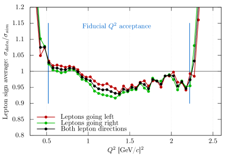
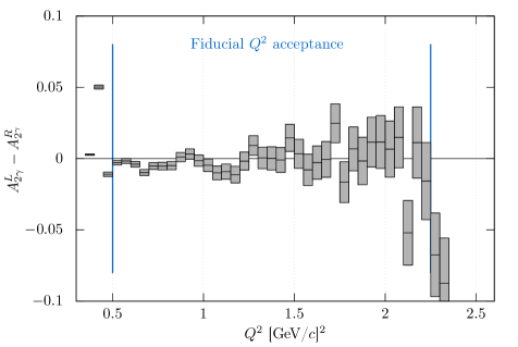
To gauge the placement of fiducial limits in $Q^{2}$, I use the cross checks discussed in section 8.5, and shown in figure 9.1. Using these cross checks, I can make sensible limits on the $Q^{2}$ range without considering the result itself, thereby avoiding a potential source of bias in the results. The first cross check, the lepton-averaged ratio of experimental and simulated cross sections, is shown in the top plot and separated by the lepton sector. For $Q^{2}$ below 0.5 GeV² and above 2.25 GeV², the ratio rises suddenly, indicating edge effects. Outside of these bounds, the experimental acceptance no longer matches the simulated acceptance and the results are not reliable. At intermediate $Q^{2}$, the ratio dips by about 5% below 1. This is not cause for alarm; it reflects uncertainty in the simulated $ep$ cross section. The left lepton ratio mirrors the trend in the right lepton ratio, suggesting the underlying simulated form factors are the cause of the dip. In contrast, for the sudden rise in the ratio at $Q^{2}=2.25$ GeV², the left ratio diverges from the right ratio, signaling an acceptance edge effect.

The second cross check, the asymmetry for left leptons minus the asymmetry for right leptons, is shown in the bottom plot of figure 9.1. In a perfect analysis, the difference between the two asymmetries is zero. As in the lepton averaged ratio, sudden rises or drops indicate acceptance edge effects. From the results of the two cross checks, I believe only results in the range 0.5 GeV² $<Q^{2}<$ 2.25 GeV² are reliable, and so I will only present results in that range.

Figure 9.2: The asymmetry difference between left leptons and right leptons is presented in the binning scheme I use to present results. The fluctuations are much smaller.

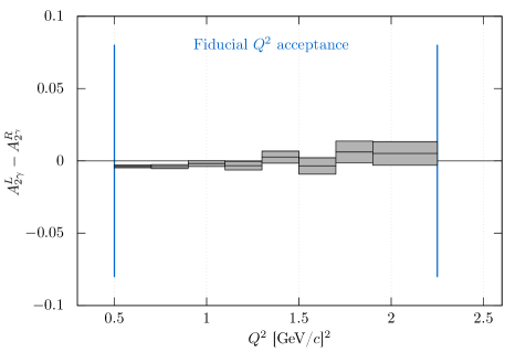
For these cross checks, I have chosen to look at bins that are 0.05 GeV² wide. This is useful for looking at small-scale structures and for acceptance edges, but small bins have the potential for fluctuations, both from statistics, but also from analysis. Slight efficiency dips from dead channels or fluctuations in side-band fits during background subtraction can introduce deviations in small bins that would be washed out in larger bins. Larger bins insulate the result from small scale asymmetries that are not caused by two-photon exchange. This comes at a cost; there is less information about the kinematic trends in the asymmetry if the data are aggregated into fewer wider bins. As a compromise between these two positions, I have chosen to present the result in 8 bins, shown as bins 1–8, in table 9.1. Bins 1–7 are 0.2 GeV² wide, while the last, to accumulate more statistics, has a width of 0.35 GeV². The difference in asymmetry between left leptons and right leptons in this binning scheme is shown in figure 9.2.

Bin	$Q^{2}$	min. $Q^{2}$	max. $Q^{2}$	max. $\epsilon$	min. $\epsilon$
	(GeV/$c$)2	(GeV/$c$)2	(GeV/$c$)2
0	0.165	0.095	0.235	0.9877	0.9675
1	0.60	0.50	0.70	0.9221	0.8813
2	0.80	0.70	0.90	0.8813	0.8346
3	1.00	0.90	1.10	0.8346	0.7818
4	1.20	1.10	1.30	0.7818	0.7230
5	1.40	1.30	1.50	0.7230	0.6581
6	1.60	1.50	1.70	0.6581	0.5874
7	1.80	1.70	1.90	0.5874	0.5113
8	2.075	1.90	2.25	0.5113	0.3667

Table 9.1: This table shows the bin boundaries for the bins in which I will present the OLYMPUS results. The bins are nominally demarcated by $Q^{2}$, and the values of epsilon are calculated assuming a 2.01 GeV beam energy. Bin 0 represents the data point from the $12^{\circ}$ tracking telescopes.

In addition to the eight bins from my analysis of the main spectrometer data, I also include a bin (Bin 0 in table 9.1) for the results from the $12^{\circ}$ tracking telescopes. This analysis was performed by Brian Henderson, and details as well as an error analysis are documented in his thesis [82].

9.2 Systematic Uncertainty

For this preliminary result I will consider systematic uncertainties from only a few sources, and leave conservative estimates for the uncertainties introduced from all others. I choose to divide systematic effects into two categories: effects uncorrelated from bin to bin, and those that are correlated over all of the bins. An example of an uncorrelated systematic effect is a localized error in the simulated acceptance. This will affect the result in the bin corresponding to the affected scattering angle (though this is only approximately true, since we are making a coincidence measurement). An example of a correlated systematic effect is the uncertainty in the species relative luminosity. An error in the relative luminosity will introduce an equal asymmetry to all of the bins. I will break down my estimates in the following sections.

9.2.1 Uncorrelated Systematic Estimate

There are several different sources of uncorrelated systematic uncertainty; species-dependent tracking inefficiency, event selection inefficiency, and uncertainty produced by the background subtraction procedure. For a final published result, each of these sources needs to be studied in detail. For the preliminary result of this chapter, I will make a conservative estimate of the systematic uncertainty by looking at the differences in the lepton-left and lepton-right asymmetries, shown in figure 9.2. I estimate the uncertainty to be the full-scale left-right difference in each bin added in quadrature to an additional 0.5% uncertainty, covering any effects which do not manifest themselves in a left-right asymmetry difference. I choose 0.5%, since that is approximately the scale of the largest left-right difference.

9.2.2 Correlated Systematic Estimate

The most correlated source of systematic uncertainty is the uncertainty on the species relative luminosity. Luminosity differences affect the asymmetry by the same amount for all bins. There are other sources of uncertainty that are correlated over the bins, although not to the same degree. One of those sources is the uncertainty in the true shape of the radiative tails, i.e., whether the true radiative tail is better described using the Method 1 approach (with exponentiation), or using the Method 2 approach (with a single radiated photon) in the radiative generator. As a conservative estimate, I will assign, as a correlated uncertainty, the quadratic sum of the luminosity uncertainty (0.15%) and the full difference between the Method 1 and Method 2 simulated asymmetries.

9.3 Results

Bin	$Q^{2}$	$A_{2\gamma}$	$A_{2\gamma}$	$\delta$ stat.	$\delta$ sys.	$\delta$ sys.
	(GeV/$c$)2	soft from [92]	soft from [89]		uncorr.	corr.
0	0.165	-0.0013	-0.0016	0.0005	0.0027	0.0015
1	0.60	-0.0022	-0.0032	0.0005	0.0063	0.0017
2	0.80	0.0023	0.0014	0.0007	0.0063	0.0018
3	1.00	0.0034	0.0027	0.0010	0.0053	0.0020
4	1.20	0.0044	0.0041	0.0015	0.0060	0.0023
5	1.40	0.0069	0.0069	0.0021	0.0056	0.0027
6	1.60	0.0128	0.0134	0.0028	0.0061	0.0031
7	1.80	0.0058	0.0071	0.0038	0.0080	0.0035
8	2.075	0.0080	0.0105	0.0040	0.0072	0.0044

Table 9.2: This table shows the preliminary lepton sign asymmetry result from OLYMPUS for two different definitions of soft two-photon exchange.

The preliminary results of the OLYMPUS experiment are shown in 9.2. I present two different asymmetries, each corresponding to a slightly different way of making of radiative corrections. The first asymmetry (in column 3) uses the Maximon and Tjon definition of soft two-photon exchange [92]. The second asymmetry (in column 4) uses the Mo and Tsai definition [89]. The two definitions of where to draw the hard/soft boundary are arbitrary, so I present our result for both so that the relevant asymmetry can be used for comparisons. For example, the form factor fits of Bernauer et al. [57] use data that have been corrected (in many cases, retroactively) using Maximon and Tjon. For that reason any comparisons to Bernauer fits will be made with our Maximon and Tjon asymmetry. In contrast, the other contemporary two-photon exchange experiments use the Mo and Tsai definition of soft two-photon exchange, and so I will only compare our Mo and Tsai asymmetry to their results. For clarification, both asymmetries I present use the Method 1 radiative corrections. The difference between Method 1 and Method 2 is included in the correlated systematic uncertainty estimate.

Figure 9.3: The asymmetry with the Maximon and Tjon definition of soft TPE is presented as a function of $\epsilon$ (top plot) and $Q^{2}$ (bottom plot).

Figure 9.4: The asymmetry with the Mo and Tsai definition of soft TPE is presented as a function of $\epsilon$ (top plot) and $Q^{2}$ (bottom plot).

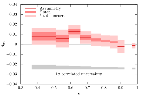
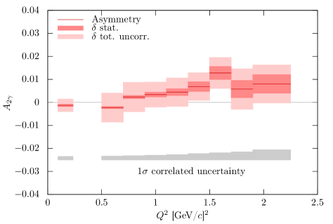
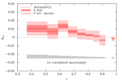
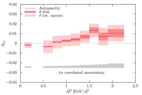
Figures 9.3 and 9.4 show the asymmetries in table 9.2 plotted as functions of $\epsilon$ and $Q^{2}$. Figure 9.3 shows the results using the Maximon and Tjon definition of soft TPE, while figure 9.4 shows the results according to the Mo and Tsai definition. The statistical and uncorrelated uncertainties are shown as colored bands around the measured asymmetry. The correlated systematic uncertainties are shown in a band below.

Qualitatively, the data show an asymmetry that varies over the kinematic range, increasing with $Q^{2}$ and increasing as $\epsilon\longrightarrow 0$. This specific slope indicates that the two-photon exchange contribution reduces the size of the form factor discrepancy. However, the magnitude of the asymmetry is not large: only growing to about 1% at the end of the OLYMPUS acceptance. Many of the points have an asymmetry that is within error of zero. That is partially due to my conservative estimate of the systematic uncertainties. The goal is that by studying the various systematic effects in detail, we can, with confidence, reduce those uncertainties.

9.4 Comparison with Novosibirsk and CLAS

Figure 9.5: The kinematics of the published data points of the CLAS and Novosibirsk two-photon experiments are shown in comparison to the OLYMPUS data points presented in this thesis.

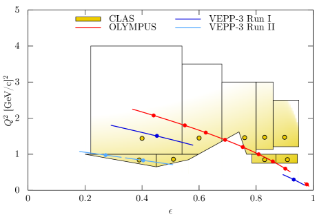
OLYMPUS is not the only contemporary lepton sign asymmetry experiment with new results. Both the experiments in Novosibirsk and at CLAS have recently published results. The kinematic reach of the data from all three contemporary experiments is shown in figure 9.5. In this section, I show the results of the other two experiments, and make a comparison with the OLYMPUS results in this thesis.

9.4.1 Novosibirsk Results

Figure 9.6: The Novosibirsk experiment published four data points, at two different beam energies. The experiment was statistics limited; the systematic errors are nearly invisible in this plot.

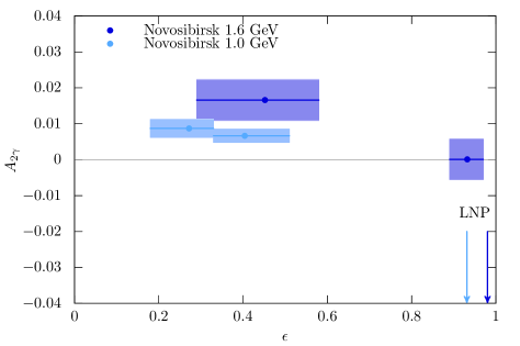
The results of the Novosibirsk two-photon experiment were published in a letter in 2015 [68]. I have rendered the results from this paper in figure 9.6. The Novosibirsk experiment reported four data points, at two different beam energies. The experiment was severely statistics limited; in fact, the quadratic sum of the systematic and statistical error bars is practically invisible in figure 9.6 on top of the statistical-only errors. The Novosibirsk experiment monitored the relative $e^{-}p$ and $e^{+}p$ luminosities through the rate of forward elastic $ep$ scattering. As a consequence, the results are relative to the asymmetry at these luminosity normalization points (LNPs), shown with arrows in figure 9.6.

With only four data points, the Novosibirsk results are hardly conclusive, but are certainly suggestive of a two-photon exchange effect which helps resolve the discrepancy. At both beam energies, the asymmetry rises as $\epsilon$ decreases. Furthermore, at higher beam energy the asymmetry rise is greater, which is consistent with a larger discrepancy at greater $Q^{2}$.

9.4.2 CLAS Results

Figure 9.7: The CLAS two-photon experiment results for their fixed $Q^{2}$ binning scheme are shown. The inner bands for each bin represent statistical error only, while the outer bands represent the quadratic sum of point-to-point errors. The correlated luminosity uncertainty is shown by the gray band below the data.

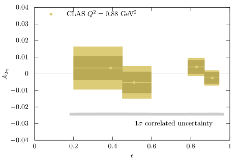
The CLAS two-photon experiment has released results [71], which at the time of this writing are in the midst of the peer-review process. The results were presented in two different binning schemes. In one scheme the bin centers are positioned along lines of constant $\epsilon$, and in the other scheme the bin centers are positioned along lines of constant $Q^{2}$. The bins in the two schemes overlap, and so are not statistically independent. For that reason, in this work I will only show the constant $Q^{2}$ scheme, which allows me to plot variations in $\epsilon$, in figure 9.7. For the constant $Q^{2}$ scheme, the CLAS experiment has released four points at $Q^{2}=0.88$ GeV², and five points at $Q^{2}=1.45$ GeV². Since the experiment used a tertiary beam that had a range of energies, the bins are not contours in the $\epsilon,Q^{2}$ plane, but polygons, and are shown in figure 9.5.

The data at $Q^{2}=0.88$ GeV², shown in the top plot of figure 9.7 are all consistent with zero asymmetry. This is not surprising, because the form factor discrepancy is not large at this $Q^{2}$. The $Q^{2}=1.45$ GeV² data, shown in the bottom plot, have a slight rising trend, as $\epsilon\rightarrow 0$. However, only the lowest $\epsilon$ point has an asymmetry greater than zero by more than the quoted uncertainty.

9.4.3 Comparison with OLYMPUS

Figure 9.8: Only the CLAS and Novosibirsk data close to the $E=2$ GeV contour are plotted for comparison with the OLYMPUS results from this thesis.

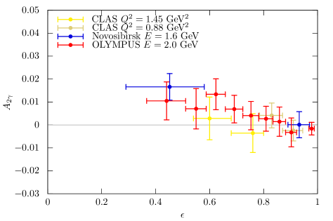
Making a comparison between the CLAS and Novosibirsk data and OLYMPUS is difficult as the three experiments measure slightly different kinematic points as seen in figure 9.5. The three experiments are not measuring the same quantities exactly, and need not agree. In the interest of making a comparison anyway, I observe that a few of the CLAS and Novosibirsk data points fall close to the OLYMPUS points presented in this thesis, and that the results for the three experiments should be similar for this limited set of points. A plot of the asymmetries of these points is shown in figure 9.8. The three experiments are consistent; however, the uncertainties are so large that it would be difficult for that not to be the case.

9.5 Two-Photon Exchange Hypothesis

The OLYMPUS results quantify the contribution to the elastic $ep$ cross section from hard two-photon exchange. The motivation for this measurement, however, was addressing the proton form factor discrepancy. The crucial question is whether or not the OLYMPUS result supports or contradicts the hypothesis that hard two-photon exchange is the source of the discrepancy. This is a difficult question to answer for several reasons. The size of the form factor discrepancy is only as well quantified as the form factors have been quantified via Rosenbluth separation. Measurements of the lepton sign asymmetry at a few kinematic points is not enough to fully constrain the two-photon exchange correction’s dependence on $\epsilon$ and $Q^{2}$. The measurements themselves also have limited precision and accuracy.

It is the purview of phenomenology to determine the asymmetry needed to fully resolve that discrepancy, and there have been several such calculations [38, 41, 42, 57]. In appendix D, I derive a very simple method for estimating the asymmetry from the size of the form factor discrepancy with the help of a few simplifying assumptions. To answer whether the OLYMPUS results are consistent with a resolution with the discrepancy, we should compare the results to these calculations.

Figure 9.9: The OLYMPUS results are compared with three phenomenological extractions of how large of an asymmetry is needed to resolve the discrepancy. The light-blue error band is associated with my estimate using the Bernauer form factor fits, and is described in more detail in appendix D.

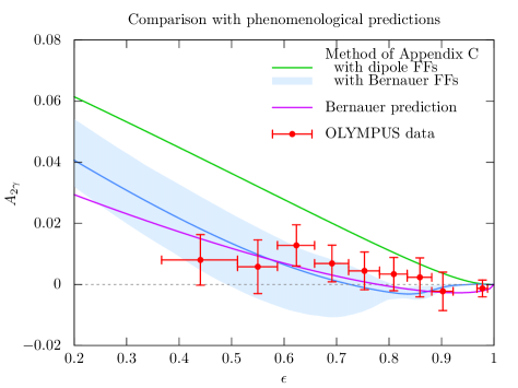
Figure 9.9 shows the OLYMPUS results compared to my simple estimate, for two different form factor models, as well as a more sophisticated estimate by Bernauer et al. [57]. My estimate using dipole form factors predicts an asymmetry that grows much faster than both the OLYMPUS data and the other predictions. This is to be expected, since under the dipole assumption, $\mu_{p}G_{E}/G_{M}=1$, while in many fits to Rosenbluth data, $\mu_{p}G_{E}/G_{M}$ is below 1. The dipole model assumes that the discrepancy is larger than more sophisticated fits suggest.

My simple estimate using the Bernauer form factor fits predicts roughly the same qualitative trends as the Bernauer prediction, which should not be surprising since both estimates use the same underlying form factors. The light blue error band is associated with my simple estimate, and is a way of gauging the uncertainty in the magnitude of the form factor discrepancy. The slope of the OLYMPUS data does not seem to be as great as the phenomenological calculations predict. However OLYMPUS is certainly consistent within the blue error band, and I do not believe that the OLYMPUS results are inconsistent with the two-photon exchange hypothesis.

9.6 Conclusions

OLYMPUS has measured the lepton sign asymmetry over a wide-range of angles, and the results in this thesis are a determination of the hard TPE contribution to $ep$ scattering. The asymmetry has a clear slope, and the direction of that slope suggests a mitigation of the form factor discrepancy. The uncertainty estimates in their current state are conservative, and therefore make it to difficult to draw definite conclusions about whether or not two-photon exchange is the sole cause of the form factor discrepancy, especially since the magnitude of the measured asymmetry is only about 1%. Fortunately, the analysis of the systematic uncertainties will progress and as OLYMPUS nears a final result, the goal is to reduce, with confidence and justification, the size of the uncertainty estimates. With smaller systematic uncertainties, it may be possible for more decisive conclusions to be drawn. It will certainly be interesting once the OLYMPUS data can be combined with the data from Novosibirsk and CLAS in order to make fits and extrapolations of the hard TPE effect.

Appendix A Bremsstrahlung Cross Section

The cross section for tree-level bremsstrahlung is an important component to the radiative generator. In this appendix I will show some important derivations. I have a couple of notational preferences which I will use in this appendix. I will use $\vec{v}$ to refer to a three-vector, but $\overleftarrow{v}$ to refer to four-vectors, whose individual components will be labeled as $v_{\mu}$. The expression $v^{2}$ will mean $v_{\mu}v^{\mu}$, or equivalently $\overleftarrow{v}\cdot\overleftarrow{v}$. The norm of a three vector, defined as $\sqrt{\vec{v}\cdot\vec{v}}$, will be written as $|\vec{v}|$.

I will use the Dirac gamma matrices $\gamma_{\mu}$. I will write contractions of the form $\gamma_{\mu}v^{\mu}$ as $\not{v}$.

A.1 Bremsstrahlung Matrix Element

Figure A.1: There are four tree-level bremsstrahlung diagrams.

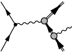
There are four tree-level bremsstrahlung diagrams, shown in figure A.1, whose matrix elements must be summed together. I’ll label these matrix elements as $\mathcal{M}_{li}$, $\mathcal{M}_{lf}$, $\mathcal{M}_{pi}$, and $\mathcal{M}_{pf}$ based on if the photon emerges from a lepton or proton, and an initial or final leg. Let’s call the incoming lepton 4-momentum $\overleftarrow{p}_{1}$, the incoming proton 4-momentum $\overleftarrow{p}_{2}$, the outgoing lepton 4-momentum $\overleftarrow{p}_{3}$, and the outgoing proton 4-momentum $\overleftarrow{p}_{4}$. The 4-momentum of the outgoing photon will be labeled with $\overleftarrow{k}$. Following Feynman rules, the four matrices can be written as:

$$\mathcal{M}_{li}= -e^{3}\epsilon^{\ast}_{\lambda}(\overleftarrow{k})\bar{u}(\overleftarrow{p}_{3})\gamma_{\mu}\frac{\not{p}_{1}-\not{k}+m}{2\overleftarrow{p}_{1}\cdot\overleftarrow{k}}\gamma^{\lambda}u(\overleftarrow{p}_{1})\frac{1}{(\overleftarrow{p}_{1}-\overleftarrow{k}-\overleftarrow{p}_{3})^{2}}\bar{u}(\overleftarrow{p}_{4})\Gamma^{\mu}(\overleftarrow{p}_{4}-\overleftarrow{p}_{2})u(\overleftarrow{p}_{2})$$ (A.1)

$$\mathcal{M}_{lf}= e^{3}\epsilon^{\ast}_{\lambda}(\overleftarrow{k})\bar{u}(\overleftarrow{p}_{3})\gamma_{\lambda}\frac{\not{p}_{3}+\not{k}+m}{2\overleftarrow{p}_{3}\cdot\overleftarrow{k}}\gamma^{\mu}u(\overleftarrow{p}_{1})\frac{1}{(\overleftarrow{p}_{1}-\overleftarrow{k}-\overleftarrow{p}_{3})^{2}}\bar{u}(\overleftarrow{p}_{4})\Gamma^{\mu}(\overleftarrow{p}_{4}-\overleftarrow{p}_{2})u(\overleftarrow{p}_{2})$$ (A.2)

$$\mathcal{M}_{pi}= e^{3}\epsilon^{\ast}_{\lambda}(\overleftarrow{k})\bar{u}(\overleftarrow{p}_{3})\gamma_{\mu}u(\overleftarrow{p}_{1})\frac{1}{(\overleftarrow{p}_{1}-\overleftarrow{p}_{3})^{2}}\bar{u}(\overleftarrow{p}_{4})\Gamma^{\mu}(\overleftarrow{p}_{1}-\overleftarrow{p}_{3})\frac{\not{p}_{2}-\not{k}+M}{2\overleftarrow{p}_{2}\cdot\overleftarrow{k}}\Gamma^{\lambda}(-\overleftarrow{k})u(\overleftarrow{p}_{2})$$ (A.3)

$$\mathcal{M}_{pf}= -e^{3}\epsilon^{\ast}_{\lambda}(\overleftarrow{k})\bar{u}(\overleftarrow{p}_{3})\gamma_{\mu}u(\overleftarrow{p}_{1})\frac{1}{(\overleftarrow{p}_{1}-\overleftarrow{p}_{3})^{2}}\bar{u}(\overleftarrow{p}_{4})\Gamma^{\lambda}(-\overleftarrow{k})\frac{\not{p}_{4}+\not{k}+M}{2\overleftarrow{p}_{4}\cdot\overleftarrow{k}}\Gamma^{\mu}(\overleftarrow{p}_{1}-\overleftarrow{p}_{3})u(\overleftarrow{p}_{2}).$$ (A.4)

Taking the sum of all four, we get:

$$\begin{split}\mathcal{M}_{\text{brems.}}=e^{3}\epsilon^{\ast}_{\lambda}(\overleftarrow{k})\Big{\{}\bar{u}(\overleftarrow{p}_{3})A_{\lambda\mu}(\overleftarrow{p}_{1},\overleftarrow{p}_{3},\overleftarrow{k})u(\overleftarrow{p}_{1})\frac{1}{(\overleftarrow{p}_{4}-\overleftarrow{p}_{2})^{2}}\bar{u}(\overleftarrow{p}_{4})\Gamma_{\mu}(\overleftarrow{p}_{4}-\overleftarrow{p}_{2})u(\overleftarrow{p}_{2})\\ -\bar{u}(\overleftarrow{p}_{3})\gamma_{\mu}u(\overleftarrow{p}_{1})\frac{1}{(\overleftarrow{p}_{1}-\overleftarrow{p}_{3})^{2}}\bar{u}(\overleftarrow{p}_{4})B^{\lambda\mu}(\overleftarrow{p}_{2},\overleftarrow{p}_{4},\overleftarrow{k})u(\overleftarrow{p}_{2})\Big{\}},\end{split}$$ (A.5)

where the tensors $A_{\lambda\mu}(\overleftarrow{p}_{1},\overleftarrow{p}_{3},\overleftarrow{k})$ and $B^{\lambda\mu}(\overleftarrow{p}_{2},\overleftarrow{p}_{4},\overleftarrow{k})$ are given by:

$$A_{\lambda\mu}(\overleftarrow{p}_{1},\overleftarrow{p}_{3},\overleftarrow{k})={} \left[\gamma_{\lambda}\frac{\not{p}_{3}+\not{k}+m}{2\overleftarrow{p}_{3}\cdot\overleftarrow{k}}\gamma_{\mu}-\gamma_{\mu}\frac{\not{p}_{1}-\not{k}+m}{2\overleftarrow{p}_{1}\cdot\overleftarrow{k}}\gamma_{\lambda}\right],$$ (A.6)

$$\begin{split}B^{\lambda\mu}(\overleftarrow{p}_{2},\overleftarrow{p}_{4},\overleftarrow{k})={}&\Bigg{[}\Gamma^{\lambda}(-\overleftarrow{k})\frac{\not{p}_{4}+\not{k}+M}{2\overleftarrow{p}_{4}\cdot\overleftarrow{k}}\Gamma^{\mu}(\overleftarrow{p}_{4}+\overleftarrow{k}-\overleftarrow{p}_{2})\\ {}&-\Gamma^{\mu}(\overleftarrow{p}_{4}+\overleftarrow{k}-\overleftarrow{p}_{2})\frac{\not{p}_{2}-\not{k}+M}{2\overleftarrow{p}_{2}\cdot\overleftarrow{k}}\Gamma^{\lambda}(-\overleftarrow{k})\Bigg{]}.\end{split}$$ (A.7)

To calculate a cross section, we’ll need to square this matrix element. And since we want an unpolarized cross section, we must average the initial spin states and sum over the final spin-states:

$$\left\langle|\mathcal{M}_{\text{brems.}}|^{2}\right\rangle= \frac{1}{4}\sum_{\text{spins}}\left[\mathcal{M}^{\dagger}_{\text{brems.}}\mathcal{M}_{\text{brems.}}\right]$$ (A.8)

$$\begin{split}=&\frac{e^{6}}{4}\sum_{\text{spins}}\Bigg{[}\epsilon^{\ast}_{\lambda}\epsilon_{\kappa}\\ &\bigg{\{}u^{\dagger}(\overleftarrow{p}_{1})A^{\dagger\kappa\nu}(\overleftarrow{p}_{1},\overleftarrow{p}_{3},\overleftarrow{k})\gamma_{0}u(\overleftarrow{p}_{3})\frac{1}{(\overleftarrow{p}_{4}-\overleftarrow{p}_{2})^{2}}u^{\dagger}(\overleftarrow{p}_{2})\Gamma^{\dagger}_{\nu}(\overleftarrow{p}_{4}-\overleftarrow{p}_{2})\gamma_{0}u(\overleftarrow{p}_{4})\\ &-\bar{u}(\overleftarrow{p}_{1})\gamma_{\mu}u(\overleftarrow{p}_{3})\frac{1}{(\overleftarrow{p}_{1}-\overleftarrow{p}_{3})^{2}}u^{\dagger}(\overleftarrow{p}_{2})B^{\dagger\kappa\nu}(\overleftarrow{p}_{2},\overleftarrow{p}_{4},\overleftarrow{k})\gamma_{0}u(\overleftarrow{p}_{4})\bigg{\}}\\ &\bigg{\{}\bar{u}(\overleftarrow{p}_{3})A_{\lambda\mu}(\overleftarrow{p}_{1},\overleftarrow{p}_{3},\overleftarrow{k})u(\overleftarrow{p}_{1})\frac{1}{(\overleftarrow{p}_{4}-\overleftarrow{p}_{2})^{2}}\bar{u}(\overleftarrow{p}_{4})\Gamma_{\mu}(\overleftarrow{p}_{4}-\overleftarrow{p}_{2})u(\overleftarrow{p}_{2})\\ &-\bar{u}(\overleftarrow{p}_{3})\gamma_{\mu}u(\overleftarrow{p}_{1})\frac{1}{(\overleftarrow{p}_{1}-\overleftarrow{p}_{3})^{2}}\bar{u}(\overleftarrow{p}_{4})B^{\lambda\mu}(\overleftarrow{p}_{2},\overleftarrow{p}_{4},\overleftarrow{k})u(\overleftarrow{p}_{2})\bigg{\}}\Bigg{]}.\end{split}$$ (A.9)

We’ll have to drag $\gamma_{0}$ accross the operators $\Gamma$, $A$, and $B$.

For the case of $\Gamma$:

$$\Gamma_{\mu}^{\dagger}(\overleftarrow{q})\gamma_{0} =\left(F_{1}(Q^{2})\gamma_{\mu}+\frac{i\kappa F_{2}(Q^{2})}{2m_{p}}q_{\nu}\sigma^{\mu\nu}\right)^{\dagger}\gamma_{0}$$ (A.10)

$$=\left(F_{1}(Q^{2})\gamma_{\mu}^{\dagger}-\frac{i\kappa F_{2}(Q^{2})}{2M}q_{\nu}\sigma^{\dagger\mu\nu}\right)\gamma_{0}$$ (A.11)

$$=\gamma_{0}\left(F_{1}(Q^{2})\gamma_{\mu}-\frac{i\kappa F_{2}(Q^{2})}{2M}q_{\nu}\sigma^{\mu\nu}\right)$$ (A.12)

$$=\gamma_{0}\Gamma_{\mu}^{\dagger}(-\overleftarrow{q}).$$ (A.13)

For the case of $A$:

$$A^{\dagger}_{\mu\nu}(\overleftarrow{p}_{1},\overleftarrow{p}_{3},\overleftarrow{k})\gamma_{0} =\left[\gamma_{\mu}\frac{\not{p}_{3}+\not{k}+m}{2\overleftarrow{p}_{3}\cdot\overleftarrow{k}}\gamma_{\nu}-\gamma_{\nu}\frac{\not{p}_{1}-\not{k}+m}{2\overleftarrow{p}_{1}\cdot\overleftarrow{k}}\gamma_{\mu}\right]^{\dagger}\gamma_{0}$$ (A.14)

$$=\left[\gamma_{\nu}^{\dagger}\frac{\not{p}_{3}^{\dagger}+\not{k}^{\dagger}+m}{2\overleftarrow{p}_{3}\cdot\overleftarrow{k}}\gamma_{\mu}^{\dagger}-\gamma_{\mu}^{\dagger}\frac{\not{p}^{\dagger}_{1}-\not{k}^{\dagger}+m}{2\overleftarrow{p}_{1}\cdot\overleftarrow{k}}\gamma_{\nu}^{\dagger}\right]\gamma_{0}$$ (A.15)

$$A^{\dagger}_{\mu\nu}(\overleftarrow{p}_{1},\overleftarrow{p}_{3},\overleftarrow{k})\gamma_{0} =\gamma_{0}\left[\gamma_{\nu}\frac{\not{p}_{3}+\not{k}+m}{2\overleftarrow{p}_{3}\cdot\overleftarrow{k}}\gamma_{\mu}-\gamma_{\mu}\frac{\not{p}_{1}-\not{k}+m}{2\overleftarrow{p}_{1}\cdot\overleftarrow{k}}\gamma_{\nu}\right]$$ (A.16)

$$=\gamma_{0}A_{\nu\mu}(\overleftarrow{p}_{1},\overleftarrow{p}_{3},\overleftarrow{k}).$$ (A.17)

Note that the indices of the $A$ tensor have become reversed.

Lastly, for the case of $B$:

$$\begin{split}B^{\dagger}_{\mu\nu}(\overleftarrow{p}_{2},\overleftarrow{p}_{4},\overleftarrow{k})\gamma_{0}&=\Bigg{[}\Gamma_{\mu}(-\overleftarrow{k})\frac{\not{p}_{4}+\not{k}+M}{2\overleftarrow{p}_{4}\cdot\overleftarrow{k}}\Gamma_{\nu}(\overleftarrow{p}_{4}+\overleftarrow{k}-\overleftarrow{p}_{2})\\ {}&-\Gamma_{\nu}(\overleftarrow{p}_{4}+\overleftarrow{k}-\overleftarrow{p}_{2})\frac{\not{p}_{2}-\not{k}+M}{2\overleftarrow{p}_{2}\cdot\overleftarrow{k}}\Gamma_{\mu}(-\overleftarrow{k})\Bigg{]}^{\dagger}\gamma_{0}\end{split}$$ (A.18)

$$\begin{split}&=\Bigg{[}\Gamma^{\dagger}_{\nu}(\overleftarrow{p}_{4}+\overleftarrow{k}-\overleftarrow{p}_{2})\frac{\not{p}^{\dagger}_{4}+\not{k}^{\dagger}+M}{2\overleftarrow{p}_{4}\cdot\overleftarrow{k}}\Gamma^{\dagger}_{\mu}(-\overleftarrow{k})\\ {}&-\Gamma^{\dagger}_{\mu}(-\overleftarrow{k})\frac{\not{p}^{\dagger}_{2}-\not{k}^{\dagger}+M}{2\overleftarrow{p}_{2}\cdot\overleftarrow{k}}\Gamma^{\dagger}_{\nu}(\overleftarrow{p}_{4}+\overleftarrow{k}-\overleftarrow{p}_{2})\Bigg{]}\gamma_{0}\end{split}$$ (A.19)

$$\begin{split}&=\gamma_{0}\Bigg{[}\Gamma_{\nu}(-\overleftarrow{p}_{4}-\overleftarrow{k}+\overleftarrow{p}_{2})\frac{\not{p}_{4}+\not{k}+M}{2\overleftarrow{p}_{4}\cdot\overleftarrow{k}}\Gamma_{\mu}(\overleftarrow{k})\\ {}&-\Gamma_{\mu}(\overleftarrow{k})\frac{\not{p}_{2}-\not{k}+M}{2\overleftarrow{p}_{2}\cdot\overleftarrow{k}}\Gamma_{\nu}(-\overleftarrow{p}_{4}-\overleftarrow{k}+\overleftarrow{p}_{2})\Bigg{]}\end{split}$$ (A.20)

$$\equiv\gamma_{0}C_{\nu\mu}(\overleftarrow{p}_{2},\overleftarrow{p}_{4},\overleftarrow{k}).$$ (A.21)

The new tensor I’ve defined, $C$ will be useful in simplifying the notation.

Now, we can continue with our evaluation of the spin-summed matrix element:

$$\begin{split}\left\langle|\mathcal{M}_{\text{brems.}}|^{2}\right\rangle&=\frac{e^{6}}{4}\sum_{\text{spins}}\Bigg{[}\epsilon^{\ast}_{\lambda}\epsilon_{\kappa}\bigg{\{}\bar{u}(\overleftarrow{p}_{1})A^{\nu\kappa}(\overleftarrow{p}_{1},\overleftarrow{p}_{3},\overleftarrow{k})u(\overleftarrow{p}_{3})\frac{1}{(\overleftarrow{p}_{4}-\overleftarrow{p}_{2})^{2}}\bar{u}(\overleftarrow{p}_{2})\Gamma_{\nu}(\overleftarrow{p}_{2}-\overleftarrow{p}_{4})u(\overleftarrow{p}_{4})\\ &-\bar{u}(\overleftarrow{p}_{1})\gamma_{\mu}u(\overleftarrow{p}_{3})\frac{1}{(\overleftarrow{p}_{1}-\overleftarrow{p}_{3})^{2}}\bar{u}(\overleftarrow{p}_{2})C^{\nu\kappa}(\overleftarrow{p}_{2},\overleftarrow{p}_{4},\overleftarrow{k})u(\overleftarrow{p}_{4})\bigg{\}}\\ &\bigg{\{}\bar{u}(\overleftarrow{p}_{3})A_{\lambda\mu}(\overleftarrow{p}_{1},\overleftarrow{p}_{3},\overleftarrow{k})u(\overleftarrow{p}_{1})\frac{1}{(\overleftarrow{p}_{4}-\overleftarrow{p}_{2})^{2}}\bar{u}(\overleftarrow{p}_{4})\Gamma_{\mu}(\overleftarrow{p}_{4}-\overleftarrow{p}_{2})u(\overleftarrow{p}_{2})\\ &-\bar{u}(\overleftarrow{p}_{3})\gamma_{\mu}u(\overleftarrow{p}_{1})\frac{1}{(\overleftarrow{p}_{1}-\overleftarrow{p}_{3})^{2}}\bar{u}(\overleftarrow{p}_{4})B^{\lambda\mu}(\overleftarrow{p}_{2},\overleftarrow{p}_{4},\overleftarrow{k})u(\overleftarrow{p}_{2})\bigg{\}}\Bigg{]}.\end{split}$$ (A.22)

$$\begin{split}\left\langle|\mathcal{M}_{\text{brems.}}|^{2}\right\rangle&=\frac{-e^{6}}{4}\Bigg{[}\frac{1}{(\overleftarrow{p}_{4}-\overleftarrow{p}_{2})^{4}}\operatorname{Tr}\left\{(\not{p}_{1}+m){A^{\nu}}_{\lambda}(\overleftarrow{p}_{1},\overleftarrow{p}_{3},\overleftarrow{k})(\not{p}_{3}+m)A^{\lambda\mu}(\overleftarrow{p}_{1},\overleftarrow{p}_{3},\overleftarrow{k})\right\}\\ &\times\operatorname{Tr}\left\{(\not{p}_{2}+M)\Gamma_{\nu}(\overleftarrow{p}_{2}-\overleftarrow{p}_{4})(\not{p}_{4}+M)\Gamma_{\mu}(\overleftarrow{p}_{4}-\overleftarrow{p}_{2})\right\}\\ &-\frac{1}{(\overleftarrow{p}_{4}-\overleftarrow{p}_{2})^{2}(\overleftarrow{p}_{1}-\overleftarrow{p}_{3})^{2}}\Bigg{(}\operatorname{Tr}\left\{(\not{p}_{1}+m)\gamma_{\nu}(\not{p}_{3}+m)A^{\lambda\mu}(\overleftarrow{p}_{1},\overleftarrow{p}_{3},\overleftarrow{k})\right\}\\ &\times\operatorname{Tr}\left\{(\not{p}_{2}+M){C^{\nu}}_{\lambda}(\overleftarrow{p}_{2},\overleftarrow{p}_{4},\overleftarrow{k})(\not{p}_{4}+M)\Gamma_{\mu}(\overleftarrow{p}_{4}-\overleftarrow{p}_{2})\right\}\\ &+\operatorname{Tr}\left\{(\not{p}_{1}+m){A^{\nu}}_{\lambda}(\overleftarrow{p}_{1},\overleftarrow{p}_{3},\overleftarrow{k})(\not{p}_{3}+m)\gamma_{\mu}\right\}\\ &\times\operatorname{Tr}\left\{(\not{p}_{2}+M)\Gamma_{\nu}(\overleftarrow{p}_{2}-\overleftarrow{p}_{4})(\not{p}_{4}+M)B^{\lambda\mu}(\overleftarrow{p}_{2},\overleftarrow{p}_{4}.\overleftarrow{k})\right\}\Bigg{)}\\ &+\frac{1}{(\overleftarrow{p}_{1}-\overleftarrow{p}_{3})^{4}}\operatorname{Tr}\left\{(\not{p}_{1}+m)\gamma_{\nu}(\not{p}_{3}+m)\gamma_{\mu}\right\}\\ &\times\operatorname{Tr}\left\{(\not{p}_{2}+M){C^{\nu}}_{\lambda}(\overleftarrow{p}_{2},\overleftarrow{p}_{4},\overleftarrow{k})(\not{p}_{4}+M)B^{\lambda\mu}(\overleftarrow{p}_{2},\overleftarrow{p}_{4}.\overleftarrow{k})\right\}\Bigg{]}.\end{split}$$ (A.23)

In equation A.23, we can see that there are three terms. The term with the denominator of $(\overleftarrow{p}_{4}-\overleftarrow{p}_{2})^{4}$ represents the contribution from bremsstrahlung from the lepton. The term with the denominator of $(\overleftarrow{p}_{1}-\overleftarrow{p}_{3})^{4}$ represents the contribution from bremsstrahlung from the proton. The mixed term, with denominator $(\overleftarrow{p}_{4}-\overleftarrow{p}_{2})^{2}(\overleftarrow{p}_{1}-\overleftarrow{p}_{3})^{2}$ is the interference between lepton and proton bremsstrahlung. This term changes sign when electrons are substituted for positrons. The sign in equation A.23 is for electrons.

The denominators of the propagators contained in the tensors $A$, $B$, and $C$ are of the form $2\overleftarrow{p}\cdot\overleftarrow{k}$. This means in the limit of the photon energy going to zero, the matrix element will diverge as $|\vec{k}|^{2}$. We can factor this divergence out from the matrix element such that

$$\left\langle|\mathcal{M}^{\prime}|^{2}\right\rangle\equiv\frac{4|\vec{k}|^{2}}{e^{6}}\left\langle|\mathcal{M}|^{2}\right\rangle=\frac{4|\vec{k}|^{2}}{(4\pi\alpha)^{3}}\left\langle|\mathcal{M}|^{2}\right\rangle.$$ (A.24)

This notation will be valuable in discussion of cancelling divergences in the generator weights.

A.2 Bremsstrahlung Phase Space

From Fermi’s Golden Rule, we know that:

$$d\sigma=\frac{\left\langle|\mathcal{M}|^{2}\right\rangle}{2E_{1}2m_{p}|v_{1}-v_{2}|}\frac{d^{3}\vec{p}_{3}}{(2\pi)^{3}2E_{3}}\frac{d^{3}\vec{p}_{4}}{(2\pi)^{3}2E_{4}}\frac{d^{3}\vec{k}}{(2\pi)^{3}2k}(2\pi)^{4}\delta^{4}(\overleftarrow{p}_{1}+\overleftarrow{p}_{2}-\overleftarrow{p}_{3}-\overleftarrow{p}_{4}\overleftarrow{k}).$$ (A.25)

Let’s work in the lab frame, in which $|\vec{p}_{2}|=0$, and take the limit $m_{e}\rightarrow 0$. Then we have:

$$\begin{split}d\sigma=&\frac{\left\langle|\mathcal{M}|^{2}\right\rangle}{1024\pi^{5}E_{1}m_{p}}\frac{E_{3}^{2}dE^{3}d\Omega_{l}}{E_{3}}\frac{|\vec{p}_{4}|^{2}d|\vec{p}_{4}|d\Omega_{4}}{E_{4}}\times\\ &\;\;|\vec{k}|d|\vec{k}|d\Omega_{\gamma}\delta(E_{1}+m_{p}-E_{3}-E_{4}-k)\delta^{3}(\vec{p}_{1}-\vec{p}_{3}-\vec{p}_{4}-\vec{k}).\end{split}$$ (A.26)

Let’s use the momentum part of the delta function to remove the integral over $|\vec{p}_{4}|$:

$$d\sigma=\frac{\left\langle|\mathcal{M}|^{2}\right\rangle}{1024\pi^{5}E_{1}m_{p}}\frac{E_{3}k}{E_{4}}dE_{3}d\Omega_{l}dkd\Omega_{\gamma}\delta(E_{1}+m_{p}-E_{3}-E_{4}-k).$$ (A.27)

Let’s use the energy delta function to eliminate the integral over $E_{3}$. To do this we’ll need to solve a Jacobian, because after fixing the proton momentum, $E_{4}$ has dependence on $E_{3}$. Recall that:

$$\delta(f(x))=\frac{\delta(x-x_{0})}{|f^{\prime}(x_{0})|}.$$

In our case:

$$f(E_{3})= E_{1}+m_{p}-E_{3}-E_{4}(E_{3})-k$$ (A.28)

$$f^{\prime}(E_{3})= -1+\frac{\partial}{\partial E_{3}}\sqrt{(\vec{p}_{1}-\vec{p}_{3}-\vec{k})^{2}+m_{p}^{2}}$$ (A.29)

$$= -1-\frac{1}{2E_{4}}\left(-2E_{1}\cos\theta_{l}+2E_{3}+2k\cos\theta_{l\gamma}\right)$$ (A.30)

$$= -\frac{E_{4}+E_{3}+k\cos\theta_{l\gamma}-E_{1}\cos\theta_{l}}{E_{4}}.$$ (A.31)

Plugging this back into our phase space calculation, we get:

$$d\sigma=\frac{\left\langle|\mathcal{M}|^{2}\right\rangle}{1024\pi^{5}E_{1}m_{p}}\frac{E_{3}k}{E_{4}}dE_{3}d\Omega_{l}dkd\Omega_{\gamma}\frac{E_{4}}{\left|E_{4}+E_{3}+k\cos\theta_{l\gamma}-E_{1}\cos\theta_{l}\right|}\delta(E_{3}-E_{3}^{\prime}).$$ (A.32)

Integrating over the delta function and rearranging, we get an expression for the cross section:

$$\frac{d\sigma}{d\Omega_{l}d\Omega_{\gamma}dk}=\frac{\left\langle|\mathcal{M}|^{2}\right\rangle}{1024\pi^{5}E_{1}m_{p}}\frac{E_{3}k}{\left|E_{4}+E_{3}+k\cos\theta_{l\gamma}-E_{1}\cos\theta_{l}\right|}.$$ (A.33)

To use the notation of our previous section:

$$\frac{d\sigma}{d\Omega_{l}d\Omega_{\gamma}dk}= \frac{(4\pi)^{3}\alpha^{3}\left\langle|\mathcal{M}^{\prime}|^{2}\right\rangle}{1024\pi^{5}E_{1}m_{p}k^{2}}\frac{E_{3}k}{\left|E_{4}+E_{3}+k\cos\theta_{l\gamma}-E_{1}\cos\theta_{l}\right|}$$ (A.34)

$$= \frac{\alpha^{3}\left\langle|\mathcal{M}^{\prime}|^{2}\right\rangle}{64\pi^{2}E_{1}m_{p}k}\frac{E_{3}}{\left|E_{4}+E_{3}+k\cos\theta_{l\gamma}-E_{1}\cos\theta_{l}\right|}.$$ (A.35)

We can see that in the limit $k\rightarrow 0$, this cross section diverges as $k^{-1}$.

A.3 Jacobian for $k\longrightarrow\Delta E_{l}$

Many standard radiative correction prescriptions use $\Delta E_{l}$ as the variable for determining elasticity. To work with these corrections, it would be useful to define the bremsstrahlung cross section in the form

$$\frac{d\sigma}{d\Omega_{l}d\Omega_{\gamma}d\Delta E_{l}}.$$

To get this, we’ll need the Jacobian to take $k$ to $\Delta E_{l}$:

$$\mathcal{J}(k\rightarrow\Delta E_{l})\equiv\left|\frac{\partial k}{\partial\Delta E_{l}}\right|.$$

First, we’ll need to define $k$ as a function of $\Delta E$. To get this, let’s recall that

$$\overleftarrow{p}_{2}-\overleftarrow{p}_{4}=-(\overleftarrow{p}_{1}-\overleftarrow{p}_{3}-\overleftarrow{k}).$$ (A.36)

Squaring both sides, we get:

$$\overleftarrow{p}_{2}-\overleftarrow{p}_{4}= -(\overleftarrow{p}_{1}-\overleftarrow{p}_{3}-\overleftarrow{k})$$ (A.37)

$$m_{p}^{2}-\overleftarrow{p}_{2}\cdot\overleftarrow{p}_{4}= -\overleftarrow{p}_{1}\cdot\overleftarrow{p}_{3}-\overleftarrow{p}_{1}\cdot\overleftarrow{k}+\overleftarrow{p}_{3}\cdot\overleftarrow{k}$$ (A.38)

$$-E_{4}= \frac{-\overleftarrow{p}_{1}\cdot\overleftarrow{p}_{3}-\overleftarrow{p}_{1}\cdot\overleftarrow{k}+\overleftarrow{p}_{3}\cdot\overleftarrow{k}+m_{p}^{2}}{m_{p}}.$$ (A.39)

Now let’s use a statement of the conservation of energy, $k=E_{1}-E_{3}+m_{p}-E_{4}$ to write:

$$k= E_{1}-E_{3}+m_{p}+\frac{-\overleftarrow{p}_{1}\cdot\overleftarrow{p}_{3}-\overleftarrow{p}_{1}\cdot\overleftarrow{k}+\overleftarrow{p}_{3}\cdot\overleftarrow{k}+m_{p}^{2}}{m_{p}}$$ (A.40)

$$= E_{1}-E_{3}+\frac{-\overleftarrow{p}_{1}\cdot\overleftarrow{p}_{3}-\overleftarrow{p}_{1}\cdot\overleftarrow{k}+\overleftarrow{p}_{3}\cdot\overleftarrow{k}}{m_{p}}$$ (A.41)

$$= E_{1}-E_{3}+\frac{-E_{1}E_{3}(1-\cos\theta_{l})-E_{1}k(1-\cos\theta_{\gamma})+E_{3}k(1-\cos\theta_{l\gamma})}{m_{p}}$$ (A.42)

$$= \frac{m_{p}(E_{1}-E_{3})-E_{1}E_{3}(1-\cos\theta_{l})}{m_{p}+E_{1}(1-\cos\theta_{\gamma})+E_{3}(1-\cos\theta_{l\gamma})}.$$ (A.43)

From here, let’s recall that $E_{3}=E^{\text{el.}}_{3}-\Delta E_{l}$:

$$E_{3}=\frac{E_{1}m_{p}}{m_{p}+E_{1}(1-\cos\theta_{l})}-\Delta E_{l}.$$

That means:

$$k= \frac{m_{p}E_{1}-\frac{E_{1}m_{p}^{2}}{m_{p}+E_{1}(1-\cos\theta_{l})}+m_{p}\Delta E_{l}-\frac{E_{1}^{2}m_{p}}{m_{p}+E_{1}(1-\cos\theta_{l})}(1-\cos\theta_{l})+\Delta E_{l}E_{1}(1-\cos\theta_{l})}{m_{p}+E_{1}(1-\cos\theta_{\gamma})+E_{3}^{\text{el.}}(1-\cos\theta_{l\gamma})-\Delta E_{l}(1-\cos\theta_{l\gamma})}$$ (A.44)

$$= \frac{\Delta E_{l}(m_{p}+E_{1}(1-\cos\theta_{l}))}{m_{p}+E_{1}(1-\cos\theta_{\gamma})+E_{3}^{\text{el.}}(1-\cos\theta_{l\gamma})-\Delta E_{l}(1-\cos\theta_{l\gamma})}.$$ (A.45)

Now that we have an expression for $k$ as a function of $\Delta E_{l}$, we can differentiate it. To make this somewhat easier on ourselves, let’s notice that the expression in equation A.45 can be re-written with constants $\Sigma$, $\Psi$, $\Lambda$:

$$k=\frac{\Psi\Delta E_{l}}{\Sigma+\Lambda\Delta E_{l}}$$

so that

$$\frac{\partial k}{\partial\Delta E_{l}}=\frac{\Psi}{\Sigma+\Lambda\Delta E_{l}}\frac{\Sigma}{\Sigma+\Lambda\Delta E_{l}}=\frac{k}{\Delta E_{l}}\frac{\Sigma}{\Sigma+\Lambda\Delta E_{l}}.$$

Substituting for the constants gives us:

$$\frac{\partial k}{\partial\Delta E_{l}}=\frac{k}{\Delta E_{l}}\frac{m_{p}+E_{1}(1-\cos\theta_{l})-E_{3}^{\text{el.}}(1-\cos\theta_{l\gamma})}{m_{p}+E_{1}(1-\cos\theta_{\gamma})-E_{3}(1-\cos\theta_{l\gamma})},$$ (A.46)

and our Jacobian is

$$\mathcal{J}(k\rightarrow\Delta E_{l})= \frac{k}{\Delta E_{l}}\left|\frac{m_{p}+E_{1}(1-\cos\theta_{l})-E_{3}^{\text{el.}}(1-\cos\theta_{l\gamma})}{m_{p}+E_{1}(1-\cos\theta_{\gamma})-E_{3}(1-\cos\theta_{l\gamma})}\right|$$ (A.47)

$$\equiv \frac{k}{\Delta E_{l}}\tilde{\mathcal{J}}.$$ (A.48)

We can now express the bremsstrahlung cross section as:

$$\frac{d^{5}\sigma}{d\Omega_{l}d\Omega_{\gamma}d\Delta E}=\frac{\alpha^{3}\left\langle|\mathcal{M}^{\prime}|^{2}\right\rangle}{64\pi^{2}E_{1}m_{p}}\frac{E_{3}}{\left|E_{4}+E_{3}+k\cos\theta_{l\gamma}-E_{1}\cos\theta_{l}\right|}\frac{\tilde{\mathcal{J}}}{\Delta E_{l}}.$$ (A.49)

There is a divergence of the form $(\Delta E_{l})^{-1}$.

Appendix B Magnet Coil Displacement

B.1 Overview

One of the arguments about why a measurement of the magnetic field was needed, as opposed to a calculation, was the observation during the BLAST experiment that the magnet flexed under magnetic forces when current was passed through it. Even though the coils may sit close to their nominal positions at rest, when the magnet is turned on they can move by several millimeters. A displacement of 7 mm towards the beamline at 6730 A was quoted frequently.

During the magnetic field measurements, we had a chance to test this phenomenon. We used the total station to monitor a collection of survey targets that we glued to the surface of one of the coils. We confirmed that the magnet coils do move by several millimeters. These results influenced our choice of free parameters in our magnet coil model in our analysis of the magnetic field measurements.

B.2 Measurements

Figure B.1: We estimated the coil displacement by glueing survey targets to the surface of one of the coils. The survey targets are extremely reflective and appear as bright spots due to the camera flash. Also visible are two survey targets still attached to one of the measurement rods.

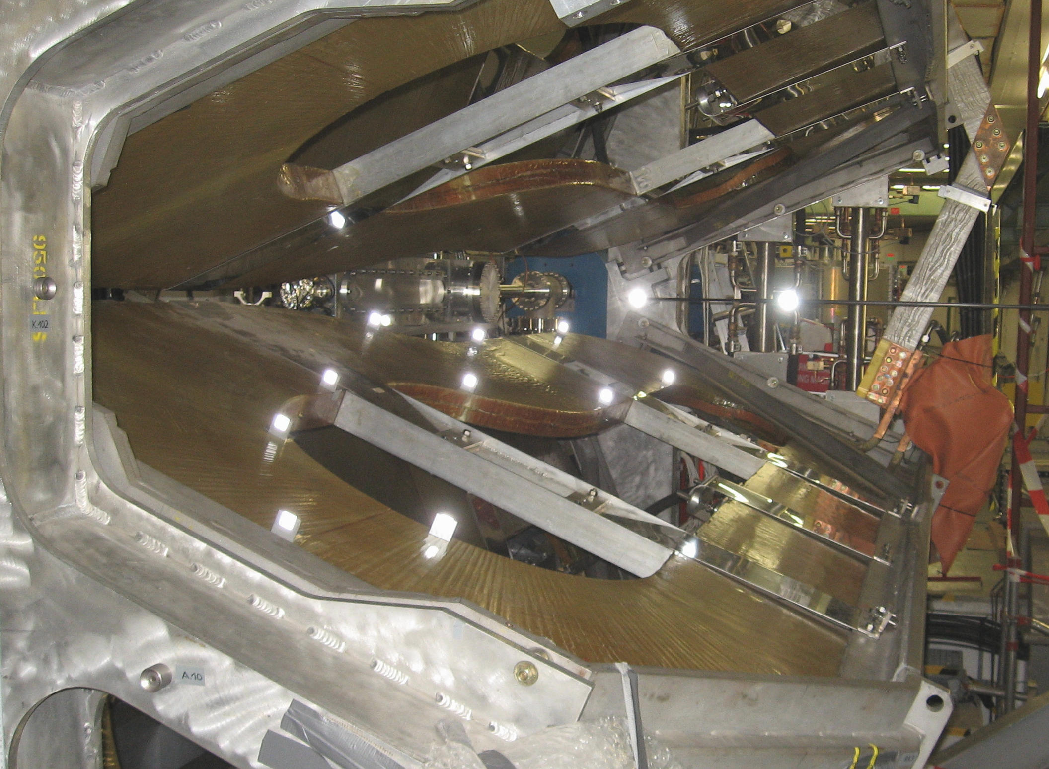
The total station was a really valuable survey tool, since, with its laser tracker, it could determine the coordinates in three dimensions of a target. During the magnetic field measurements, we glued several targets to surfaces of one of the coils, as can been seen in figure B.1. We chose a coil surface that was completely visible to the total station and we arranged the survey targets around the edges of the coil face to bound as much of the coil as possible. We surveyed these targets while the magnet had no current. Then we turned on 5000 A of current and surveyed the targets again. We repeated this procedure several times and tested both magnet polarities. Using the total station’s telescope, it was clear the magnet coil moved from changes in current because the survey targets would leave the cross hairs as the current turned on. Some analysis was needed to determine how much displacement there was.

B.3 Analysis

Figure B.2: Turning on the current caused the coil to move in plane. Most of the motion was towards the beamline, but there was also a slight rotation. The arrows show the displacement magnified by a factor of 100. The largest measured displacement was 2.5 mm.

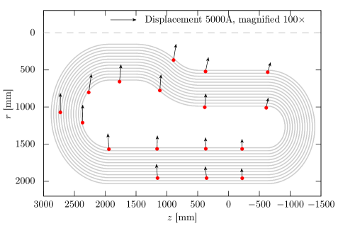
Using the daily calibration data from the total station, we transformed the total station angles and distances into three dimensional positions in the OLYMPUS coordinate system. The results were very clear. When current passed through the magnet, the coils moved by several millimeters. The movement was consistent (to within the $\approx 200~{}\mu$m resolution of the total station) and was the same magnitude and direction regardless of magnet polarity. The motion is almost entirely in the plane of the coil. The in-plane displacements are shown in figure B.2.

B.4 Discussion

Most of the motion appears to be toward the beamline. This was consistent with our expectation. By moving towards the beamline, the coils get closer together, reducing the length of the magnetic field lines. However, it was clear that there was slight rotation of the coils. The wide part of the coil appears displaced farther than the narrow part. This observation lead us to try an in-plane rotation as one of the free parameters when fitting our magnetic field model. In the fit we decided to use (parameters in table 4.1), the in-plane rotation of the upper and lower pair of coils was fit to $0.05^{\circ}$.

Appendix C A Simple Parameterization for Time-to-Distance Functions

C.1 Overview

Figure C.1: We used a simple geometric model to determine the functional dependence on $\alpha$.

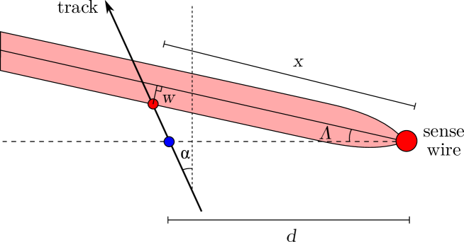
In this appendix, I present the derivation of the simple parameterization for the TTD functions discussed in section 7.5.4. The derivation makes use of a simple two-dimensional geometric model, illustrated in figure C.1. First, I will use the model to derive the approximate dependence on $\alpha$ in the region where the function is linear in $t$. Then I will consider the regions in which the TTD function is no longer linear, when the drift times are very short or very long. Lastly, I will add parameters to allow the function to vary with $\phi$.

In my derivation, I will use the following conventions. The Lorentz angle parameter $\Lambda$ is taken always to be positive. The incidence angle $\alpha$ is 0 when the track is perpendicular to the sense wire plane, positive when the track points further upstream, and negative when the track points further downstream. A track with $\alpha=0$ has a scattering angle of approximately $74^{\circ}$; for most tracks entering the drift chambers $\alpha<0$. I use $\phi$ here to refer to the azimuthal angle from the horizontal plane; that is, a track traveling horizontally left will have $\phi=0^{\circ}$, and a track traveling horizontally right will also have $\phi=0^{\circ}$. This is different from how I use $\phi$ in other chapters, in which a track traveling horizontally to the right has $\phi=180^{\circ}$.

C.2 Linear Region

In the simple geometric model, I assume that the lines of drift form a jet of constant width far from the sense wire, that the jet emerges from the sense wire with an angle $\Lambda$ from the sense wire plane, and that the point at which the first-arriving electrons are ionized is the intersection point of the jet and the track, which sits at approximately distance $x$ from the sense wire. For tracks that intersect the jet in the linear region:

$$d=x\left(\cos\Lambda-\sin\Lambda\tan\alpha\right)+w\left|\sin\Lambda+\cos\Lambda\tan\alpha\right|.$$ (C.1)

To simplify things slightly, I assume $\Lambda$ is always small enough to justify replacing $\sin\Lambda$ with $\Lambda$ and $\cos\Lambda$ with $1$. This leads to:

$$d=x\left(1-\Lambda\tan\alpha\right)+w\left|\Lambda+\tan\alpha\right|.$$ (C.2)

Next, I assume a constant drift velocity $v$ so that $x$ can be replaced with $vt$:

$$d=vt\left(1-\Lambda\tan\alpha\right)+w\left|\Lambda+\tan\alpha\right|.$$ (C.3)

I choose to add an extra parameter, a constant $r$, to allow $d(t)$ to have a non-zero intercept, even when $\Lambda=-\tan\alpha$:

$$d=vt\left(1-\Lambda\tan\alpha\right)+w\left|\Lambda+\tan\alpha\right|+r.$$ (C.4)

The parameter $r$ can be interpreted as a radius around the sense wire in which the ionization electrons cease to drift at a constant velocity and instead accelerate toward the wire.

C.3 Non-linear Regions

Equation C.4 describes a function that is linear in $t$, but captures the non-trivial dependence of $d$ on $\alpha$. This parameterization is suitable for the linear part of the TTD function, between approximately t=0.2 $\mu$s and t=1.1 $\mu$s for most wires (example data are shown in figure 7.10). Special modifications are needed for very small times, where the higher electric fields near the wire increase the drift velocity, and for very large times, where the TTD function plateaus.

For very small times, I choose to approximate the function with a cubic polynomial in $t$. I join the cubic and linear regions at the cut-off point $\psi$ by keeping the first two derivatives continuous:

$$d(t,\alpha)=\begin{dcases}t\left[v\left(1-\Lambda\tan\alpha\right)+\frac{w\left|\Lambda+\tan\alpha\right|+r}{\psi}\left(3-\frac{3t}{\psi}+\frac{t^{2}}{\psi^{2}}\right)\right]&t<\psi,\\ vt\left(1-\Lambda\tan\alpha\right)+w\left|\Lambda+\tan\alpha\right|+r&t\geq\psi.\end{dcases}$$ (C.5)

We typically used a cut-off value $\psi=0.2$ $\mu$s.

For very long times, the TTD function plateaus at a constant value, $d_{\text{max}}$, corresponding to the largest possible drift distance, beyond which the track no longer passes through the active region of the cell. I use the geometric model to determine $d_{\text{max}}$. Given $c$, the distance between the ground plane and the sense wire, then:

$$d_{\text{max}}=c-y\tan\alpha,$$ (C.6)

$$y=\begin{dcases}y_{\text{min}}&\\ \pm\left[c\Lambda-\text{sign}(\alpha)w\right]&\\ y_{\text{max}}&\end{dcases}.$$ (C.7)

The variable $y$ represents the distance between the sense plane and the intersection point of the jet and the ground plane. It has a positive sign for upstream sides of wires on the left sector and downstream sides of wires on the right sector, and otherwise a negative sign. $y$ must be restricted to be within the bounds $[y_{\text{min}},y_{\text{max}}]$, set by the vertical width of the cell: [$-10$ mm, $30$ mm] for inner sense wires, [$-20$ mm, $20$ mm] for middle sense wires, and [$-30$ mm, $10$ mm] for outer sense wires.

By setting $d_{\text{max}}$, I have also set a maximum time:

$$t_{\text{max}}=\frac{d_{\text{max}}-w|\Lambda+\tan\alpha|-r}{v(1-\Lambda\tan\alpha)}.$$ (C.8)

Putting all three regions together, our parameterization becomes:

$$d(t,\alpha)=\begin{dcases}t\left[v\left(1-\Lambda\tan\alpha\right)+\frac{w\left|\Lambda+\tan\alpha\right|+r}{\psi}\left(3-\frac{3t}{\psi}+\frac{t^{2}}{\psi^{2}}\right)\right]&t<\psi,\\ vt\left(1-\Lambda\tan\alpha\right)+w\left|\Lambda+\tan\alpha\right|+r&\psi\leq t<t_{\text{max}},\\ d_{\text{max}}&t_{\text{max}}\leq t.\end{dcases}$$ (C.9)

This parameterization has only four free parameters: $\Lambda$, $w$, $v$, and $r$.

C.4 Adding dependence on $\phi$

So far, this derivation has been entirely two-dimensional; I have not discussed any dependence on $\phi$. Looking at reconstructed tracks, we observe that TTD functions have a weak dependence on $\phi$. In order to allow such a dependence, I make $\Lambda$, $w$, and $v$ quadratic functions of $\phi$:

$$\Lambda \longrightarrow\Lambda_{0}+\Lambda_{1}\phi+\Lambda_{2}\phi^{2},$$ (C.10)

$$w \longrightarrow w_{0}+w_{1}\phi+w_{2}\phi^{2},$$ (C.11)

$$v \longrightarrow v_{0}+v_{1}\phi+v_{2}\phi^{2},$$ (C.12)

raising the total number of free parameters to 10. I choose not to allow $r$ to vary with $\phi$, thinking that if $r$ is determined by the electric field very close to the sense wire, then it should be constant along the length of the wire.

Appendix D An Estimate of the Asymmetry Needed to Resolve the Form Factor Discrepancy

Hard TPE is a possible explanation for the form factor discrepancy. Therefore, in interpreting the results of an asymmetry measurement, one would like to know: is the asymmetry large enough to resolve the discrepancy? In this appendix, I will present a simple way of estimating how much of an asymmetry is needed to fully resolve the form factor discrepancy. My method is by no means the only method for making such an estimate. In fact, you could describe my method as the least sophisticated estimate one can make. I think it is useful for establishing the size scale of the asymmetry and its kinematic dependencies, in the scenario where hard TPE is fully responsible for the discrepancy.

My estimate requires a few assumptions. The first assumption is that the form factor ratio $R\equiv\mu_{p}G_{E}/G_{M}$ as measured by polarization asymmetry experiments describes the true form factor ratio, i.e., the polarization measurements are completely insenstive to hard TPE. Second, I assume that the TPE effect preserves the linearity of Rosenbluth plots. Third, I assume that the TPE effect is zero at $\epsilon=1$. Let’s look at the consequences of these assumptions.

Figure D.1: I assume that hard TPE modifies the slope but preserves the linearity of Rosenbluth plots.

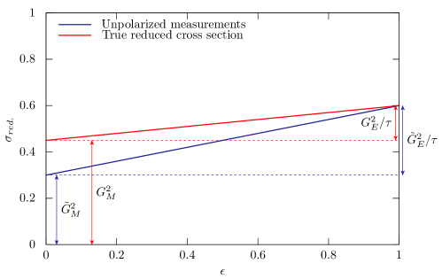
To preserve the linearity of Rosenbluth plots, hard TPE must correct the reduced cross section such that:

$$G_{M}^{2}(Q^{2})+\frac{\epsilon}{\tau}G_{E}^{2}(Q^{2})=\tilde{G}_{M}^{2}(Q^{2})+\frac{\epsilon}{\tau}\tilde{G}_{E}^{2}(Q^{2})+\delta(Q^{2})(1-\epsilon),$$ (D.1)

where $G_{E}$ and $G_{M}$ represent the true form factors, $\tilde{G}_{E}$ and $\tilde{G}_{M}$ represent the form factors extracted from Rosenbluth separation without accounting for hard TPE, and $\delta(Q^{2})$ represents a modification due to hard TPE. The effect of this correction is illustrated in figure D.1. Given the $\epsilon$ dependence of both sides of equation D.1, we find two relationships that must hold at every value of $Q^{2}$:

$$G_{M}^{2} =\tilde{G}_{M}^{2}+\delta$$ (D.2)

$$G_{E}^{2} =\tilde{G}_{E}^{2}-\tau\delta.$$ (D.3)

My first assumption was that the true form factor ratio $R$ can be taken from polarization asymmetry measurements. This leads to:

$$R^{2} =\frac{\mu_{p}^{2}(\tilde{G}_{E}^{2}-\delta\tau)}{\tilde{G}_{M}^{2}+\delta}$$ (D.4)

$$\delta(R^{2}+\tau\mu_{p}^{2}) =\mu_{p}^{2}\tilde{G}_{E}^{2}-R^{2}\tilde{G}_{M}^{2}$$ (D.5)

$$\delta =\frac{\mu_{p}^{2}\tilde{G}_{E}^{2}-R^{2}\tilde{G}_{M}^{2}}{R^{2}+\mu_{p}^{2}\tau}.$$ (D.6)

With an expression for $\delta$ in hand, it is easy to find the size of the asymmetry:

$$A=\frac{\delta(1-\epsilon)}{\tilde{G}_{M}^{2}+\frac{\epsilon}{\tau}\tilde{G}^{2}_{E}+\delta(1-\epsilon)}.$$ (D.7)

To use this method, one must supply $\tilde{G}_{E}$ and $\tilde{G}_{M}$ as taken from Rosenbluth measurements, as well as $R$ as taken from polarization asymmetry measurements, then calculate $\delta$ and $A_{2\gamma}$.

The values of $\tilde{G}_{E}$, $\tilde{G}_{M}$, and $R$ have been measured at several dozen discrete points in $Q^{2}$. To make a prediction as a function of $Q^{2}$, or $\epsilon$, or scattering angle, one must interpolate between the measured data points, or fit some functional form to the data. I will examine the effect of using two such functional forms, one simple, and one sophisticated. For a simple model, I will approximate $\tilde{G}_{E}$, $\tilde{G}_{M}$ as having the standard dipole form. For the sophisticated model, I will use the 2013 Bernauer et al. variable-knot spline fits to cross section data only [57]. As a model for $R$, in both cases, I will use the model:

$$R(Q^{2})=1-(0.12\text{~{}GeV}^{-2})Q^{2},$$

which fits the existing polarization transfer data well enough for our purposes, as can be seen in figure D.2

Figure D.2: Polarization data [22, 23, 24, 25, 26, 27, 28, 29] are well fit by a line with slope 0.12 GeV^-2.

Figure D.3: According to this simple estimate, the lepton sign asymmetry must rise by several percent with decreasing $\epsilon$ in order to resolve the form factor discrepancy. The particular form factors used as input can have a big impact on how large of asymmetry is needed. The discrepancy is bigger if one assumes dipole form factors. If one uses a sophisticated global fit to cross section data [57], the necessary asymmetry is smaller. The uncertainty in the form factor fit introduces uncertainty in how much TPE is needed. Here, I define $1\sigma$ as the uncertainty from statistics and systematics added in quadrature, simply as a rough estimate.

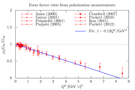
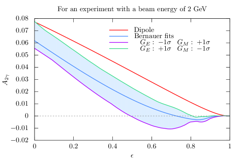
The results of this estimate procedure for both form factor models is shown in figure D.3, for the OLYMPUS beam energy of 2 GeV. These results suggest that the asymmetry should rise to several percent as $\epsilon$ decreases. The choice of form factors can have a big effect on the magnitude of the estimate. Using dipole form factors, the asymmetry needed to resolve the discrepancy rises by nearly 5% over the OLYMPUS acceptance. If one uses a global fit to cross section data, the asymmetry need not be so large. A rise of 3% over the acceptance is sufficient. I have also chosen to show a band corresponding to some measure of the fit uncertainty. This is essentially a measure of how well the form factors are constrained by data, and thus, how well the form factor discrepancy is constrained by data. If the lower error band represents the true form factors, then an asymmetry of less than 2% is sufficient to resolve the discrepancy. I interpret this spread in estimates as a call for caution against making a definite interpretation of the data. An asymmetry that rises to 3% seems suggestive that hard TPE is at play in the form factor discrepancy, but is by no means conclusive.

References

- [1] R. Hofstadter and R. W. McAllister, “Electron Scattering From the Proton,” Phys. Rev., vol. 98, pp. 217–218, 1955.
- [2] R. W. Mcallister and R. Hofstadter, “Elastic Scattering of 188-MeV Electrons From the Proton and the Alpha Particle,” Phys. Rev., vol. 102, pp. 851–856, 1956.
- [3] E. E. Chambers and R. Hofstadter, “Structure of the Proton,” Phys. Rev., vol. 103, pp. 1454–1463, 1956.
- [4] R. W. McAllister, “Absolute Cross Section for Electron Scattering from Protons,” Phys. Rev., vol. 104, pp. 1494–1494, 1956.
- [5] R. Hofstadter, F. Bumiller, and M. R. Yearian, “Electromagnetic structure of the proton and neutron,” Rev. Mod. Phys., vol. 30, pp. 482–497, Apr 1958.
- [6] F. Bumiller, M. Croissiaux, and R. Hofstadter, “Electron Scattering from the Proton,” Phys. Rev. Lett., vol. 5, pp. 261–263, 1960.
- [7] R. Hofstadter, F. Bumiller, and M. Croissiaux, “Splitting of the Proton Form Factors and Diffraction in the Proton,” Phys. Rev. Lett., vol. 5, pp. 263–265, 1960.
- [8] D. Griffiths, Introduction to Elementary Particles. Wiley, 2008.
- [9] M. N. Rosenbluth, “High Energy Elastic Scattering of Electrons on Protons,” Phys. Rev., vol. 79, pp. 615–619, 1950.
- [10] F. Ernst, R. Sachs, and K. Wali, “Electromagnetic form factors of the nucleon,” Phys.Rev., vol. 119, pp. 1105–1114, 1960.
- [11] D. R. Yennie, M. M. Lévy, and D. G. Ravenhall, “Electromagnetic structure of nucleons,” Rev. Mod. Phys., vol. 29, pp. 144–157, Jan 1957.
- [12] L. Andivahis et al., “Measurements of the electric and magnetic form-factors of the proton from to (GeV)2,” Phys. Rev., vol. D50, pp. 5491–5517, 1994.
- [13] K. W. Chen, J. R. Dunning, A. A. Cone, N. F. Ramsey, J. K. Walker, and R. Wilson, “Measurement of Proton Electromagnetic Form Factors at High Momentum Transfers,” Phys. Rev., vol. 141, pp. 1267–1285, 1966.
- [14] T. Janssens, R. Hofstadter, E. B. Hughes, and M. R. Yearian, “Proton form factors from elastic electron-proton scattering,” Phys. Rev., vol. 142, pp. 922–931, 1966.
- [15] W. Bartel, B. Dudelzak, H. Krehbiel, J. M. McElroy, U. Meyer-Berkhout, R. J. Morrison, H. Nguyen-Ngoc, W. Schmidt, and G. Weber, “Small-Angle Electron-Proton Elastic Scattering Cross Sections for Momentum Transfers between 10 and 105 f -2,” Phys. Rev. Lett., vol. 17, pp. 608–611, 1966.
- [16] F. Borkowski, P. Peuser, G. G. Simon, V. H. Walther, and R. D. Wendling, “Electromagnetic Form-Factors of the Proton at Low Four-Momentum Transfer,” Nucl. Phys., vol. B93, pp. 461–478, 1975.
- [17] C. Berger, V. Burkert, G. Knop, B. Langenbeck, and K. Rith, “Electromagnetic form-factors of the proton at squared four momentum transfers between 10 fm-2 and 50 fm-2,” Phys. Lett., vol. B35, pp. 87–89, 1971.
- [18] W. Bartel, F. W. Busser, W. r. Dix, R. Felst, D. Harms, H. Krehbiel, P. E. Kuhlmann, J. McElroy, J. Meyer, and G. Weber, “Measurement of proton and neutron electromagnetic form-factors at squared four momentum transfers up to GeV,” Nucl. Phys., vol. B58, pp. 429–475, 1973.
- [19] R. C. Walker et al., “Measurements of the proton elastic form-factors for (GeV)2 at SLAC,” Phys. Rev., vol. D49, pp. 5671–5689, 1994.
- [20] M. E. Christy et al., “Measurements of electron proton elastic cross-sections for (GeV)2,” Phys. Rev., vol. C70, p. 015206, 2004, nucl-ex/0401030.
- [21] I. A. Qattan et al., “Precision Rosenbluth measurement of the proton elastic form-factors,” Phys. Rev. Lett., vol. 94, p. 142301, 2005, nucl-ex/0410010.
- [22] M. K. Jones et al., “ ratio by polarization transfer in ,” Phys. Rev. Lett., vol. 84, pp. 1398–1402, 2000, nucl-ex/9910005.
- [23] O. Gayou et al., “Measurements of the elastic electromagnetic form-factor ratio via polarization transfer,” Phys. Rev., vol. C64, p. 038202, 2001.
- [24] T. Pospischil et al., “Measurement of via polarization transfer at GeV,” Eur. Phys. J., vol. A12, pp. 125–127, 2001.
- [25] V. Punjabi et al., “Proton elastic form-factor ratios to GeV2 by polarization transfer,” Phys. Rev., vol. C71, p. 055202, 2005, nucl-ex/0501018. [Erratum: Phys. Rev.C71,069902(2005)].
- [26] C. B. Crawford et al., “Measurement of the proton electric to magnetic form factor ratio from vector ,” Phys. Rev. Lett., vol. 98, p. 052301, 2007, nucl-ex/0609007.
- [27] A. J. R. Puckett et al., “Recoil Polarization Measurements of the Proton Electromagnetic Form Factor Ratio to GeV2,” Phys. Rev. Lett., vol. 104, p. 242301, 2010, nucl-ex/1005.3419.
- [28] G. Ron et al., “Low measurements of the proton form factor ratio ,” Phys. Rev., vol. C84, p. 055204, 2011, nucl-ex/1103.5784.
- [29] A. J. R. Puckett et al., “Final Analysis of Proton Form Factor Ratio Data at , and GeV2,” Phys. Rev., vol. C85, p. 045203, 2012, nucl-ex/1102.5737.
- [30] M. Meziane et al., “Search for effects beyond the Born approximation in polarization transfer observables in elastic scattering,” Phys.Rev.Lett., vol. 106, p. 132501, 2011, nucl-ex/1012.0339.
- [31] D. Hasell et al., “The BLAST experiment,” Nucl. Instrum. Meth., vol. A603, pp. 247–262, 2009.
- [32] J. C. Bernauer et al., “Measurement and tricubic interpolation of the magnetic field for the OLYMPUS experiment,” Nucl. Instrum. Meth., vol. A823, pp. 9–14, 2016, physics.ins-det/1603.06510.
- [33] P. A. Guichon and M. Vanderhaeghen, “How to reconcile the Rosenbluth and the polarization transfer method in the measurement of the proton form-factors,” Phys.Rev.Lett., vol. 91, p. 142303, 2003, hep-ph/0306007.
- [34] P. Blunden, W. Melnitchouk, and J. Tjon, “Two-photon exchange and elastic electron-proton scattering,” Phys.Rev.Lett., vol. 91, p. 142304, 2003, nucl-th/0306076.
- [35] M. P. Rekalo and E. Tomasi-Gustafsson, “Model independent properties of two-photon exchange in elastic electron-proton scattering,” Eur.Phys.J., vol. A22, pp. 331–336, 2004, nucl-th/0307066.
- [36] E. Tomasi-Gustafsson and G. Gakh, “Search for evidence of two-photon contribution in elastic electron-proton data,” Phys.Rev., vol. C72, p. 015209, 2005, hep-ph/0412137.
- [37] V. Tvaskis, J. Arrington, M. Christy, R. Ent, C. Keppel, et al., “Experimental constraints on non-linearities induced by two-photon effects in elastic and inelastic Rosenbluth separations,” Phys.Rev., vol. C73, p. 025206, 2006, nucl-ex/0511021.
- [38] Y. C. Chen, C. W. Kao, and S. N. Yang, “Is there model-independent evidence of the two-photon-exchange effect in the electron-proton elastic scattering cross section?,” Phys.Lett., vol. B652, pp. 269–274, 2007, nucl-th/0703017.
- [39] J. Arrington, W. Melnitchouk, and J. Tjon, “Global analysis of proton elastic form factor data with two-photon exchange corrections,” Phys.Rev., vol. C76, p. 035205, 2007, nucl-ex/0707.1861.
- [40] D. Borisyuk and A. Kobushkin, “Phenomenological analysis of two-photon exchange effects in proton form factor measurements,” Phys.Rev., vol. C76, p. 022201, 2007, hep-ph/0703220.
- [41] J. Guttmann, N. Kivel, M. Meziane, and M. Vanderhaeghen, “Determination of two-photon exchange amplitudes from elastic electron-proton scattering data,” Eur.Phys.J., vol. A47, p. 77, 2011, hep-ph/1012.0564.
- [42] D. Borisyuk and A. Kobushkin, “Two-photon exchange amplitudes for the elastic scattering at GeV2 from the experimental data,” Phys.Rev., vol. D83, p. 057501, 2011, hep-ph/1012.3746.
- [43] P. Blunden, W. Melnitchouk, and J. Tjon, “Two-photon exchange in elastic electron-nucleon scattering,” Phys.Rev., vol. C72, p. 034612, 2005, nucl-th/0506039.
- [44] S. Kondratyuk, P. Blunden, W. Melnitchouk, and J. Tjon, “Delta resonance contribution to two-photon exchange in electron-proton scattering,” Phys.Rev.Lett., vol. 95, p. 172503, 2005, nucl-th/0506026.
- [45] S. Kondratyuk and P. Blunden, “Contribution of spin and resonances to two-photon exchange effects in elastic electron-proton scattering,” Phys.Rev., vol. C75, p. 038201, 2007, nucl-th/0701003.
- [46] Y. Chen, A. Afanasev, S. Brodsky, C. Carlson, and M. Vanderhaeghen, “Partonic calculation of the two-photon exchange contribution to elastic electron-proton scattering at large momentum transfer,” Phys.Rev.Lett., vol. 93, p. 122301, 2004, hep-ph/0403058.
- [47] A. V. Afanasev, S. J. Brodsky, C. E. Carlson, Y.-C. Chen, and M. Vanderhaeghen, “The Two-photon exchange contribution to elastic electron-nucleon scattering at large momentum transfer,” Phys.Rev., vol. D72, p. 013008, 2005, hep-ph/0502013.
- [48] D. Borisyuk and A. Kobushkin, “Perturbative QCD predictions for two-photon exchange,” Phys.Rev., vol. D79, p. 034001, 2009, hep-ph/0811.0266.
- [49] N. Kivel and M. Vanderhaeghen, “Two-photon exchange in elastic electron-proton scattering: QCD factorization approach,” Phys.Rev.Lett., vol. 103, p. 092004, 2009, hep-ph/0905.0282.
- [50] N. Kivel and M. Vanderhaeghen, “Two-photon exchange corrections to elastic electron-proton scattering at large momentum transfer within the SCET approach,” JHEP, vol. 1304, p. 029, 2013, hep-ph/1212.0683.
- [51] M. Gorchtein, “Dispersive contributions to e+p/e-p cross section ratio in forward regime,” Phys.Lett., vol. B644, pp. 322–330, 2007, hep-ph/0610378.
- [52] D. Borisyuk and A. Kobushkin, “Box diagram in the elastic electron-proton scattering,” Phys.Rev., vol. C74, p. 065203, 2006, nucl-th/0606030.
- [53] D. Borisyuk and A. Kobushkin, “Two-photon exchange in elastic electron-pion scattering,” Phys.Rev., vol. C83, p. 025203, 2011, hep-ph/1010.4808.
- [54] D. Borisyuk and A. Kobushkin, “On resonance contribution to two-photon exchange amplitude,” Phys.Rev., vol. C86, p. 055204, 2012, hep-ph/1206.0155.
- [55] D. Borisyuk and A. Kobushkin, “Two-photon-exchange amplitude with intermediate states: channel,” Phys.Rev., vol. C89, no. 2, p. 025204, 2014, hep-ph/1306.4951.
- [56] P. Jain, S. D. Joglekar, and S. Mitra, “Two-photon exchange contributions to elastic scattering in the non-local field formalism,” Eur.Phys.J., vol. C52, pp. 339–355, 2007, hep-ph/0606149.
- [57] J. C. Bernauer et al., “Electric and magnetic form factors of the proton,” Phys. Rev., vol. C90, no. 1, p. 015206, 2014, nucl-ex/1307.6227.
- [58] Y. Bystritskiy, E. Kuraev, and E. Tomasi-Gustafsson, “Structure function method applied to polarized and unpolarized electron-proton scattering: A solution of the GE(p)/GM(p) discrepancy,” Phys.Rev., vol. C75, p. 015207, 2007, hep-ph/0603132.
- [59] E. Tomasi-Gustafsson, “On radiative corrections for unpolarized electron-proton elastic scattering,” Phys.Part.Nucl.Lett., vol. 4, pp. 281–288, 2007, hep-ph/0610108.
- [60] C. E. Carlson and M. Vanderhaeghen, “Two-Photon Physics in Hadronic Processes,” Ann.Rev.Nucl.Part.Sci., vol. 57, pp. 171–204, 2007, hep-ph/0701272.
- [61] D. Yount and J. Pine, “Scattering of high-energy positrons from protons,” Phys. Rev., vol. 128, pp. 1842–1849, Nov 1962.
- [62] A. Browman, F. Liu, and C. Schaerf, “Positron-Proton Scattering,” Phys.Rev., vol. 139, pp. B1079–B1085, 1965.
- [63] R. Anderson, B. Borgia, G. Cassiday, J. DeWire, A. Ito, et al., “Scattering of Positrons and Electrons from Protons,” Phys.Rev.Lett., vol. 17, pp. 407–409, 1966.
- [64] W. Bartel, B. Dudelzak, H. Krehbiel, J. McElroy, R. Morrison, W. Schmidt, V. Walther, and G. Weber, “Scattering of positrons and electrons from protons,” Physics Letters B, vol. 25, no. 3, pp. 242 – 245, 1967.
- [65] G. Cassiday, J. DeWire, H. Fischer, A. Ito, E. Loh, and J. Rutherfoord, “Comparison of elastic positron-proton and electron-proton scattering cross sections,” Phys. Rev. Lett., vol. 19, pp. 1191–1192, Nov 1967.
- [66] B. Bouquet, D. Benaksas, B. Grossetête, B. Jean-Marie, G. Parrour, J. Poux, and R. Tchapoutian, “Backward scattering of positrons and electrons on protons,” Physics Letters B, vol. 26, no. 3, pp. 178 – 180, 1968.
- [67] J. Mar, B. C. Barish, J. Pine, D. Coward, H. DeStaebler, et al., “Comparison of electron-proton and positron-proton elastic scattering at four-momentum transfers up to (GeV)2,” Phys.Rev.Lett., vol. 21, pp. 482–484, 1968.
- [68] I. Rachek, J. Arrington, V. Dmitriev, V. Gauzshtein, R. Gerasimov, et al., “Measurement of the two-photon exchange contribution to the elastic scattering cross sections at the VEPP-3 storage ring,” Phys.Rev.Lett., vol. 114, no. 6, p. 062005, 2015, nucl-ex/1411.7372.
- [69] M. Moteabbed et al., “Demonstration of a novel technique to measure two-photon exchange effects in elastic scattering,” Phys. Rev., vol. C88, p. 025210, 2013, nucl-ex/1306.2286.
- [70] D. Adikaram et al., “Towards a resolution of the proton form factor problem: new electron and positron scattering data,” Phys. Rev. Lett., vol. 114, p. 062003, 2015, nucl-ex/1411.6908.
- [71] D. Rimal et al., “Measurement of two-photon exchange effect by comparing elastic cross sections,” 2016, nucl-ex/1603.00315.
- [72] The BLAST Collaboration, “A Proposal for the BATES Large Acceptance Spectrometer Toroid,” report, 1997.
- [73] C. B. Crawford, Precision Measurement of the Proton Electric to Magnetic Form Factor Ratio with BLAST. PhD thesis, Massachusetts Institute of Technology, 2005.
- [74] A. J. Maschinot, Analysis of Scattered Protons in Deuteron Electrodisintegration with a Polarized Electron Beam and an Internal Polarized Target. PhD thesis, Massachusetts Institute of Technology, 2006.
- [75] C. Zhang, Measurement of Tensor Analyzing Powers in Elastic Electron Deuteron Scattering with BLAST. PhD thesis, Massachusetts Institute of Technology, 2006.
- [76] R. Milner, D. Hasell, M. Kohl, U. Schneekloth, N. Akopov, et al., “The OLYMPUS Experiment,” Nuclear Instruments and Methods in Physics Research Section A: Accelerators, Spectrometers, Detectors and Associated Equipment, vol. 741, no. 0, pp. 1–17, 2014, physics.ins-det/1312.1730.
- [77] J. C. Bernauer, V. Carassiti, G. Ciullo, B. S. Henderson, E. Ihloff, J. Kelsey, P. Lenisa, R. Milner, A. Schmidt, and M. Statera, “The OLYMPUS Internal Hydrogen Target,” Nucl. Instrum. Meth., vol. A755, pp. 20–27, 2014, physics.ins-det/1404.0579.
- [78] R. Pérez Benito, D. Khaneft, C. O’Connor, L. Capozza, J. Diefenbach, B. Gläser, Y. Ma, F. Maas, and D. R. Piñeiro, “Design and Performance of a Lead Fluoride Detector as a Luminosity Monitor,” Nucl. Instrum. Meth., vol. A826, pp. 6–14, 2016, physics.ins-det/1602.01702.
- [79] K. A. Dow, T. Botto, A. Goodhue, D. Hasell, D. Loughnan, K. Murphy, T. P. Smith, and V. Ziskin, “Magnetic field measurements of the BLAST spectrometer,” Nucl. Instrum. Meth., vol. A599, pp. 146–151, 2009.
- [80] W. Blum, W. Riegler, and L. Rolandi, Particle Detection with Drift Chambers. Springer, 2008.
- [81] R. L. Russell, A Measurement of the Two-Photon Exchange Effect in Elastic Electron-Proton Scattering with OLYMPUS. PhD thesis, Massachusetts Institute of Technology, Cambridge, Massachusetts, 2016.
- [82] B. S. Henderson, A Precision Measurement of the Elastic Scattering Cross Section Ratio at the OLYMPUS Experiment. PhD thesis, Massachusetts Institute of Technology, Cambridge, Massachusetts, 2016.
- [83] C. O’Connor, The Contribution of Two Photon Exchange in Elastic Lepton-Proton Scattering. PhD thesis, Massachusetts Institute of Technology, Cambridge, Massachusetts, 2017.
- [84] C. O’Connor, “The current olympus solid model for simulation and reconstruction,” Tech. Rep. GDML-006, OLYMPUS internal note, April 2014.
- [85] O. Grimm, J. Rossbach, N. Morozov, A. Chesnov, E. Matyushevsky, D. Petrov, E. Syresin, and Y. Holler, “Magnetic measurements with the FLASH infrared undulator,” 2007.
- [86] F. Lekien and J. Marsden, “Tricubic interpolation in three dimensions,” International Journal for Numerical Methods in Engineering, vol. 63, no. 3, pp. 455–471, 2005.
- [87] P. R. Bevington and D. K. Robinson, Data reduction and error analysis for the physical sciences; 3rd ed. New York, NY: McGraw-Hill, 2003.
- [88] J. S. Schwinger, “Quantum electrodynamics. III: The electromagnetic properties of the electron: Radiative corrections to scattering,” Phys.Rev., vol. 76, pp. 790–817, 1949.
- [89] L. W. Mo and Y.-S. Tsai, “Radiative corrections to elastic and inelastic and scattering,” Rev. Mod. Phys., vol. 41, pp. 205–235, Jan 1969.
- [90] Y.-S. Tsai, “Radiative corrections to electron-proton scattering,” Phys. Rev., vol. 122, pp. 1898–1907, Jun 1961.
- [91] N. Meister and D. R. Yennie, “Radiative corrections to high-energy scattering processes,” Phys. Rev., vol. 130, pp. 1210–1229, May 1963.
- [92] L. C. Maximon and J. A. Tjon, “Radiative corrections to electron-proton scattering,” Phys. Rev. C, vol. 62, p. 054320, Oct 2000, nucl-th/0002058.
- [93] R. Ent, B. W. Filippone, N. C. R. Makins, R. G. Milner, T. G. O’Neill, and D. A. Wasson, “Radiative corrections for reactions at GeV energies,” Phys. Rev. C, vol. 64, p. 054610, Oct 2001.
- [94] D. R. Yennie, S. C. Frautschi, and H. Suura, “The infrared divergence phenomena and high-energy processes,” Annals Phys., vol. 13, pp. 379–452, 1961.
- [95] A. V. Gramolin, V. S. Fadin, A. L. Feldman, R. E. Gerasimov, D. M. Nikolenko, I. A. Rachek, and D. K. Toporkov, “A new event generator for the elastic scattering of charged leptons on protons,” J. Phys., vol. G41, no. 11, p. 115001, 2014, nucl-ex/1401.2959.
- [96] J. C. Bernauer, Measurement of the elastic electron-proton cross section and separation of the electric and magnetic form factor in the range from to (GeV/)2. PhD thesis, Johannes Gutenberg-Universitä t Mainz, Mainz, Germany, 2010.
- [97] J. J. Kelly, “Simple parametrization of nucleon form factors,” Phys. Rev., vol. C70, p. 068202, 2004.
- [98] F. Ignatov, “Vacuum polarization.” http://cmd.inp.nsk.su/~ignatov/vpl/. Accessed: 2016-05-23.
- [99] F. Ignatov, “Calculation of the vacuum polarization,” The 4th Meeting of the Working Group on Rad. Corrections and MC Generators for Low Energies, IHEP, Beijing, 2008.
- [100] C. S. Epstein and R. G. Milner, “QED radiative corrections to low-energy Møller and Bhabha scattering,” Phys. Rev., vol. D94, no. 3, p. 033004, 2016, nucl-ex/1602.07609.
- [101] A. Schmidt and J. Bernauer, “The comparator saturation hypothesis: how this explains what we see, and what it means for the symbs,” Tech. Rep. SM-000, OLYMPUS internal note, May 2016.
- [102] M. Dell’Orso and L. Ristori, “A Highly parallel algorithm for track finding,” Nucl. Instrum. Meth., vol. A287, pp. 436–438, 1990.
- [103] M. Ohlsson, C. Peterson, and A. L. Yuille, “Track finding with deformable templates: The Elastic arms approach,” Comput. Phys. Commun., vol. 71, pp. 77–98, 1992.
- [104] M. Ohlsson, “Extensions and explorations of the elastic arms algorithm,” Comput. Phys. Commun., vol. 77, pp. 19–32, 1993.
- [105] M. Lindstrom, “Track reconstruction in the ATLAS detector using elastic arms,” Nucl. Instrum. Meth., vol. A357, pp. 129–149, 1995.
- [106] “Garfield—simulation of tracking detectors.” http://garfieldpp.web.cern.ch/garfieldpp/. Accessed: 2016-08-23.
- [107] “Magboltz—transport of electrons in gas mixtures.” http://magboltz.web.cern.ch/magboltz/. Accessed: 2016-08-23.
- [108] S. Agostinelli et al., “GEANT4: A Simulation toolkit,” Nucl. Instrum. Meth., vol. A506, pp. 250–303, 2003.
- [109] L. D. Ice, Measuring the Two-Photon Exchange Contribution to Lepton-Proton Scattering with OLYMPUS. PhD thesis, Arizona State University, Tempe, Arizona, 2016.