Accelerated Optimization in the PDE Framework:
Formulations for the Active Contour Case

Following the seminal work of Nesterov, accelerated optimization methods have been used to powerfully boost the performance of first-order, gradient-based parameter estimation in scenarios where second-order optimization strategies are either inapplicable or impractical. Not only does accelerated gradient descent converge considerably faster than traditional gradient descent, but it also performs a more robust local search of the parameter space by initially overshooting and then oscillating back as it settles into a final configuration, thereby selecting only local minimizers with a basis of attraction large enough to contain the initial overshoot. This behavior has made accelerated and stochastic gradient search methods particularly popular within the machine learning community. In their recent PNAS 2016 paper, Wibisono, Wilson, and Jordan demonstrate how a broad class of accelerated schemes can be cast in a variational framework formulated around the Bregman divergence, leading to continuum limit ODE’s. We show how their formulation may be further extended to infinite dimension manifolds (starting here with the geometric space of curves and surfaces) by substituting the Bregman divergence with inner products on the tangent space and explicitly introducing a distributed mass model which evolves in conjunction with the object of interest during the optimization process. The co-evolving mass model, which is introduced purely for the sake of endowing the optimization with helpful dynamics, also links the resulting class of accelerated PDE based optimization schemes to fluid dynamical formulations of optimal mass transport.

1 Introduction

Following the seminal work of Nesterov, accelerated optimization methods (sometimes referred to as momentum methods) have been used to powerfully boost the performance of first-order, gradient-based parameter estimation in scenarios where second-order optimization strategies are either inapplicable or impractical. Not only does accelerated gradient descent converge considerably faster than traditional gradient descent, but it also performs a more robust local search of the parameter space by initially overshooting and then oscillating back as it settles into a final configuration, thereby selecting only local minimizers with a basis of attraction large enough to contain the initial overshoot. This behavior has made accelerated and stochastic gradient search methods particularly popular within the machine learning community [29, 26, 25, 21, 20, 19, 15, 14, 5, 40]. So far, however, accelerated optimization methods have been restricted to searches over finite dimensional parameter spaces.

Recently, however, Wibisono, Wilson, and Jordan outlined a variational ODE framework in [54] (which we will summarize briefly in Section 2.4) formulated around the Bregman divergence and which yields the continuum limit of a broad class of accelerated optimization schemes, including that of Nesterov’s accelerated gradient method [30] whose continuum ODE limit was also demonstrated by Su, Boyd, and Candes in [46]. Here he will show how a similar high level framework may be adapted for infinite dimensional manifolds through the formulation of a generalized time-explicit action which can be viewed both as a specialization and generalization of the Bregman Lagrangian presented in [54]. While the extension we outline from the ODE framework into the PDE framework is general enough to be applied to a variety of infinite-dimensional or distributed-parameter optimization problems (dense shape reconstruction/inversion, optical flow estimation, image restoration, etc.) the specific examples presented here will focus on the active contour and active surface based optimization.

Moving into the infinite dimensional framework introduces additional mathematical, numerical, and computational challenges and technicalities which do not arise in finite dimensions. For example, the evolving parameter vector in finite dimensional optimization can naturally be interpreted as a single moving particle in $\mathbf{R}^{n}$ with a constant mass which, in accelerated optimization schemes, gains momentum during its evolution. Since the mass is constant and fixed to a single particle, there is no need to explicitly model it. When evolving a continuous curve, surface, region, or function, however, the notion of accumulated momentum during the acceleration process is much more flexible, as the corresponding conceptual mass can be locally distributed in several different ways throughout the domain which will in turn significantly affect the evolution dynamics. In fact we intend to exploit this added design flexibility to further capture some of the same coarse-to-fine regularization properties of Sobolev gradient flows [55, 47] within the accelerated optimization context as well, but with far less computational cost.

The discrete implementation of accelerated PDE models will also differ greatly from existing momentum based gradient descent schemes in finite dimensions. Spatial and temporal steps sizes will be determined based on CFL stability conditions for finite difference approximations of the PDE’s. Finally, in the PDE framework, viscosity solutions will be required in most cases to propagate through shocks and rarefactions that may occur during the evolution of a continuous front, a phenomenon which manifests itself differently and is therefore handled differently in the finite dimensional case. As such, these considerations will also impact the numerical discretization of accelerated PDE models.

Finally, in part due to these different discretization criteria and in part to avoid unnecessary complexity in the manifold case, we will abandon the Bregman Lagrangian described in [54] and will instead exploit a simpler time-explicit generalized action which will allow us to work directly with the continuum velocity of the evolving entity rather than finite displacements with the Bregman divergence. Especially for the case of curves and surfaces considered here, this avoids the complication of calculating geodesic distances on highly curved, infinite-dimensional manifolds, but lets us work more easily in the tangent space instead.

2 Background and Prior Work

Geometric partial differential equations have played an important role in image analysis and computer vision for several decades now. Applications have ranged from low-level processing operations such as denoising using anisotropic diffusion, blind deconvolution, and contrast enhancement; to mid-level processing such as segmentation using active contours and active surfaces, image registration, and motion estimation via optical flow; to higher level processing such as multiview stereo reconstruction, visual tracking, SLAM, and shape analysis. See, for example, [45, 44, 41] for introductions to PDE methods already established within computer vision within the 1990’s, including level set methods [42] already developed in the 1980’s for shape propagation. Several such PDE methods have been formulated, using the calculus of variations [52] as gradient descent based optimization problems in functional spaces, including geometric spaces of curves and surfaces.

During the past decade a popular trend has arisen whereby several such variational problems, which are non-convex, have been reformulated and relaxed to convex optimization problems [9, 7, 17, 43], which allows one to build on the wealth of algorithms developed in the optimization literature [4]. While such methods have led to efficient and robust numerical schemes, the class of problems for which such reformulations apply are a limited class. We seek to develop optimization methods for a wider class of (non-convex) problems.

Recently, Chaudhari et. al. have established connections between relaxation techniques used in training deep neural networks, and PDE’s in [12] based on the continuum Fokker-Planck equation limit. They, in turn, develop and demonstrate improved implementations of stochastic gradient descent based on the viscous Hamilton-Jacobi equation. Subsequently, in [13], Chaudhari and Soatto demonstrate that stochastic gradient descent (SGD) methods perform variational inference (although not on the original loss function). While they do exploit momentum to accelerate convergence in their numerical algorithms, this acceleration component is introduced on the backend of the final discreet algorithm. The methodology presented in Section 3.2.3, through the incorporation of an auxiliary evolving density function, offers a potential strategy to directly integrate acceleration into their original continuum PDE formulation of SDG as well. However, our focus here will remain exclusively on acceleration, by itself, within the continuum PDE framework.

2.1 Geometric Active Contours (an example of gradient PDE optimization)

For example, several active contour models are formulated as gradient descent PDE flows of application-specific energy functionals $E$ which relate the unknown contour $C$ to given data measurements. Such energy functionals are chosen to depend only upon the geometric shape of the contour $C$, not its parameterization. Under these assumptions the first variation of $E$ will have the following form

$$\delta E =-\int_{C}f\,(\delta C\cdot N)\,ds$$ (1)

where $fN$ represents a perturbation field along the unit normal $N$ at each contour point and $ds$ denotes the arclength measure. Note that the first variation depends only upon the normal component of a permissible contour perturbation $\delta C$. The form of $f$ will depend upon the particular choice of the energy. For example, in the popular Chan-Vese active contour model [8] for image segmentation, $f$ would be expressed by $(I-c_{1})^{2}-(I-c_{2})^{2}+\alpha\kappa$ where $I$ denotes the image value at a given contour point, $\alpha$ an arclength penalty weight, $\kappa$ the curvature at a given contour point, and $c_{1}$ and $c_{2}$ the means of the image inside and outside the contour respectively. As an alternative example, the geodesic active contour model [6, 24] would correspond to $f=\phi\kappa N-(\nabla\phi\cdot N)N$ where $\phi>0$ represents a point measurement designed to be small near a boundary of interest and large otherwise. In all cases, though, the gradient descent PDE will the following explicit form.

$$\frac{\partial C}{\partial t}=fN\quad\mbox{[explicit gradient flow]}$$ (2)

This class of contour flows, evolving purely in the normal direction, may be implemented implicitly in the level set framework [42] by evolving a function $\psi$ whose zero level set represents the curve $C$ as follows

$$\frac{\partial\psi}{\partial t}=-\hat{f}\|\nabla\psi\|\quad\mbox{[implicit level set flow]}$$

where $\hat{f}(x,t)$ denotes a spatial extension of $f(s,t)$ to points away from the curve.

2.2 Sobolev gradients for more robust coarse-to-fine PDE based optimization

The most notorious problem with most active contour and active surface models is that the normal speed function $f$ depends pointwise upon noisy or irregular data measurements, causing immediate fine scale perturbations in the evolving contour which cause it to become very easily attracted to (and trapped within) spurious local minimizers. This often makes the active contour model strongly dependent upon initialization, except for a limited class of convex or poly-convex energy functionals for which numerical schemes can be devised to reach global minimzers reliably. The traditional way to combat this sensitivity is to add strong regularizing terms to the energy functional which penalize fine scale irregularities in the contour shape. Similar problems and regularization strategies are applied in other PDE based optimization applications outside the realm of the illustrative active contour example being considered here (for example, in Horn and Schunck style optical flow computation [18]).

This energy regularization strategy has two drawbacks. First, most regularizers lead to second order (or higher) diffusion terms in the gradient contour flow, which impose much smaller time step limitations on the numerical discretization of the evolution PDE. Thus, significantly more evolution steps are required, which incurs a heavy computational cost in the minimization process. Second, regularizers, while endowing a level of resistance to noise and spurious structure, impose regularity on the final converged contour as well, making it difficult or impossible to capture features such as sharp corners, or narrow protrusions/inlets in the detected shape. This can lead to unpleasant trade-offs in several applications.

For the illustrative case of active contours, significantly improved robustness in the gradient flow, without additional energy regularization, can be attained by using geometric Sobolev gradients [10, 11][50, 51] in place of the standard $L^{2}$-style gradient used in traditional active contours. We refer to this class of active contours as Sobolev active contours, whose evolution may be described by the following integral-partial-differential equation

$$\frac{\partial C}{\partial t}=\left(fN\right)\ast K\quad\mbox{[Sobolev gradient flow]}$$ (3)

Here $\ast$ denotes convolution in the arclength measure with a smoothing kernel $K$ to invert the linear Sobolev gradient operator. The numerical implementation is not carried out this way, but the expression gives helpful insight into how the Sobolev gradient flow (3) relates to the usual gradient flow (2). Namely, the optimization process (rather than the energy functional itself) is regularized by averaging point-wise gradient forces $fN$ through the kernel $K$ to yield a smoother contour evolution. This does not change the local minimizers of the energy functional, nor does it impose extra regularity at convergence, but it induces a coarse-to-fine evolution behavior [47, 55] in the contour evolution, making it much more resistant to spurious local minima due to noise or other fluctuations in $f$.

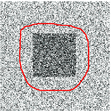
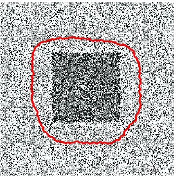
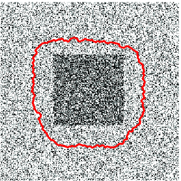
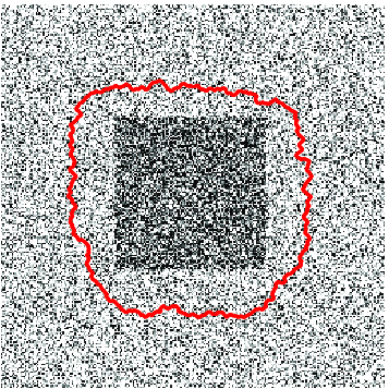
Active contour (evolving left-to-right) without regularization
Active contour (evolving left-to-right) with added regularization
Sobolev active contour (evolving left-to-right) without regularization

Figure 1: Sobolev gradients versus energy regularization

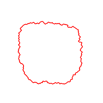
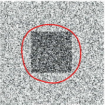
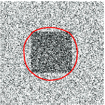
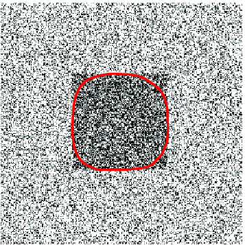
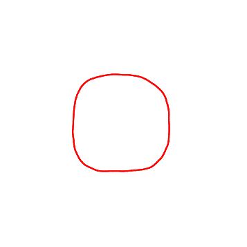
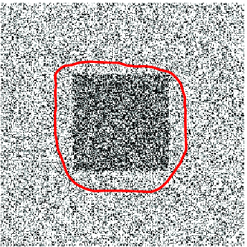
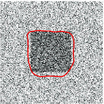
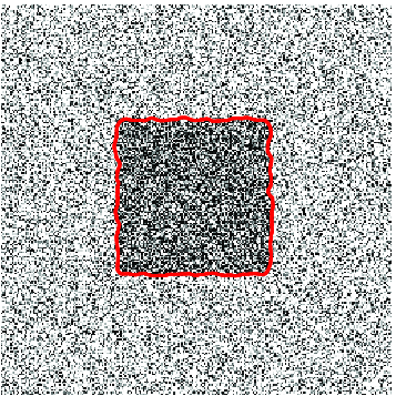
The regularity of the coarse-to-fine Sobolev gradient flow compared with regularity imposed on the energy functional is illustrated in Figure 1. Along the top row we see the evolution of a standard active contour in a very noisy image without regularizing terms in the energy function to keep the contour smooth. The contour quickly gets trapped in a noisy local minimum configuration before reaching the desired square boundary. Of course, we can add a regularizing term to the energy to prefer smoother contours. We see in the middle row (b) that this fixes the noise problem but does not allow us to capture the sharp corners of the square. Along the bottom row, instead, we show the evolution of the Sobolev active contour for the original unregularized energy from the top row. The initial stages of the evolution maintain a smooth contour, not because the Sobolev gradient prefers a smooth contour, but because it prefers a smooth evolution. As the Sobolev active contour nears the boundary of the square, finer scale motions are incorporated to bring out the corners. The final converged contour responds to local noise, but only in the vicinity of a desired minimizer.

However, while the Sobolev gradient descent method is extremely successful in making an active contour or surface (or other evolving classes of functions) resistant to a large class of unwanted local minimizers, it comes at heavy computation cost. The spatial integration of gradient forces along the evolving front must occur during every time step, and while there are tricks to do this quickly for closed 2D curves [27, 49, 48, 2] there are no convenient alternatives for 3D surfaces, nor for regions (even in 2D) when applying Sobolev gradient flows to other functional objects (images, optical flow, etc.). The linear operator inversion imposes a notable per-iteration cost, which we will instead distribute across iterations in the upcoming accelerated coupled PDE evolution schemes.

2.3 Momentum methods and Nesterov’s Accelerated Gradient

If we step back to the finite dimensional case, an alternative and computationally cheaper method to regularize any gradient descent based iteration scheme is to employ the use of momentum. In such schemes the new update becomes a weighted combination of the previous update (the momentum term) and the newly computed gradient at each step. This leads to a temporal averaging of gradient information computed and accumulated during the evolution process itself, rather than a spatial averaging that occurs independently during each time step. As such it adds insignificant per-iteration computation cost while significantly boosting the robustness (and often the convergence speed) of the optimization process.

Momentum methods, including stochastic variants [15, 19], have become very popular in machine learning in recent years [5, 14, 20, 21, 25, 29, 40, 26]. Strategic dynamically changing weights on the momentum term can further boost the descent rate. Nesterov put forth the following famous scheme [30] which attains an optimal rate of order $\frac{1}{t^{2}}$ in the case of a smooth, convex energy function $E(x)$

$$y_{k+1}=x_{k}-\frac{1}{\beta}\nabla E(x_{k}),\qquad x_{k+1}=(1-\gamma_{k})y_{k+1}+\gamma_{k}y_{k},\qquad\gamma_{k}=\frac{1-\lambda_{k}}{\lambda_{k}+1},\qquad\lambda_{k}=\frac{1+\sqrt{1+4\lambda_{k-1}^{2}}}{2}$$

where $x_{k}$ is the $k$-th iterate of the algorithm, $y_{k}$ is an intermediate sequence, and $\gamma_{k}$ are dynamically updated weights.

2.4 A Variational Framework for Accelerated ODE Optimization

Recently in [54] Wibisono, Wilson, and Jordan presented a variational generalization of Nesterov’s [30] and other momentum based gradient descent schemes in $\mathbb{R}^{n}$ based on the Bregman divergence of a convex distance generating function $h$

$$D(y,x)=h(y)-h(x)-\left\langle\nabla h(x),y-x\right\rangle$$ (4)

and careful discretizations of the Euler-Lagrange equation for the time integral (evolution time) of the following Bregman Lagrangian

$${\cal L}(X,V,t)=e^{a(t)+\gamma(t)}\left[D(X+e^{-a(t)}V,X)-e^{b(t)}{\bf U}(X)\right]$$

where the potential energy ${\bf U}$ represents the cost to be minimized. In the Euclidean case, where $D(y,x)=\frac{1}{2}\|y-x\|^{2}$, this simplifies to

$${\cal L}=e^{\gamma(t)}\left[e^{-a(t)}\underbrace{\frac{1}{2}\|V\|^{2}}_{{\bf T}}-e^{a(t)+b(t)}{\bf U}(X)\right]$$

where ${\bf T}$ models the kinetic energy of a unit mass particle in $\mathbb{R}^{n}$. Nesterov’s methods [30, 34, 33, 32, 35, 31] belong to a subfamily of Bregman Lagrangians with the following choice of parameters (indexed by $k>0$)

$$a=\log k-\log t,\qquad b=k\,\log t+\log\lambda,\qquad\gamma=k\,\log t$$

which, in the Euclidean case, yields a time-explicit generalized action (compared to the time-implicit standard action ${\bf T}-{\bf U}$ from classical mechanics [16]) as follows.

$${\cal L}=\frac{t^{k+1}}{k}\left({\bf T}-\lambda k^{2}t^{k-2}{\bf U}\right)$$ (5)

In the case of $k=2$, for example, the Euler-Lagrange equations for the integral of this time-explicit action yield the continuum limit of Nesterov’s accelerated mirror descent[31] derived in both [46, 25].

3 Accelerated Optimization in the PDE Framework

We now develop a general strategy, based on a generalization of the Euclidean case of Wibisono, Wilson, and Jordan’s formulation [54] reviewed in Section 2.4, for extending accelerated optimization into the PDE framework. While our approach will be motivated by the variational ODE framework formulated around the Bregman divergence in [54], we will have to address several mathematical, numerical, and computational considerations which do not need to be addressed in finite dimenions.

For example, the evolving parameter vector in finite dimensional optimization can naturally be interpreted as a single moving particle in $\mathbf{R}^{n}$ with a constant mass which, in accelerated optimization schemes, gains momentum during its evolution. Since the mass is constant and fixed to a single particle, there is no need to explicitly model it. When evolving a continuous curve, surface, region, or function, however, the notion of accumulated momentum during the acceleration process is much more flexible, as the corresponding conceptual mass can be locally distributed in several different ways throughout the domain which will in turn significantly affect the evolution dynamics. We outline two different mass models in Sections 3.2.2 and 3.2.3 as starting points and show how additional control of the optimization dynamics can be introduced in conjunction with the more flexible second mass model by considering independent mass-related potential energy terms in Section 3.5.2. In all cases, the outcome of these formulations will be a coupled system of first-order PDE’s which govern the simultaneous evolution of the continuous unknown (curves in the case considered here), its velocity, as well as the supplementary density function which describes the evolving mass.

In addition, as pointed out from the onset, the numerical discretization of accelerated PDE models will also differ greatly from existing momentum based gradient descent schemes in finite dimensions. Spatial and temporal steps sizes will be determined based on CFL stability conditions for finite difference approximations of the PDE’s and viscosity solution schemes will be required in most cases to propagate through shocks and rarefactions that may occur during the evolution of a continuous front. This is part of the reason we replace the more general Bregman-Lagrangian in [54] with the simpler time-explicit generalized action (5), together with the additional benefit that such a choice allows us to work directly with the continuum velocity of the evolving entity (or other generalizations that are easily defined within the tangent space of its relevant manifold) rather than finite displacements utilized by the Bregman divergence (4).

3.1 General Approach

Just as in [54], the energy functional $E$ to be optimized over the continuous infinite dimensional unknown (whether it be a function, a curve, a surface, or a diffeomorphic mapping) will represent the potential energy term ${\bf U}$ in the time-explicit generalized action (5). Next, a customized kinetic energy term ${\bf T}$ will be formulated to incorporate the dynamics of the evolving estimate during the minimization process. Note that just as the evolution time $t$ would represent an artificial time parameter for a continuous gradient descent process, the kinetic energy term will be linked to artificial dynamics incorporated into the accelerated optimization process. As such, the accelerated optimization dynamics can be designed completely independently of any potential physical dynamics in cases where the unknown might be connected with the motion of real objects. Several different strategies can be explored, depending upon the geometry of the specific optimization problem, for defining kinetic energy terms, including various approaches for attributing artificial mass (both its distribution and its flow) to the actual unknown of interest in order to boost the robustness and speed of the optimization process.

Figure 2: Accelerated descent physics interpretation

Once the kinetic energy term has been formulated, the accelerated evolution will obtained (prior to discretization) using the Calculus of Variations[52] as the Euler-Lagrange equation of the following time-explicit generalized action integral

$$\int\frac{t^{k+1}}{k}\left({\bf T}-\lambda k^{2}t^{k-2}{\bf U}\right)\,dt$$ (6)

In the simple $k=2$ case, the main difference between the resulting evolution equations versus the classical Principle of Least Action equations of motion (without the time explicit terms in the Lagrangian) is an additional friction-style term whose coefficient of friction decreases inversely proportional to time. This additional term, however, is crucial to the accelerated minimization scheme. Without such a frictional term, the Hamiltonian of the system (the total energy ${\bf T}+{\bf U}$), would be conserved, and the associated dynamical evolution would never converge to a stationary point. Friction guarantees a monotonic dissipation of energy, allowing the evolution to converge to a state of zero kinetic energy and locally minimal potential energy (the optimization objective).

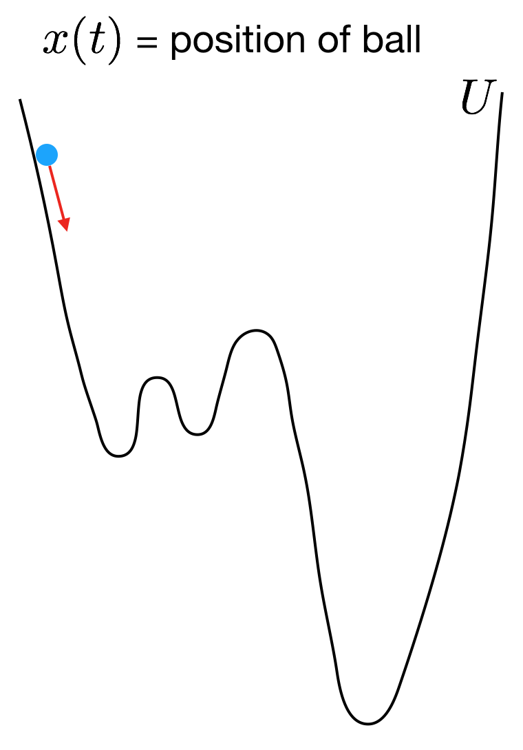
This yields a natural physical interpretation of accelerated gradient optimization in terms of a mass rolling down a potentially complicated terrain by the pull of gravity (Figure 2). In gradient descent, its mass is irrelevant, and the ball always rolls downward by gravity (the gradient). As such the gradient directly regulates its velocity. In the accelerated case, gravity regulates its acceleration. Friction can be used to interpolate these behaviors, with gradient descent representing the infinite frictional limit as pointed out in [54].

Acceleration comes with two advantages. First, whenever the gradient is very shallow (the energy functional is nearly flat), acceleration allows the ball to accumulate velocity as it moves so long as the gradient direction is self reinforcing. As such, the ball approaches a minimum more quickly. Second, the velocity cannot abruptly change near a shallow minimum as in gradient descent. Its mass gives it momentum, and even if the acceleration direction switches in the vicinity of a shallow minimum, the accumulated momentum still moves it forward for a certain amount of time, allowing the optimization process to look ahead for a potentially deeper minimizer.

3.2 Accelerated Active Contours

We now illustrate the steps in the process for developing PDE based accelerated optimization schemes for the specific case of geometric active contours. The resulting coupled PDE evolutions will retain the parameterization independent property of gradient descent based active contours models and will therefore remain amenable to implicit implementation using Level Set Methods [42].

We begin, however, by reviewing some basic differential contour evolution properties that will be useful in deriving accelerated active contour formulations. In particular, it is useful to understand any contour evolution behavior in terms of its local geometric frame, consisting of the unit tangent and normal vectors.

Let $C(p,t)$ denote an evolving curve where $t$ represents the evolution parameter and $p\in[0,1]$ denotes an independent parameter along each fixed curve. The unit tangent, unit normal, and curvature will be denoted by $T=\frac{\partial C}{\partial s}$, $N$, and $\kappa$ respectively, with the sign convention for $\kappa$ and the direction convention for $N$ chosen to respect the planar Frenet equations $\frac{\partial T}{\partial s}=\kappa N$ and $\frac{\partial N}{\partial s}=-\kappa T$, where $s$ denotes the time-dependent arclength parameter whose derivative with respect to $p$ yields the parameterization speed $\frac{\partial s}{\partial p}=\left\|\frac{\partial C}{\partial p}\right\|$.

Letting $\alpha$ and $\beta$ denote the tangential and normal speeds of the evolving curve,

$$\frac{\partial C}{\partial t}=\alpha T+\beta N$$ (7)

the frame itself can be shown to evolve as follows.

$$\frac{\partial T}{\partial t}=\left(\frac{\partial\beta}{\partial s}+\alpha\kappa\right)\,N,\qquad\frac{\partial N}{\partial t}=-\left(\frac{\partial\beta}{\partial s}+\alpha\kappa\right)\,T$$ (8)

Differentiating the velocity decomposition (7) with respect to $t$, followed by the frame evolution (8) substitution, yields the acceleration

$$\frac{\partial^{2}C}{\partial t^{2}}=\left(\frac{\partial\alpha}{\partial t}-\beta\left(\frac{\partial\beta}{\partial s}+\alpha\kappa\right)\right)\,T+\left(\frac{\partial\beta}{\partial t}+\alpha\left(\frac{\partial\beta}{\partial s}+\alpha\kappa\right)\right)\,N$$ (9)

which may be rewritten as the following two scalar evolution equations for the tangential and normal speeds, in terms of the tangential and normal components of the contour acceleration, respectively.

$$\frac{\partial\alpha}{\partial t}=\frac{\partial^{2}C}{\partial t^{2}}\cdot T+\beta\left(\frac{\partial\beta}{\partial s}+\alpha\kappa\right),\qquad\frac{\partial\beta}{\partial t}=\frac{\partial^{2}C}{\partial t^{2}}\cdot N-\alpha\left(\frac{\partial\beta}{\partial s}+\alpha\kappa\right)$$ (10)

3.2.1 Contour potential energy

For geometric active contours, we start by defining the potential energy ${\bf U}$ to be an originally provided energy functional $E$ which depends only upon the geometric shape of the contour $C$ (not its parameterization). Under these assumptions the first variation of the potential energy will have the following form, just as in (1) presented earlier in Section 2.1, where $fN$ denotes the backward local gradient force at each contour point.

$$\delta{\bf U} =-\int_{C}f\,(\delta C\cdot N)\,ds$$

3.2.2 Constant density model

To formulate an accelerated evolution model, we define a kinetic energy, which requires a notion of mass coupled with velocity. The simplest starting model would be one of constant mass density $\rho$ (per unit arclength along the contour) and an integral of the squared norm of the point-wise contour evolution velocity.

$${\bf T}=\frac{1}{2}\rho\int_{C}\left(\frac{\partial C}{\partial t}\cdot\frac{\partial C}{\partial t}\right)ds$$ (11)

Plugging this into the generalized action integral (6) and computing the Euler-Lagrange equation leads to our first, and simplest, accelerated model.

$$\underbrace{\frac{\partial^{2}C}{\partial t^{2}}}_{\mbox{acceleration}}=\frac{\lambda k^{2}t^{k-2}}{\rho}\underbrace{fN}_{-\mbox{gradient}}-\underbrace{\left(\frac{\partial^{2}C}{\partial s\partial t}\cdot\frac{\partial C}{\partial s}\right)\frac{\partial C}{\partial t}-\frac{\partial}{\partial s}\left(\frac{1}{2}\left\|\frac{\partial C}{\partial t}\right\|^{2}\frac{\partial C}{\partial s}\right)}_{\mbox{wave propagation terms}}-\underbrace{\frac{k+1}{t}\frac{\partial C}{\partial t}}_{\mbox{friction}}$$ (12)

If we start with zero initial velocity we can decompose this nonlinear second-order PDE into the following coupled system of nonlinear first order PDE’s

$$\frac{\partial C}{\partial t}=\beta N,\qquad\frac{\partial\beta}{\partial t}=\frac{\lambda k^{2}t^{k-2}}{\rho}f+\frac{1}{2}\beta^{2}\kappa-\frac{k+1}{t}\beta$$ (13)

Since the contour evolution remains purely geometric (only in the normal direction $N$) we may also write down an implicit level set version of the coupled PDE system as follows

$$\frac{\partial\psi}{\partial t}=\hat{\beta}\|\nabla\psi\|,\qquad\frac{\partial\hat{\beta}}{\partial t}=\frac{\lambda k^{2}t^{(k-2)}}{\rho}\hat{f}+\nabla\cdot\left(\frac{1}{2}\hat{\beta}^{2}\frac{\nabla\psi}{\|\nabla\psi\|}\right)-\frac{k+1}{t}\hat{\beta}$$ (14)

where $\hat{f}(x,t)$ and $\hat{\beta}(x,t)$ denote spatial extensions of $f$ and $\beta$ respectively.

Illustrative results

Figure 3: Three active contours getting stuck in different local minima

Figure 4: Accelerated active contours all converging to same minimzer

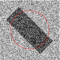
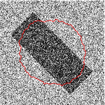
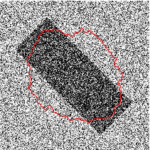
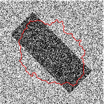
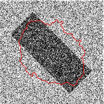
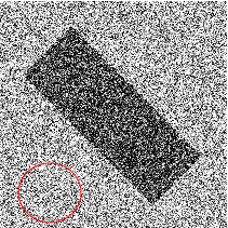
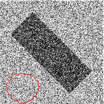
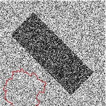
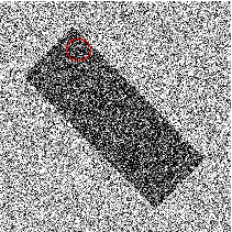
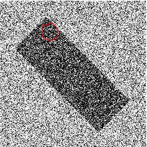
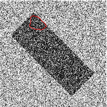
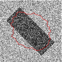
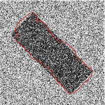
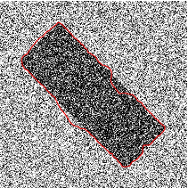
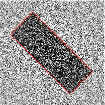
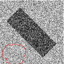
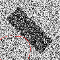
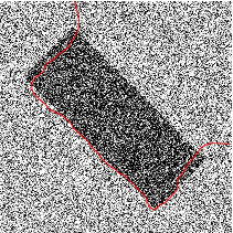
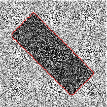
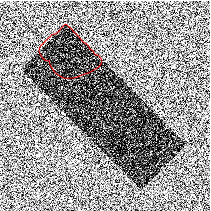
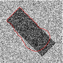
The benefits of acceleration can already been seen, even for this simplest starting kinetic energy model (and for the simplest case of $k$=2 where the gradient force term remains time-independent) by comparing Figures 4 and 4. In Figure 4 we see three different initial contour placements (top, middle, bottom) evolving from left-to-right, each getting stuck in a different local minimizers due to noise, all of which lie very far away from the desired much deeper minimizer along the rectangle boundary. Of course, as always, stronger regularizing terms could be added to the active contour energy functional (or the potential energy in the accelerated scheme) in order to impose smoothness on the contour, thereby making it resistant to noise. However, the point of this synthetic experiment was to create an energy landscape littered with literally tens of thousands (perhaps even hundreds of thousands) of local minimizers in order to demonstrate the effects of acceleration. Furthermore, stronger regularization would come with the additional sacrifice of being unable to capture the sharp corners of the rectangle as well as higher computational cost resulting from the smaller step size constraint in the PDE discretization.

We will not have to make this sacrifice if we regularize the evolution rather than the contour (as we saw with the Sobolev active contour in Figure 1). Indeed, in Figure 4, we see the effect of applying this simplest accelerated evolution scheme (12) with the same initial contour placements and the same energy functional (without additional regularizing terms). In all three cases, the accelerated PDE system initially pushes the contour past the noise, driving it toward the deeper minimum along the rectangle edge. Just as for the Sobolev active contour case in Figure 1,we see that the accelerated active contour only captures noisy structure near the desired converged result.

3.2.3 Conserved flowable mass model

The kinetic energy in the accelerated formulation is invented to endow the minimization evolution process with helpful dynamics for the sake of faster and more robust convergence. Thus, just as the potential energy does not actually represent a real physical energy, there is no need to impose real physical considerations on the kinetic energy either. Nonetheless, the simple constant density model feels quite unnatural in that it does not preserve total mass if the contour length changes during its evolution: mass is created when the contour expands and is destroyed when the contour contracts.

A more flexible and natural way to attribute mass to the evolving contour is to consider an arbitrary and independent distribution of mass along the contour which evolves as the curve evolves. As such, the mass density $\rho$ can vary both spatially and temporarily, while the total integrated mass is still conserved. In such a model, though, not only does mass evolve as a result of contour shape deformation, but it may also flow along the contour without changing its geometry (therefore contributing to the kinetic energy without affecting the potential energy). A simple interpretation would be that the contour shape represents a moving container for a fluid which not only gets pushed around by the extrinsic motion of the container but which may also flow with an independent relative internal speed $v$ inside of the container (i.e. along the tangent direction of the contour). As such, the velocity of each mass particle at a given contour point would be the sum of the contour velocity and the internal mass flow velocity.

$$v=\mbox{internal mass flow speed},\qquad\mbox{total mass velocity}=\frac{\partial C}{\partial t}+v\frac{\partial C}{\partial s}$$

This suggests a more general kinetic energy model as follows

$${\bf T}=\int_{C}\frac{1}{2}\rho\left\|\frac{\partial C}{\partial t}+v\frac{\partial C}{\partial s}\right\|^{2}ds$$ (15)

but with the density evolution constrained by the following continuity equation to ensure local conservation of mass.

$$\underbrace{\frac{\partial\rho}{\partial t}+\frac{\partial}{\partial s}(\rho v)}_{\mbox{mass change}}+\rho\,\underbrace{\left(\frac{\partial^{2}C}{\partial s\partial t}\cdot\frac{\partial C}{\partial s}\right)}_{\mbox{length change}}=0$$ (16)

The latter may be incorporated as a Lagrange multiplier constraint when computing the Euler-Lagrange equation of the generalized action integral (6). This results in the following second order PDE’s which, together with (16), yield the accelerated system as a coupled evolution of $C$ along with the auxiliary mass density $\rho$ and internal flow $v$ field responsible for these helpful dynamics.

$$\frac{\partial^{2}C}{\partial t^{2}}\cdot N =-\left(2v\,\frac{\partial^{2}C}{\partial s\partial t}+v^{2}\frac{\partial^{2}C}{\partial s^{2}}+\frac{k+1}{t}\frac{\partial C}{\partial t}\right)\cdot N+\frac{\lambda k^{2}t^{k-2}f}{\rho}$$ (17)

$$\frac{\partial v}{\partial t} =-\left(\frac{\partial^{2}C}{\partial t^{2}}+v\,\frac{\partial^{2}C}{\partial s\partial t}+\frac{k+1}{t}\frac{\partial C}{\partial t}\right)\cdot\frac{\partial C}{\partial s}-\left(\frac{\partial v}{\partial s}+\frac{k+1}{t}\right)v$$

Notice in this flowable conserved mass model, that only the normal component of the curve acceleration $\frac{\partial^{2}C}{\partial t^{2}}$ is governed by the Euler-Lagrange equation. The tangential acceleration, even though it affects the internal mass flow, can be chosen freely. We may exploit this degree of freedom to keep the tangential velocity of the curve equal to zero, thus keeping the evolution purely geometric. Accordingly, and just as in the constant density case, we may convert the second order system (17) into a first order geometric system of PDE’s. In particular, if we start out with zero initial velocity, we obtain the following equivalent system of three coupled evolution PDE’s for $C$, $V$, and $\rho$ which, in contrast with the constant density scheme, also avoids the calculation of curvature.

$$\overbrace{\frac{\partial V}{\partial t}}^{\mbox{acceleration}}\!\!\!\!\!\!\!\! =\frac{\lambda k^{2}t^{k-2}}{\rho}\overbrace{f\,N}^{-\mbox{gradient}}-\overbrace{\left(V\cdot\frac{\partial C}{\partial s}\right)\frac{\partial V}{\partial s}}^{\mbox{advection}}-\overbrace{\frac{k+1}{t}V}^{\mbox{friction}}$$ (18)

$$\frac{\partial C}{\partial t}= \underbrace{(V\cdot N)}_{\beta}N,\qquad\underbrace{\frac{\partial\rho}{\partial t}=-\left(V\cdot\frac{\partial C}{\partial s}\right)\frac{\partial\rho}{\partial s}-\rho\,\frac{\partial V}{\partial s}\cdot\frac{\partial C}{\partial s}}_{\mbox{mass preservation}}$$

Here the velocity field defined as $V=vT+\beta N$ captures both the tangential flow of the mass as well as the normal flow of the curve itself. As in the constant density model, we see that the evolution of the contour remains purely geometric (only in the normal direction), and thus with suitable spatial extension functions $\hat{V}(x,t)$ and $\hat{\rho}(x,t)$ this system can easily be adapted to the level set framework as well. One notable difference, however, is that evolution equation for the level set function $\psi$ itself, becomes linear in this case.

$$\frac{\partial\psi}{\partial t}=\hat{V}\cdot\nabla\psi$$ (19)

3.3 Mixing optimization dynamics with physical time dynamics

Again, while the kinetic energy models, including their attributed mass density functions $\rho$, are invented purely for the sake of improved optimization, there may be applications in which physically meaningful considerations could nonetheless be usefully blended into the optimization dynamics. Two particular application areas where very strong connections could be made include dynamic tracking as well as optimal mass transport.

3.3.1 Connections with dynamic tracking

Niethammer et. al. [36, 37, 38] introduced a new geometric dynamical active contour model that has strong connections to the present work. The motivation is visual tracking. The authors make the point that the use of active contours is typically preformed statically. More specifically, the active contour captures the given object at a certain time $t$ and then some prediction procedure is employed to give a reasonable initial placement at time $t+1$. The problem is that the curve evolution gets decoupled from the dynamics of the target. The standard dynamic approaches are marker particle based and thus lose the advantages of the level set methodology. the shortcomings of such particle-based implementations. The works of [36, 37, 38] develop a straightforward, efficient, level set based approach for dynamic curve evolution which removes the separation of segmentation and prediction, while preserving the many advantages of level set formulations. The key idea is based on the minimization of novel energy functional that adds dynamics into the geodesic active contour framework.

More precisely, the above approach develops dynamical geodesic snake models for visual tracking based on the classical action ${\bf T}-{\bf U}$ using constant density mass models. This endowed the moving contour with dynamics in actual physical time which could be used in the context of dynamic observers [39].

Such a scheme for frame-to-fame evolution of a contour within a video would pair very naturally, for example, with the simplest-case optimization dynamics from Section 3.2.2 using the same kinetic energy model (11), but in the context of the generalized action (5) for static optimization within each individual video frame. Conversely, the more general kinetic energy models outlined in Section 3.2.3 for optimization using the generalized action, could be similarly be adapted to the the problem of visual tracking using the classical action.

3.3.2 Connections with optimal mass transport

The conserved evolutionary mass model underlying the accelerated system (18) begins to exhibit clear connections to problems in optimal mass transport [23, 3, 1, 53], especially in the fluid-dynamical formulation of Benamou and Brenier [3].

Optimal mass transport is a very old problem first introduced by the civil engineer Monge in 1781 [28] and concerned finding the optimal way, in the sense of minimal transportation cost, of moving a pile of soil from one site to another. This problem of optimal mass transport (OMT) was given a modern formulation in the work of Kantorovich [22, 23], and so is now known as the Monge–Kantorovich (MK) problem. As originally formulated, the problem has no explicit dynamics, and basically leads to a metric on probability densities, the Wasserstein distance. Optimal mass transport is a very active area of research with applications to numerous disciplines including probability, econometrics, fluid dynamics, automatic control, transportation, statistical physics, shape optimization, expert systems, and meteorology.

A major development in optimal mass transport theory was realized in the seminal dynamic approach to optimal mass transport by Benamou and Brenier [3]. These authors base their approach to OMT on ideas from fluid mechanics via the minimization of a kinetic energy functional subject to a continuity constraint.

The work described above is very much in line with the latter dynamics approach. In fact, given that the mass is introduced as an independent auxiliary variable for the sake of acceleration, we may just as easily allow it to live within the contour interior rather than along the contour boundary. The resulting region based extension of the kinetic energy model (15) would then match the functional whose minimizer, as demonstrated Benamou and Brenier, yields a flow of diffeormorphisms which minimize the Wasserstein distance between the mass distributions at any two instances along its trajectory (including the initial and final distributions).

3.4 Accelerated Active Surfaces

The accelerated active contour models developed in Section 3.2 offer a more robust evolution framework for generic contour based optimization problems, just as the class of Sobolev active contour models introduced earlier. Both methodologies regularize the optimization process, without imposing regularity on the final optimized result, greatly boosting the evolving contour’s resistance to spurious or shallow local minimizers. In both cases, this desirable property is achieved by effectively averaging contributions from several local gradient forces in order to determine the instantaneous evolution of any given point on the curve.

In the case of Sobolev active contours, this averaging is done spatially at each fixed time instant by an effective convolution along the curve. Unfortunately, while special tricks exist to do this quickly for closed curves, they do not apply to surfaces or higher dimensional manifolds, where Laplace-Beltrami style PDE’s must instead be solved along the surface at every time instant in order to calculate the Sobolev gradeint.

Accelerated active contour models, on the other hand, perform a temporal rather than spatial averaging. As a particle along the curve accelerates, its instantaneous velocity represents the accumulation of local gradient information over its recently traveled trajectory, rather than the accumulation of local gradient information from its neighboring contour points at the same instant in time. An important advantage of the time-based averaging, in contrast with the instantaneous spatially-based averaging in Sobolev style active contours, is that the same computational speed up in 2D will apply equally in 3D and higher.

In the case of geometric active surfaces, we start with a potential energy which depends only upon the geometric shape of the contour $S$ (again, as in the contour case, not its parameterization). Under these assumptions the first variation of the potential energy will have the following form

$$\delta{\bf U} =-\int_{S}f\,(\delta C\cdot N)\,dA$$

where $fN$ represents a force along the unit normal $N$ at each point on the surface $S$ and where $dA$ denotes the surface area measure. The implicit level set framework is particularly convenient for active surfaces given the complexities of dealing with 3D meshes. In the level set framework, the (non-accelerated) gradient descent surface evolution PDE has the same form as in 2D, but is applied to a 3D grid instead. Namely

$$\frac{\partial\psi}{\partial t}=-\hat{f}\|\nabla\psi\|$$

where $\hat{f}(x,t)$ denotes a spatial extension of $f$ to points away from the surface. Narrow band methods are especially important in 3D to keep the computational cost of updating the level set function $\psi$ to a minimum (as well as limiting the neighborhood where extension functions such as $\hat{f}$ need to be computed and evolved).

In the simplest constant density model case, applied to surfaces. the kinetic energy term for the accelerated model will have a similar form but with the density $\rho$ interpreted per unit surface area.

$${\bf T}=\frac{1}{2}\rho\int_{S}\left(\frac{\partial S}{\partial t}\cdot\frac{\partial S}{\partial t}\right)dA$$

Computing the Euler-Lagrange equation of the generalized action integral (6) and writing it in the level set framework yields the same system of first order PDE’s as in the contour case, except now in 3D dimensions,

$$\frac{\partial\psi}{\partial t}=-\hat{\beta}\|\nabla\psi\|,\qquad\frac{\partial\hat{\beta}}{\partial t}=\frac{\lambda k^{2}t^{(k-2)}}{\rho}\hat{f}+\nabla\cdot\left(\frac{1}{2}\hat{\beta}^{2}\frac{\nabla\psi}{\|\nabla\psi\|}\right)-\frac{k+1}{t}\hat{\beta}$$

where $\hat{f}(x,t)$ and $\hat{\beta}(x,t)$ denote 3D spatial extensions of $f$ and $\beta$ respectively.

3.5 Acceleration with spatial regularity (capturing Sobolev gradient properties)

There are several ways in the PDE framework that we may seek to combine the spatial averaging of gradient information inherent to Sobolev gradient descent with the temporal averaging of gradient information inherent to acceleration, while still remaining fully within the accelerated framework, bypassing the linear operator inversion required in the Sobolev framework. We present two different strategies for obtaining the best-of-both.

3.5.1 Adding velocity diffusion

A simple way to incorporate spatial averaging in the acceleration process would be to heuristically add a diffusion term in the velocity update. For a concrete example, in the conserved flowable-mass acceleration strategy for active contours outlined in Section 3.2.3, we could augment the acceleration PDE (18) as follows (the coupled density evolution PDE would remain the same)

$$\overbrace{\frac{\partial V}{\partial t}}^{\mbox{acceleration}} =\frac{\lambda k^{2}t^{k-2}}{\rho}\overbrace{f\,N}^{\mbox{gradient}}-\overbrace{\left(V\cdot\frac{\partial C}{\partial s}\right)\frac{\partial V}{\partial s}}^{\mbox{advection}}-\overbrace{\frac{k+1}{t}V}^{\mbox{friction}}+\overbrace{\tau\frac{\partial^{2}V}{\partial s^{2}}}^{\mbox{diffusion}}$$

where $\tau>0$ represents a tunable diffusion coefficient. Large values of $\tau$ would give preferential treatment to coarse scale deformations of the evolving contour during the early stages of evolution, with finer scale deformations gradually folding in more and more as the contour converges toward a steady state configuration.

Such a coarse-to-fine behavior would be consistent with that of a Sobolev active contour. In fact, diffusion over a finite amount of time is similar to convolution with a smoothing kernel, which is indeed one way to relate the velocity field of a Sobolev active contour with the simple gradient field $fN$. As such, the incorporation of a diffusion term into the acceleration PDE is the closest and most direct way to endow the accelerated active contour with additional coarse-to-fine Sobolev active contour behaviors without directly employing Sobolev norms in the definition of the kinetic energy (which would would require full linear operator inversion at every time step during the accelerated flow, just as in actual Sobolev gradient flows).

A key difference of such an added diffusion term, compared to Sobolev active contours, is that this smoothing process of the gradient field along the contour is carried out concurrently with the accelerated contour evolution itself, rather than statically at each separate time step. As such, if the diffusion coefficient $\tau$ is small enough to allow stable discretization of the PDE with the same time step dictated by the other first order terms, then no additional computational cost is incurred. As the diffusion coefficient is increased, however, the discrete CFL conditions arising from the added second-order diffusion term will begin to dominate in the numerical implementation of the PDE and require smaller and smaller time steps. This could significantly increase the computational cost as more and more numerical iterations will be needed to simulate the same amount of accelerated flow time.

Given that a sufficiently small amount of diffusion costs essentially nothing in the PDE discretization, however, it doesn’t make sense to ignore this benefit from an optimization standpoint. Methodical schemes guided purely by numerical considerations can be devised to add velocity diffusion coefficients that will maximally boost the regularity of the accelerated evolution with minimal or no added computational cost. Such free gains from small amounts of diffusion may be stretched the farthest by allowing variable diffusion coefficients which can be chosen based on evolving CFL conditions relevant to the PDE discreteizations prior to considering the added diffusion terms.

3.5.2 Incorporating mass potential energy

An independent approach that would add spatial regularization to the acceleration process, again without imposing any added regularity to the converged result, would be to attach not only a kinetic energy term to the artificially attributed mass, but also an extra potential energy term ${\bf U}_{mass}$ which favors a smoother evolution of the mass itself (and therefore of the object to which the auxiliary density function is attributed). This opens up a whole new design feature for accelerated PDE’s which would allow us to incorporate coarse-to-fine evolution properties which are qualitatively similar to those of Sobolev gradient flows, but without the heavy computational cost.

We foresee at least two criteria that should be satisfied when designing the mass potential energy term ${\bf U}_{mass}$

1. The minimum achievable mass potential energy should be independent of the configuration of the original variable being optimized (for example, in the active contour case, it should achievable for any possible contour shape) so that the final converged result, which will correspond to a locally minimal total potential energy, will not be influenced by the added mass potential energy term but only by the original potential energy term to be minimized. As such, the incorporation of ${\bf U}_{mass}$ will affect only the accelerated evolution dynamics, without changing the original energy landscape.

2. The first variation $\delta{\bf U}_{mass}$ should not contain second or higher order derivatives of the density function $\rho$ (nor of its flow velocity $V$) which would, like the diffusion strategy described earlier, impose stronger discrete time step restrictions on the numerical discretization of the accelerated PDE system.

In order to work out a concrete example, we revisit the accelerated active contour model using the conserved flowable mass strategy outlined in Section 3.2.3, in which we suggested that the evolving contour may be thought of as a moving container of fluid (the attributed mass variable), and that the fluid is pushed around by the moving container while also flowing within the container. If the fluid is compressible, then its density can vary during this evolution, otherwise it must remain constant, which undermines the flexibility of this scheme compared to the simpler constant density scheme already developed beforehand in Section 3.2.2. Yet we can still give physical intuition to the more flexible flowable mass model, even if we consider the mass as an incompressible fluid. We simply imagine that the fluid has a variable height at each point within its container (in this case, along the contour). This allows us to naturally define a potential energy for the mass configuration, by relating the density function $\rho$ to the fluid height.

Using this fluid height model, we may construct the mass potential energy connected with an arclength increment $ds$ along the curve by first noting that the associated mass differential is given by $dm=\rho\,ds$ and then equating the mass density $\rho$ along the contour to a constant fluid density $\sigma$ scaled by the local fluid height $h$. Given that the average height of the fluid column over $ds$ would be $h/2$, we may write its potential energy as $\frac{h}{2}\,g\,dm$ where $g$ represents a gravitational constant. Combining these relationships yields

$$d{\bf U}=\frac{g}{2\sigma}\,\rho^{2}ds$$

which, if we choose $\sigma=1$ (without any loss of generality since $g$ can be chosen arbitrarily), gives the following expression for the mass potential energy.

$$g\int_{C}\frac{1}{2}\rho^{2}ds$$

However, while this satisfies our second criterion (its first variation will not involve second order derivatives of $\rho$ or of the flow velocity $V$), it fails our first criterion. To see this, note that lowest potential energy mass distribution for a given curve (subject to the conservation constraint) is achieved by the constant height distribution $\rho=\frac{M}{L}$, where $M$ denotes the constant total conserved mass and where $L=\int_{C}ds$ denotes the total arclength of the contour.

$$\min_{\rho}\left(g\int_{C}\frac{1}{2}\rho^{2}ds\right)=\frac{g}{2}\frac{M^{2}}{L}$$

From this expression, we can see that scaling this potential energy by the length of the curve will make the minimum achievable potential energy $\frac{g}{2}M^{2}$ become independent of the curve $C$. This leads to the following candidate for a mass potential energy which also satisfies our first criterion.

$${\bf U}_{mass}=g\,L\int_{C}\frac{1}{2}\rho^{2}ds$$ (20)

Adding this to the purely contour based potential energy (Section 3.2.1), which does not depend on the artificially added mass, and recomputing the Euler-Lagrange equations for the generalized action integral (6) will yield a new system of accelerated PDE’s in which the gradient forces influencing the acceleration will depend both on the mass distribution as well as the functional to be minimized. Since the minimum constant density mass potential can be achieved for any contour configuration, we know that at steady state, we will have a constant mass density. If we initialize with a constant mass density as well, then the acceleration dynamics will favor (but not constrain) moving the mass along evolution paths that keep the density spatially constant. Translations or uniform rescaling of the curve would therefore become preferential evolutions, just as for Sobolev active contours, especially with larger choices of the tunable gravitational constant $g$.

3.6 Incorporating stochastic acceleration terms

Finally, the accelerated PDE framework, unlike the gradient descent PDE framework, offers a numerical opportunity to introduce random noise into the evolution process without destroying the continuity of the evolution process nor of the evolving object. For example, in the active contour acceleration scheme (18), we could replace the added diffusion term suggested in Section 3.5, with a stochastic term as follows

$$\overbrace{\frac{\partial V}{\partial t}}^{\mbox{acceleration}}\!\!\!\!\!\!\!\!=\frac{\lambda k^{2}t^{k-2}}{\rho}\overbrace{f\,N}^{\mbox{gradient}}-\overbrace{\left(V\cdot\frac{\partial C}{\partial s}\right)\frac{\partial V}{\partial s}}^{\mbox{advection}}-\overbrace{\frac{k+1}{t}V}^{\mbox{friction}}+\overbrace{\tau{\cal W}}^{\mbox{noise}},\qquad\frac{\partial C}{\partial t}=(V\cdot N)N$$

where ${\cal W}$ represents samples drawn from a random noise process and $\tau$ is a positive tunable coefficient (similar to the diffusion coefficient in Section 3.5). Since the noise is added to the acceleration, it gets twice integrated in the construction of the updated contour (or surface) and therefore does not immediately interfere with the continuity nor the first order differentiability of the evolving variable. As such, both the velocity $V$ itself as well as the unit normal $N$ of the contour, remain continuous for the the coupled contour evolution equation. The contour therefore maintains regularity (at least short term). Furthermore, since upwind differencing methods are utilized in the numerical calculation of $\frac{\partial V}{\partial s}$ in the acceleration advection term, discontinuities in the first derivative of $V$ do not pose a problem as only one-sided derivatives are required. In the case of shocks, a viscosity solution will be approximated by a proper discretization.

Adding random noise to a standard (non-accelerated) gradient descent contour PDE, on the other hand,

$$\overbrace{\frac{\partial C}{\partial t}}^{\mbox{velocity}}=\overbrace{f\,N}^{\mbox{gradient}}+\overbrace{\tau{\cal W}}^{\mbox{noise}}$$

has never been a viable option since noise added directly to the velocity is integrated only once, which does not maintain continuity in the unit normal $N$ of the evolving contour. As such, the contour would immediately become irregular. As such, accelerated PDE’s open up a whole new avenue for the inclusion of stochastic terms (as often exploited in finite dimensional optimization problems) which offer an additional strategy for increased resistance to spurious or shallow local minimizers. The potential benefit of such a random noise term would be to provide a second and independent mechanism (beyond the acceleration itself) to perturb the optimization flow away from saddle points or shallow minimizers. Once kinetic energy has been accumulated, the added benefit of such a term is likely to be negligible. However, unlucky initializations (assuming zero initial velocity) near local minimizers or saddle points, could benefit from a noise driven term in the early stages while momentum is just begining to accumulate. Note that such a strategy is not the same as stochastic gradient descent, and should not be confused with the recently developed PDE methods in [12, 13] which specifically improve upon stochastic gradinent descent technqiues used in training deep neural networks.

4 Appendix: Derivations of various numbered equations

calculation of equation (8) Differentiating (7) with respect to the arclength parameter $s$ yields $\displaystyle\frac{\partial^{2}C}{\partial s\partial t}$ $\displaystyle=\frac{\partial\alpha}{\partial s}T+\alpha\underbrace{\frac{\partial T}{\partial s}}_{\kappa N}+\frac{\partial\beta}{\partial s}N+\beta\underbrace{\frac{\partial N}{\partial s}}_{-\kappa T}=\left(\frac{\partial\alpha}{\partial s}-\beta\kappa\right)T+\left(\frac{\partial\beta}{\partial s}+\alpha\kappa\right)N$ and differentiating $T=\frac{\partial C}{\partial s}$ yields $\displaystyle\frac{\partial T}{\partial t}$ $\displaystyle=\frac{\partial}{\partial t}\frac{\partial C}{\partial s}=\frac{\partial}{\partial t}\left(\frac{\frac{\partial C}{\partial p}}{\left\|\frac{\partial C}{\partial p}\right\|}\right)=\frac{\frac{\partial^{2}C}{\partial t\partial p}}{\left\|\frac{\partial C}{\partial p}\right\|}-\frac{\frac{\partial C}{\partial p}}{\left\|\frac{\partial C}{\partial p}\right\|^{2}}\frac{\partial}{\partial t}\left\|\frac{\partial C}{\partial p}\right\|=\frac{\frac{\partial^{2}C}{\partial p\partial t}}{\left\|\frac{\partial C}{\partial p}\right\|}-\frac{\frac{\partial C}{\partial p}}{\left\|\frac{\partial C}{\partial p}\right\|^{2}}\frac{\frac{\partial^{2}C}{\partial p\partial t}\cdot\frac{\partial C}{\partial p}}{\left\|\frac{\partial C}{\partial p}\right\|}$ $\displaystyle=\frac{\partial^{2}C}{\partial s\partial t}-T\left(\frac{\partial^{2}C}{\partial s\partial t}\cdot T\right)=\left(\frac{\partial^{2}C}{\partial s\partial t}\cdot N\right)N=\left(\frac{\partial\beta}{\partial s}+\alpha\kappa\right)N$ which gives the first part of (8) with the second part due the rotation relationship between $T$ and $N$.

calculation of equation (12) Letting $C(p,t)$ denote a parameterization of the evolving curve $C$ with a time-independent spatial parameter $p$ and with $s$ denoting the time-dependent arclength parameter we compute (ignoring temporary boundary terms when applying integration by parts and assuming a closed curve so that spatial boundary terms cancel): $\displaystyle\delta\int_{0}^{1}\frac{t^{k+1}}{k}\left({\bf T}-\lambda k^{2}t^{k-2}{\bf U}\right)\,dt=\delta\int_{0}^{1}\left(\int_{0}^{1}\frac{1}{2}\frac{t^{k+1}}{k}\rho\frac{\partial C}{\partial t}\cdot\frac{\partial C}{\partial t}\,ds-\lambda kt^{2k-1}{\bf U}\right)\,dt=\int_{0}^{1}\delta\left(\int_{0}^{1}\frac{1}{2}\frac{t^{k+1}}{k}\rho\frac{\partial C}{\partial t}\cdot\frac{\partial C}{\partial t}\left\|\frac{\partial C}{\partial p}\right\|dp-\lambda kt^{2k-1}{\bf U}\right)\,dt$ $\displaystyle=\int_{0}^{1}\frac{\rho}{k}\left(\int_{0}^{1}\frac{1}{2}t^{k+1}\left(\frac{\partial C}{\partial t}\cdot\delta\frac{\partial C}{\partial t}\left\|\frac{\partial C}{\partial p}\right\|+\frac{1}{2}\left\|\frac{\partial C}{\partial t}\right\|^{2}\delta\left\|\frac{\partial C}{\partial p}\right\|\right)dp-\frac{\lambda k^{2}t^{2k-1}}{\rho}\delta{\bf U}\right)\,dt$ $\displaystyle=\int_{0}^{1}\frac{\rho}{k}\left(\int_{0}^{1}-\frac{\partial}{\partial t}\left(t^{k+1}\frac{\partial C}{\partial t}\left\|\frac{\partial C}{\partial p}\right\|\right)\cdot\delta C+\frac{1}{2}t^{k+1}\left\|\frac{\partial C}{\partial t}\right\|^{2}\delta\frac{\partial C}{\partial p}\cdot\frac{\partial C}{\partial s}\,dp+\frac{\lambda k^{2}t^{2k-1}}{\rho}\int_{C}f\,(\delta C\cdot N)\,ds\right)\,dt$ $\displaystyle=\int_{0}^{1}\frac{\rho}{k}\left(\int_{0}^{1}-t^{k+1}\frac{\partial^{2}C}{\partial t^{2}}\left\|\frac{\partial C}{\partial p}\right\|-(k+1)t^{k}\frac{\partial C}{\partial t}\left\|\frac{\partial C}{\partial p}\right\|-t^{k+1}\frac{\partial C}{\partial t}\frac{\partial}{\partial t}\left\|\frac{\partial C}{\partial p}\right\|-\frac{1}{2}t^{k+1}\frac{\partial}{\partial p}\left(\left\|\frac{\partial C}{\partial t}\right\|^{2}\frac{\partial C}{\partial s}\right)\cdot\delta C\,dp+\frac{\lambda k^{2}t^{2k-1}}{\rho}\int_{C}fN\cdot\delta C\,ds\right)\,dt$ $\displaystyle=\int_{0}^{1}\frac{t^{k+1}}{k}\rho\left(\int_{0}^{1}\left(-\frac{\partial^{2}C}{\partial t^{2}}\left\|\frac{\partial C}{\partial p}\right\|-\frac{k+1}{t}\frac{\partial C}{\partial t}\left\|\frac{\partial C}{\partial p}\right\|-\frac{\partial C}{\partial t}\left(\frac{\partial^{2}C}{\partial p\partial t}\cdot\frac{\partial C}{\partial s}\right)-\frac{1}{2}\frac{\partial}{\partial p}\left(\left\|\frac{\partial C}{\partial t}\right\|^{2}\frac{\partial C}{\partial s}\right)\right)\cdot\delta C\,dp+\frac{\lambda k^{2}t^{k-2}}{\rho}\int_{C}fN\cdot\delta C\,ds\right)\,dt$ $\displaystyle=\int_{0}^{1}\frac{t^{k+1}}{k}\rho\int_{C}\underbrace{\left(-\frac{\partial^{2}C}{\partial t^{2}}-\frac{k+1}{t}\frac{\partial C}{\partial t}-\left(\frac{\partial^{2}C}{\partial s\partial t}\cdot\frac{\partial C}{\partial s}\right)\frac{\partial C}{\partial t}-\frac{\partial}{\partial s}\left(\frac{1}{2}\left\|\frac{\partial C}{\partial t}\right\|^{2}\frac{\partial C}{\partial s}\right)+\frac{\lambda k^{2}t^{k-2}}{\rho}fN\right)}_{\mbox{Set to zero for Euler-Lagrange equation}}\cdot\delta C\,ds\,dt$

calculation of equation (13) Decomposing the acceleration $C_{tt}$ into tangential and normal components yields $\displaystyle\frac{\partial^{2}C}{\partial t^{2}}$ $\displaystyle=-\frac{k+1}{t}\frac{\partial C}{\partial t}-\left(\frac{\partial^{2}C}{\partial s\partial t}\cdot\frac{\partial C}{\partial s}\right)\frac{\partial C}{\partial t}-\left(\frac{\partial^{2}C}{\partial s\partial t}\cdot\frac{\partial C}{\partial t}\right)\frac{\partial C}{\partial s}-\frac{1}{2}\left\|\frac{\partial C}{\partial t}\right\|^{2}\frac{\partial^{2}C}{\partial s^{2}}+\frac{\lambda k^{2}t^{k-2}f}{\rho}N$ $\displaystyle=-\frac{k+1}{t}\frac{\partial C}{\partial t}-\left(\frac{\partial\alpha}{\partial s}-\beta\kappa\right)\frac{\partial C}{\partial t}-\left(\alpha\frac{\partial\alpha}{\partial s}+\beta\frac{\partial\beta}{\partial s}\right)T-\frac{\alpha^{2}+\beta^{2}}{2}\kappa N+\frac{\lambda k^{2}t^{k-2}f}{\rho}N$ $\displaystyle\frac{\partial^{2}C}{\partial t^{2}}\cdot T$ $\displaystyle=-\left(\frac{k+1}{t}+\frac{\partial\alpha}{\partial s}-\beta\kappa\right)\alpha-\left(\alpha\frac{\partial\alpha}{\partial s}+\beta\frac{\partial\beta}{\partial s}\right)=-\left(\frac{k+1}{t}+2\frac{\partial\alpha}{\partial s}-\beta\kappa\right)\alpha-\beta\frac{\partial\beta}{\partial s}$ $\displaystyle\frac{\partial^{2}C}{\partial t^{2}}\cdot N$ $\displaystyle=-\left(\frac{k+1}{t}+\frac{\partial\alpha}{\partial s}-\beta\kappa\right)\beta-\frac{\alpha^{2}+\beta^{2}}{2}\kappa+\frac{\lambda k^{2}t^{k-2}f}{\rho}$ Now inserting these acceleration components into (10) yields $\displaystyle\frac{\partial\alpha}{\partial t}$ $\displaystyle=\underbrace{-\left(\frac{k+1}{t}+2\frac{\partial\alpha}{\partial s}-\beta\kappa\right)\alpha-\beta\frac{\partial\beta}{\partial s}}_{\frac{\partial^{2}C}{\partial t^{2}}\cdot T}+\beta\left(\frac{\partial\beta}{\partial s}+\alpha\kappa\right)=\left(-\frac{k+1}{t}-2\frac{\partial\alpha}{\partial s}+2\beta\kappa\right)\alpha$ $\displaystyle\frac{\partial\beta}{\partial t}$ $\displaystyle=\underbrace{-\left(\frac{k+1}{t}+\frac{\partial\alpha}{\partial s}-\beta\kappa\right)\beta-\frac{\alpha^{2}+\beta^{2}}{2}\kappa+\frac{\lambda k^{2}t^{k-2}f}{\rho}}_{\frac{\partial^{2}C}{\partial t^{2}}\cdot N}-\alpha\left(\frac{\partial\beta}{\partial s}+\alpha\kappa\right)=-\frac{k+1}{t}\beta-\frac{\partial}{\partial s}(\alpha\beta)+\left(\frac{1}{2}\beta^{2}-\frac{3}{2}\alpha^{2}\right)\kappa+\frac{\lambda k^{2}t^{k-2}f}{\rho}$ Given zero initial velocity ($\alpha$=0 and $\beta$=0), simple inspection shows that $\alpha$ remains zero, leading to the simplified evolution (13).

calculation of equation (14) Assuming we represent the evolving curve $C(p,t)$ as the zero level set of an evolving function $\psi(x,t)$ and letting $\hat{\beta}(x,t)$ denote an evolving spatial extension of the evolving normal speed function $\beta(p,t)$ along curve, then we have $$\psi\left(C(p,t),t\right)=0\quad\mbox{and}\quad\hat{\beta}\left(C(p,t),t\right)=\beta(p,t)$$ Differentiating with respect to $t$ yields $$\frac{\partial\psi}{\partial t}+\nabla\psi\cdot\frac{\partial C}{\partial t}=0\quad\mbox{and}\quad\frac{\partial\hat{\beta}}{\partial t}+\nabla\hat{\beta}\cdot\frac{\partial C}{\partial t}=\frac{\partial\beta}{\partial t}$$ Extending the contour evolution $\frac{\partial C}{\partial t}=\beta N$ to other level sets as $\hat{\beta}\hat{N}$, where $\hat{N}=-\frac{\nabla\psi}{\|\nabla\psi\|}$ (noting that this convention for the extension of the inward unit normal requires that the level set function be negative inside the contour and positive outside), yields $$\frac{\partial\psi}{\partial t}=\hat{\beta}\|\nabla\psi\|\quad\mbox{and}\quad\frac{\partial\hat{\beta}}{\partial t}=\frac{\partial\beta}{\partial t}+\nabla\hat{\beta}\cdot\frac{\hat{\beta}\nabla\psi}{\|\nabla\psi\|}$$ which, after substitution of $\frac{\partial\beta}{\partial t}$ using (13) results in the level set version of the system in (14).

calculation of equation (17) Let us introduce, along with the mass density $\rho$ and its internal flow speed $v$ with respect to the arclength parameter $s$, corresponding variables for the mass density $\mu(p,t)$ and internal flow speed $\xi(p,t)$ with respect to a time-independent contour parameter $p$. These pairs of densities and internal flow speeds are related to each other through the parameterization speed $\left\|C_{p}\right\|$ of the contour as follows. $$\mu=\rho\left\|C_{p}\right\|\quad\mbox{and}\quad v=\xi\,\left\|C_{p}\right\|\quad(\mbox{with matching flux expressions }\mu\,\xi=\rho\,v)$$ (21) Differentiating with respect to $t$, yields the following relationships between the density and flow speed evolution as well. $$\mu_{t}-\mu\,C_{ts}\cdot C_{s}=\rho_{t}\left\|C_{p}\right\|\quad\mbox{and}\quad v_{t}-v\,C_{ts}\cdot C_{s}=\xi_{t}\left\|C_{p}\right\|$$ (22) Applying these substitutions to the kinetic energy (15) and continuity constraint (16) yields $${\bf T}=\int_{0}^{1}\frac{1}{2}\mu\left\|C_{t}+\xi\,C_{p}\right\|^{2}dp\quad\mbox{with mass continuity constraint}\quad\mu_{t}+\left(\mu\,\xi\right)_{p}=0$$ We plug this into the generalized action integral (6) with a Lagrange multiplier function $\lambda(p,t)$ and compute the first variation. $\displaystyle\delta$ $\displaystyle\int_{0}^{1}\frac{t^{k+1}}{k}\left({\bf T}-\lambda k^{2}t^{k-2}{\bf U}\right)+\int_{0}^{1}\lambda\left(\mu_{t}+(\mu\xi)_{p}\right)dp\,dt=\int_{0}^{1}\delta\int_{0}^{1}\frac{1}{2}\frac{t^{k+1}}{k}\mu\,\left\|C_{t}+\xi\,C_{p}\right\|^{2}+\lambda\,\left(\mu_{t}+(\mu\xi)_{p}\right)\,dp-\lambda kt^{2k-1}\delta{\bf U}\,dt$ $\displaystyle=$ $\displaystyle\int_{0}^{1}\int_{0}^{1}\frac{1}{2}\frac{t^{k+1}}{k}\left\|C_{t}+\xi\,C_{p}\right\|^{2}\delta\mu+\frac{t^{k+1}}{k}\mu\,(C_{t}+\xi\,C_{p})\cdot\delta\left(C_{t}+\xi\,C_{p}\right)+\underbrace{\left(\mu_{t}+(\mu\xi)_{p}\right)}_{=0}\delta\lambda+\lambda\,\delta\left(\mu_{t}+(\mu\xi)_{p}\right)+\lambda kt^{2k-1}f\,(\delta C\cdot N)\,\|C_{p}\|\,dp\,dt$ $\displaystyle=$ $\displaystyle\int_{0}^{1}\int_{0}^{1}\frac{1}{2}\frac{t^{k+1}}{k}\left\|C_{t}+\xi\,C_{p}\right\|^{2}\delta\mu+\frac{t^{k+1}}{k}\mu\,(C_{t}+\xi\,C_{p})\cdot C_{p}\,\delta\xi-\lambda_{t}\delta\mu-\lambda_{p}\delta\left(\mu\xi\right)-\left(\frac{t^{k+1}}{k}\mu\,(C_{t}+\xi\,C_{p})\right)_{t}\cdot\delta C-\left(\frac{t^{k+1}}{k}\mu\xi\,(C_{t}+\xi\,C_{p})\right)_{p}\cdot\delta C$ $\displaystyle\qquad+\lambda kt^{2k-1}f\,N\cdot\delta C\,\|C_{p}\|\,dp\,dt$ $\displaystyle=$ $\displaystyle\int_{0}^{1}\int_{0}^{1}\left(\frac{1}{2}\frac{t^{k+1}}{k}\left\|C_{t}+\xi\,C_{p}\right\|^{2}-\lambda_{t}-\lambda_{p}\xi\right)\,\delta\mu+\mu\,\left(\frac{t^{k+1}}{k}(C_{t}+\xi\,C_{p})\cdot C_{p}-\lambda_{p}\right)\,\delta\xi$ $\displaystyle\qquad-\frac{t^{k+1}}{k}\mu\left(\underbrace{\left(\mu_{t}+(\mu\xi)_{p}\right)}_{=0}\,\frac{C_{t}+\xi\,C_{p}}{\mu}+\left(C_{t}+\xi\,C_{p}\right)_{t}+\xi\,\left(C_{t}+\xi\,C_{p}\right)_{p}+\frac{k+1}{t}(C_{t}+\xi\,C_{p})-\frac{\lambda k^{2}t^{k-2}f\,N}{\rho}\right)\cdot\delta C\,dp\,dt$ The optimality conditions with respect to variations $\delta\xi$ and $\delta\mu$ respectively yield $$\lambda_{p}=\frac{t^{k+1}}{k}\left(\xi\,\|C_{p}\|^{2}+C_{t}\cdot C_{p}\right)\quad\mbox{and}\quad\lambda_{t}=\frac{1}{2}\frac{t^{k+1}}{k}\left\|C_{t}+\xi\,C_{p}\right\|^{2}-\xi\lambda_{p}$$ which, when combined, give the following evolution for the Lagrange multiplier $\displaystyle\lambda_{t}$ $\displaystyle=\frac{t^{k+1}}{k}\left(\frac{1}{2}\left\|C_{t}+\xi\,C_{p}\right\|^{2}-\left(\|\xi\,C_{p}\|^{2}+C_{t}\cdot\xi C_{p}\right)\right)=\frac{t^{k+1}}{k}\left(\frac{1}{2}\left\|C_{t}+v\,C_{s}\right\|^{2}-\left(\|v\,C_{s}\|^{2}+C_{t}\cdot v\,C_{s}\right)\right)=\frac{1}{2}\frac{t^{k+1}}{k}\left(\|C_{t}\|^{2}-v^{2}\right)$ We eliminate the Lagrange multiplier by equating $\lambda_{tp}$ and $\lambda_{pt}$ to obtain the following internal flow speed evolution $\displaystyle 0=$ $\displaystyle\lambda_{tp}-\lambda_{pt}=\frac{1}{2}\frac{t^{k+1}}{k}\left(\|C_{t}\|^{2}-v^{2}\right)_{p}-\left(\frac{t^{k+1}}{k}\left(C_{t}+\xi\,C_{p}\right)\cdot C_{p}\right)_{t}$ $\displaystyle 0=$ $\displaystyle\underbrace{\frac{t^{k+1}}{k}}_{\mbox{drop}}\left(\underbrace{C_{t}\cdot C_{tp}}_{\mbox{cancel}}-vv_{p}-C_{tt}\cdot C_{p}-\xi_{t}C_{p}\cdot C_{p}-2\xi\,C_{tp}\cdot C_{p}-\underbrace{C_{t}\cdot C_{tp}}_{\mbox{cancel}}-\frac{k+1}{t}\left(C_{t}+\xi\,C_{p}\right)\cdot C_{p}\right)$ $\displaystyle 0=$ $\displaystyle\underbrace{\|C_{p}\|}_{\mbox{drop}}\left(-vv_{s}-C_{tt}\cdot C_{s}-\underbrace{(\xi_{t}\|C_{p}\|+v\,C_{ts}\cdot C_{s})}_{v_{t}\mbox{ by using \eqref{eq:substitute-evolve}}}-v\,C_{ts}\cdot C_{s}-\frac{k+1}{t}\left(C_{t}+v\,C_{s}\right)\cdot C_{s}\right)$ $\displaystyle v_{t}=$ $\displaystyle-\left(C_{tt}+v\,(C_{t}+v\,C_{s})_{s}+\frac{k+1}{t}\left(C_{t}+v\,C_{s}\right)\right)\cdot C_{s}=-\left(C_{tt}+vC_{ts}+\frac{k+1}{t}C_{t}\right)\cdot C_{s}-\left(v_{s}+\frac{k+1}{t}\right)v$ Finally, the optimality condition with respect to the curve perturbation $\delta C$ yields the following acceleration equation for the contour $\displaystyle 0$ $\displaystyle=C_{tt}+\!\!\!\underbrace{\xi_{t}\|C_{p}\|}_{v_{t}-vC_{ts}\cdot C_{s}}\!\!\!C_{s}+v\,C_{ts}+v\,\left(C_{t}+v\,C_{s}\right)_{s}+\frac{k+1}{t}(C_{t}+v\,C_{s})-\frac{\lambda k^{2}t^{k-2}f}{\rho}N$ $\displaystyle 0$ $\displaystyle=C_{tt}+\left(v_{t}-v\,C_{ts}\cdot C_{s}\right)\,C_{s}+v\,C_{ts}+v\,\left(C_{t}+v\,C_{s}\right)_{s}+\frac{k+1}{t}(C_{t}+v\,C_{s})-\frac{\lambda k^{2}t^{k-2}f}{\rho}N$ $\displaystyle 0$ $\displaystyle=\underbrace{\left(C_{tt}+v\,\left(C_{t}+v\,C_{s}\right)_{s}+\frac{k+1}{t}(C_{t}+v\,C_{s})+v\,C_{ts}\right)}_{\mbox{some vector}}-\underbrace{\left(\left(C_{tt}+v(C_{t}+v\,C_{s})_{s}+\frac{k+1}{t}\left(C_{t}+v\,C_{s}\right)+v\,C_{ts}\right)\cdot C_{s}\right)C_{s}}_{\mbox{its tangential component}}-\frac{\lambda k^{2}t^{k-2}f}{\rho}N$ $\displaystyle 0$ $\displaystyle=\underbrace{\left(C_{tt}+v(C_{t}+v\,C_{s})_{s}+\frac{k+1}{t}\left(C_{t}+v\,C_{s}\right)+vC_{ts}\right)\cdot N}_{\mbox{its normial projection}}-\frac{\lambda k^{2}t^{k-2}f}{\rho}=\left(C_{tt}+2v\,C_{ts}+v^{2}C_{ss}+\frac{k+1}{t}C_{t}\right)\cdot N-\frac{\lambda k^{2}t^{k-2}f}{\rho}$

calculation of equation (18) Plugging the normal and tangential (unconstrained) acceleration components from (17) into (10) yields $\displaystyle\alpha_{t}$ $\displaystyle=\underbrace{C_{tt}\cdot T}_{\mbox{free}}+\beta\left(\beta_{s}+\alpha\kappa\right)$ $\displaystyle\beta_{t}$ $\displaystyle=\underbrace{\left(-2v\,\overbrace{\left(\beta_{s}+\alpha\kappa\right)}^{C_{ts}\cdot N}-v^{2}\overbrace{\kappa}^{C_{ss}\cdot N}-\frac{k+1}{t}\overbrace{\beta}^{C_{t}\cdot N}+\lambda k^{2}t^{k-2}\frac{f}{\rho}\right)}_{C_{tt}\cdot N\mbox{ from equation \eqref{eq:acceleration-flowable}}}-\alpha(\beta_{s}+\alpha\kappa)$ $\displaystyle=-\left(2v+\alpha\right)\beta_{s}-\left(\alpha+v\right)^{2}\kappa-\frac{k+1}{t}\beta+\lambda k^{2}t^{k-2}\frac{f}{\rho}$ $\displaystyle v_{t}$ $\displaystyle=-C_{tt}\cdot T-v\,\overbrace{(\alpha_{s}-\beta\kappa)}^{C_{ts}\cdot T}-\frac{k+1}{t}(\overbrace{\alpha}^{C_{t}\cdot T}+v)-vv_{s}\qquad\left[\mbox{from second part of equation \eqref{eq:acceleration-flowable}}\right]$ $\displaystyle\alpha_{t}+v_{t}$ $\displaystyle=\left(C_{tt}\cdot T+\beta\beta_{s}+\alpha\beta\kappa\right)+\left(-C_{tt}\cdot T-v\,(\alpha_{s}-\beta\kappa)-vv_{s}-\frac{k+1}{t}\left(\alpha+v\right)\right)$ $\displaystyle\left(\alpha+v\right)_{t}$ $\displaystyle=\beta\beta_{s}-\left(\alpha_{s}+v_{s}\right)v+\left(\alpha+v\right)\beta\kappa-\frac{k+1}{t}\left(\alpha+v\right)$ $\displaystyle\rho_{t}+(\rho v)_{s}$ $\displaystyle=-\rho\,\overbrace{\left(\alpha_{s}-\beta\kappa\right)}^{C_{ts}\cdot T}\qquad\qquad\qquad\qquad\qquad\qquad\qquad\qquad\quad\left[\mbox{from equation \eqref{eq:continuity-constraint}}\right]$ We can now rewrite the system as follows. $\displaystyle\alpha_{t}$ $\displaystyle=\underbrace{C_{tt}\cdot T}_{\mbox{free}}+\beta\left(\beta_{s}+\alpha\kappa\right)$ $\displaystyle\beta_{t}$ $\displaystyle=-\beta_{s}v-\left(\alpha+v\right)\beta_{s}-\left(\alpha+v\right)^{2}\kappa-\frac{k+1}{t}\beta+\lambda k^{2}t^{k-2}\frac{f}{\rho}$ $\displaystyle\left(\alpha+v\right)_{t}$ $\displaystyle=-\left(\alpha+v\right)_{s}v+\beta\beta_{s}+\left(\alpha+v\right)\beta\kappa-\frac{k+1}{t}\left(\alpha+v\right)$ $\displaystyle\rho_{t}$ $\displaystyle=-\rho_{s}v-\rho\left(\alpha+v\right)_{s}+\rho\beta\kappa$ where we can see that freedom to choose $C_{tt}\cdot T$ is equivalent to freedom to choose the evolution of $\alpha$. As such, we may conveniently choose $\alpha_{t}=0$. Assuming that we start out with zero initial velocity ($\alpha=\beta=0$) this would mean $\alpha$remains zero, yielding the following simplified system. $\displaystyle\beta_{t}$ $\displaystyle+v\beta_{s}=-v\left(\beta_{s}+v\kappa\right)-\frac{k+1}{t}\beta+\lambda k^{2}t^{k-2}\frac{f}{\rho}$ $\displaystyle v_{t}$ $\displaystyle+vv_{s}=\beta\left(\beta_{s}+v\kappa\right)-\frac{k+1}{t}v$ $\displaystyle\rho_{t}$ $\displaystyle+v\rho_{s}=\rho\left(\beta\kappa-v_{s}\right)$ Finally, we may transform the system by defining $V=vT+\beta N$ to avoid the explicit calculation of curvature. Noting that $$V_{s}=\left(vT+\beta N\right)_{s}=\left(v_{s}-\beta\kappa\right)T+\left(\beta_{s}+v\kappa\right)N$$ and, substituting $\alpha=0$ into (8), to obtain $$T_{t}=\beta_{s}N\quad\mbox{and}\quad N_{t}=-\beta_{s}T$$ we may compute $\displaystyle V_{t}$ $\displaystyle=\left(vT+\beta N\right)_{t}=\left(v_{t}-\beta\beta_{s}\right)T+\left(\beta_{t}+v\beta_{s}\right)N$ $\displaystyle=\left(\underbrace{\beta(\beta_{s}+v\kappa)-vv_{s}-\frac{k+1}{t}v}_{v_{t}}-\beta\beta_{s}\right)T+\left(\underbrace{-v(\beta_{s}+v\kappa)-v\beta_{s}-\frac{k+1}{t}\beta+\lambda k^{2}t^{k-2}\frac{f}{\rho}}_{\beta_{t}}+v\beta_{s}\right)N$ $\displaystyle=-v\underbrace{\left(\left(v_{s}-\beta\kappa\right)T+\left(\beta_{s}+v\kappa\right)N\right)}_{V_{s}}-\frac{k+1}{t}\underbrace{\left(vT+\beta N\right)}_{V}+\left(\lambda k^{2}t^{k-2}\frac{f}{\rho}\right)N$ as well as $$\rho_{t}+\underbrace{v}_{V\cdot T}\rho_{s}=\rho\,\underbrace{(\beta\kappa-v_{s})}_{V_{s}\cdot T}$$

References

- [1] Sigurd Angenent, Steven Haker, and Allen Tannenbaum. Minimizing flows for the monge-kantorovich problem. SIAM J. Math. Analysis, 35:61–97, 2003.
- [2] E. Bardelli, M. Colombo, A. Mennucci, and A. Yezzi. Multiple object tracking via prediction and filtering with a sobolev-type metric on curves. In European Conf. Computer Vision, pages 143–152, 2012.
- [3] J.D. Benamou and Y. Brenier. A computational fluid mechanics solution to the monge-kantorovich mass transfer problem. Numerische Mathematik, 84:375–393, 2000.
- [4] Stephen Boyd and Lieven Vandenberghe. Convex optimization. Cambridge university press, 2004.
- [5] Sébastien Bubeck, Yin Tat Lee, and Mohit Singh. A geometric alternative to nesterov’s accelerated gradient descent. CoRR, abs/1506.08187, 2015.
- [6] Vincent Caselles, Ron Kimmel, and Guillermo Sapiro. Geodesic active contours. International Journal on Comptuer Vision, 22(1):61–79, 1997.
- [7] Antonin Chambolle and Thomas Pock. A first-order primal-dual algorithm for convex problems with applications to imaging. Journal of mathematical imaging and vision, 40(1):120–145, 2011.
- [8] Tony Chan and Luminita Vese. Active contours without edges. IEEE Transactions on Image Processing, 10(2):266–277, 2001.
- [9] Tony F Chan, Selim Esedoglu, and Mila Nikolova. Algorithms for finding global minimizers of image segmentation and denoising models. SIAM journal on applied mathematics, 66(5):1632–1648, 2006.
- [10] G. Charpiat, R. Keriven, J.P. Pons, and O. Faugeras. Designing spatially coherent minimizing flows for variational problems based on active contours. In Int. Conference Computer Vision, 2005.
- [11] Guillaume Charpiat, Olivier Faugeras, and Renaud Keriven. Approximations of shape metrics and application to shape warping and empirical shape statistics. Foundations of Computational Mathematics, 5(1):1–58, 2005.
- [12] Pratik Chaudhari, Adam Oberman, Stanley Osher, Stefano Soatto, and Guillame Carlier. Deep relaxation: partial differential equations for optimizing deep neural networks. arXiv preprint arXiv:1704.04932, 2017.
- [13] Pratik Chaudhari and Stefano Soatto. Stochastic gradient descent performs variational inference, converges to limit cycles for deep networks. arXiv preprint arXiv:1710.11029, 2017.
- [14] Nicolas Flammarion and Francis Bach. From averaging to acceleration, there is only a step-size. In Proceedings of Machine Learning Research, volume 40, pages 658–695, 2015.
- [15] Saeed Ghadimi and Guanghui Lan. Accelerated gradient methods for nonconvex nonlinear and stochastic programming. Math. Program., 156(1-2):59–99, 2016.
- [16] Herbert Goldstein, Charles P. Poole, and John L. Safko. Classical Mechanics. Addison Wesley, 2002.
- [17] Tom Goldstein, Xavier Bresson, and Stanley Osher. Geometric applications of the split bregman method: segmentation and surface reconstruction. Journal of Scientific Computing, 45(1-3):272–293, 2010.
- [18] Berthold K.P. Horn and Brian G. Schunck. Determining optical flow. Artifical Intelligence, 17:185–203, 1981.
- [19] Chonghai Hu, Weike Pan, and James T. Kwok. Accelerated gradient methods for stochastic optimization and online learning. In Y. Bengio, D. Schuurmans, J. D. Lafferty, C. K. I. Williams, and A. Culotta, editors, Advances in Neural Information Processing Systems 22, pages 781–789. Curran Associates, Inc., 2009.
- [20] Shuiwang Ji and Jieping Ye. An accelerated gradient method for trace norm minimization. In Proceedings of the 26th Annual International Conference on Machine Learning, ICML ’09, pages 457–464, 2009.
- [21] Vladimir Jojic, Stephen Gould, and Daphne Koller. Accelerated dual decomposition for map inference. In Proceedings of the 27th International Conference on International Conference on Machine Learning, ICML’10, pages 503–510, 2010.
- [22] Leonid Kantorovich. On the transfer of masses. Dokl. Akad. Nauk. SSSR, 37(7-8):227–220, 1942.
- [23] Leonid Kantorovich. On a problem of monge. Uspekhi Mat. Nauk., 3:225–226, 1948.
- [24] S. Kichenassamy, Arun Kumar, Peter Olver, Allen Tannenbaum, and Anthony Yezzi. Conformal curvature flows: From phase transistions to active vision. Archive for Rational Mechanics and Analysis, 134:275–301, 1996.
- [25] Walid Krichene, Alexandre Bayen, and Peter L Bartlett. Accelerated mirror descent in continuous and discrete time. In C. Cortes, N. D. Lawrence, D. D. Lee, M. Sugiyama, and R. Garnett, editors, Advances in Neural Information Processing Systems 28, pages 2845–2853. Curran Associates, Inc., 2015.
- [26] Huan Li and Zhouchen Lin. Accelerated proximal gradient methods for nonconvex programming. In C. Cortes, N. D. Lawrence, D. D. Lee, M. Sugiyama, and R. Garnett, editors, Advances in Neural Information Processing Systems 28, pages 379–387. Curran Associates, Inc., 2015.
- [27] A. Mennucci, A. Yezzi, and G. Sundaramoorthi. Properties of sobolev-type metrics in the space of curves. Interfaces and Free Boundaries, 10:423–445, 2008.
- [28] G. Monge. Mémoire sur la théorie des déblais et des remblais. In De l’Imprimerie Royale. 1781.
- [29] Indraneel Mukherjee, Kevin Canini, Rafael Frongillo, and Yoram Singer. Parallel boosting with momentum. In H. Blockeel, K. Kersting, S. Nijssen, and F. Zelezny, editors, Machine Learning and Knowledge Discovery in Databases, pages 17–32. Springer, Berlin, 2013.
- [30] Yurii Nesterov. A method of solving a convex programming problem with convergence rate o (1/k2). In Soviet Mathematics Doklady, volume 27, pages 372–376, 1983.
- [31] Yurii Nesterov. Smooth minimization of non-smooth functions. Math. Program., 103(1):127–152, 2005.
- [32] Yurii Nesterov. Accelerating the cubic regularization of newton’s method on convex problems. Math. Program., 112(1):159–181, 2008.
- [33] Yurii Nesterov. Gradient methods for minimizing composite functions. Math. Program., 140(1):125–161, 2013.
- [34] Yurii Nesterov. Introductory Lectures on Convex Optimization: A Basic Course. Springer Publishing Company, Incorporated, 1 edition, 2014.
- [35] Yurii Nesterov and Boris T. Polyak. Cubic regularization of newton method and its global performance. Math. Program., 108(1):177–205, 2006.
- [36] Marc Niethamer and Allen Tannenbaum. Dynamic level sets for visual tracking. In Proceedings of IEEE Conference on Decision and Control, pages 4883–4888, 2003.
- [37] Marc Niethamer and Allen Tannenbaum. Dynamic geodesic snakes for visual tracking. In IEEE Conference on Computer Vision and Pattern Recognition, pages 4883–4888, 2004.
- [38] Marc Niethamer and Allen Tannenbaum. Dynamic geodesic snakes for visual tracking. IEEE Transactions on Automatic Control, 51(4):562–579, 2006.
- [39] Marc Niethamer, Patricio Vela, and Allen Tannenbaum. Geometric observers for dynamically evolving curves. IEEE Trans. Pattern Analysis and Machine Intelligence, 30(6):1093–1108, 2008.
- [40] Brendan O’Donoghue and Emmanuel Candès. Adaptive restart for accelerated gradient schemes. Foundations of Computational Mechanics, 15(3):715–732, 2015.
- [41] Stanely Osher and Nikos Paragios. Geometric Level Set Methods in Imaging, Vision and Graphics. Springer, New York, 2003.
- [42] Stanely Osher and James Sethian. Fronts propagation with curvature dependent speed: Algorithms based on hamilton-jacobi formulations. Journal of Computational Physics, 79:12–49, 1988.
- [43] Thomas Pock, Antonin Chambolle, Daniel Cremers, and Horst Bischof. A convex relaxation approach for computing minimal partitions. In Computer Vision and Pattern Recognition, pages 810–817. IEEE, 2009.
- [44] Guillermo Sapiro. Geometric Partial Differential Equations and Image Analysis. Cambridge Press, Cambridge, England, 2000.
- [45] James Sethian. Level Set Methods: Evolving Interfaces in Geometry, Fluid Mechanics, Computer Vision, and Material Science. Cambridge University Press, 1996.
- [46] Weijie Su, Stephen Boyd, and Emmanuel Candès. A differential equation for modeling nesterov’s accelerated gradient method: Theory and insights. In Advances in Neural Information Processing Systems, pages 2510–2518, 2014.
- [47] G. Sundaramoorthi, J. Jackson, A. Yezzi, and A. Mennucci. Tracking with sobolev active contours. In Proc. Computer Vision and Pattern Recognition, pages 674–680, 2006.
- [48] G. Sundaramoorthi, A. Mennucci, S. Soatto, and A. Yezzi. A new geometric metric in the space of curves, and applications to tracking deforming objects by prediction and filtering. SIAM J. Imaging Sciences, 4:109–145, 2011.
- [49] G. Sundaramoorthi, A. Mennucci, A. Yezzi, and S. Soatto. Tracking deforming objects by filtering and prediction in the space of curves. In Proc. IEEE Conf. Decision and Control, pages 2395–2401, 2009.
- [50] G. Sundaramoorthi, A. Yezzi, and A. Mennucci. Sobolev active contours. In Workshop on Variational Geometric and Level Set Methods in Computer Vision, pages 109–120, 2005.
- [51] Ganesh Sundaramoorthi, Anthony Yezzi, and Andrea Mennucci. Sobolev active contours. Int. J. Computer Vision, 7:345–366, 2007.
- [52] J. L. Troutman. Variational Calclus and Optimal Control. Springer-Verlag, New York, 1996.
- [53] C. Villani. Topics in optimal transportation. In Graduate Studies in Mathematics 58. AMS, Providence RI, 2003.
- [54] Andre Wibisono, Ashia C Wilson, and Michael I Jordan. A variational perspective on accelerated methods in optimization. Proceedings of the National Academy of Sciences, page 201614734, 2016.
- [55] Y. Yang and Ganesh Sundaramoorthi. Shape tracking with occlusions via coarse-to-fine region based sobolev descent. Trans. Pattern Analysis and Machine Intelligence, 2015.