Nonperturbative Analysis of the Electroweak Phase Transition
in the Two Higgs Doublet Model

Abstract

We perform a nonperturbative study of the electroweak phase transition (EWPT) in the two Higgs doublet model (2HDM) by deriving a dimensionally reduced high-temperature effective theory for the model, and matching to known results for the phase diagram of the effective theory. We find regions of the parameter space where the theory exhibits a first-order phase transition. In particular, our findings are consistent with previous perturbative results suggesting that the primary signature of a first-order EWPT in the 2HDM is $m_{A_{0}}>m_{H_{0}}+m_{Z}$.

I Introduction

Accounting for the baryon asymmetry in the present universe is a major unsolved problem in cosmology. One of the leading candidates for a viable mechanism, electroweak baryogenesis (EWBG) Kuzmin:1985mm , suggests that the asymmetry originates from the electroweak phase transition (EWPT) in the early universe. According to the Sakharov conditions Sakharov:1967dj the transition would have to be first order, accompanied by a sizable violation of CP-symmetry. Unfortunately, these conditions immediately rule out EWBG within the minimal Standard Model (SM), as it was demonstrated that the SM EWPT is a crossover Kajantie:1995kf ; Kajantie:1996mn ; Kajantie:1996qd ; Csikor:1998eu , and that SM CP-violating effects are heavily suppressed at high temperatures Gavela:1994dt ; Brauner:2011vb ; Brauner:2012gu .

Independently of the question of baryon asymmetry, a host of beyond the Standard Model (BSM) theories have been proposed to solve open problems in physics. Determining whether BSM theories can produce a first order EWPT and thus facilitate EWBG is nontrivial: quantitatively reliable conclusions about the phase transition typically require a non-perturbative approach, deemed unmanageable for large parameter spaces. Because of this difficulty, analyses based on the finite-temperature effective potential have become standard Carrington:1991hz ; Fromme:2006cm ; Cline:2011mm ; Dorsch:2013wja ; Haarr:2016qzq ; Alanne:2016wtx ; Marzola:2017jzl . Such studies can, however, have considerable uncertainties, particularly for physical observables: in one study Laine:2012jy , errors in excess of 10% in the critical temperature and 50% in the latent heat were found, compared to non-perturbative studies.

In contrast, a more reliable approach uses dimensionally reduced effective theories, originally applied to the SM in Refs. Kajantie:1995dw ; Kajantie:1995kf ; Kajantie:1996mn ; Kajantie:1996qd ; Laine:1998qk , and recently applied to the SM accompanied by a real singlet Brauner:2016fla . In this paper, we use this method to treat a widely studied BSM model, the two Higgs doublet model (2HDM), where the SM is augmented with an additional Higgs doublet [see Ref. Branco:2011iw for a review, and Refs. Losada:1996ju ; Losada:1998at ; Andersen:1998br for earlier work on dimensional reduction (DR) in the 2HDM]. We derive a three-dimensional high-$T$ effective theory, studying regions of parameter space where this theory has the same form as that of the Standard Model, similar to Ref. Cline:1996cr . This reduces determining the phase diagram of the theory to mapping its parameter space to that of the SM effective theory. Equipped with the analysis of Kajantie:1995kf ; Kajantie:1996mn ; Kajantie:1996qd , we discover interesting and phenomenologically viable regions of parameter space where the EWPT is first order, corroborating key findings of perturbative studies of EWBG in the 2HDM.

II Dimensional reduction
of the 2HDM

Our four-dimensional starting theory can be described by the schematic action

$$S=\int d^{4}x\,\left[\mathcal{L}_{\text{gauge}}+\mathcal{L}_{\text{fermion}}+\mathcal{L}_{\text{scalar}}+\mathcal{L}_{\text{Yukawa}}\right],$$ (1)

suppressing counterterm and ghost contributions. The field content includes $\mathrm{SU}(3)_{c}$, $\mathrm{SU}(2)_{L}$ and $\mathrm{U}(1)_{Y}$ gauge fields, two scalar doublets $\phi_{1}$ and $\phi_{2}$, as well as all fermions present in the SM. In our present treatment, we will consider only one quark flavor in the Yukawa sector, namely the top, since it has the largest coupling to the Higgs field. The top quark couples to one doublet only (by convention $\phi_{2}$), and we have not yet committed to a specific type of 2HDM (I or II).

The extended scalar sector of our model reads

$$\mathcal{L}_{\text{scalar}}=\sum_{i=1}^{2}(D_{\mu}\phi_{i})^{\dagger}(D_{\mu}\phi_{i})+V(\phi_{1},\phi_{2}),$$ (2)

with usual covariant derivative $D_{\mu}$ and the potential

$$V(\phi_{1},\phi_{2})=\mu^{2}_{11}\phi_{1}^{\dagger}\phi_{1}+\mu^{2}_{22}\phi_{2}^{\dagger}\phi_{2}+\mu^{2}_{12}\phi_{1}^{\dagger}\phi_{2}+\mu^{2*}_{12}\phi_{2}^{\dagger}\phi_{1}\\ +\lambda_{1}(\phi_{1}^{\dagger}\phi_{1})^{2}+\lambda_{2}(\phi_{2}^{\dagger}\phi_{2})^{2}+\lambda_{3}(\phi_{1}^{\dagger}\phi_{1})(\phi_{2}^{\dagger}\phi_{2})\\ +\lambda_{4}(\phi_{1}^{\dagger}\phi_{2})(\phi_{2}^{\dagger}\phi_{1})+\frac{\lambda_{5}}{2}(\phi_{1}^{\dagger}\phi_{2})^{2}+\frac{\lambda^{*}_{5}}{2}(\phi_{2}^{\dagger}\phi_{1})^{2}.\\$$ (3)

In general, C(P) symmetry is broken when $\lambda_{5}$ or $\mu_{12}^{2}$ are complex; we have discarded so-called hard CP-breaking terms, often parametrised by $\lambda_{6,7}$, cf. Branco:2011iw ; Gorda:2018hvi .

The first three-dimensional effective theory, obtained by integrating out the ‘superheavy’ hard scale $\pi T$ (see e.g. Ref. Brauner:2016fla for details of the procedure), has schematic form

$$S=\int d^{3}x\,\left[\mathcal{L}^{(3)}_{\text{gauge}}+\mathcal{L}^{(3)}_{\text{scalar}}+\mathcal{L}^{(3)}_{\text{temporal}}\right],$$ (4)

again suppressing ghost and counterterm contributions. The field content is now $\mathrm{SU}(2)_{L}$ and $\mathrm{U}(1)_{Y}$ gauge fields; two Higgs doublets; and temporal scalar fields $A^{a}_{0},B_{0},C^{\alpha}_{0}$. The fermions are integrated out and the $\mathrm{SU}(3)_{c}$ gauge fields can be neglected Brauner:2016fla . The fundamental scalar sector remains of the form

$$\mathcal{L}^{(3)}_{\text{scalar}}=(D_{r}\phi_{1})^{\dagger}(D_{r}\phi_{1})+(D_{r}\phi_{2})^{\dagger}(D_{r}\phi_{2})+V(\phi_{1},\phi_{2}),\\$$

where $r=1,2,3$ is summed over. In the second step of DR, the heavy temporal scalar fields are integrated out.

Although the theory in (4) is already suitable for lattice simulations, it can be further simplified by noticing that $\phi_{1}$ and $\phi_{2}$ mix when $\mu^{2}_{12}\neq 0$, and near the phase transition there typically exists a hierarchy between the mass eigenvalues. This observation—specific to the 2HDM—allows us to integrate out the heavy mode and study the phase transition with only one scalar field coupled to the gauge fields. Our final effective theory becomes

$$S =\int d^{3}x\,\left[\hat{\mathcal{L}}^{(3)}_{\text{gauge}}+\hat{\mathcal{L}}^{(3)}_{\text{scalar}}\right],$$ (5)

$$\hat{\mathcal{L}}^{(3)}_{\text{scalar}} =(D_{r}\phi)^{\dagger}(D_{r}\phi)+\hat{\mu}^{2}_{3}\phi^{\dagger}\phi+\hat{\lambda}_{3}(\phi^{\dagger}\phi)^{2}.$$ (6)

Here, $\phi$ is the remaining light $\phi_{1}$-$\phi_{2}$ mode, and the parameters of the theory include $\hat{\mu}^{2}_{3}$, $\hat{\lambda}_{3}$ and the 3D gauge couplings $\hat{g}_{3}^{\prime}$ and $\hat{g}_{3}$ for the $\mathrm{U}(1)_{Y}$ and $\mathrm{SU}(2)_{L}$ interactions. As in the analysis of Refs. Kajantie:1995dw ; Kajantie:1995kf , we omit all non-perturbative effects related to the $\mathrm{U}(1)_{Y}$ field.

The main task of DR is to perturbatively match the parameters of the original 4D theory, Eq. (2), to those of the final effective theory, Eq. (6). This is accomplished by demanding that the effective theory reproduces the static Green’s functions of the original theory at large distances $R\gg 1/T$. This results in a number of matching relations from which the effective theory parameters are solved. This procedure is presented in Ref. Gorda:2018hvi and summarised in the Supplemental Material supplemental .

As discussed above, the effective theory of Eq. (6) has the same form as that of the SM, studied in Refs. Kajantie:1995kf ; Kajantie:1996mn ; Kajantie:1996qd , but with different matching relations. This allows us to adopt existing numerical results for the strength of the phase transition, and study the phase diagram through our matching procedure alone.

The validity of DR can be quantified by estimating the effect of neglected dimension-six operators. While it is difficult to comprehensively gauge their effect, one can evaluate the change in the vacuum expectation value (vev) of the Higgs field in the effective theory caused by the $(\phi^{\dagger}\phi)^{3}$ operators. In Eq. (201) of Ref. Kajantie:1995dw , it was shown that in the SM the dominant neglected contribution comes from the top quark; its effect is about one percent. In the first DR step where the superheavy fields are integrated out, we estimate the effect of new BSM contributions by comparing their magnitude to the contribution from the top quark [see Eqs. (40,41) in the Supplemental Material]. However, in many cases the operator $\mathcal{O}^{(6)}_{B}=\hat{\Lambda}_{6}(\phi^{\dagger}\phi)_{\text{3D}}^{3}$ generated when the heavier doublet is integrated out dominates over the six-dimensional operators of the first step, denoted $\{\mathcal{O}^{(6)}_{A,i}\}$. We discuss these operators in detail below.

Finally, although the parameter matching is perturbative, the study of the 3D phase diagram is non-perturbative and—within the limitations of lattice methods—exact. The main advantage of our approach lies in proper handling of the infrared physics, which causes trouble in traditional perturbative studies of the EWPT. Resummations are performed when the superheavy and heavy scales are integrated out perturbatively, and the problematic light modes are treated non-perturbatively on the lattice. However, the mapping to precise values of the 4D parameters, where this phase transition occurs in the 2HDM, is limited by the accuracy of the perturbative truncation. We organise the expansion in terms of the gauge coupling $g$, and perform the DR to $O(g^{4})$. Thus the calculation is carried out at the one-loop level for quartic couplings, and two-loop level for mass parameters. This exceeds the accuracy used in the perturbative calculations of e.g. Ref. Dorsch:2014qja (see, however, Ref. Laine:2017hdk for a recent two-loop perturbative calculation in the inert doublet model). The uncertainty in the effective theory due to the choice of renormalisation scale is discussed in the Supplemental Material.

III Scanning the parameter space

The phase diagram of the dimensionally-reduced theory can be mapped using the dimensionless parameters $x\equiv\hat{\lambda}_{3}/\hat{g}^{2}_{3}$, $y\equiv\hat{\mu}^{2}_{3}/\hat{g}^{4}_{3}$. It is known that within this theory the EWPT occurs near $y\simeq 0$, where the Higgs mass parameter becomes negative. In Refs. Kajantie:1995kf ; Kajantie:1996mn ; Kajantie:1996qd , it was found that the transition is first order for $x\lesssim 0.11$, and strongly so for $x\lesssim 0.04$. In this paper we are focussed on finding where the crossover turns into a first-order transition.

We search for areas of 2HDM parameter space that map onto regions of the 3D effective theory with $x<0.11$ and $y\simeq 0$. Since there are ten real parameters in the 4D theory and only three in the 3D one, inverting the mapping process is not unique. We perform scans of the 2HDM parameter space, guided by the results of Ref. Dorsch:2017nza that combine phenomenological constraints with a one-loop resummed perturbative determination of the effective potential. Other recent treatments are found in Refs. Basler:2016obg ; Basler:2017uxn .

(a)  $\tan(\beta)=2.0$

(b)  $\tan(\beta)=2.5$

(c)  $\tan(\beta)=3.0$

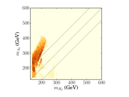
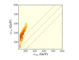
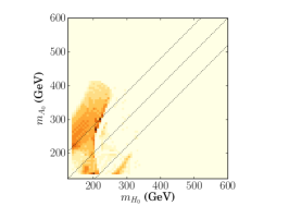
Figure 1: Heat maps with fixed $\tan(\beta)$, showing regions of first order EWPT ($0<x<0.11$ and $y\simeq 0$) in the alignment limit. The dotted lines correspond to $m_{A_{0}}=m_{H_{0}}$ and $m_{A_{0}}=m_{H_{0}}\pm m_{Z}$.

A uniform scan through a 10-dimensional space is computationally expensive; we must therefore make some simplifying assumptions. We take all parameters of the 2HDM to be real, setting $\text{Im}(\lambda_{5})=0$, $\text{Im}(\mu^{2}_{12})=0$. This eliminates extra CP violation in the model, which would be crucial for baryogenesis. However, the effect of these imaginary parts on the strength of the transition is expected to be negligible; the CP-violating phase must necessarily be small due to EDM constraints Inoue:2014nva ; Dorsch:2016nrg ; Chen:2017com .

Next, we reparametrise the model following Ref. Dorsch:2017nza , applying tree-level relations between the ${\overline{\mbox{\rm MS}}}$ parameters and physical quantities; accounting for (possibly sizeable) loop effects from vacuum renormalisation is left for future work. The masses of the CP-even scalars are denoted by $m_{h}=125\leavevmode\nobreak\ \mathrm{GeV}$ and $m_{H_{0}}$; that of the CP-odd scalar by $m_{A_{0}}$; and that of the charged scalar by $m_{H^{\pm}}$. We also employ two angles $\alpha$ and $\beta$: $\alpha$ parametrises mixing between the CP-even states, while $\beta$ is related to the ratio of the vevs $\tan(\beta)\equiv\frac{\nu_{2}}{\nu_{1}}$. Here, $\nu_{1}$ and $\nu_{2}$ are the vevs for $\phi_{1}$ and $\phi_{2}$, respectively, with $\nu^{2}_{1}+\nu^{2}_{2}=\nu^{2}$ and $\nu=246\leavevmode\nobreak\ \mathrm{GeV}$. Finally, there is the squared mass scale $M^{2}\equiv\mu^{2}(\tan(\beta)+1/\tan(\beta))$, where we treat $\mu^{2}\equiv-\mathrm{Re}\,\mu^{2}_{12}$ as an input parameter. The relations between the physical states and gauge eigenstates can be obtained from Ref. Dorsch:2017nza .

We also fix $m_{H^{\pm}}=m_{A_{0}}$, since EW precision tests require the mass of the charged Higgs to be roughly degenerate with either $H_{0}$ or $A_{0}$ Grimus:2007if ; Grimus:2008nb . Furthermore, we work in the alignment limit, setting $\cos(\beta-\alpha)=0$. In this limit, the CP-even scalar $h$ couples to SM particles exactly like the SM Higgs. We investigate relatively few values for $\tan(\beta)$, whereas we perform a more exhaustive scan in a three-dimensional parameter space spanned by $m_{H_{0}}$, $m_{A_{0}}$, and $\mu^{2}$. At each point, we require that tree-level stability and unitary constraints be satisfied; for details, see Ref. Gorda:2018hvi . Furthermore, for the scaling assumptions of DR to be valid, the tree-level mass parameters $\mu_{11}$, $\mu_{22}$ and $\mu_{12}$ should be comparable to the Debye mass $m_{D}\sim gT$ near the phase transition. This sets an upper bound for the input parameter $\mu\lesssim 200\leavevmode\nobreak\ \mathrm{GeV}$. Finally, we verify that in the effective theory the other doublet really is heavy near the phase transition, so it is justified to integrate it out.

IV Results

Following our scanning protocol outlined above, we fix $\tan(\beta)$ and scan in the two scalar masses $m_{H_{0}}$ and $m_{A_{0}}$ between $137.5$ and $562.5\leavevmode\nobreak\ \mathrm{GeV}$ at spacings of $6.25\leavevmode\nobreak\ \mathrm{GeV}$, a total of 4624 points. A dense scan in $\mu$ is then carried out for each pair, from 10 to 150 GeV at intervals of 2.5 GeV for a total of 56 values. In all, each of our fixed-$\tan(\beta)$ plots results from scanning approximately 260 000 points. The upper limit on $\mu$ is chosen to ensure that DR is valid, as explained above.

We first check whether each point is physical, according to our criteria. If so, we then perform DR for evenly-spaced temperatures between 80 and 200 GeV, at intervals of 20 GeV. This allows us to find the value of $x$ when $y=0$—on the critical line—by interpolation. We then use $x$ to characterise the phase transition. We take $0.0<x<0.11$ as an indicator of a first-order EWPT, the upper limit coming from previous lattice work.

Combining different values of $\mu$, we indicate the relative number of points with a first-order phase transition as a heat map in Fig. 1, for three separate values of $\tan(\beta)$. The majority of our points reside in the region $m_{A_{0}}>m_{H_{0}}+m_{Z}$, in accordance with Refs. Dorsch:2014qja ; Dorsch:2017nza (see, however, Refs. Basler:2016obg ; Basler:2017uxn ). In our framework, sufficiently strong interactions with the second doublet are necessary to bring $x$ down from its SM value of $x>0.11$. Although the relation between the 4D inputs and $x$ is complicated by the diagonalization, a mass hierarchy between $H_{0}$ and $A_{0}$ generically results in large portal couplings $\lambda_{3-5}$ and small values of $x$ in the upper region. However, at small $\tan(\beta)$ we also see a considerable number of points in regions where this does not hold.

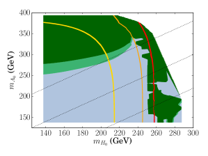
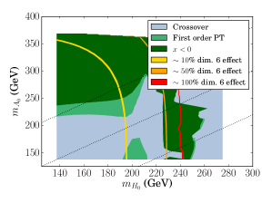
Figure 2: Slices with different values of $\mu$, $\mu=50$ GeV (top) and 75 GeV (bottom), and fixed $\tan(\beta)=2.0$. The validity of DR is estimated by showing the relative effect of the neglected six-dimensional operators $\mathcal{O}^{(6)}_{A,1}$, $\mathcal{O}^{(6)}_{A,2}$. The white regions are either unphysical or there is no transition. At large $m_{H_{0}}$ the effects of six-dimensional operators render the first DR step unreliable.

In Fig. 2, we show a breakdown of the heatmap plot with fixed $\tan(\beta)=2.0$ for two values of $\mu$. We include here an estimate of the effect of two of the neglected six-dimensional operators $\mathcal{O}^{(6)}_{A,1}$ and $\mathcal{O}^{(6)}_{A,2}$ produced when the superheavy scale is integrated out. Generally, decreasing values of $x$ correspond to increasing importance of six-dimensional terms: when the effect of these terms becomes large, DR breaks down. These plots also show how the lower first-order region disappears as $\mu$ increases.

We have found by explicit computation that the negative-$x$ region at large $m_{A_{0}}$ is due to the omission of the six-dimensional operator $\mathcal{O}^{(6)}_{B}$ in the last DR step that, although inversely proportional to the heavy doublet mass, obtains sizable contributions from the large couplings. We estimate its effect by computing the dominant tree-level diagram contributing to the operator coefficient (see Laine:1996ms and the Supplemental Material) and determining the two-loop effective potential in the final effective theory with this operator included (cf. Refs. Farakos:1994kx ; Kajantie:1995dw ). We stress, however, that the effective potential is only a tool for estimating errors from omitted six-dimensional operators; our results concerning the phase transition are obtained using the non-perturbative phase diagram of Kajantie:1995kf ; Kajantie:1996qd .

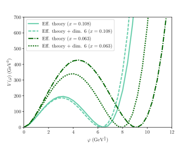
In Fig. 3, the effective potential is depicted at two values of $x$, both with and without the effects of the six-dimensional operator $\mathcal{O}^{(6)}_{B}$. The field $\varphi$ is the 3D background field, defined via $\langle\phi\rangle_{\text{3D}}=\frac{\varphi}{\sqrt{2}}\begin{pmatrix}0&1\end{pmatrix}^{\mathrm{T}}$ and related to 4D fields as described in the Supplemental Material. The figure demonstrates how at $x=0.108$—near the crossover boundary—the six-dimensional operator $\mathcal{O}^{(6)}_{B}$ has a negligible impact on the potential, while for $x=0.068$ (which corresponds to $\phi_{\mathrm{c}}/T_{\mathrm{c}}\approx 0.7$) the effect is already sizable, continuing to grow as $x$ decreases. Hence integrating out the heavier doublet is expected to be a valid approximation when the transition is of weakly first order, but becomes increasingly challenged near the strong transition limit of $x\lesssim 0.04$. While we expect our results to be qualitatively robust even there, reaching quantitatively accurate results for very small $x$ clearly calls for simulations with two dynamical doublets, which we leave for future work.

Figure 3: Two-loop effective potential in the final effective theory with the dominant six-dimensional operator $\mathcal{O}^{(6)}_{B}$ of the last DR step included, evaluated at the critical temperature. At small $x$, integrating out the second doublet causes significant error, as is seen from the shift in the potential minimum.

Experimental constraints on the 2HDM parameter space depend strongly on the way in which fermions couple to the Higgs doublets. With the exception of the top quark, other Yukawa couplings have little effect on our EWPT analysis, and we have still to indicate whether we are considering Type I (all quarks couple to $\phi_{2}$) or Type II (up-type quarks couple to $\phi_{2}$, down-type to $\phi_{1}$) 2HDM. The most stringent constraints come from flavour physics, where $B$-decays set the bound $m_{H^{\pm}}\gtrsim 580$ GeV for the charged Higgs mass in Type II Misiak:2017bgg . Assuming that $m_{H}^{\pm}$ is degenerate with $m_{A_{0}}$ in accordance with EW precision tests, this rules out our regions of first-order EWPT in Type II, but no such lower bound exists in Type I for $\tan\beta\geq 2$ Mahmoudi:2009zx ; Misiak:2017bgg .

Additional restrictions come from direct searches for neutral Higgses at the LHC Aad:2014vgg . For Type I, the $H_{0}\leavevmode\nobreak\ \rightarrow\leavevmode\nobreak\ \tau\tau$ cross section is suppressed by $\cot^{2}\beta$, and our choices of $\tan\beta$ are within current experimental bounds. Finally, we have verified that the mass range we scan in is allowed by measurements of the $h\rightarrow\gamma\gamma$ decay CMS:2015kwa , as well as the relatively recent search for $A_{0}\rightarrow Zh$ processes Aad:2015wra . Having not scanned in the hidden-Higgs region where constraints from charged-scalar searches become important Pierce:2007ut , we conclude that our first-order EWPT regions are currently not ruled out by experiments if a Type I 2HDM is assumed.

V Discussion

It is a shortcoming of present-day particle cosmology that it is still impossible to reliably determine the nature and strength of the EWPT for a given BSM scenario. This information would be valuable not only for EWBG, but also for gravitational wave physics, as a first-order EWPT would leave an imprint in the sensitivity range of the LISA mission and other proposed gravitational-wave detectors Caprini:2015zlo .

We have taken a step towards remedying the situation by studying the mapping of the phase diagram of one viable BSM theory, the 2HDM. Our results concern the EWPT in the alignment limit $\cos(\beta-\alpha)$ = 0. Our work so far supports the idea that the primary signature of a first order transition in this theory is indeed $m_{A_{0}}>m_{H_{0}}+m_{Z}$, as suggested by Refs. Dorsch:2014qja ; Dorsch:2017nza .

The techniques discussed in this paper can be applied, with suitable modifications, to a host of other models where a substantial region of parameter space can be mapped onto the three-dimensional theory of the minimal Standard Model. In the future, our aim is to perform a thorough comparison of perturbative and non-perturbative results in the 2HDM by keeping both doublets dynamical in the effective theory. Similar projects to study the EWPT and benchmark the accuracy of perturbation theory are already underway in the Standard Model augmented by a real singlet singlet_scans or triplet field Niemi:2018asa ; the EWPT has been perturbatively analysed for the former in Refs. Beniwal:2017eik ; Chen:2017qcz , and for the latter in Ref. Patel:2012pi .

Supplemental Material

Appendix A Dimensional reduction of 2HDM

In this Supplemental Material we collect the matching relations between the full four-dimensional theory and effective theories. A detailed derivation can be found in Ref. Gorda:2018hvi .

A.1 Three-dimensional effective theories

We denote the fields of the effective theories with the same symbols as those of the four-dimensional theory, even though their normalisation is different and will affect the mapping between full and effective theories. These normalisations between 4D and 3D fields have been listed below.

The schematic form of classical Lagrangian density of the effective theory was given in Eq. (4) of the main paper. The temporal part reads

$$\mathcal{L}^{(3)}_{\text{temporal}}=\frac{1}{2}(D_{r}A^{a}_{0})^{2}+\frac{1}{2}m_{D}^{2}A^{a}_{0}A^{a}_{0}+\frac{1}{2}(\partial_{r}B_{0})^{2}+\frac{1}{2}m_{D}^{\prime 2}B_{0}^{2}+\frac{1}{4}\kappa_{1}(A^{a}_{0}A^{a}_{0})^{2}+\frac{1}{4}\kappa_{2}B_{0}^{4}\\ +\frac{1}{4}\kappa_{3}A^{a}_{0}A^{a}_{0}B_{0}^{2}+h_{1}\phi^{\dagger}_{1}\phi_{1}A^{a}_{0}A^{a}_{0}+h_{2}\phi^{\dagger}_{1}\phi_{1}B_{0}^{2}+h_{3}B_{0}\phi^{\dagger}_{1}\vec{A}_{0}\cdot\vec{\tau}\phi_{1}+h_{4}\phi^{\dagger}_{2}\phi_{2}A^{a}_{0}A^{a}_{0}\\ +h_{5}\phi^{\dagger}_{2}\phi_{2}B_{0}^{2}+h_{6}B_{0}\phi^{\dagger}_{2}\vec{A}_{0}\cdot\vec{\tau}\phi_{2}+\frac{1}{2}(\partial_{r}C^{\alpha}_{0})^{2}+\frac{1}{2}m_{D}^{\prime\prime 2}C^{\alpha}_{0}C^{\alpha}_{0}+\omega_{3}C^{\alpha}_{0}C^{\alpha}_{0}\phi^{\dagger}_{2}\phi_{2}.$$ (7)

Here the covariant derivative of an isospin triplet reads $D_{r}A^{a}_{0}=\partial_{r}A^{a}_{0}+g_{3}\epsilon^{abc}A^{b}_{r}A^{c}_{0}$, and for the temporal gluon $C^{\alpha}_{0}$ ordinary derivative is used instead of covariant derivative as gluons are discarded for only contributing at a higher order Brauner:2016fla .

After the heavy temporal scalars have been integrated out, their effects are encoded by the parameters and fields of a new theory where the parameters are denoted with a bar as $\bar{g}_{3},{\bar{g}^{\prime}}_{3},\bar{\mu}^{2}_{11,3}$ etc. In this theory, the phase transition takes place close to a point where the mass matrix has zero eigenvalue, and then generically in the diagonal basis the other mass parameter is heavy. By performing a unitary transformation, one can diagonalise the scalar potential. Denoting $\Omega\equiv\;\sqrt{(\bar{\mu}^{2}_{11,3}-\bar{\mu}^{2}_{22,3})^{2}+4\bar{\mu}^{2*}_{12,3}\bar{\mu}^{2}_{12,3}}$, this transformation reads

$$\begin{pmatrix}\phi_{1}\\ \phi_{2}\end{pmatrix}\equiv\begin{pmatrix}\alpha&\beta\\ \gamma&\delta\end{pmatrix}\begin{pmatrix}\theta\\ \phi\end{pmatrix},$$ (8)

where

$$\alpha \equiv\frac{2}{\sqrt{4+\left|\frac{(\bar{\mu}^{2}_{22,3}-\bar{\mu}^{2}_{11,3})+\Omega}{\bar{\mu}^{2*}_{12,3}}\right|^{2}}}, \beta \equiv\;\frac{(\bar{\mu}^{2}_{11,3}-\bar{\mu}^{2}_{22,3}-\Omega^{*})}{\bar{\mu}^{2}_{12,3}\sqrt{4+\left|\frac{(\bar{\mu}^{2}_{22,3}-\bar{\mu}^{2}_{11,3})+\Omega}{\bar{\mu}^{2*}_{12,3}}\right|^{2}}}$$

$$\gamma \equiv\frac{2}{\sqrt{4+\left|\frac{-(\bar{\mu}^{2}_{22,3}-\bar{\mu}^{2}_{11,3})+\Omega}{\bar{\mu}^{2*}_{12,3}}\right|^{2}}}, \delta \equiv\;\frac{(\bar{\mu}^{2}_{11,3}-\bar{\mu}^{2}_{22,3}+\Omega^{*})}{\bar{\mu}^{2}_{12,3}\sqrt{4+\left|\frac{-(\bar{\mu}^{2}_{22,3}-\bar{\mu}^{2}_{11,3})+\Omega}{\bar{\mu}^{2*}_{12,3}}\right|^{2}}}.$$ (9)

The mass parameters in the diagonal basis read

$$\widetilde{\mu}^{2}_{\phi} =\frac{1}{2}(\bar{\mu}^{2}_{11,3}+\bar{\mu}^{2}_{22,3}-\Omega), \widetilde{\mu}^{2}_{\theta} =\frac{1}{2}(\bar{\mu}^{2}_{11,3}+\bar{\mu}^{2}_{22,3}+\Omega).$$ (10)

Generally $\widetilde{\mu}^{2}_{\theta}$ is heavy when $\widetilde{\mu}^{2}_{\phi}$ is light, and therefore the field $\theta$ can be integrated out. The scalar self-couplings in the diagonal basis are given by

$$\begin{pmatrix}\widetilde{\lambda}_{1}\\ \widetilde{\lambda}_{2}\\ \widetilde{\lambda}_{3}\\ \widetilde{\lambda}_{4}\\ \widetilde{\lambda}_{5}/2\\ \widetilde{\lambda}_{6}\\ \widetilde{\lambda}_{7}\end{pmatrix}=M\cdot\begin{pmatrix}\bar{\lambda}_{1,3}\\ \bar{\lambda}_{2,3}\\ \bar{\lambda}_{3,3}\\ \bar{\lambda}_{4,3}\\ \bar{\lambda}_{5,3}/2\\ \bar{\lambda}^{*}_{5,3}/2\end{pmatrix},$$ (11)

where

$$M\equiv\begin{pmatrix}|\beta|^{4}&|\delta|^{4}&|\beta|^{2}|\delta|^{2}&|\beta|^{2}|\delta|^{2}&(\beta^{*}\delta)^{2}&(\beta\delta^{*})^{2}\\ |\alpha|^{4}&|\gamma|^{4}&|\alpha|^{2}|\gamma|^{2}&|\alpha|^{2}|\gamma|^{2}&(\alpha^{*}\gamma)^{2}&(\alpha\gamma^{*})^{2}\\ 2|\alpha|^{2}|\beta|^{2}&2|\gamma|^{2}|\delta|^{2}&|\alpha|^{2}|\delta|^{2}+|\beta|^{2}|\gamma|^{2}&2\operatorname{Re}(\alpha\beta^{*}\gamma^{*}\delta)&2\alpha^{*}\beta^{*}\gamma\delta&2\alpha\beta\gamma^{*}\delta^{*}\\ 2|\alpha|^{2}|\beta|^{2}&2|\gamma|^{2}|\delta|^{2}&2\operatorname{Re}(\alpha\beta^{*}\gamma^{*}\delta)&|\alpha|^{2}|\delta|^{2}+|\beta|^{2}|\gamma|^{2}&2\alpha^{*}\beta^{*}\gamma\delta&2\alpha\beta\gamma^{*}\delta^{*}\\ (\alpha\beta^{*})^{2}&(\gamma\delta^{*})^{2}&\alpha\beta^{*}\gamma\delta^{*}&\alpha\beta^{*}\gamma\delta^{*}&(\beta^{*}\gamma)^{2}&(\alpha\delta^{*})^{2}\\ 2|\beta|^{2}\alpha\beta^{*}&2|\delta|^{2}\gamma\delta^{*}&\beta^{*}\delta^{*}(\beta\gamma+\alpha\delta)&\beta^{*}\delta^{*}(\beta\gamma+\alpha\delta)&2\beta^{*}\gamma\beta^{*}\delta&2\alpha\beta\delta^{*}\delta^{*}\\ 2|\alpha|^{2}\alpha^{*}\beta&2|\gamma|^{2}\gamma^{*}\delta&\alpha^{*}\gamma^{*}(\beta\gamma+\alpha\delta)&\alpha^{*}\gamma^{*}(\beta\gamma+\alpha\delta)&2\alpha^{*}\gamma\alpha^{*}\delta&2\alpha\beta\gamma^{*}\gamma^{*}\\ \end{pmatrix}.$$ (12)

The scalar potential in the diagonal basis reads

$$V(\phi,\theta)=\widetilde{\mu}^{2}_{\phi}\phi^{\dagger}\phi+\widetilde{\mu}^{2}_{\theta}\theta^{\dagger}\theta+\widetilde{\lambda}_{1}(\phi^{\dagger}\phi)^{2}+\widetilde{\lambda}_{2}(\theta^{\dagger}\theta)^{2}+\widetilde{\lambda}_{3}(\phi^{\dagger}\phi)(\theta^{\dagger}\theta)+\widetilde{\lambda}_{4}(\phi^{\dagger}\theta)(\theta^{\dagger}\phi)\\ +\frac{\widetilde{\lambda}_{5}}{2}(\phi^{\dagger}\theta)^{2}+\frac{\widetilde{\lambda}^{*}_{5}}{2}(\theta^{\dagger}\phi)^{2}+\widetilde{\lambda}_{6}(\phi^{\dagger}\phi)(\phi^{\dagger}\theta)+\widetilde{\lambda}^{*}_{6}(\phi^{\dagger}\phi)(\theta^{\dagger}\phi)+\widetilde{\lambda}_{7}(\theta^{\dagger}\theta)(\theta^{\dagger}\phi)+\widetilde{\lambda}^{*}_{7}(\theta^{\dagger}\theta)(\phi^{\dagger}\theta),$$ (13)

where $\phi$ and $\theta$ are light and heavy fields, respectively.

When the heavy doublet $\theta$ has been integrated out, the final effective theory is same as in that of the SM, as given in Eq. (6) of the main paper.

A.2 Matching relations and normalisations of fields

Our calculations are carried out in the ${\overline{\mbox{\rm MS}}}$ scheme. We use the following notation:

$$N_{d} =2,$$

$$L_{b} \equiv 2\ln\left(\frac{\Lambda}{T}\right)-2[\ln(4\pi)-\gamma],$$ (14)

$$L_{f} \equiv L_{b}+4\ln 2,$$

$$c \equiv\frac{1}{2}\left(\ln\left(\frac{8\pi}{9}\right)+\frac{\zeta^{\prime}(2)}{\zeta(2)}-2\gamma\right),$$

where $\Lambda$ is the renormalisation scale of the 4D theory and $\gamma$ is the Euler-Mascheroni constant.

The normalisations relating three- and four-dimensional fields read

$$A_{\text{3D},0}^{2} =\frac{A_{\text{4D},0}^{2}}{T}\left\{1+\frac{g^{2}}{(4\pi)^{2}}\left[\frac{N_{d}-26}{6}L_{b}+\frac{1}{3}(8+N_{d})+\frac{4N_{f}}{3}(L_{f}-1)\right]\right\},$$

$$A_{\text{3D},r}^{2} =\frac{A_{\text{4D},r}^{2}}{T}\left[1+\frac{g^{2}}{(4\pi)^{2}}\left(\frac{N_{d}-26}{6}L_{b}-\frac{2}{3}+\frac{4N_{f}}{3}L_{f}\right)\right],$$

$$B_{\text{3D},0}^{2} =\frac{B_{\text{4D},0}^{2}}{T}\left\{1+\frac{g^{\prime 2}}{(4\pi)^{2}}\left[N_{d}\left(\frac{L_{b}}{6}+\frac{1}{3}\right)+\frac{20N_{f}}{9}(L_{f}-1)\right]\right\},$$

$$B_{\text{3D},r}^{2} =\frac{B_{\text{4D},r}^{2}}{T}\left[1+\frac{g^{\prime 2}}{(4\pi)^{2}}\left(N_{d}\frac{L_{b}}{6}+\frac{20N_{f}}{9}L_{f}\right)\right],$$ (15)

$$\left(\phi^{\dagger}_{1}\phi_{1}\right)_{\text{3D}} =\frac{\left(\phi^{\dagger}_{1}\phi_{1}\right)_{\text{4D}}}{T}\left[1-\frac{1}{(4\pi)^{2}}\left(\frac{3}{4}(3g^{2}+{g^{\prime}}^{2})L_{b}\right)\right],$$

$$\left(\phi^{\dagger}_{2}\phi_{2}\right)_{\text{3D}} =\frac{\left(\phi^{\dagger}_{2}\phi_{2}\right)_{\text{4D}}}{T}\left[1-\frac{1}{(4\pi)^{2}}\left(\frac{3}{4}(3g^{2}+{g^{\prime}}^{2})L_{b}-3g^{2}_{Y}L_{f}\right)\right],$$

$$\left(\phi^{\dagger}_{1}\phi_{2}\right)_{\text{3D}} =\frac{\left(\phi^{\dagger}_{1}\phi_{2}\right)_{\text{4D}}}{T}\left[1-\frac{1}{(4\pi)^{2}}\left(\frac{3}{4}(3g^{2}+{g^{\prime}}^{2})L_{b}-\frac{3}{2}g^{2}_{Y}L_{f}\right)\right].$$

For dimensional reduction, the required ingredients include matching relations between the 4D and 3D theories, one-loop $\beta$ functions (to make the matching relations renormalisation scale independent) and finally the relations between $\overline{\rm MS}$-parameters and physical quantities.

We use the tree-level relations, despite the fact that for consistent $O(g^{4})$ accuracy one should use the one-loop corrected relations. This would require performing one-loop vacuum renormalisation of the physical quantities. This is a non-trivial task, and is left for the future. In the special case of the inert doublet model, the one-loop vacuum renormalisation can be found in Ref. Laine:2017hdk . Below we list all needed matching relations, while $\beta$ functions and relations of ${\overline{\mbox{\rm MS}}}$-parameters and physical quantities can be found in Ref. Gorda:2018hvi with detailed derivations and explicit, step-by-step intermediate results.

A.2.1 Integration over superheavy scale

A full $O(g^{4})$-accurate dimensional reduction requires the evaluation of the mass parameters at two-loop and couplings at one-loop order. The results are listed below.

$$m_{D}^{2}={} g^{2}T^{2}\bigg{(}\frac{4+N_{d}}{6}+\frac{N_{f}}{3}\bigg{)},$$ (16)

$$m^{\prime 2}_{D}={} g^{\prime 2}T^{2}\bigg{(}\frac{N_{d}}{6}+\frac{5N_{f}}{9}\bigg{)},$$ (17)

$$m^{\prime\prime 2}_{D}={} g^{2}_{s}T^{2}\bigg{(}1+\frac{N_{f}}{6}\bigg{)},$$ (18)

$$g_{3}^{2}={} g^{2}(\Lambda)T\bigg{[}1+\frac{g^{2}}{(4\pi)^{2}}\bigg{(}\frac{44-N_{d}}{6}L_{b}+\frac{2}{3}-\frac{4N_{f}}{3}L_{f}\bigg{)}\bigg{]},$$ (19)

$$g^{\prime 2}_{3}={} g^{\prime 2}(\Lambda)T\bigg{[}1-\frac{g^{\prime 2}}{(4\pi)^{2}}\bigg{(}\frac{N_{d}}{6}L_{b}+\frac{20N_{f}}{9}L_{f}\bigg{)}\bigg{]},$$ (20)

$$\kappa_{1}={} T\frac{g^{4}}{16\pi^{2}}\frac{16+N_{d}-4N_{f}}{3},$$ (21)

$$\kappa_{2}={} T\frac{g^{\prime 4}}{16\pi^{2}}\bigg{(}\frac{N_{d}}{3}-\frac{380}{81}N_{f}\bigg{)},$$ (22)

$$\kappa_{3}={} T\frac{g^{2}g^{\prime 2}}{16\pi^{2}}\bigg{(}2N_{d}-\frac{8}{3}N_{f}\bigg{)},$$ (23)

$$h_{1}={} \frac{g^{2}(\Lambda)T}{4}\bigg{(}1+\frac{1}{(4\pi)^{2}}\bigg{\{}\bigg{[}\frac{44-N_{d}}{6}L_{b}+\frac{53}{6}-\frac{N_{d}}{3}-\frac{4N_{f}}{3}(L_{f}-1)\bigg{]}g^{2}+\frac{g^{\prime 2}}{2}$$

$$\quad\quad\quad\quad\quad\quad\quad\quad\quad+12\lambda_{1}+2(2\lambda_{3}+\lambda_{4})\bigg{\}}\bigg{)},$$ (24)

$$h_{2}={} \frac{g^{\prime 2}(\Lambda)T}{4}\bigg{(}1+\frac{1}{(4\pi)^{2}}\bigg{\{}\frac{3g^{2}}{2}+\bigg{[}\frac{1}{2}-\frac{N_{d}}{6}\Big{(}2+L_{b}\Big{)}-\frac{20N_{f}}{9}(L_{f}-1)\bigg{]}g^{\prime 2}$$

$$\quad\quad\quad\quad\quad\quad\quad\quad\quad+12\lambda_{1}+2(2\lambda_{3}+\lambda_{4})\bigg{\}}\bigg{)},$$ (25)

$$h_{3}={} \frac{g(\Lambda)g^{\prime}(\Lambda)T}{2}\bigg{\{}1+\frac{1}{(4\pi)^{2}}\bigg{[}-\frac{5+N_{d}}{6}g^{2}+\frac{3-N_{d}}{6}g^{\prime 2}+L_{b}\bigg{(}\frac{44-N_{d}}{12}g^{2}-\frac{N_{d}}{12}g^{\prime 2}\bigg{)}$$

$$-N_{f}(L_{f}-1)\bigg{(}\frac{2}{3}g^{2}+\frac{10}{9}g^{\prime 2}\bigg{)}+4\lambda_{1}+2\lambda_{4}\bigg{]}\bigg{\}},$$ (26)

$$h_{4}={} \frac{g^{2}(\Lambda)T}{4}\bigg{(}1+\frac{1}{(4\pi)^{2}}\bigg{\{}\bigg{[}\frac{44-N_{d}}{6}L_{b}+\frac{53}{6}-\frac{N_{d}}{3}-\frac{4N_{f}}{3}(L_{f}-1)\bigg{]}g^{2}+\frac{g^{\prime 2}}{2}-6g_{Y}^{2}$$ (27)

$$\quad\quad\quad\quad\quad\quad\quad\quad\quad+12\lambda_{2}+2(2\lambda_{3}+\lambda_{4})\bigg{\}}\bigg{)},$$ (28)

$$h_{5}={} \frac{g^{\prime 2}(\Lambda)T}{4}\bigg{(}1+\frac{1}{(4\pi)^{2}}\bigg{\{}\frac{3g^{2}}{2}+\bigg{[}\frac{1}{2}-\frac{N_{d}}{6}\Big{(}2+L_{b}\Big{)}-\frac{20N_{f}}{9}(L_{f}-1)\bigg{]}g^{\prime 2}-\frac{34}{3}g_{Y}^{2}$$

$$\quad\quad\quad\quad\quad\quad\quad\quad\quad+12\lambda_{2}+2(2\lambda_{3}+\lambda_{4})\bigg{\}}\bigg{)},$$ (29)

$$h_{6}={} \frac{g(\Lambda)g^{\prime}(\Lambda)T}{2}\bigg{\{}1+\frac{1}{(4\pi)^{2}}\bigg{[}-\frac{5+N_{d}}{6}g^{2}+\frac{3-N_{d}}{6}g^{\prime 2}+L_{b}\bigg{(}\frac{44-N_{d}}{12}g^{2}-\frac{N_{d}}{12}g^{\prime 2}\bigg{)}$$

$$-N_{f}(L_{f}-1)\bigg{(}\frac{2}{3}g^{2}+\frac{10}{9}g^{\prime 2}\bigg{)}+2g_{Y}^{2}+4\lambda_{2}+2\lambda_{4}\bigg{]}\bigg{\}},$$ (30)

$$\omega_{3}={} -\frac{2T}{16\pi^{2}}g^{2}_{s}g^{2}_{Y},$$ (31)

$$\lambda_{1,3}={} T\Bigg{\{}\lambda_{1}(\Lambda)+\frac{1}{(4\pi)^{2}}\bigg{[}\frac{1}{8}\Big{(}3g^{4}+{g^{\prime}}^{4}+2g^{2}{g^{\prime}}^{2}\Big{)}$$

$$-L_{b}\bigg{(}\frac{3}{16}\Big{(}3g^{4}+{g^{\prime}}^{4}+2g^{2}{g^{\prime}}^{2}\Big{)}+\lambda^{2}_{3}+\lambda_{3}\lambda_{4}+\frac{1}{2}\lambda^{2}_{4}+\frac{1}{2}|\lambda_{5}|^{2}-\frac{3}{2}\Big{(}3g^{2}+{g^{\prime}}^{2}-8\lambda_{1}\Big{)}\lambda_{1}\bigg{)}\bigg{]}\Bigg{\}},$$ (32)

$$\lambda_{2,3}={} T\Bigg{\{}\lambda_{2}(\Lambda)+\frac{1}{(4\pi)^{2}}\bigg{[}\frac{1}{8}\Big{(}3g^{4}+{g^{\prime}}^{4}+2g^{2}{g^{\prime}}^{2}\Big{)}+3L_{f}\Big{(}g^{4}_{Y}-2\lambda_{2}g^{2}_{Y}\Big{)}$$

$$-L_{b}\bigg{(}\frac{3}{16}\Big{(}3g^{4}+{g^{\prime}}^{4}+2g^{2}{g^{\prime}}^{2}\Big{)}+\lambda^{2}_{3}+\lambda_{3}\lambda_{4}+\frac{1}{2}\lambda^{2}_{4}+\frac{1}{2}|\lambda_{5}|^{2}-\frac{3}{2}\Big{(}3g^{2}+{g^{\prime}}^{2}-8\lambda_{2}\Big{)}\lambda_{2}\bigg{)}\bigg{]}\Bigg{\}},$$ (33)

$$\lambda_{3,3}={} T\Bigg{\{}\lambda_{3}(\Lambda)+\frac{1}{(4\pi)^{2}}\bigg{[}\frac{1}{4}\Big{(}3g^{4}+{g^{\prime}}^{4}-2g^{2}{g^{\prime}}^{2}\Big{)}-3L_{f}\lambda_{3}g^{2}_{Y}$$

$$-L_{b}\bigg{(}\frac{3}{8}\Big{(}3g^{4}+{g^{\prime}}^{4}-2g^{2}{g^{\prime}}^{2}\Big{)}+2(\lambda_{1}+\lambda_{2})(3\lambda_{3}+\lambda_{4})+2\lambda^{2}_{3}+\lambda^{2}_{4}+|\lambda_{5}|^{2}-\frac{3}{2}\Big{(}3g^{2}+{g^{\prime}}^{2}\Big{)}\lambda_{3}\bigg{)}\bigg{]}\Bigg{\}},$$ (34)

$$\lambda_{4,3}={} T\Bigg{\{}\lambda_{4}(\Lambda)+\frac{1}{(4\pi)^{2}}\bigg{[}g^{2}{g^{\prime}}^{2}-3L_{f}\lambda_{4}g^{2}_{Y}$$

$$-L_{b}\bigg{(}\frac{3}{2}g^{2}{g^{\prime}}^{2}+2(\lambda_{1}+\lambda_{2})\lambda_{4}+2\lambda^{2}_{4}+4\lambda_{3}\lambda_{4}+4|\lambda_{5}|^{2}-\frac{3}{2}\Big{(}3g^{2}+{g^{\prime}}^{2}\Big{)}\lambda_{4}\bigg{)}\bigg{]}\Bigg{\}}$$ (35)

$$\text{and}\quad\lambda_{5,3}={} T\Bigg{\{}\lambda_{5}(\Lambda)+\frac{1}{(4\pi)^{2}}\bigg{[}-3L_{f}\lambda_{5}g^{2}_{Y}-L_{b}\bigg{(}2(\lambda_{1}+\lambda_{2}+2\lambda_{3}+3\lambda_{4})\lambda_{5}-\frac{3}{2}\Big{(}3g^{2}+{g^{\prime}}^{2}\Big{)}\lambda_{5}\bigg{)}\bigg{]}\Bigg{\}}.$$ (36)

These relations have been calculated previously in Ref. Losada:1996ju , with the restriction of $\lambda_{5}$ being real rather than complex. We have corrected two minor errors in the expressions for $\lambda_{4,3}$ and $\lambda_{5,3}$ for the terms involving $\lambda_{5}$.

In the Standard Model, the $O(g^{4})$ result for the 3D scalar mass parameter reads:

$$\Big{(}\mu^{2}_{22,3}\Big{)}_{\text{SM}}= \mu^{2}_{22}(\Lambda)+\frac{T^{2}}{16}\Big{(}3g^{2}(\Lambda)+{g^{\prime}}^{2}(\Lambda)+4g^{2}_{Y}(\Lambda)+8\lambda_{2}(\Lambda)\Big{)}$$

$$+\frac{1}{16\pi^{2}}\bigg{\{}\mu^{2}_{22}\bigg{(}\Big{(}\frac{3}{4}(3g^{2}+{g^{\prime}}^{2})-6\lambda_{2}\Big{)}L_{b}-3g^{2}_{Y}L_{f}\bigg{)}$$

$$+T^{2}\bigg{(}\frac{167}{96}g^{4}+\frac{1}{288}{g^{\prime}}^{4}-\frac{3}{16}g^{2}{g^{\prime}}^{2}+\frac{1}{4}\lambda_{2}(3g^{2}+{g^{\prime}}^{2})$$

$$+L_{b}\Big{(}\frac{17}{16}g^{4}-\frac{5}{48}{g^{\prime}}^{4}-\frac{3}{16}g^{2}{g^{\prime}}^{2}+\frac{3}{4}\lambda_{2}(3g^{2}+{g^{\prime}}^{2})-6\lambda^{2}_{2}\Big{)}$$

$$+\frac{1}{T^{2}}\Big{(}c+\ln(\frac{3T}{\Lambda_{\text{3D}}})\Big{)}\Big{(}\frac{39}{16}g^{4}_{3}+12g^{2}_{3}h_{4}-6h^{2}_{4}+9g^{2}_{3}\lambda_{2,3}-12\lambda^{2}_{2,3}$$

$$-\frac{5}{16}{g^{\prime}}^{4}_{3}-\frac{9}{8}g^{2}_{3}{g^{\prime}}^{2}_{3}-2h^{2}_{5}-3h^{2}_{6}+3{g^{\prime}}^{2}_{3}\lambda_{2,3}\Big{)}$$

$$-g^{2}_{Y}\Big{(}\frac{3}{16}g^{2}+\frac{11}{48}{g^{\prime}}^{2}+2g^{2}_{s}\Big{)}+(\frac{1}{12}g^{4}+\frac{5}{108}{g^{\prime}}^{4})N_{f}$$

$$+L_{f}\Big{(}g^{2}_{Y}\Big{(}\frac{9}{16}g^{2}+\frac{17}{48}{g^{\prime}}^{2}+2g^{2}_{s}-3\lambda_{2}\Big{)}+\frac{3}{8}g^{4}_{Y}-(\frac{1}{4}g^{4}+\frac{5}{36}{g^{\prime}}^{4})N_{f}\Big{)}$$

$$+\ln(2)\Big{(}g^{2}_{Y}\Big{(}-\frac{21}{8}g^{2}-\frac{47}{72}{g^{\prime}}^{2}+\frac{8}{3}g^{2}_{s}+9\lambda_{2}\Big{)}-\frac{3}{2}g^{4}_{Y}+(\frac{3}{2}g^{4}+\frac{5}{6}{g^{\prime}}^{4})N_{f}\Big{)}\bigg{)}\bigg{\}}.$$ (37)

This result can be found also in Ref. Kajantie:1995dw , apart from the two-loop contributions involving ${g^{\prime}}$, as in that paper these were assumed to scale as ${g^{\prime}}\sim g^{\frac{3}{2}}$.

In the 2HDM, the 3D scalar mass parameters read:

$$\Big{(}\mu^{2}_{22,3}\Big{)}_{\text{2HDM}}= \Big{(}\mu^{2}_{22,3}\Big{)}_{\text{SM}}+\frac{T^{2}}{12}\Big{(}2\lambda_{3}(\Lambda)+\lambda_{4}(\Lambda)\Big{)}$$

$$+\frac{1}{16\pi^{2}}\bigg{\{}\mu^{2}_{11}\Big{(}-L_{b}(2\lambda_{3}+\lambda_{4})\Big{)}$$

$$+T^{2}\bigg{(}\frac{5}{48}g^{4}+\frac{5}{144}{g^{\prime}}^{4}+\frac{1}{24}(3g^{2}+{g^{\prime}}^{2})(2\lambda_{3}+\lambda_{4})$$

$$+\frac{1}{T^{2}}\Big{(}c+\ln\big{(}\frac{3T}{\Lambda_{\text{3D}}}\big{)}\Big{)}\Big{(}-\frac{1}{8}(3g^{4}_{3}+{g^{\prime}}^{4}_{3})+\frac{1}{2}(3g^{2}_{3}+{g^{\prime}}^{2}_{3})(2\lambda_{3,3}+\lambda_{4,3})$$

$$-2(\lambda^{2}_{3,3}+\lambda_{3,3}\lambda_{4,3}+\lambda^{2}_{4,3})-3|\lambda_{5,3}|^{2}\Big{)}$$

$$+L_{b}\Big{(}-\frac{7}{32}g^{4}-\frac{7}{96}{g^{\prime}}^{4}-\frac{1}{2}(\lambda_{1}+\lambda_{2})(2\lambda_{3}+\lambda_{4})$$

$$-\frac{5}{6}\lambda^{2}_{3}-\frac{7}{12}\lambda^{2}_{4}-\frac{5}{6}\lambda_{3}\lambda_{4}-\frac{3}{4}|\lambda_{5}|^{2}+\frac{1}{8}(3g^{2}+{g^{\prime}}^{2})\big{(}2\lambda_{3}+\lambda_{4}\big{)}\Big{)}$$

$$+\Big{(}-\frac{1}{4}g^{2}_{Y}\big{(}2\lambda_{3}+\lambda_{4}\big{)}\Big{)}L_{f}\bigg{)}\bigg{\}},$$

and

$$\mu^{2}_{11,3}= \mu^{2}_{11}(\Lambda)+\frac{T^{2}}{16}\Big{(}3g^{2}(\Lambda)+{g^{\prime}}^{2}(\Lambda)+8\lambda_{1}(\Lambda)+\frac{4}{3}\Big{(}2\lambda_{3}(\Lambda)+\lambda_{4}(\Lambda)\Big{)}\Big{)}$$

$$+\frac{1}{16\pi^{2}}\bigg{\{}L_{b}\bigg{(}\Big{(}\frac{3}{4}(3g^{2}+{g^{\prime}}^{2})-6\lambda_{1}\Big{)}\mu^{2}_{11}-(2\lambda_{3}+\lambda_{4})\mu^{2}_{22}\bigg{)}$$

$$+T^{2}\bigg{(}\frac{59}{32}g^{4}+\frac{11}{288}{g^{\prime}}^{4}-\frac{3}{16}g^{2}{g^{\prime}}^{2}+\frac{1}{4}\lambda_{1}(3g^{2}+{g^{\prime}}^{2})+\frac{1}{24}(3g^{2}+{g^{\prime}}^{2})(2\lambda_{3}+\lambda_{4})$$

$$+L_{b}\Big{(}\frac{27}{32}g^{4}-\frac{17}{96}{g^{\prime}}^{4}-\frac{3}{16}g^{2}{g^{\prime}}^{2}+\frac{1}{8}(3g^{2}+{g^{\prime}}^{2})(6\lambda_{1}+2\lambda_{3}+\lambda_{4})-\frac{1}{2}(\lambda_{1}+\lambda_{2})(2\lambda_{3}+\lambda_{4})$$

$$-6\lambda^{2}_{1}-\frac{5}{6}\lambda^{2}_{3}-\frac{5}{6}\lambda_{3}\lambda_{4}-\frac{7}{12}\lambda^{2}_{4}-\frac{3}{4}|\lambda_{5}|^{2}\Big{)}$$

$$+\frac{1}{T^{2}}\Big{(}c+\ln(\frac{3T}{\Lambda_{\text{3D}}})\Big{)}\Big{(}\frac{33}{16}g^{4}_{3}+12g^{2}_{3}h_{1}-6h^{2}_{1}+9g^{2}_{3}\lambda_{1,3}-12\lambda^{2}_{1,3}$$

$$-\frac{7}{16}{g^{\prime}}^{4}_{3}-\frac{9}{8}g^{2}_{3}{g^{\prime}}^{2}_{3}-2h^{2}_{2}-3h^{2}_{3}+3{g^{\prime}}^{2}_{3}\lambda_{1,3}+\frac{1}{2}(3g^{2}_{3}+{g^{\prime}}^{2}_{3})(2\lambda_{3,3}+\lambda_{4,3})$$

$$-2(\lambda^{2}_{3,3}+\lambda_{3,3}\lambda_{4,3}+\lambda^{2}_{4,3})-3|\lambda_{5,3}|^{2}\Big{)}$$

$$+(\frac{1}{12}g^{4}+\frac{5}{108}{g^{\prime}}^{4})N_{f}+L_{f}\Big{(}-\frac{1}{4}g^{2}_{Y}(2\lambda_{3}+\lambda_{4})-(\frac{1}{4}g^{4}+\frac{5}{36}{g^{\prime}}^{4})N_{f}\Big{)}$$

$$+\ln(2)\Big{(}\frac{3}{2}g^{2}_{Y}\Big{(}2\lambda_{3}+\lambda_{4}\Big{)}+(\frac{3}{2}g^{4}+\frac{5}{6}{g^{\prime}}^{4})N_{f}\Big{)}\bigg{)}\bigg{\}},$$ (38)

and finally

$$\mu^{2}_{12,3}=\mu^{2}_{12}(\Lambda)+\frac{1}{16\pi^{2}}\bigg{\{}L_{b}\bigg{(}\Big{(}\frac{3}{4}(3g^{2}+{g^{\prime}}^{2})-\lambda_{3}-2\lambda_{4}\Big{)}\mu^{2}_{12}-3\lambda_{5}\mu^{2*}_{12}\bigg{)}-\frac{3}{2}g^{2}_{Y}\mu^{2}_{12}L_{f}\bigg{\}}.$$ (39)

We emphasise that all matching relations in the first step of DR are independent of the four-dimensional theory renormalisation scale $\Lambda$ to the order we consider here, which can be seen by applying the $\beta$ functions to the tree-level terms. This serves as a crosscheck of the correctness of our calculation. In practice, we fix $\Lambda=4\pi e^{-\gamma}T\approx 7T$, and have verified that the choice of $\Lambda$ has negligible effect on our results.

These relations for the two-loop mass parameters have been calculated previously in Ref. Andersen:1998br , under the assumption of $\lambda_{5}$ being real (see also Ref. Losada:1998at ). However, in Ref. Andersen:1998br there are again minor errors propagating from the one-loop result of Ref. Losada:1996ju .

Note that in the coefficients of $c+\ln(\frac{3T}{\Lambda_{\text{3D}}})$, we have used a higher order result that can be obtained by solving the running directly in the 3D theory; because the 3D theory is super-renormalisable, this is the exact dependence of the 3D theory renormalisation group scale $\Lambda_{\text{3D}}$. The mass counterterms in the 3D theory can be found in Ref. Gorda:2018hvi . We have fixed the renormalisation scale of the 3D theory as $\Lambda_{\text{3D}}={g}^{2}_{3}$, but it is possible that some other choice would be more suitable for resumming higher-order corrections, especially when the couplings are allowed to be large. We leave a quantitative analysis of renormalisation group effects in 3D for future work.

We estimate the validity of the effective theory constructed using the above matching relations by evaluating to order $O(g^{6})$ the terms $\mathcal{O}^{(6)}_{A,1}=\Lambda_{A,1}(\phi^{\dagger}_{1}\phi_{1})^{3}_{\text{3D}}$ and $\mathcal{O}^{(6)}_{A,2}=\Lambda_{A,2}(\phi^{\dagger}_{2}\phi_{2})^{3}_{\text{3D}}$, where the coefficients are given by

$$\Lambda_{A,1}=\frac{\zeta(3)}{3(4\pi)^{4}}\Big{(}30\lambda^{3}_{1}+\frac{1}{4}\lambda^{3}_{3}+\lambda^{3}_{+}+\lambda^{3}_{-}+\frac{3}{32}g^{6}+\frac{3}{64}(g^{2}+{g^{\prime}}^{2})^{3}\Big{)},$$ (40)

$$\Lambda_{A,2}=\frac{\zeta(3)}{3(4\pi)^{4}}\Big{(}30\lambda^{3}_{2}+\frac{1}{4}\lambda^{3}_{3}+\lambda^{3}_{+}+\lambda^{3}_{-}+\frac{3}{32}g^{6}+\frac{3}{64}(g^{2}+{g^{\prime}}^{2})^{3}-\frac{21}{2}g^{6}_{Y}\Big{)},$$ (41)

where $\lambda_{\pm}\equiv\frac{1}{2}(\lambda_{3}+\lambda_{4}\pm\lambda_{5})$. The last term in the above equation is the contribution from the top quark. Comparing the magnitude of the other terms to that term yields a rough estimate of the importance of neglected six-dimensional operators.

A.2.2 Integration over heavy scale

Here we list the matching results for the parameters in the simplified 3D effective theories, where the heavy temporal scalars and the heavy second doublet have been integrated out. The two-loop contributions to mass parameters are highlighted with subscripts. One could give the coefficients of logarithmic contributions in terms of the running in the final theory here as well, but we have omitted this for simplicity.

$$\bar{g}^{2}_{3}= g^{2}_{3}\Big{(}1-\frac{g^{2}_{3}}{24\pi m_{D}}\Big{)},$$ (42)

$$\bar{g}^{\prime 2}_{3}= g^{\prime 2}_{3},$$ (43)

$$\bar{\mu}^{2}_{11,3}= \mu^{2}_{11,3}-\frac{1}{4\pi}\Big{(}3h_{1}m_{D}+h_{2}m_{D}^{\prime}\Big{)}$$

$$\quad+\frac{1}{16\pi^{2}}\bigg{(}3g^{2}_{3}h_{1}-3h^{2}_{1}-{h}^{2}_{2}-\frac{3}{2}{h}^{2}_{3}$$

$$\quad+\Big{(}-\frac{3}{4}g^{4}_{3}+12g^{2}_{3}h_{1}\Big{)}\ln\Big{(}\frac{\Lambda_{\text{3D}}^{\prime}}{2m_{D}}\Big{)}-6h^{2}_{1}\ln\Big{(}\frac{\Lambda_{\text{3D}}^{\prime}}{2m_{D}+\mu_{11,3}}\Big{)}$$

$$\quad-2{h}^{2}_{2}\ln\Big{(}\frac{\Lambda_{\text{3D}}^{\prime}}{2m_{D}^{\prime}+\mu_{11,3}}\Big{)}-3{h}^{2}_{3}\ln\Big{(}\frac{\Lambda_{\text{3D}}^{\prime}}{m_{D}+m_{D}^{\prime}+\mu_{11,3}}\Big{)}$$

$$\quad+2\mu_{11,3}\Big{(}3\frac{h^{2}_{1}}{m_{D}}+\frac{{h}^{2}_{2}}{m_{D}^{\prime}}\Big{)}+2\mu_{22,3}\Big{(}3\frac{h_{1}h_{4}}{m_{D}}+\frac{{h}_{2}{h}_{5}}{m_{D}^{\prime}}\Big{)}\bigg{)}_{\text{2-loop}},$$ (44)

$$\bar{\mu}^{2}_{22,3}= \mu^{2}_{22,3}-\frac{1}{4\pi}\Big{(}3h_{4}m_{D}+h_{5}m_{D}^{\prime}+8\omega_{3}m_{D}^{\prime\prime}\Big{)}$$

$$\quad+\frac{1}{16\pi^{2}}\bigg{(}3g^{2}_{3}h_{4}-3h^{2}_{4}-{h}^{2}_{5}-\frac{3}{2}{h}^{2}_{6}$$

$$\quad+\Big{(}-\frac{3}{4}g^{4}_{3}+12g^{2}_{3}h_{4}\Big{)}\ln\Big{(}\frac{\Lambda_{\text{3D}}^{\prime}}{2m_{D}}\Big{)}-6h^{2}_{4}\ln\Big{(}\frac{\Lambda_{\text{3D}}^{\prime}}{2m_{D}+\mu_{22,3}}\Big{)}$$

$$\quad-2{h}^{2}_{5}\ln\Big{(}\frac{\Lambda_{\text{3D}}^{\prime}}{2m_{D}^{\prime}+\mu_{22,3}}\Big{)}-3{h}^{2}_{6}\ln\Big{(}\frac{\Lambda_{\text{3D}}^{\prime}}{m_{D}+m_{D}^{\prime}+\mu_{22,3}}\Big{)}$$

$$\quad+2\mu_{22,3}\Big{(}3\frac{h^{2}_{4}}{m_{D}}+\frac{{h}^{2}_{5}}{m_{D}^{\prime}}\Big{)}+2\mu_{11,3}\Big{(}3\frac{h_{4}h_{1}}{m_{D}}+\frac{{h}_{5}{h}_{2}}{m_{D}^{\prime}}\Big{)}\bigg{)}_{\text{2-loop}},$$ (45)

$$\bar{\mu}^{2}_{12,3}= \mu^{2}_{12,3},$$ (46)

$$\bar{\lambda}_{1,3}= \lambda_{1,3}-\frac{1}{8\pi}\Big{(}\frac{3h^{2}_{1}}{m_{D}}+\frac{h_{2}^{2}}{m_{D}^{\prime}}+\frac{h_{3}^{2}}{m_{D}+m_{D}^{\prime}}\Big{)},$$ (47)

$$\bar{\lambda}_{2,3}= \lambda_{2,3}-\frac{1}{8\pi}\Big{(}\frac{3h^{2}_{4}}{m_{D}}+\frac{h_{5}^{2}}{m_{D}^{\prime}}+\frac{h_{6}^{2}}{m_{D}+m_{D}^{\prime}}\Big{)},$$ (48)

$$\bar{\lambda}_{3,3}= \lambda_{3,3}-\frac{1}{4\pi}\Big{(}\frac{3h_{1}h_{4}}{m_{D}}+\frac{h_{2}h_{5}}{m_{D}^{\prime}}+\frac{h_{3}h_{6}}{m_{D}+m_{D}^{\prime}}\Big{)},$$ (49)

$$\bar{\lambda}_{4,3}= \lambda_{4,3}$$ (50)

$$\text{and}\quad\bar{\lambda}_{5,3}= \lambda_{5,3}.$$ (51)

The temporal scalars have only a small effect on the running of mass parameters. We therefore fix the renormalisation group scale in the resulting effective theory as $\Lambda_{\text{3D}}^{\prime}=\Lambda_{\text{3D}}$.

When the second doublet is integrated out as a heavy field, the parameters of the final 3D theory read

$$\hat{g}^{2}_{3}= {\bar{g}}^{2}_{3}\Big{(}1-\frac{{\bar{g}}^{2}_{3}}{48\pi\widetilde{\mu}_{\theta}}\Big{)},$$ (52)

$$\hat{g}^{\prime 2}_{3}= \bar{g}^{\prime 2}_{3}\Big{(}1-\frac{\bar{g}^{\prime 2}_{3}}{48\pi\widetilde{\mu}_{\theta}}\Big{)},$$ (53)

$$\hat{\lambda}= \widetilde{\lambda}_{1}-\frac{1}{16\pi}\frac{1}{\widetilde{\mu}_{\theta}}\Big{(}2\widetilde{\lambda}^{2}_{3}+2\widetilde{\lambda}_{3}\widetilde{\lambda}_{4}+\widetilde{\lambda}^{2}_{4}+|\widetilde{\lambda}_{5}|^{2}-48\operatorname{Re}(\widetilde{\lambda}_{6}\widetilde{\lambda}_{7})+48|\widetilde{\lambda}_{6}|^{2}\Big{)},$$ (54)

$$\hat{\mu}^{2}= \widetilde{\mu}^{2}_{\phi}-\frac{\widetilde{\mu}_{\theta}}{4\pi}\Big{(}2\widetilde{\lambda}_{3}+\widetilde{\lambda}_{4}\Big{)}+\frac{1}{16\pi^{2}}\bigg{(}\frac{1}{8}(3\bar{g}^{2}_{3}+\bar{g}^{\prime 2}_{3})(2\widetilde{\lambda}_{3}+\widetilde{\lambda}_{4})-\widetilde{\lambda}^{2}_{3}-\widetilde{\lambda}_{3}\widetilde{\lambda}_{4}-\widetilde{\lambda}^{2}_{4}$$

$$\quad+3\widetilde{\lambda}_{2}(2\widetilde{\lambda}_{3}+\widetilde{\lambda}_{4})+18\operatorname{Re}(\widetilde{\lambda}_{7}\widetilde{\lambda}_{6})-3|\widetilde{\lambda}_{5}|^{2}\Big{(}\ln\Big{(}\frac{\Lambda_{\text{3D}}^{\prime\prime}}{2\widetilde{\mu}_{\theta}}\Big{)}+\frac{1}{2}\Big{)}-3|\widetilde{\lambda}_{7}|^{2}\Big{(}\ln\Big{(}\frac{\Lambda_{\text{3D}}^{\prime\prime}}{3\widetilde{\mu}_{\theta}}\Big{)}+2\Big{)}$$

$$-\quad 9|\widetilde{\lambda}_{6}|^{2}\Big{(}\ln\Big{(}\frac{\Lambda_{\text{3D}}^{\prime\prime}}{\widetilde{\mu}_{\theta}}\Big{)}+\frac{1}{2}\Big{)}+\frac{1}{8}\Big{(}-3\bar{g}^{4}_{3}-\bar{g}^{\prime 4}_{3}+4(3\bar{g}^{2}_{3}+\bar{g}^{\prime 2}_{3})(2\widetilde{\lambda}_{3}+\widetilde{\lambda}_{4})$$

$$\quad-16(\widetilde{\lambda}^{2}_{3}+\widetilde{\lambda}_{3}\widetilde{\lambda}_{4}+\widetilde{\lambda}^{2}_{4})\Big{)}\ln\Big{(}\frac{\Lambda_{\text{3D}}^{\prime\prime}}{2\widetilde{\mu}_{\theta}}\Big{)}\bigg{)}_{\text{2-loop}}.$$ (55)

An estimate of the validity of this last step of dimensional reduction is obtained by deriving the dimension-six operator $\hat{\Lambda}_{6}(\phi^{\dagger}\phi)^{3}_{\text{3D}}$ omitted from our phase transition analysis. The dominant contribution to it originates from a tree-level diagram proportional to $|\widetilde{\lambda}^{2}_{6}|$ Laine:1996ms , which we calculate at zero momentum. Performing parameter matching, we obtain

$$\hat{\Lambda}_{6}=\frac{8}{3}\frac{|\widetilde{\lambda}^{2}_{6}|}{m^{2}_{\theta}},$$ (56)

and computing the effective potential with this operator included gives an estimate on its effect on the dynamics of the effective theory. Details of the calculation are to be found in the companion paper Gorda:2018hvi .

The renormalisation scale of the final 3D theory is fixed at the light scale as $\Lambda_{\text{3D}}^{\prime\prime}=\hat{g}^{2}_{3}$ to match the choice of Ref. Kajantie:1995kf . In regions of the parameter space where the transition is of first order, $\hat{\lambda}$ is necessarily small. Consequently, the effects of running are very mild in the final effective theory. In particular, we have verified that the six-dimensional estimate of Fig. 3 is not sensitive to the choice of $\Lambda_{\text{3D}}^{\prime\prime}$.

References

• (1) V. A. Kuzmin, V. A. Rubakov and M. E. Shaposhnikov, Phys. Lett.  155B (1985) 36. doi:10.1016/0370-2693(85)91028-7
• (2) A. D. Sakharov, Pisma Zh. Eksp. Teor. Fiz.  5 (1967) 32 [JETP Lett.  5 (1967) 24] [Sov. Phys. Usp.  34 (1991) 392] [Usp. Fiz. Nauk 161 (1991) 61]. doi:10.1070/PU1991v034n05ABEH002497
• (3) K. Kajantie, M. Laine, K. Rummukainen and M. E. Shaposhnikov, Nucl. Phys. B 466 (1996) 189 doi:10.1016/0550-3213(96)00052-1 [hep-lat/9510020].
• (4) K. Kajantie, M. Laine, K. Rummukainen and M. E. Shaposhnikov, Phys. Rev. Lett.  77 (1996) 2887 doi:10.1103/PhysRevLett.77.2887 [hep-ph/9605288].
• (5) K. Kajantie, M. Laine, K. Rummukainen and M. E. Shaposhnikov, Nucl. Phys. B 493 (1997) 413 doi:10.1016/S0550-3213(97)00164-8 [hep-lat/9612006].
• (6) F. Csikor, Z. Fodor and J. Heitger, Phys. Rev. Lett.  82 (1999) 21 doi:10.1103/PhysRevLett.82.21 [hep-ph/9809291].
• (7) M. B. Gavela, P. Hernandez, J. Orloff, O. Pene and C. Quimbay, Nucl. Phys. B 430 (1994) 382 doi:10.1016/0550-3213(94)00410-2 [hep-ph/9406289].
• (8) T. Brauner, O. Taanila, A. Tranberg and A. Vuorinen, Phys. Rev. Lett.  108 (2012) 041601 doi:10.1103/PhysRevLett.108.041601 [arXiv:1110.6818 [hep-ph]].
• (9) T. Brauner, O. Taanila, A. Tranberg and A. Vuorinen, JHEP 1211 (2012) 076 doi:10.1007/JHEP11(2012)076 [arXiv:1208.5609 [hep-ph]].
• (10) M. E. Carrington, Phys. Rev. D 45 (1992) 2933. doi:10.1103/PhysRevD.45.2933
• (11) L. Fromme, S. J. Huber and M. Seniuch, JHEP 0611 (2006) 038 doi:10.1088/1126-6708/2006/11/038 [hep-ph/0605242].
• (12) J. M. Cline, K. Kainulainen and M. Trott, JHEP 1111 (2011) 089 doi:10.1007/JHEP11(2011)089 [arXiv:1107.3559 [hep-ph]].
• (13) G. C. Dorsch, S. J. Huber and J. M. No, JHEP 1310 (2013) 029 doi:10.1007/JHEP10(2013)029 [arXiv:1305.6610 [hep-ph]].
• (14) A. Haarr, A. Kvellestad and T. C. Petersen, arXiv:1611.05757 [hep-ph].
• (15) T. Alanne, K. Kainulainen, K. Tuominen and V. Vaskonen, JCAP 1608 (2016) no.08, 057 doi:10.1088/1475-7516/2016/08/057 [arXiv:1607.03303 [hep-ph]].
• (16) L. Marzola, A. Racioppi and V. Vaskonen, Eur. Phys. J. C 77 (2017) no.7, 484 doi:10.1140/epjc/s10052-017-4996-1 [arXiv:1704.01034 [hep-ph]].
• (17) M. Laine, G. Nardini and K. Rummukainen, JCAP 1301 (2013) 011 doi:10.1088/1475-7516/2013/01/011 [arXiv:1211.7344 [hep-ph]].
• (18) K. Kajantie, M. Laine, K. Rummukainen and M. E. Shaposhnikov, Nucl. Phys. B 458 (1996) 90 doi:10.1016/0550-3213(95)00549-8 [hep-ph/9508379].
• (19) M. Laine and K. Rummukainen, Nucl. Phys. B 535 (1998) 423 doi:10.1016/S0550-3213(98)00530-6 [hep-lat/9804019].
• (20) T. Brauner, T. V. I. Tenkanen, A. Tranberg, A. Vuorinen and D. J. Weir, JHEP 1703 (2017) 007 doi:10.1007/JHEP03(2017)007 [arXiv:1609.06230 [hep-ph]].
• (21) G. C. Branco, P. M. Ferreira, L. Lavoura, M. N. Rebelo, M. Sher and J. P. Silva, Phys. Rept.  516 (2012) 1 doi:10.1016/j.physrep.2012.02.002 [arXiv:1106.0034 [hep-ph]].
• (22) M. Losada, Phys. Rev. D 56 (1997) 2893 doi:10.1103/PhysRevD.56.2893 [hep-ph/9605266].
• (23) J. O. Andersen, Eur. Phys. J. C 11 (1999) 563 doi:10.1007/s100520050655, 10.1007/s100529900161 [hep-ph/9804280].
• (24) M. Losada, Nucl. Phys. B 537 (1999) 3 doi:10.1016/S0550-3213(98)00563-X [hep-ph/9806519].
• (25) J. M. Cline and K. Kainulainen, Nucl. Phys. B 482 (1996) 73 doi:10.1016/S0550-3213(96)00519-6 [hep-ph/9605235].
• (26) T. Gorda, A. Helset, L. Niemi, T. V. I. Tenkanen and D. J. Weir, arXiv:1802.05056 [hep-ph].
• (27) The supplemental material follows this bibliography.
• (28) G. C. Dorsch, S. J. Huber, K. Mimasu and J. M. No, Phys. Rev. Lett.  113 (2014) no.21, 211802 doi:10.1103/PhysRevLett.113.211802 [arXiv:1405.5537 [hep-ph]].
• (29) M. Laine, M. Meyer and G. Nardini, Nucl. Phys. B 920 (2017) 565 doi:10.1016/j.nuclphysb.2017.04.023 [arXiv:1702.07479 [hep-ph]].
• (30) G. C. Dorsch, S. J. Huber, K. Mimasu and J. M. No, arXiv:1705.09186 [hep-ph].
• (31) P. Basler, M. Krause, M. Mühlleitner, J. Wittbrodt and A. Wlotzka, JHEP 1702 (2017) 121 doi:10.1007/JHEP02(2017)121 [arXiv:1612.04086 [hep-ph]].
• (32) P. Basler, M. Mühlleitner and J. Wittbrodt, JHEP 1803 (2018) 061 doi:10.1007/JHEP03(2018)061 [arXiv:1711.04097 [hep-ph]].
• (33) S. Inoue, M. J. Ramsey-Musolf and Y. Zhang, Phys. Rev. D 89 (2014) no.11, 115023 doi:10.1103/PhysRevD.89.115023 [arXiv:1403.4257 [hep-ph]].
• (34) G. C. Dorsch, S. J. Huber, T. Konstandin and J. M. No, JCAP 1705 (2017) no.05, 052 doi:10.1088/1475-7516/2017/05/052 [arXiv:1611.05874 [hep-ph]].
• (35) C. Y. Chen, H. L. Li and M. Ramsey-Musolf, Phys. Rev. D 97 (2018) no.1, 015020 doi:10.1103/PhysRevD.97.015020 [arXiv:1708.00435 [hep-ph]].
• (36) W. Grimus, L. Lavoura, O. M. Ogreid and P. Osland, J. Phys. G 35 (2008) 075001 doi:10.1088/0954-3899/35/7/075001 [arXiv:0711.4022 [hep-ph]].
• (37) W. Grimus, L. Lavoura, O. M. Ogreid and P. Osland, Nucl. Phys. B 801 (2008) 81 doi:10.1016/j.nuclphysb.2008.04.019 [arXiv:0802.4353 [hep-ph]].
• (38) M. Laine, Nucl. Phys. B 481 (1996) 43 Erratum: [Nucl. Phys. B 548 (1999) 637] doi:10.1016/S0550-3213(96)90121-2, 10.1016/S0550-3213(99)00139-X [hep-ph/9605283].
• (39) K. Farakos, K. Kajantie, K. Rummukainen and M. E. Shaposhnikov, Nucl. Phys. B 425 (1994) 67 doi:10.1016/0550-3213(94)90173-2 [hep-ph/9404201].
• (40) M. Misiak and M. Steinhauser, Eur. Phys. J. C 77 (2017) no.3, 201 doi:10.1140/epjc/s10052-017-4776-y [arXiv:1702.04571 [hep-ph]].
• (41) F. Mahmoudi and O. Stal, Phys. Rev. D 81 (2010) 035016 doi:10.1103/PhysRevD.81.035016 [arXiv:0907.1791 [hep-ph]].
• (42) G. Aad et al. [ATLAS Collaboration], JHEP 1411 (2014) 056 doi:10.1007/JHEP11(2014)056 [arXiv:1409.6064 [hep-ex]].
• (43) CMS Collaboration [CMS Collaboration], CMS-PAS-HIG-15-002.
• (44) G. Aad et al. [ATLAS Collaboration], Phys. Lett. B 744 (2015) 163 doi:10.1016/j.physletb.2015.03.054 [arXiv:1502.04478 [hep-ex]].
• (45) A. Pierce and J. Thaler, JHEP 0708 (2007) 026 doi:10.1088/1126-6708/2007/08/026 [hep-ph/0703056 [HEP-PH]].
• (46) C. Caprini et al., JCAP 1604 (2016) no.04, 001 doi:10.1088/1475-7516/2016/04/001 [arXiv:1512.06239 [astro-ph.CO]].
• (47) J. Kozaczuk, T. V. I. Tenkanen and D. J. Weir, in preparation.
• (48) L. Niemi, H. H. Patel, M. J. Ramsey-Musolf, T. V. I. Tenkanen and D. J. Weir, arXiv:1802.10500 [hep-ph].
• (49) A. Beniwal, M. Lewicki, J. D. Wells, M. White and A. G. Williams, JHEP 1708 (2017) 108 doi:10.1007/JHEP08(2017)108 [arXiv:1702.06124 [hep-ph]].
• (50) C. Y. Chen, J. Kozaczuk and I. M. Lewis, JHEP 1708 (2017) 096 doi:10.1007/JHEP08(2017)096 [arXiv:1704.05844 [hep-ph]].
• (51) H. H. Patel and M. J. Ramsey-Musolf, Phys. Rev. D 88 (2013) 035013 doi:10.1103/PhysRevD.88.035013 [arXiv:1212.5652 [hep-ph]].