Eigenvalue monotonicity of $q$-Laplacians of trees along a poset

Abstract

Let $T$ be a tree on $n$ vertices with $q$-Laplacian $\mathcal{L}_{T}^{q}$. Let $\mathsf{GTS}_{n}$ be the generalized tree shift poset on the set of unlabelled trees with $n$ vertices. We prove that for all $q\in\mathbbm{R}$, going up on $\mathsf{GTS}_{n}$ has the following effect: the spectral radius and the second smallest eigenvalue of $\mathcal{L}_{T}^{q}$ increase while the smallest eigenvalue of $\mathcal{L}_{T}^{q}$ decreases. These generalize known results for eigenvalues of the Laplacian. As a corollary, we obtain consequences about the eigenvalues of $q,t$-Laplacians and exponential distance matrices of trees.

1 Introduction

In [10], Kelmans defined an operation on graphs called the Kelmans’ transformation. This transformation has nice properties: it increases the spectral radius of adjacency matrix (see Csikvári [4]) and decreases the number of spanning trees (see Satyanarayana, Schoppman and Suffel [13]).

Motivated by Kelmans’ transformation, Csikvári [5, 6] defined a poset on the set of unlabelled trees with $n$ vertices denoted here as $\mathsf{GTS}_{n}$ (see Subsection 2.1 for the definition). Among other results, he proved the following.

Theorem 1 (Csikvári)

Going up on $\mathsf{GTS}_{n}$ increases both the algebraic connectivity (the second smallest eigenvalue) and the largest eigenvalue of the Laplacian matrix of trees.

For a graph $G$, its Laplacian matrix $L_{G}$ has a $q$-analogue, denoted by $\mathcal{L}_{G}^{q}$ called the $q$-Laplacian of $G$. The entries of $\mathcal{L}_{G}^{q}$ are polynomials in a real variable $q$. The matrix $\mathcal{L}_{G}^{q}$ is defined as $\mathcal{L}_{G}^{q}=I+q^{2}(D-I)-qA$, where $D$ is the diagonal matrix with degrees on the diagonal and $A$ is the adjacency matrix of $G$. Clearly when $q=1$, $\mathcal{L}_{G}^{q}=L_{G}$. The matrix $\mathcal{L}_{G}^{q}$ has connections with the Ihara-Selberg zeta function of a graph (see Bass [3] and Foata and Zeilberger [7]). When $G$ is a tree $T$, $\mathcal{L}_{T}^{q}$ has connections with distance matrix (see Bapat, Lal and Pati [1]).

In this paper, we prove the following more general result about the eigenvalues of $\mathcal{L}_{T}^{q}$. For a fixed $q\in\mathbbm{R}$, let $\lambda_{\max}(\mathcal{L}_{T}^{q})$, $\lambda_{\min}(\mathcal{L}_{T}^{q})$ and $\lambda_{a}(\mathcal{L}_{T}^{q})$ be the largest, the smallest and the second smallest eigenvalues of $\mathcal{L}_{T}^{q}$ respectively.

Theorem 2

Let $T_{1}$ and $T_{2}$ be two trees with $n$ vertices such that $T_{1}\leq_{\mathsf{GTS}_{n}}T_{2}$ on $\mathsf{GTS}_{n}$. Let $\mathcal{L}_{T_{1}}^{q}$ and $\mathcal{L}_{T_{2}}^{q}$ be the $q$-Laplacians of $T_{1}$ and $T_{2}$ respectively. Then, for all $q\in\mathbbm{R}$, we have

$$\lambda_{\max}(\mathcal{L}_{T_{1}}^{q})\leq\lambda_{\max}(\mathcal{L}_{T_{2}}^{q}),\lambda_{a}(\mathcal{L}_{T_{1}}^{q})\leq\lambda_{a}(\mathcal{L}_{T_{2}}^{q})\mbox{ and }\lambda_{\min}(\mathcal{L}_{T_{1}}^{q})\geq\lambda_{\min}(\mathcal{L}_{T_{2}}^{q}).$$

Thus for all $q\in\mathbbm{R}$, three eigenvalues of $\mathcal{L}_{T}^{q}$ exhibit monotonicity when we go up on $\mathsf{GTS}_{n}$. It is easy to see that Theorem 2 gives us Theorem 1 by setting $q=1$. Theorem 2 gives us one extra result which is trivial when $q=1$, as it is well known that the smallest eigenvalue of the Laplacian $L_{G}$ of a graph $G$ is zero. Thus it is constant on $\mathsf{GTS}_{n}$.

Note that when $q=0$, $\mathcal{L}_{T}^{q}$ is the identity matrix for all trees $T$. In this case, all the eigenvalues of $\mathcal{L}_{T}^{q}$ on $\mathsf{GTS}_{n}$ are constant and hence Theorem 2 is trivially true. Thus in this work, we will assume $q\neq 0$.

The Laplacian $L_{G}$ has a bivariate analogue denoted by $\mathcal{L}_{G}^{q,t}$ called the $q,t$-Laplacian of $G$ (see Section 7 for the definition). $\mathcal{L}_{G}^{q,t}$ was defined by Bapat and Sivasubramanian in [2] to get a bivariate version of the Ihara-Selberg zeta function of $G$. When the graph $G$ is a tree $T$, $\mathcal{L}_{T}^{q,t}$ has connections with bivariate versions of distance matrices (see [2]). Here, both $q$ and $t$ are variables and we will let them take both real and complex values. Our results have implication for the eigenvalues of $\mathcal{L}_{T}^{q,t}$ for some values of $q,t\in\mathbb{C}$.

This paper is organized as follows: Section 2 describes some preliminaries on the poset $\mathsf{GTS}_{n}$ and exponential distance matrix $\mathsf{ED}_{T}$ of a tree $T$. In Section 3, we extend the general lemma proved by Csikvári [6] to the characteristic polynomial of $\mathcal{L}_{T}^{q}$. In Section 4, we prove an interlacing results about the eigenvalues of $\mathcal{L}_{T}^{q}$ for all $q\in\mathbbm{R}$. In Section 5, inspired by Csikvári [6], we define and prove some properties of an auxiliary bivariate polynomial which in Section 6 is used to prove Theorem 2. Theorem 2 can be used to obtain upper bounds on the largest and the second smallest eigenvalues of $\mathcal{L}_{T}^{q}$ for all $q\in\mathbbm{R}$, see Corollaries 28 and 34 respectively. Theorem 2 also has consequences for eigenvalues of the $q,t$-Laplacian and the exponential distance matrices of trees. These are obtained in Sections 7 and 8 respectively.

2 Preliminaries

In the first part we give some preliminaries on the poset $\mathsf{GTS}_{n}$ and in the second subsection we cover some preliminary results of the $q$-Laplacian matrix $\mathcal{L}_{T}^{q}$ and of the exponential distance matrix $\mathsf{ED}_{T}$ of a tree $T$.

2.1 The Poset $\mathsf{GTS}_{n}$

We recall the definition of the generalized tree shift poset $\mathsf{GTS}_{n}$ defined by Csikvári [5]. Let $P_{n}$ and $S_{n}$ denote the path tree and the star tree on $n$ vertices respectively.

Definition 3

Let $T_{1}$ be a tree on $n$ vertices. Let $P_{k}$ be a path between two vertices in $T_{1}$, say $1$ and $k$ such that each internal vertex (if it exists) of $P_{k}$ has degree 2. Let $k-1$ be the neighbour of $k$ on $P_{k}$. Construct a new tree $T_{2}$ from $T_{1}$ by moving all the neighbours of $k$ other than $k-1$ to the vertex $1$. This operation is called a generalized tree shift. This is illustrated in Figure 1.

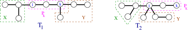
Figure 1: Example of $T_{1}\leq_{\mathsf{GTS}_{n}}T_{2}$.

The generalized tree shift operation gives us a partial order on the set of unlabelled trees with $n$ vertices, denoted by “$\leq_{\mathsf{GTS}_{n}}$”. If $T_{1}\leq_{\mathsf{GTS}_{n}}T_{2}$ and there is no tree $T$ with $T\neq T_{1},T_{2}$ such that $T_{1}\leq_{\mathsf{GTS}_{n}}T\leq_{\mathsf{GTS}_{n}}T_{2}$, then we say $T_{2}$ covers $T_{1}$ in $\mathsf{GTS}_{n}$. If either $1$ or $k$ is a leaf vertex in $T_{1}$ then it is simple to check that $T_{2}$ is isomorphic to $T_{1}$. If neither vertex $1$ nor vertex $k$ is a leaf in $T_{1}$ then $T_{2}$ covers $T_{1}$. In this case, the number of leaf vertices in $T_{2}$ is one more than the number of leaf vertices in $T_{1}$. Conversely, if $T_{2}$ covers $T_{1}$ then there exists vertices $1,k$ which witnesses the covering relation. We will use the vertices $1,k$ only for this purpose in this paper. We refer the reader to Csikvári [6] for Hasse diagram of $\mathsf{GTS}_{6}$. Csikvári [5, Theorem 2.4 and Corollary 2.5] proved the following result.

Lemma 4 (Csikvári)

Let $T$ be a tree with $n$ vertices different from $P_{n}$. Then, there exists $T^{\prime}$ such that $T^{\prime}\leq_{\mathsf{GTS}_{n}}T$. Let $T$ be a tree with $n$ vertices different from $S_{n}$. Then, there exists $T^{\prime\prime}$ such that $T\leq_{\mathsf{GTS}_{n}}T^{\prime\prime}$. Moreover, $P_{n}$ and $S_{n}$ are the only minimal and the maximal elements of $\mathsf{GTS}_{n}$ respectively.

Thus monotonicity results on $\mathsf{GTS}_{n}$ show that max-min pair is either $(P_{n},S_{n})$ or $(S_{n},P_{n})$.

2.2 $q$-Laplacian and Exponential distance matrix of a tree

For a graph $G$, let $B_{1}=\mathcal{L}_{G}^{q}|_{q=1}=L_{G}=D-A$ and $B_{2}=\mathcal{L}_{G}^{q}|_{q=-1}=D+A$, where $D$ is the diagonal matrix with degrees on the diagonal and $A$ is the adjacency matrix of $G$. It is well known that $B_{1}$ and $B_{2}$ are similar matrices for a bipartite graph $G$. Thus, when $q=\pm 1$, the $q$-Laplacian matrix $\mathcal{L}_{T}^{q}$ of a tree $T$ is positive semidefinite. In this case, all the eigenvalues of $\mathcal{L}_{T}^{q}$ are non-negative and the multiplicity of zero as an eigenvalue of $\mathcal{L}_{T}^{q}$ is $1$. Bapat, Lal and Pati [1, Propositions 3.4 and 3.7] proved the following result.

Lemma 5 (Bapat, Lal and Pati)

Let $T$ be a tree on $n$ vertices with $q$-Laplacian $\mathcal{L}_{T}^{q}$. Then,

1. $\det(\mathcal{L}_{T}^{q})=1-q^{2}$.

2. $\mathcal{L}_{T}^{q}$ is positive definite when $q\in\mathbbm{R}$ with $|q|<1$.

3. $\mathcal{L}_{T}^{q}$ has exactly one negative eigenvalue when $q\in\mathbbm{R}$ with $|q|>1$.

In [1], Bapat, Lal and Pati introduced the exponential distance matrix $\mathsf{ED}_{T}$ of a tree $T$. We recall its definition, let $T$ be a tree with $n$ vertices, then its exponential distance matrix $\mathsf{ED}_{T}=(e_{i,j})_{1\leq i,j\leq n}$ is defined as follows: the entry $e_{i,j}=1$, if $i=j$ and $e_{i,j}=q^{d_{i,j}}$, if $i\neq j$, where $d_{i,j}$ is the distance between vertex $i$ and vertex $j$ in $T$. Clearly $\mathsf{ED}_{T}$ is a symmetric matrix, hence all its eigenvalues are real. Bapat, Lal and Pati [1, Lemma 3.8] proved the following result about the relationship between the eigenvalues of $\mathcal{L}_{T}^{q}$ and $\mathsf{ED}_{T}$.

Lemma 6 (Bapat, Lal and Pati)

Let $T$ be a tree with $n$ vertices. Let $\mathcal{L}_{T}^{q}$ and $\mathsf{ED}_{T}$ be the $q$-Laplacian and the exponential distance matrix of $T$ respectively. If $q\neq\pm 1$, then $\mathsf{ED}_{T}^{-1}=\frac{1}{1-q^{2}}\mathcal{L}_{T}^{q}.$ Moreover, $\frac{1-q^{2}}{\lambda_{i}(\mathcal{L}_{T}^{q})}$ is an eigenvalue of $\mathsf{ED}_{T}$, where $\lambda_{i}(\mathcal{L}_{T}^{q})$ is an eigenvalue of $\mathcal{L}_{T}^{q}$.

Let $T$ be a tree on $n$ vertices with $q$-Laplacian $\mathcal{L}_{T}^{q}$ and exponential distance matrix $\mathsf{ED}_{T}$. Let the eigenvalues of $\mathcal{L}_{T}^{q}$ be $\lambda_{\max}(\mathcal{L}_{T}^{q})=\lambda_{1}(\mathcal{L}_{T}^{q})\geq\lambda_{2}(\mathcal{L}_{T}^{q})\geq\cdots\geq\lambda_{n}(\mathcal{L}_{T}^{q})=\lambda_{\min}(\mathcal{L}_{T}^{q})$. From Lemma 5, it is easy to see that $\lambda_{n-1}(\mathcal{L}_{T}^{q})>0$ for all $q\in\mathbbm{R}.$ Let the eigenvalues of $\mathsf{ED}_{T}$ be $\lambda_{\max}(\mathsf{ED}_{T})=\lambda_{1}(\mathsf{ED}_{T})\geq\lambda_{2}(\mathsf{ED}_{T})\geq\cdots\geq\lambda_{n}(\mathsf{ED}_{T})=\lambda_{\min}(\mathsf{ED}_{T})$. Nagar and Sivasubramanian [12, Remark 8 and Corollary 11] proved that both $\mathcal{L}_{T}^{q}|_{q=\alpha}$ and $\mathcal{L}_{T}^{q}|_{q=-\alpha}$ have the same characteristic polynomial for a tree $T$ and for all $\alpha\in\mathbbm{R}$. Thus, the multiset of eigenvalues of both the matrices $\mathcal{L}_{T}^{q}|_{q=\alpha}$ and $\mathcal{L}_{T}^{q}|_{q=-\alpha}$ are equal. This argument is used to prove the following lemma which will be used in the proof of Lemma 32.

Lemma 7

Let $T$ be a tree on $n$ vertices with $q$-Laplacian $\mathcal{L}_{T}^{q}$. Then for all $q\in\mathbbm{R}\backslash\{0\}$, the algebraic multiplicity of $\lambda_{\min}(\mathcal{L}_{T}^{q})$ as an eigenvalue of $\mathcal{L}_{T}^{q}$ is 1.

Proof:   As for all $\alpha\in\mathbbm{R}$, the multiset of eigenvalues of both the matrices $\mathcal{L}_{T}^{q}|_{q=\alpha}$ and $\mathcal{L}_{T}^{q}|_{q=-\alpha}$ are equal, it is sufficient to prove the corollary when $q\in\mathbbm{R}$ with $q>0$. We first consider the case when $q\in\mathbbm{R}$ with $q\geq 1$, from Lemma 5, $\lambda_{\min}(\mathcal{L}_{T}^{q})\leq 0$ and $\lambda_{n-1}(\mathcal{L}_{T}^{q})>0$. Thus, when $q\in\mathbbm{R}$ with $q\geq 1$, the algebraic multiplicity of $\lambda_{\min}(\mathcal{L}_{T}^{q})$ as an eigenvalue of $\mathcal{L}_{T}^{q}$ is 1.

We next consider the case when $q\in\mathbbm{R}$ with $0<q<1$. In this case each entry of the matrix $\mathsf{ED}_{T}$ is strictly positive. Therefore by Perron’s Theorem (see Horn and Johnson [9, page 526 ]), the algebraic multiplicity of $\lambda_{\max}(\mathsf{ED}_{T})$ as an eigenvalue of $\mathsf{ED}_{T}$ is $1$ for all $q\in\mathbbm{R}$ with $0<q<1$. In this case, from Lemma 6, we get the following.

$$\lambda_{\max}(\mathsf{ED}_{T})=\frac{1-q^{2}}{\lambda_{\min}(\mathcal{L}_{T}^{q})}>\frac{1-q^{2}}{\lambda_{n-1}(\mathcal{L}_{T}^{q})}=\lambda_{2}(\mathsf{ED}_{T}).$$

Thus, $\lambda_{\min}(\mathcal{L}_{T}^{q})<\lambda_{n-1}(\mathcal{L}_{T}^{q})$ for all $q\in\mathbbm{R}$ with $0<q<1$ and the proof is complete.  

Remark 8

Lemma 7 generalizes the known theorem (see Godsil and Royle [8]) that $\lambda_{2}(L_{G})>0$ for a connected graph $G$ as follows: The algebraic multiplicity of $\lambda_{\min}(L_{G})=0$ is $1$. Lemma 7 shows that for a tree $T$, the algebraic multiplicity of $\lambda_{\min}(\mathcal{L}_{T}^{q})$ for all $q\in\mathbbm{R}\backslash\{0\}$ is again $1$. It would be interesting to see if $\lambda_{2}(\mathcal{L}_{G}^{q})\neq\lambda_{1}(\mathcal{L}_{G}^{q})$ for all $q\in\mathbbm{R}\backslash\{0\}$ for all connected graphs $G$.

3 General lemma

We begin by recalling the following definition due to Csikvári [6]. Let $Q_{1}=(V_{1},E_{1})$ and $Q_{2}=(V_{2},E_{2})$ be two trees on disjoint vertex sets. Let $v_{1}\in V_{1}$ and $v_{2}\in V_{2}$. Construct a new tree $T$ by moving all the neighbours of $v_{2}$ to $v_{1}$ and then deleting $v_{2}$. We thus treat $v_{1}$ and $v_{2}$ as a single vertex in $T$. The obtained tree $T$ is denoted by $Q_{1}^{v_{1}}:Q_{2}^{v_{2}}$ and has vertex set $V(Q_{1}^{v_{1}}:Q_{2}^{v_{2}})=V_{1}\cup V_{2}-\{v_{2}\}$ and edge set $E(Q_{1}^{v_{1}}:Q_{2}^{v_{2}})=E_{1}\cup E_{2}$. We next illustrate this operation.

Let $T_{1}$ and $T_{2}$ be two trees with $n$ vertices such that $T_{2}$ covers $T_{1}$ in $\mathsf{GTS}_{n}$. Let $E(P_{k})$ be the edges on the path $P_{k}$ in $T_{1}$. Let $H_{1}$ and $H_{2}$ be the connected components of $T_{1}-E(P_{k})$ containing vertices $1$ and $k$ respectively. For the example of Figure 1, $H_{1}$ and $H_{2}$ are the subtrees of $T_{1}$ with vertex sets $X\cup\{1\}$ and $Y\cup\{k\}$ respectively. We also treat $H_{2}$ as a subtree of $T_{2}$ with vertex set $Y\cup\{1\}$. Therefore, $T_{1}=(H_{1}^{1}:P_{k}^{1})^{k}:H_{2}^{k}$ and $T_{2}=(H_{1}^{1}:P_{k}^{1})^{1}:H_{2}^{1}$. Thus, we obtain the following remark. We will use it in Section 5.

Remark 9

Let $T_{1}$ and $T_{2}$ be two trees on $n$ vertices such that $T_{2}$ covers $T_{1}$ in $\mathsf{GTS}_{n}$. Then, $|P_{k}|+|H_{1}|+|H_{2}|=n+2$. When $n$ is an even number then either all three subtrees $P_{k}$, $H_{1}$ and $H_{2}$ have an even number of vertices or exactly one subtree has an even number of vertices. Similarly, when $n$ is an odd number then either all three subtrees have an odd number of vertices or exactly one subtree has an odd number of vertices.

Let $T$ be a tree on $n$ vertices with $q$-Laplacian $\mathcal{L}_{T}^{q}$. We consider the characteristic polynomial $f^{\mathcal{L}_{T}^{q}}(q,x)=\det(xI-\mathcal{L}_{T}^{q})$. This is a bivariate polynomial. For a fixed vertex $v\in T$, let $\mathcal{L}_{T}^{q}|v$ be the submatrix obtained by deleting $v$-th row and $v$-th column from $\mathcal{L}_{T}^{q}$. Let $f^{\mathcal{L}_{T}^{q}|v}(q,x)=\det(xI-\mathcal{L}_{T}^{q}|v)$.

The following lemma is called the general lemma which was proved by Csikvári [6] for graph polynomials in one variable $x$. We will apply it to the characteristic polynomial of $\mathcal{L}_{T}^{q}$ which is a bivariate polynomial. Since the proof is identical to that of Csikvári [6, Theorem 5.1], we omit it and merely state the result.

Lemma 10

Let $Q_{1}$ and $Q_{2}$ be two trees. For any two fixed vertices $v_{1}\in Q_{1}$ and $v_{2}\in Q_{2}$, let $T=Q_{1}^{v_{1}}:Q_{2}^{v_{2}}$. Suppose

$$f^{\mathcal{L}_{T}^{q}}(q,x) = y_{1}f^{\mathcal{L}_{Q_{1}}^{q}}(q,x)f^{\mathcal{L}_{Q_{2}}^{q}}(q,x)+y_{2}f^{\mathcal{L}_{Q_{1}}^{q}}(q,x)f^{\mathcal{L}_{Q_{2}}^{q}|v_{2}}(q,x)+y_{2}f^{\mathcal{L}_{Q_{1}}^{q}|v_{1}}(q,x)f^{\mathcal{L}_{Q_{2}}^{q}}(q,x)$$ (1)

$$+y_{3}f^{\mathcal{L}_{Q_{1}}^{q}|v_{1}}(q,x)f^{\mathcal{L}_{Q_{2}}^{q}|v_{2}}(q,x),$$

where $y_{1}$, $y_{2}$, $y_{3}$ are bivariate rational functions of $q$ and $x$. Let $T_{1}$ and $T_{2}$ be two trees with $n$ vertices such that $T_{2}$ covers $T_{1}$ in $\mathsf{GTS}_{n}$ and $y_{2}f^{\mathcal{L}_{K_{2}}^{q}}(q,x)+y_{3}f^{\mathcal{L}_{K_{2}}^{q}|1}(q,x)\neq 0$, where $K_{2}$ is the complete graph on $2$ vertices. Then,

$$f^{\mathcal{L}_{T_{1}}^{q}}(q,x)-f^{\mathcal{L}_{T_{2}}^{q}}(q,x) = y_{4}\left[y_{2}f^{\mathcal{L}_{P_{k}}^{q}}(q,x)+y_{3}f^{\mathcal{L}_{P_{k}}^{q}|1}(q,x)\right]\left[y_{2}f^{\mathcal{L}_{H_{1}}^{q}}(q,x)+y_{3}f^{\mathcal{L}_{H_{1}}^{q}|1}(q,x)\right]$$

$$\times\left[y_{2}f^{\mathcal{L}_{H_{2}}^{q}}(q,x)+y_{3}f^{\mathcal{L}_{H_{2}}^{q}|1}(q,x)\right],$$

where $$y_{4}=\frac{\left[f^{\mathcal{L}_{P_{3}}^{q}|1}(q,x)-f^{\mathcal{L}_{P_{3}}^{q}|2}(q,x)\right]}{\left[y_{2}f^{\mathcal{L}_{K_{2}}^{q}}(q,x)+y_{3}f^{\mathcal{L}_{K_{2}}^{q}|1}(q,x)\right]^{2}}.$$ (2)

Let $Q_{1}$ and $Q_{2}$ be two trees and let $T=Q_{1}^{v_{1}}:Q_{2}^{v_{2}}$. Let $[m]=\{1,2,\ldots,m\}$ be the vertex set of $T$ and let $v_{1}=r=v_{2}$, where $\{1,2,\ldots,r\}$ and $\{r,r+1,\ldots,m\}$ be the vertex sets of $Q_{1}$ and $Q_{2}$ respectively. Let $\mathcal{L}_{Q_{1}}^{q}$, $\mathcal{L}_{Q_{2}}^{q}$ and $\mathcal{L}_{T}^{q}$ be the $q$-Laplacians of $Q_{1}$, $Q_{2}$ and $T$ respectively. We extend the notion of $\mathcal{L}_{T}^{q}|v$ to an arbitrary subset of $[m]$. Let $S\subseteq[m]$ and let $S^{\prime}=[m]-S$. Let $\mathcal{L}_{T}^{q}|S$ be the submatrix of $\mathcal{L}_{T}^{q}$ induced on the rows and columns with indices in the set $S^{\prime}$. We need the following lemma to obtain the rational functions $y_{1}$, $y_{2}$, $y_{3}$ and $y_{4}$.

Lemma 11

Let $\mathcal{L}_{Q_{1}}^{q}$, $\mathcal{L}_{Q_{2}}^{q}$, $\mathcal{L}_{T}^{q}$, $\mathcal{L}_{Q_{1}}^{q}|v_{1}$ and $\mathcal{L}_{Q_{2}}^{q}|v_{2}$ be the matrices as defined in the above paragraph. Let $f^{\mathcal{L}_{Q_{1}}^{q}}(q,x)$, $f^{\mathcal{L}_{Q_{2}}^{q}}(q,x)$, $f^{\mathcal{L}_{T}^{q}}(q,x)$, $f^{\mathcal{L}_{Q_{1}}^{q}|v_{1}}(q,x)$ and $f^{\mathcal{L}_{Q_{2}}^{q}|v_{2}}(q,x)$ denote the characteristic polynomials of $\mathcal{L}_{Q_{1}}^{q}$, $\mathcal{L}_{Q_{2}}^{q}$, $\mathcal{L}_{T}^{q}$, $\mathcal{L}_{Q_{1}}^{q}|v_{1}$ and $\mathcal{L}_{Q_{2}}^{q}|v_{2}$ respectively. Then, these polynomials satisfy the condition given in (1).

Proof:   Let $l_{r,r}$ denote the $(r,r)$-th entry in the bivariate polynomial matrix $xI-\mathcal{L}_{T}^{q}$. Therefore, $l_{r,r}=x-(1+q^{2}(d_{v_{1}}+d_{v_{2}}-1))$, where $d_{v_{1}}$ and $d_{v_{2}}$ are the degrees of the vertices $v_{1}$ and $v_{2}$ in $Q_{1}$ and $Q_{2}$ respectively. Let $\mu=(\mu_{i})_{1\leq i\leq r-1}$ and $\nu=(\nu_{j})_{r+1\leq j\leq m}$ be two column vectors such that $\mu_{i}=q$ if $i$ is a neighbour of $r$ in $Q_{1}$ and $\mu_{i}=0$ otherwise. Similarly, $\nu_{j}=q$ if $j$ is a neighbour of $r$ in $Q_{2}$ and $\nu_{j}=0$ otherwise. Let $R=\{1,2,\ldots,r\}$, $S=\{1,2,\ldots,r-1\}$, $R^{\prime}=[m]-R$ and $S^{\prime}=[m]-S$. Therefore,

$$xI-\mathcal{L}_{T}^{q}=\left[\begin{array}[]{c c c}N&\mu&0\\ \mu^{t}&l_{r,r}&\nu^{t}\\ 0&\nu&M\end{array}\right],\mbox{ where }M=(xI-\mathcal{L}_{T}^{q}|R)\mbox{ and }N=(xI-\mathcal{L}_{T}^{q}|S^{\prime}).$$ (3)

Clearly $\det(M)=f^{\mathcal{L}_{Q_{2}}^{q}|v_{2}}(q,x)$ and $\det(N)=f^{\mathcal{L}_{Q_{1}}^{q}|v_{1}}(q,x)$. Let $M^{\prime}=(xI-\mathcal{L}_{T}^{q}|R^{\prime})$ and $N^{\prime}=(xI-\mathcal{L}_{T}^{q}|S)$. Then, it is simple to see the following.

$$\det(M^{\prime}) = \det\left[\begin{array}[]{ c c}N&\mu\\ \mu^{t}&x-(1+q^{2}(d_{v_{1}}+d_{v_{2}}-1))\end{array}\right]=f^{\mathcal{L}_{Q_{1}}^{q}}(q,x)-q^{2}d_{v_{2}}f^{\mathcal{L}_{Q_{1}}^{q}|v_{1}}(q,x).$$ (6)

$$\det(N^{\prime}) = \det\left[\begin{array}[]{ c c}x-(1+q^{2}(d_{v_{1}}+d_{v_{2}}-1))&\nu^{t}\\ \nu&M\end{array}\right]=f^{\mathcal{L}_{Q_{2}}^{q}}(q,x)-q^{2}d_{v_{1}}f^{\mathcal{L}_{Q_{2}}^{q}|v_{2}}(q,x).$$ (9)

From (3), when we expand $\det(xI-\mathcal{L}_{T}^{q})$ with respect to the $r$-th row, we get

$$f^{\mathcal{L}_{T}^{q}}(q,x) = \det(xI-\mathcal{L}_{T}^{q})=\det(M^{\prime})\det(M)+\det(N)\det(N^{\prime})-l_{r,r}\det(N)\det(M)$$ (10)

$$= \left[f^{\mathcal{L}_{Q_{1}}^{q}}(q,x)-q^{2}d_{v_{2}}f^{\mathcal{L}_{Q_{1}}^{q}|v_{1}}(q,x)\right]f^{\mathcal{L}_{Q_{2}}^{q}|v_{2}}(q,x)$$

$$+f^{\mathcal{L}_{Q_{1}}^{q}|v_{1}}(q,x)\left[f^{\mathcal{L}_{Q_{2}}^{q}}(q,x)-q^{2}d_{v_{1}}f^{\mathcal{L}_{Q_{2}}^{q}|v_{2}}(q,x)\right]$$

$$-\left(x-(1+q^{2}(d_{v_{1}}+d_{v_{2}}-1))\right)f^{\mathcal{L}_{Q_{1}}^{q}|v_{1}}(q,x)f^{\mathcal{L}_{Q_{2}}^{q}|v_{2}}(q,x)$$

$$= f^{\mathcal{L}_{Q_{1}}^{q}}(q,x)f^{\mathcal{L}_{Q_{2}}^{q}|v_{2}}(q,x)+f^{\mathcal{L}_{Q_{2}}^{q}}(q,x)f^{\mathcal{L}_{Q_{1}}^{q}|v_{1}}(q,x)$$

$$-(x-1+q^{2})f^{\mathcal{L}_{Q_{1}}^{q}|v_{1}}(q,x)f^{\mathcal{L}_{Q_{2}}^{q}|v_{2}}(q,x),$$

where the third equality follows from (6) and (9). The last equality follows by doing simple manipulations completing the proof.  

Let $T$ be a tree with $q$-Laplacian $\mathcal{L}_{T}^{q}$. For a fixed $q\in\mathbbm{R}\backslash\{0\}$ and for a fixed vertex $v\in T$, define the auxiliary polynomial

$$\mathcal{F}_{T}^{v}(q,x)=f^{\mathcal{L}_{T}^{q}}(q,x)-(x+q^{2}-1)f^{\mathcal{L}_{T}^{q}|v}(q,x).$$ (11)

We recall that $P_{k}$, $H_{1}$ and $H_{2}$ are the subtrees of $T_{1}$ and $T_{2}$, where $T_{2}$ covers $T_{1}$ in $\mathsf{GTS}_{n}$. From (1) and (10), we get the rational functions $y_{1}=0$, $y_{2}=1$, $y_{3}=-(x-1+q^{2})$.

Theorem 12

Let $T_{1}$ and $T_{2}$ be two trees on $n$ vertices with $q$-Laplacians $\mathcal{L}_{T_{1}}^{q}$ and $\mathcal{L}_{T_{2}}^{q}$ respectively. Let $T_{2}$ cover $T_{1}$ in $\mathsf{GTS}_{n}$. Then, for all $q\in\mathbbm{R}\backslash\{0\}$

$$f^{\mathcal{L}_{T_{1}}^{q}}(q,x)-f^{\mathcal{L}_{T_{2}}^{q}}(q,x)=-\frac{1}{q^{2}x}\mathcal{F}_{P_{k}}^{1}(q,x)\mathcal{F}_{H_{1}}^{1}(q,x)\mathcal{F}_{H_{2}}^{1}(q,x),$$

where $\mathcal{F}_{P_{k}}^{1}(q,x)$, $\mathcal{F}_{H_{1}}^{1}(q,x)$ and $\mathcal{F}_{H_{2}}^{1}(q,x)$ are the polynomials defined in (11).

Proof:   From Lemma 11, we get $y_{1}=0$, $y_{2}=1$, $y_{3}=-(x-1+q^{2})$. Therefore when $q\in\mathbbm{R}\backslash\{0\}$

$$y_{2}f^{\mathcal{L}_{K_{2}}^{q}}(q,x)+y_{3}f^{\mathcal{L}_{K_{2}}^{q}|1}(q,x)=(x-1)^{2}-q^{2}-(x-1+q^{2})(x-1)=-q^{2}x\neq 0.$$

Note that $f^{\mathcal{L}_{P_{3}}^{q}|1}(q,x)-f^{\mathcal{L}_{P_{3}}^{q}|2}(q,x)=-q^{2}x.$ Thus, by (2), we have $\displaystyle y_{4}=-1/q^{2}x$. Using Lemma 10, the proof is complete.  

4 Interlacing of eigenvalues of $\mathcal{L}_{T}^{q}$

Let $A$ be an $n\times n$ real symmetric matrix. We order the eigenvalues of $A$ as $\lambda_{1}(A)\geq\lambda_{2}(A)\geq\cdots\geq\lambda_{n}(A).$ We need the following lemma from Molitierno [11, Theorem 1.2.8 and Corollary 1.2.11].

Lemma 13

Let $A,B$ be two $n\times n$ real symmetric matrices with $B=zz^{t}$ for some column vector $z\in\mathbbm{R}^{n}$. Then,

$$\lambda_{1}(A+B)\geq\lambda_{1}(A)\geq\cdots\geq\lambda_{n}(A+B)\geq\lambda_{n}(A).$$

We have two interlacing lemmas about the eigenvalues of $\mathcal{L}_{T}^{q}$ when $q\in\mathbbm{R}$ with either $|q|\leq 1$ or $|q|>1$. The following result is an interlacing lemma about the eigenvalues of $\mathcal{L}_{T}^{q}$ when $|q|\leq 1$.

Lemma 14

Let $T$ be a tree on $n$ vertices with a leaf vertex $l$. Let $T^{\prime}=T-\{l\}$. Let $\mathcal{L}_{T}^{q}$ and $\mathcal{L}_{T^{\prime}}^{q}$ be the $q$-Laplacians of $T$ and $T^{\prime}$ respectively. Then, for $q\in\mathbbm{R}$ with $|q|\leq 1$,

$$\lambda_{1}(\mathcal{L}_{T}^{q})\geq\lambda_{1}(\mathcal{L}_{T^{\prime}}^{q})\geq\cdots\geq\lambda_{n-1}(\mathcal{L}_{T^{\prime}}^{q})\geq\lambda_{n}(\mathcal{L}_{T}^{q})\geq 0.$$

Proof:   We can without loss of generality assume in $T$ that $l=n$ is the deleted leaf vertex with neighbour $n-1$. Let $e_{n-1}=[0,0,\ldots,0,1]^{t}\in\mathbbm{R}^{n-1}$. Then,

$$\mathcal{L}_{T}^{q} = \left[\begin{array}[]{c c}q^{2}e_{n-1}e^{t}_{n-1}+\mathcal{L}_{T^{\prime}}^{q}&-qe_{n-1}\\ -qe^{t}_{n-1}&1\end{array}\right]=\left[\begin{array}[]{c c}\mathcal{L}_{T^{\prime}}^{q}&0\\ 0&0\end{array}\right]+\left[\begin{array}[]{c c}q^{2}e_{n-1}e^{t}_{n-1}&-qe_{n-1}\\ -qe^{t}_{n-1}&1\end{array}\right]$$

$$= \left[\begin{array}[]{c c}\mathcal{L}_{T^{\prime}}^{q}&0\\ 0&0\end{array}\right]+zz^{t},\mbox{ where }z=[0,0,\ldots,0,-q,1]^{t}\in\mathbbm{R}^{n}.$$

By Lemma 5, both $\mathcal{L}_{T}^{q}$ and $\mathcal{L}_{T^{\prime}}^{q}$ are positive semidefinite when $|q|\leq 1$. Therefore, all the eigenvalues of $\mathcal{L}_{T}^{q}$ and $\mathcal{L}_{T^{\prime}}^{q}$ are non-negative. Thus, by using Lemma 13, we have $\lambda_{1}(\mathcal{L}_{T}^{q})\geq\lambda_{1}(\mathcal{L}_{T^{\prime}}^{q})\geq\cdots\geq\lambda_{n-1}(\mathcal{L}_{T^{\prime}}^{q})\geq\lambda_{n}(\mathcal{L}_{T}^{q})\geq 0$ completing the proof.  

From Lemma 5, $\mathcal{L}_{T}^{q}$ is not positive semidefinite when $q\in\mathbbm{R}$ with $|q|>1$. We prove the following partial interlacing lemma about the eigenvalues of $\mathcal{L}_{T}^{q}$ when $|q|>1$.

Lemma 15

Let $T$ be a tree on $n$ vertices with a leaf vertex $l$. Let $T^{\prime}=T-\{l\}$. Let $\mathcal{L}_{T}^{q}$ and $\mathcal{L}_{T^{\prime}}^{q}$ be the $q$-Laplacians of $T$ and $T^{\prime}$ respectively. Then, for $q\in\mathbbm{R}$ with $|q|>1$,

$$\lambda_{1}(\mathcal{L}_{T}^{q})\geq\lambda_{1}(\mathcal{L}_{T^{\prime}}^{q})\geq\cdots\geq\lambda_{n-2}(\mathcal{L}_{T^{\prime}}^{q})\geq\lambda_{n-1}(\mathcal{L}_{T}^{q})>0>\lambda_{n}(\mathcal{L}_{T}^{q})\geq\lambda_{n-1}(\mathcal{L}_{T^{\prime}}^{q}).$$

Proof:   As done in Lemma 14, we assume the vertex $l=n$ and that its neighbour is vertex $n-1$. Thus, we obtain $\mathcal{L}_{T}^{q}=A+B$, where

$$A=\left[\begin{array}[]{c c}\mathcal{L}_{T^{\prime}}^{q}&0\\ 0&0\end{array}\right]\mbox{ and }B=zz^{t}\mbox{ with }z=[0,0,\ldots,0,-q,1]^{t}\in\mathbbm{R}^{n}.$$

By Lemma 5, both $\mathcal{L}_{T}^{q}$ and $\mathcal{L}_{T^{\prime}}^{q}$ have exactly one negative eigenvalue and both $\mathcal{L}_{T}^{q}$ and $\mathcal{L}_{T^{\prime}}^{q}$ are invertible when $|q|>1$. Therefore, the eigenvalues of $A$ are the following: $\lambda_{1}(\mathcal{L}_{T^{\prime}}^{q})\geq\cdots\geq\lambda_{n-2}(\mathcal{L}_{T^{\prime}}^{q})>0>\lambda_{n-1}(\mathcal{L}_{T^{\prime}}^{q}).$ Thus, by Lemma 13, $\lambda_{1}(\mathcal{L}_{T}^{q})\geq\lambda_{1}(\mathcal{L}_{T^{\prime}}^{q})\geq\cdots\geq\lambda_{n-1}(\mathcal{L}_{T}^{q})>0>\lambda_{n}(\mathcal{L}_{T}^{q})\geq\lambda_{n-1}(\mathcal{L}_{T^{\prime}}^{q})$ completing the proof.  

Let $T$ be a tree on $n$ vertices with $q$-Laplacian $\mathcal{L}_{T}^{q}$. Let $\lambda_{\max}(\mathcal{L}_{T}^{q})$, $\lambda_{\min}(\mathcal{L}_{T}^{q})$ and $\lambda_{a}(\mathcal{L}_{T}^{q})=\lambda_{n-1}(\mathcal{L}_{T}^{q})$ denote the largest, the smallest and the second smallest eigenvalues of $\mathcal{L}_{T}^{q}$ respectively. We need the following corollaries of Lemmas 14 and 15.

Corollary 16

Let $T$ be a tree with $n$ vertices and let $T^{\prime}$ be a subtree of $T$. Let $\mathcal{L}_{T}^{q}$ and $\mathcal{L}_{T^{\prime}}^{q}$ be the $q$-Laplacians of $T$ and $T^{\prime}$ respectively. Then, for all $q\in\mathbbm{R}$, $\lambda_{\max}(\mathcal{L}_{T^{\prime}}^{q})\leq\lambda_{\max}(\mathcal{L}_{T}^{q}).$

Proof:   Let $T^{\prime}=T_{0}$ be the given subtree of $T$ and let $m$ be the number of vertices in $T_{0}$. Construct a new tree $T_{1}$ by adding a leaf vertex in $T_{0}$ such that $T_{1}$ is again a subtree of $T$. Thus, from Lemmas 14 and 15, $\lambda_{\max}(\mathcal{L}_{T_{0}}^{q})\leq\lambda_{\max}(\mathcal{L}_{T_{1}}^{q})$ for all $q\in\mathbbm{R}$. By repeating this process we get a sequence of subtrees $T^{\prime}=T_{0}$, $T_{1}$, $\ldots$, $T_{n-m}=T$ of $T$ with $\lambda_{\max}(\mathcal{L}_{T^{\prime}}^{q})=\lambda_{\max}(\mathcal{L}_{T_{0}}^{q})\leq\lambda_{\max}(\mathcal{L}_{T_{1}}^{q})\leq\cdots\leq\lambda_{\max}(\mathcal{L}_{T_{n-m}}^{q})=\lambda_{\max}(\mathcal{L}_{T}^{q})$ and hence, completing the proof.  

By using similar argument as done in the proof of Corollary 16, we see that $\lambda_{a}(\mathcal{L}_{T^{\prime}}^{q})\geq\lambda_{a}(\mathcal{L}_{T}^{q})$, where $T^{\prime}$ is a subtree of $T$. Thus, we obtain the following corollary of Lemmas 14 and 15.

Corollary 17

Using the notations of Theorem 12, let $P_{k}$, $H_{1}$ and $H_{2}$ be the subtrees of both $T_{1}$ and $T_{2}$. Then, for all $q\in\mathbbm{R}$, we have $\max\left(\lambda_{a}(\mathcal{L}_{T_{1}}^{q}),\lambda_{a}(\mathcal{L}_{T_{2}}^{q})\right)\leq\min\left(\lambda_{a}(\mathcal{L}_{P_{k}}^{q}),\lambda_{a}(\mathcal{L}_{H_{1}}^{q}),\lambda_{a}(\mathcal{L}_{H_{2}}^{q})\right).$

5 Auxiliary polynomial $\mathcal{F}_{T}^{v}(q,x)$

Let $T$ be a tree on $n$ vertices with $q$-Laplacian $\mathcal{L}_{T}^{q}$. We recall the definition of the polynomial $\mathcal{F}_{T}^{v}(q,x)$ defined in (11) as follows:

$$\mathcal{F}_{T}^{v}(q,x)=f^{\mathcal{L}_{T}^{q}}(q,x)-(x-1+q^{2})f^{\mathcal{L}_{T}^{q}|v}(q,x)=f^{\mathcal{L}_{T}^{q}}(q,x)-(x-\det(\mathcal{L}_{T}^{q}))f^{\mathcal{L}_{T}^{q}|v}(q,x).$$

We think of $\mathcal{F}_{T}^{v}(q,x)$ as a univariate polynomial once a real value for $q$ is assigned. From Theorem 12, we recall that when a tree $T_{2}$ covers an another tree $T_{1}$ in $\mathsf{GTS}_{n}$, $f^{\mathcal{L}_{T_{1}}^{q}}(q,x)-f^{\mathcal{L}_{T_{2}}^{q}}(q,x)$ is a product of three auxiliary polynomials of subtrees $P_{k}$, $H_{1}$, and $H_{2}$ of $T_{1}$ and $T_{2}$. Therefore the roots of this difference polynomial is the multiset union of the roots of auxiliary polynomials of these subtrees $P_{k}$, $H_{1}$, and $H_{2}$. Thus, to prove Theorem 2, we need to determine the location of all these roots and decide the sign of $f^{\mathcal{L}_{T_{1}}^{q}}(q,x)-f^{\mathcal{L}_{T_{2}}^{q}}(q,x)$ for a fixed $q\in\mathbbm{R}\backslash\{0\}$ and when $x\in[(-\infty,t_{1})\cup(t_{2},\infty)]-\{0\}$, where $t_{1}=\max(\lambda_{a}(\mathcal{L}_{T_{1}}^{q}),\lambda_{a}(\mathcal{L}_{T_{2}}^{q}))$ and $t_{2}=\min(\lambda_{\max}(\mathcal{L}_{T_{1}}^{q}),\lambda_{\max}(\mathcal{L}_{T_{2}}^{q}))$.

Lemma 18

For a tree $T$ on $n>1$ vertices with $q$-Laplacian $\mathcal{L}_{T}^{q}$, the degree of $\mathcal{F}_{T}^{v}(q,x)$ is $n-1$ and the coefficient of $x^{n-1}$ in $\mathcal{F}_{T}^{v}(q,x)$ is $-q^{2}d_{v}$. Further, for all $q\in\mathbbm{R}\backslash\{0\}$, zero is a root of $\mathcal{F}_{T}^{v}(q,x)$.

Proof:   Without loss of generality we assume that the first row of $\mathcal{L}_{T}^{q}$ is indexed by the vertex $v$. Let $\alpha=(\alpha_{i})_{2\leq i\leq n}$ be a column vector such that $\alpha_{i}=q$ if $v$ is adjacent to the vertex $i$ and $\alpha_{i}=0$ otherwise. Therefore

$$f^{\mathcal{L}_{T}^{q}}(q,x) = \det\left[\begin{array}[]{c c}x-1-q^{2}(d_{v}-1)&\alpha^{t}\\ \alpha&xI-\mathcal{L}_{T}^{q}|v\end{array}\right]$$ (16)

$$= \det\left[\begin{array}[]{c c}x-1+q^{2}&\alpha^{t}\\ 0&xI-\mathcal{L}_{T}^{q}|v\end{array}\right]+\det\left[\begin{array}[]{c c}-q^{2}d_{v}&\alpha^{t}\\ \alpha&xI-\mathcal{L}_{T}^{q}|v\end{array}\right]$$ (21)

$$= (x-1+q^{2})f^{\mathcal{L}_{T}^{q}|v}(q,x)+\det\left[\begin{array}[]{c c}-q^{2}d_{v}&\alpha^{t}\\ \alpha&xI-\mathcal{L}_{T}^{q}|v\end{array}\right]$$ (24)

From the definition of $\mathcal{F}_{T}^{v}(q,x)$ and by using (24), it is easy to see that the degree of the polynomial $\mathcal{F}_{T}^{v}(q,x)$ in the variable $x$ is $n-1$ and the coefficient of $x^{n-1}$ in $\mathcal{F}_{T}^{v}(q,x)$ is $-q^{2}d_{v}$.

Nagar and Sivasubramanian [12, Remark 13] proved that $f^{\mathcal{L}_{T}^{q}|v}(q,0)=(-1)^{n-1}$. Thus, when $x=0$ from Lemma 5, we get the following.

$$\mathcal{F}_{T}^{v}(q,0)=f^{\mathcal{L}_{T}^{q}}(q,0)-(q^{2}-1)f^{\mathcal{L}_{T}^{q}|v}(q,0)=(-1)^{n}\det(\mathcal{L}_{T}^{q})-(q^{2}-1)(-1)^{n-1}=0.$$

Thus, zero is a root of $\mathcal{F}_{T}^{v}(q,x)$ and hence the proof is complete.  

For a fixed $q\in\mathbbm{R}\backslash\{0\}$, from Lemma 18, it is easy to see that for large positive $x$ the function $\mathcal{F}_{T}^{v}(q,x)$ is negative. When $|q|\leq 1$, we next prove that the multiplicity of zero as a root of $\mathcal{F}_{T}^{v}(q,x)$ is one and determine the location of its $n-2$ non-zero roots. Let the eigenvalues of $\mathcal{L}_{T}^{q}|v$ be $\lambda_{1}(\mathcal{L}_{T}^{q}|v)\geq\lambda_{2}(\mathcal{L}_{T}^{q}|v)\geq\cdots\geq\lambda_{n-1}(\mathcal{L}_{T}^{q}|v)$. Let $\sigma(\mathcal{L}_{T}^{q}|v)=\{\lambda_{1}(\mathcal{L}_{T}^{q}|v),\ldots,\lambda_{n-1}(\mathcal{L}_{T}^{q}|v)\}$ be the multiset of eigenvalues of $\mathcal{L}_{T}^{q}|v$. From [12, Corollary 12], it is simple to see that all the eigenvalues of $\mathcal{L}_{T}^{q}|v$ are non-negative. Let $\sigma(\mathcal{L}_{T}^{q})=\{\lambda_{1}(\mathcal{L}_{T}^{q}),\ldots,\lambda_{n-1}(\mathcal{L}_{T}^{q})\}$ be the multisets of the $n-1$ largest eigenvalues of $\mathcal{L}_{T}^{q}$. Motivated by Csikvári [6, the third part of Theorem 7.3] when $q\in\mathbbm{R}$ with $|q|\leq 1$, we obtain the following result.

Lemma 19

Let $T$ be a tree on $n>1$ vertices and let $v\in T$. Then, for a fixed $q\in\mathbbm{R}\backslash\{0\}$ with $|q|\leq 1$, each non-zero root of $\mathcal{F}_{T}^{v}(q,x)$ lies in the interval $[\lambda_{a}(\mathcal{L}_{T}^{q}),\lambda_{\max}(\mathcal{L}_{T}^{q})]$.

Proof:   Using the Interlacing Theorem for eigenvalues of symmetric matrices (see Godsil and Royle [8, page 193]), we get the following.

$$\lambda_{1}(\mathcal{L}_{T}^{q})\geq\lambda_{1}(\mathcal{L}_{T}^{q}|v)\geq\cdots\geq\lambda_{i}(\mathcal{L}_{T}^{q})\geq\lambda_{i}(\mathcal{L}_{T}^{q}|v)\geq\cdots\geq\lambda_{n-1}(\mathcal{L}_{T}^{q}|v)\geq\lambda_{n}(\mathcal{L}_{T}^{q}).$$ (25)

We break the proof into two cases when $1-q^{2}\geq\lambda_{n-1}(\mathcal{L}_{T}^{q})$ and when $1-q^{2}<\lambda_{n-1}(\mathcal{L}_{T}^{q}).$ For both the cases, the proof is identical. Thus, we only consider the case when $1-q^{2}\geq\lambda_{n-1}(\mathcal{L}_{T}^{q})$.

Firstly we assume that $\sigma(\mathcal{L}_{T}^{q})\Cap\left[\sigma(\mathcal{L}_{T}^{q}|v)\Cup\{1-q^{2}\}\right]=\emptyset$, where $\Cap$ and $\Cup$ denote the multiset intersection and multiset union respectively. Therefore from (25), the multiplicity of each eigenvalue of $\mathcal{L}_{T}^{q}$ and $\mathcal{L}_{T}^{q}|v$ is one and we get

$$\lambda_{1}(\mathcal{L}_{T}^{q})>\lambda_{1}(\mathcal{L}_{T}^{q}|v)>\cdots>\lambda_{n-1}(\mathcal{L}_{T}^{q})>\lambda_{n-1}(\mathcal{L}_{T}^{q}|v)\mbox{ with }1-q^{2}>\lambda_{n-1}(\mathcal{L}_{T}^{q}).$$ (26)

It is easy to see that

$$\lambda_{\max}(\mathcal{L}_{T}^{q}) \geq \frac{\sum_{i=0}^{n}\lambda_{i}(\mathcal{L}_{T}^{q})}{n}=\frac{\mathsf{Trace}(\mathcal{L}_{T}^{q})}{n}=\frac{\sum_{v\in T}1+q^{2}(d_{v}-1)}{n}=\frac{n+q^{2}(n-2)}{n}$$ (27)

$$\geq 1-q^{2}.$$

Thus, from (26) and (27), $1-q^{2}$ is sandwiched between two eigenvalues of $\mathcal{L}_{T}^{q}$. Thus, for some $i$ with $1\leq i\leq n-2$, we get

$$\lambda_{i}(\mathcal{L}_{T}^{q})>\lambda_{i}(\mathcal{L}_{T}^{q}|v)>\lambda_{i+1}(\mathcal{L}_{T}^{q})\mbox{ with }\lambda_{i}(\mathcal{L}_{T}^{q})>m_{1}\geq m_{2}>\lambda_{i+1}(\mathcal{L}_{T}^{q}),$$

where $m_{1}=\max\left(1-q^{2},\lambda_{i}(\mathcal{L}_{T}^{q}|v)\right)$ and $m_{2}=\min\left(1-q^{2},\lambda_{i}(\mathcal{L}_{T}^{q}|v)\right)$. Recall for a fixed $q\in\mathbbm{R}\backslash\{0\}$, the polynomial $\mathcal{F}_{T}^{v}(q,x)$ is univariate in the variable $x$. Thus, by the intermediate value theorem (IVT henceforth), as both the quantities $\mathcal{F}_{T}^{v}(q,m_{1})=f^{\mathcal{L}_{T}^{q}}(q,m_{1})$ and $\mathcal{F}_{T}^{v}(q,m_{2})=f^{\mathcal{L}_{T}^{q}}(q,m_{2})$ have same sign, either both are positive or both are negative.

From Lemma 18, we recall that for large positive $x\in\mathbbm{R}$, $\mathcal{F}_{T}^{v}(q,x)$ is negative. When $1<i$, $\lambda_{1}(\mathcal{L}_{T}^{q})>\lambda_{1}(\mathcal{L}_{T}^{q}|v)>m_{1}$ and the coefficient of $x^{n-1}$ in $f^{\mathcal{L}_{T}^{q}|v}(q,x)$ is positive. Therefore $\mathcal{F}_{T}^{v}(q,\lambda_{1}(\mathcal{L}_{T}^{q}))=-(\lambda_{1}(\mathcal{L}_{T}^{q})-1+q^{2})f^{\mathcal{L}_{T}^{q}|v}(q,\lambda_{1}(\mathcal{L}_{T}^{q}))$ is negative. Similarly when $2<i$, the coefficient of $x^{n}$ in $f^{\mathcal{L}_{T}^{q}}(q,x)$ is positive and $\lambda_{1}(\mathcal{L}_{T}^{q})>\lambda_{1}(\mathcal{L}_{T}^{q}|v)>\lambda_{2}(\mathcal{L}_{T}^{q})>m_{1}$. Thus, by the IVT, $\mathcal{F}_{T}^{v}(q,\lambda_{1}(\mathcal{L}_{T}^{q}|v))=f^{\mathcal{L}_{T}^{q}}(q,\lambda_{1}(\mathcal{L}_{T}^{q}|v))$ is again negative. By using identical arguments when $x\in\{\lambda_{2}(\mathcal{L}_{T}^{q}),\lambda_{2}(\mathcal{L}_{T}^{q}|v)\}$ with $\lambda_{2}(\mathcal{L}_{T}^{q}|v)>m_{1}$, $\mathcal{F}_{T}^{v}(q,x)$ is positive. $\mathcal{F}_{T}^{v}(q,x)$ is negative if $j$ is odd and positive if $j$ is even. But when $j=i$, both the quantities $\mathcal{F}_{T}^{v}(q,m_{1})$ and $\mathcal{F}_{T}^{v}(q,m_{2})$ have the same sign. Therefore, it is easy to extend this for all $j$ with $1\leq j\leq n-1$. Thus, when $x\in\left\{\lambda_{j}(\mathcal{L}_{T}^{q}),\lambda_{j}(\mathcal{L}_{T}^{q}|v)\right\}$ $\mathcal{F}_{T}^{v}(q,x)$ is negative if $j$ is odd and positive if $j$ is even. Hence, there must be a root of $\mathcal{F}_{T}^{v}(q,x)$ in the interval $[\lambda_{j+1}(\mathcal{L}_{T}^{q}),\lambda_{j}(\mathcal{L}_{T}^{q}|v)]$ for $j=1,2,\ldots,n-2$. See Example 21 for better interpretation.

Secondly we assume that $\sigma(\mathcal{L}_{T}^{q})\Cap\left[\sigma(\mathcal{L}_{T}^{q}|v)\Cup\{1-q^{2}\}\right]=\{\lambda_{1},\lambda_{2},\ldots,\lambda_{c}\}$. Clearly $\lambda_{1}$, $\lambda_{2}$, $\ldots$, $\lambda_{c}$ are the roots of $\mathcal{F}_{T}^{v}(q,x)$ and these lie in the interval $[\lambda_{a}(\mathcal{L}_{T}^{q}),\lambda_{\max}(\mathcal{L}_{T}^{q})]$. From (25), it is clear that the multiplicity of each eigenvalue not containing in $\{\lambda_{1},\ldots,\lambda_{c}\}$ of $\mathcal{L}_{T}^{q}$ and $\mathcal{L}_{T}^{q}|v$ is one. Therefore the remaining eigenvalues of $\mathcal{L}_{T}^{q}$ and $\mathcal{L}_{T}^{q}|v$ satisfy an identical relation as given in (26). Thus, by using similar arguments as done in the above paragraph, it is easy to determine the location of the remaining $n-c-2$ roots of $\mathcal{F}_{T}^{v}(q,x)$ by locating the roots of the following polynomial.

$$\frac{\mathcal{F}_{T}^{v}(q,x)}{\prod_{i=1}^{c}(x-\lambda_{i})}=\frac{f^{\mathcal{L}_{T}^{q}}(q,x)}{\prod_{i=1}^{c}(x-\lambda_{i})}-\frac{(x-1+q^{2})f^{\mathcal{L}_{T}^{q}|v}(q,x)}{\prod_{i=1}^{c}(x-\lambda_{i})}.$$

Thus, for $q\in\mathbbm{R}\backslash\{0\}$ with $|q|\leq 1$, all the non-zero roots of $\mathcal{F}_{T}^{v}(q,x)$ lie in the interval $[\lambda_{a}(\mathcal{L}_{T}^{q}),\lambda_{\max}(\mathcal{L}_{T}^{q})]$. The proof is complete.  

When $q\in\mathbbm{R}$ with $|q|>1$, the proof of the following lemma is identical to the proof of Lemma 19.

Lemma 20

Let $T$ be a tree on $n>1$ vertices and let $v\in T$. Then, for all $q\in\mathbbm{R}$ with $|q|>1$, each non-zero roots of $\mathcal{F}_{T}^{v}(q,x)$ lies in the interval $[\lambda_{a}(\mathcal{L}_{T}^{q}),\lambda_{\max}(\mathcal{L}_{T}^{q})]$.

Proof:   For a fixed $q\in\mathbbm{R}$ with $|q|>1$ from Lemma 5, $\lambda_{n}(\mathcal{L}_{T}^{q})<0$, $\lambda_{n-1}(\mathcal{L}_{T}^{q})>0$ and $\det(\mathcal{L}_{T}^{q})=1-q^{2}<0$. We recall that $\lambda_{n-1}(\mathcal{L}_{T}^{q}|v)\geq 0$. Therefore, the interlacing theorem for eigenvalues of symmetric matrices gives the following.

$$\lambda_{1}(\mathcal{L}_{T}^{q})\geq\lambda_{1}(\mathcal{L}_{T}^{q}|v)\geq\cdots\geq\lambda_{n-1}(\mathcal{L}_{T}^{q}|v)>\max\left(1-q^{2},\lambda_{n}(\mathcal{L}_{T}^{q})\right)\ geq\min\left(1-q^{2},\lambda_{n}(\mathcal{L}_{T}^{q})\right).$$

By using identical arguments as done in the proof of Lemma 19, all the non-zero roots of $\mathcal{F}_{T}^{v}(q,x)$ lie in the interval $[\lambda_{a}(\mathcal{L}_{T}^{q}),\lambda_{\max}(\mathcal{L}_{T}^{q}|v)]$ for all $q\in\mathbbm{R}$ with $|q|>1$. The proof is complete.  

The following example illustrates Lemmas 19 and 20.

Example 21

Let $T_{1}$ be the tree given in Figure 4. For all $x\in[\lambda_{\min}(\mathcal{L}_{T_{1}}^{q}),\lambda_{\max}(\mathcal{L}_{T_{1}}^{q})]$ with $q=0.5$ and $q=1.5$ some values of $f^{\mathcal{L}_{T_{1}}^{q}}(q,x)$, $f^{\mathcal{L}_{T_{1}}^{q}|1}(q,x)$ and $\mathcal{F}_{T_{1}}^{1}(q,x)$ are drawn in Figures 3 and 3 respectively. $1$ is an eigenvalue of both the matrices $\mathcal{L}_{T_{1}}^{q}$ and $\mathcal{L}_{T_{1}}^{q}|1$. Thus, $1$ is a root of $\mathcal{F}_{T_{1}}^{1}(q,x)$. Here, the solid red, dotted blue and thick solid black lines are used for $f^{\mathcal{L}_{T_{1}}^{q}}(q,x)$, $f^{\mathcal{L}_{T_{1}}^{q}|1}(q,x)$ and $\mathcal{F}_{T}^{1}(q,x)$ respectively. Arrows on lines are used for the behaviour of these polynomials when $x$ decreases from $\lambda_{\max}(\mathcal{L}_{T_{1}}^{q})$ to $\lambda_{\min}(\mathcal{L}_{T_{1}}^{q}).$ These polynomials were drawn by using the computer package SageMath.

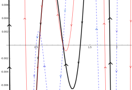
Figure 2: The values of $f^{\mathcal{L}_{T_{1}}^{q}}(0.5,x)$, $f^{\mathcal{L}_{T_{1}}^{q}|1}(0.5,x)$ and $\mathcal{F}_{T_{1}}^{1}(0.5,x)$.

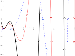
Figure 3: The values of $f^{\mathcal{L}_{T_{1}}^{q}}(1.5,x)$, $f^{\mathcal{L}_{T_{1}}^{q}|1}(1.5,x)$ and $\mathcal{F}_{T_{1}}^{1}(1.5,x)$.

We recall that zero is a root of $\mathcal{F}_{T}^{v}(q,x)$ with multiplicity one and the second smallest root of $\mathcal{F}_{T}^{v}(q,x)$ lies in the interval $[\lambda_{a}(\mathcal{L}_{T}^{q}),\lambda_{n-2}(\mathcal{L}_{T}^{q}|v)]$, where $\lambda_{a}(\mathcal{L}_{T}^{q})>0$ and $\lambda_{n-2}(\mathcal{L}_{T}^{q}|v)>0$ are the second smallest eigenvalues of $\mathcal{L}_{T}^{q}$ and $\mathcal{L}_{T}^{q}|v$ respectively. Thus, by Lemmas 18, 19 and 20, we obtain the following.

Remark 22

Let $T$ be a tree on $n$ vertices and let $v\in T$. Then, for a fixed $q\in\mathbbm{R}\backslash\{0\}$ and for $x\in(-\infty,0)$ the polynomial $\mathcal{F}_{T}^{v}(q,x)$ is positive when $n$ is even and negative when $n$ is odd. Moreover, by the IVT, for all $x\in(0,\lambda_{a}(\mathcal{L}_{T}^{q}))$, we have $\mathcal{F}_{T}^{v}(q,x)<0$ when $n$ is even and $\mathcal{F}_{T}^{v}(q,x)>0$ when $n$ is odd.

Let $T_{1}$ and $T_{2}$ be two trees with $n$ vertices such that $T_{2}$ covers $T_{1}$ in $\mathsf{GTS}_{n}$. For convenience, from Theorem 12, we define

$$\mathcal{D}_{T_{2}}^{T_{1}}(q,x)=f^{\mathcal{L}_{T_{1}}^{q}}(q,x)-f^{\mathcal{L}_{T_{2}}^{q}}(q,x)=-\frac{1}{q^{2}x}\mathcal{F}_{P_{k}}^{1}(q,x)\mathcal{F}_{H_{1}}^{1}(q,x)\mathcal{F}_{H_{2}}^{1}(q,x),\mbox{ \rm{ where } }q\neq 0.$$ (28)

From Lemma 18, zero is a root of all the three polynomials $\mathcal{F}_{P_{k}}^{1}(q,x)$, $\mathcal{F}_{H_{1}}^{1}(q,x)$ and $\mathcal{F}_{H_{2}}^{1}(q,x)$ with multiplicity one. Thus, from (28), zero is a root of $\mathcal{D}_{T_{2}}^{T_{1}}(q,x)$ with multiplicity two. We need the following lemma in Section 6.

Lemma 23

Let $T_{1}$ and $T_{2}$ be two trees with $n$ vertices such that $T_{2}$ covers $T_{1}$ in $\mathsf{GTS}_{n}$. Let $\mathcal{D}_{T_{2}}^{T_{1}}(q,x)$ be the polynomial defined in (28). Then, for $i=1,2$ and for a fixed $q\in\mathbbm{R}\backslash\{0\}$ when $x\in(-\infty,\lambda_{a}(\mathcal{L}_{T_{i}}^{q}))-\{0\}$, we have $\mathcal{D}_{T_{2}}^{T_{1}}(q,x)>0$ if $n$ is even and $\mathcal{D}_{T_{2}}^{T_{1}}(q,x)<0$ if $n$ is odd.

Proof:   By Corollary 17 and Remark 22, for a fixed $q\in\mathbbm{R}\backslash\{0\}$ and when $x\in(0,\lambda_{a}(\mathcal{L}_{T_{i}}^{q}))$, each polynomial from $\mathcal{F}_{P_{k}}^{1}(q,x)$, $\mathcal{F}_{H_{1}}^{1}(q,x)$, and $\mathcal{F}_{H_{2}}^{1}(q,x)$ evaluates to a negative quantity if the number of vertices of $P_{k}$, $H_{1}$ and $H_{2}$ are even respectively. Similarly, each polynomial from $\mathcal{F}_{P_{k}}^{1}(q,x)$, $\mathcal{F}_{H_{1}}^{1}(q,x)$, and $\mathcal{F}_{H_{2}}^{1}(q,x)$ evaluates to a positive quantity if the number of vertices of $P_{k}$, $H_{1}$ and $H_{2}$ are odd respectively.

When $n$ is an even number, then from Remark 9, for all $x\in(0,\lambda_{a}(\mathcal{L}_{T_{i}}^{q}))$, either all the three polynomials $\mathcal{F}_{P_{k}}^{1}(q,x)$, $\mathcal{F}_{H_{1}}^{1}(q,x)$, and $\mathcal{F}_{H_{2}}^{1}(q,x)$ evaluate to negative quantities or exactly one polynomial evaluates to a negative quantity and other two evaluate to positive quantities. Thus, by using (28), we get $\mathcal{D}_{T_{2}}^{T_{1}}(q,x)>0$ for all $x\in(0,\lambda_{a}(\mathcal{L}_{T_{i}}^{q}))$. Similarly, when $n$ is an odd number, then by Remark 9 and (28), $\mathcal{D}_{T_{2}}^{T_{1}}(q,x)<0$ for all $x\in(0,\lambda_{a}(\mathcal{L}_{T_{i}}^{q}))$. By similar arguments, it is simple to see that for all $x\in(-\infty,0)$, $\mathcal{D}_{T_{2}}^{T_{1}}(q,x)>0$ when $n$ is even and $\mathcal{D}_{T_{2}}^{T_{1}}(q,x)<0$ when $n$ is odd. The proof is complete.  

The following lemma is an easy consequence of Lemmas 19 and 20 and Corollary 16.

Lemma 24

Let $T_{1}$ and $T_{2}$ be two trees with $n$ vertices such that $T_{2}$ covers $T_{1}$ in $\mathsf{GTS}_{n}$. Then for a fixed $q\in\mathbbm{R}\backslash\{0\}$, $\mathcal{D}_{T_{2}}^{T_{1}}(q,x)>0$ for all $x>\lambda_{\max}(\mathcal{L}_{T_{i}}^{q})>0,$ where $i=1,2.$

Proof:   We recall that $P_{k}$, $H_{1}$ and $H_{2}$ are the subtrees of $T_{1}$ and $T_{2}$. From Corollary 16, we see that $\max\left(\lambda_{\max}(\mathcal{L}_{P_{k}}^{q}),\lambda_{\max}(\mathcal{L}_{H_{1}}^{q}),\lambda_{\max}(\mathcal{L}_{H_{2}}^{q})\right)\leq\min\left(\lambda_{\max}(\mathcal{L}_{T_{1}}^{q}),\lambda_{\max}(\mathcal{L}_{T_{2}}^{q})\right).$ Thus, from Lemmas 19 and 20, the polynomials $\mathcal{F}_{P_{k}}^{1}(q,x)$, $\mathcal{F}_{H_{1}}^{1}(q,x)$ and $\mathcal{F}_{H_{2}}^{1}(q,x)$ are negative for all $x>\lambda_{\max}(\mathcal{L}_{T_{i}}^{q})>0$ for $i=1,2.$ Thus, using (28), completes the proof.  

6 Proof of Theorem 2

We give the proof of Theorem 2 in three subsections one for each eigenvalue. It is sufficient to prove the result for each pair of covering trees on $\mathsf{GTS}_{n}$. The following remark is straight forward from the definition of $f^{\mathcal{L}_{T}^{q}}(q,x)$.

Remark 25

For a fixed $q\in\mathbbm{R}$ and for $x\in(-\infty,\lambda_{\min}(\mathcal{L}_{T}^{q}))$, the polynomial $f^{\mathcal{L}_{T}^{q}}(q,x)$ evaluates to a positive quantity when $n$ is even and negative quantity when $n$ is odd. Moreover, when $x\in[\lambda_{\min}(\mathcal{L}_{T}^{q}),\lambda_{a}(\mathcal{L}_{T}^{q})]$, we have $f^{\mathcal{L}_{T}^{q}}(q,x)\leq 0$ if $n$ is even and $f^{\mathcal{L}_{T}^{q}}(q,x)\geq 0$ if $n$ is odd. We also see that $f^{\mathcal{L}_{T}^{q}}(q,x)>0$ for all $x>\lambda_{\max}(\mathcal{L}_{T}^{q})$.

6.1 $\lambda_{\max}(\mathcal{L}_{T}^{q})$

The following result is about monotonicity of the largest eigenvalue of $\mathcal{L}_{T}^{q}$ of a tree $T$ on $\mathsf{GTS}_{n}$.

Theorem 26

Let $T_{1}$ and $T_{2}$ be two trees with $n$ vertices such that $T_{2}$ covers $T_{1}$ in $\mathsf{GTS}_{n}$. Then, for all $q\in\mathbbm{R}\backslash\{0\}$ , we have $\lambda_{\max}(\mathcal{L}_{T_{1}}^{q})\leq\lambda_{\max}(\mathcal{L}_{T_{2}}^{q}).$ In particular, for any tree $T$ with $n$ vertices, we have $\lambda_{\max}(\mathcal{L}_{P_{n}}^{q})\leq\lambda_{\max}(\mathcal{L}_{T}^{q})\leq\lambda_{\max}(\mathcal{L}_{S_{n}}^{q}).$

Proof:   Assume to the contrary that $\lambda_{\max}(\mathcal{L}_{T_{1}}^{q})>\lambda_{\max}(\mathcal{L}_{T_{2}}^{q})$. When $x=\lambda_{\max}(\mathcal{L}_{T_{1}}^{q})$, by using Remark 25 and (28), we get $\mathcal{D}_{T_{2}}^{T_{1}}(q,\lambda_{\max}(\mathcal{L}_{T_{1}}^{q}))=-f^{\mathcal{L}_{T_{2}}^{q}}(q,\lambda_{\max}(\mathcal{L}_{T_{1}}^{q}))<0$. This contradicts Lemma 24. Thus, $\lambda_{\max}(\mathcal{L}_{T_{1}}^{q})\leq\lambda_{\max}(\mathcal{L}_{T_{2}}^{q})$ for all $q\in\mathbbm{R}\backslash\{0\}$. Using Lemma 4 completes the proof.  

In Example 27, we determine all the eigenvalues of $\mathcal{L}_{S_{n}}^{q}$ for all $q\in\mathbbm{R}$. Therefore, by Theorem 26, we obtain an upper bound on the largest eigenvalue of $\mathcal{L}_{T}^{q}$ for all $q\in\mathbbm{R}$.

Example 27

Let $S_{n}$ be the star tree on the vertex set $[n]$ with $q$-Laplacian $\mathcal{L}_{S_{n}}^{q}$. Without loss of generality in $S_{n}$, we can assume that the vertex $1$ has degree $n-1$. We see that the only permutations $(1,j)\in\mathfrak{S}_{n}$ contribute to $\det(xI-\mathcal{L}_{S_{n}}^{q})$, where $j=1,2,\ldots,n$. The identity permutation contributes $(x-1)^{n-1}(x-1-(n-2)q^{2})$ and each of the remaining $n-1$ transpositions contribute $-q^{2}(x-1)^{n-2}$. Therefore,

$$f^{\mathcal{L}_{S_{n}}^{q}}(q,x) = \left[(x-1)^{n-1}(x-1-(n-2)q^{2})\right]-\left[(n-1)q^{2}(x-1)^{n-2}\right]$$

$$= (x-1)^{n-2}\left[x^{2}-(2+(n-2)q^{2})x-q^{2}+1\right].$$

Thus, the eigenvalues of $\mathcal{L}_{S_{n}}^{q}$ are $1$ with multiplicity $n-2$ and $\frac{2+(n-2)q^{2}\pm\sqrt{n^{2}q^{4}+4(n-1)(1-q^{2})q^{2}}}{2}.$

The following corollary is an immediate consequence of Theorem 26.

Corollary 28

Let $T$ be a tree on $n>1$ vertices with $q$-Laplacian $\mathcal{L}_{T}^{q}$. Then, for all $q\in\mathbbm{R}$

$$\lambda_{\max}(\mathcal{L}_{T}^{q})\leq\frac{2+(n-2)q^{2}+\sqrt{n^{2}q^{4}+4(n-1)(1-q^{2})q^{2}}}{2}.$$

6.2 $\lambda_{\min}(\mathcal{L}_{T}^{q})$

Now we prove a part of Theorem 2 about the smallest eigenvalue of $\mathcal{L}_{T}^{q}$ when $|q|\leq 1$. The proof of the following theorem is very similar to the proof of Theorem 26.

Theorem 29

Let $T_{1}$ and $T_{2}$ be two trees with $n$ vertices such that $T_{2}$ covers $T_{1}$ in $\mathsf{GTS}_{n}$. Then, for all $q\in\mathbbm{R}\backslash\{0\}$ with $|q|\leq 1$, we have $\lambda_{\min}(\mathcal{L}_{T_{1}}^{q})\geq\lambda_{\min}(\mathcal{L}_{T_{2}}^{q}).$

Proof:   Assume to the contrary that $\lambda_{\min}(\mathcal{L}_{T_{1}}^{q})<\lambda_{\min}(\mathcal{L}_{T_{2}}^{q})$. It is easy to see that in this case $q\neq\pm 1$. Therefore from Lemma 5, $0<\lambda_{\min}(\mathcal{L}_{T_{1}}^{q})<\lambda_{\min}(\mathcal{L}_{T_{2}}^{q})$. By Remark 25, we see that $-f^{\mathcal{L}_{T_{2}}^{q}}(q,\lambda_{\min}(\mathcal{L}_{T_{1}}^{q}))$ is negative if $n$ is even and positive if $n$ is odd. Therefore by (28), $\mathcal{D}_{T_{2}}^{T_{1}}(q,\lambda_{\min}(\mathcal{L}_{T_{1}}^{q}))=-f^{\mathcal{L}_{T_{2}}^{q}}(q,\lambda_{\min}(\mathcal{L}_{T_{1}}^{q}))$ is negative if $n$ is even and positive if $n$ is odd which contradicts Lemma 23. Thus, $\lambda_{\min}(\mathcal{L}_{T_{1}}^{q})\geq\lambda_{\min}(\mathcal{L}_{T_{2}}^{q})\geq 0$ and the proof is complete.  

We next show that going up on $\mathsf{GTS}_{n}$ decreases the smallest eigenvalue of $\mathcal{L}_{T}^{q}$ when $q\in\mathbbm{R}$ with $|q|>1$. The proof of the following theorem is very similar to the proof of Theorem 29.

Theorem 30

Let $T_{1}$ and $T_{2}$ be two trees on $n$ vertices such that $T_{2}$ covers $T_{1}$ in $\mathsf{GTS}_{n}$. Then, for all $q\in\mathbbm{R}$ with $|q|>1$, we have $\lambda_{\min}(\mathcal{L}_{T_{1}}^{q})\geq\lambda_{\min}(\mathcal{L}_{T_{2}}^{q}).$

Proof:   When $q\in\mathbbm{R}$ with $|q|>1$, from Lemma 5, $\lambda_{\min}(\mathcal{L}_{T_{1}}^{q})<0$ and $\lambda_{\min}(\mathcal{L}_{T_{2}}^{q})<0.$ Assume to the contrary that $\lambda_{\min}(\mathcal{L}_{T_{1}}^{q})<\lambda_{\min}(\mathcal{L}_{T_{2}}^{q})<0$. By Remark 25, $f^{\mathcal{L}_{T_{2}}^{q}}(q,\lambda_{\min}(\mathcal{L}_{T_{1}}^{q}))$ is positive when $n$ is even and negative when $n$ is odd. Therefore, by (28), $\mathcal{D}_{T_{2}}^{T_{1}}(q,\lambda_{\min}(\mathcal{L}_{T_{1}}^{q}))=-f^{\mathcal{L}_{T_{2}}^{q}}(q,\lambda_{\min}(\mathcal{L}_{T_{1}}^{q}))$ is negative when $n$ is even and positive when $n$ is odd. This contradicts Lemma 23. Thus, $0>\lambda_{\min}(\mathcal{L}_{T_{1}}^{q})\geq\lambda_{\min}(\mathcal{L}_{T_{2}}^{q})$, completing the proof.  

6.3 $\lambda_{a}(\mathcal{L}_{T}^{q})$

We next show that as we go up on $\mathsf{GTS}_{n}$, the second smallest eigenvalue of $\mathcal{L}_{T}^{q}$ increases for all $q\in\mathbbm{R}$. We begin with the following.

Remark 31

Let $T_{1}$ and $T_{2}$ be two trees on $n$ vertices such that $T_{2}$ covers $T_{1}$ in $\mathsf{GTS}_{n}$. By the interlacing theorem, the smallest eigenvalue of $\mathcal{L}_{T_{i}}^{q}|\{1,k\}$ lies between $\lambda_{\min}(\mathcal{L}_{T_{i}}^{q})$ and $\lambda_{n-2}(\mathcal{L}_{T_{i}}^{q})$, where $i=1,2$.

From Lemma 7, we recall that for all $q\in\mathbbm{R}\backslash\{0\}$, the algebraic multiplicity of $\lambda_{\min}(\mathcal{L}_{T}^{q})$ as an eigenvalue of $\mathcal{L}_{T}^{q}$ is 1. This is required to prove the following result.

Lemma 32

Let $T_{1}$ and $T_{2}$ be two trees on $n$ vertices such that $T_{2}$ covers $T_{1}$ in $\mathsf{GTS}_{n}$. Then, for all $q\in\mathbbm{R}\backslash\{0\}$, we have $\lambda_{\min}(\mathcal{L}_{T_{1}}^{q})\leq\lambda_{a}(\mathcal{L}_{T_{2}}^{q})$.

Proof:   For a fixed $q\in\mathbbm{R}$ with $|q|\geq 1$, From Lemma 5, we get $\lambda_{\min}(\mathcal{L}_{T_{1}}^{q})\leq 0<\lambda_{a}(\mathcal{L}_{T_{2}}^{q})$. When $q\in\mathbbm{R}\backslash\{0\}$ with $|q|<1$, assume to the contrary that $\lambda_{\min}(\mathcal{L}_{T_{1}}^{q})>\lambda_{a}(\mathcal{L}_{T_{2}}^{q})$. Therefore by Lemma 7, $\lambda_{a}(\mathcal{L}_{T_{1}}^{q})>\lambda_{\min}(\mathcal{L}_{T_{1}}^{q})>\lambda_{a}(\mathcal{L}_{T_{2}}^{q})>\lambda_{\min}(\mathcal{L}_{T_{2}}^{q})>0$. From (28), $\mathcal{D}_{T_{2}}^{T_{1}}(q,\lambda_{\min}(\mathcal{L}_{T_{1}}^{q}))=-f^{\mathcal{L}_{T_{2}}^{q}}(q,\lambda_{\min}(\mathcal{L}_{T_{1}}^{q}))$. Thus, by Lemma 23, $f^{\mathcal{L}_{T_{2}}^{q}}(q,\lambda_{\min}(\mathcal{L}_{T_{1}}^{q}))$ is negative if $n$ is even and positive if $n$ is odd. On the other hand by Remark 25 and by the IVT, either $f^{\mathcal{L}_{T_{2}}^{q}}(q,x)$ evaluates to a positive quantity if $n$ is even and negative quantity if $n$ is odd for some $x\in(\lambda_{a}(\mathcal{L}_{T_{2}}^{q}),\lambda_{\min}(\mathcal{L}_{T_{1}}^{q}))$ or there is an eigenvalue $\lambda_{n-2}(\mathcal{L}_{T_{2}}^{q})$ of $\mathcal{L}_{T_{2}}^{q}$ in the interval $\left[\lambda_{a}(\mathcal{L}_{T_{2}}^{q}),\lambda_{\min}(\mathcal{L}_{T_{1}}^{q})\right)$. Thus, in both the cases, there must be an eigenvalue $\lambda_{n-2}(\mathcal{L}_{T_{2}}^{q})$ of $\mathcal{L}_{T_{2}}^{q}$ in the interval $\left[\lambda_{a}(\mathcal{L}_{T_{2}}^{q}),\lambda_{\min}(\mathcal{L}_{T_{1}}^{q})\right)$ such that

$$\lambda_{a}(\mathcal{L}_{T_{1}}^{q})>\lambda_{\min}(\mathcal{L}_{T_{1}}^{q})>\lambda_{n-2}(\mathcal{L}_{T_{2}}^{q})\geq\lambda_{a}(\mathcal{L}_{T_{2}}^{q})>\lambda_{\min}(\mathcal{L}_{T_{2}}^{q})$$

which contradicts Remark 31 and hence the proof is complete.  

The proof of the following theorem is very similar to the proof of Theorem 26.

Theorem 33

Let $T_{1}$ and $T_{2}$ be two trees with $n$ vertices such that $T_{2}$ covers $T_{1}$ in $\mathsf{GTS}_{n}$. Then, for all $q\in\mathbbm{R}\backslash\{0\}$, we have $\lambda_{a}(\mathcal{L}_{T_{1}}^{q})\leq\lambda_{a}(\mathcal{L}_{T_{2}}^{q}).$ In particular, for any tree $T$ with $n$ vertices, $\lambda_{a}(\mathcal{L}_{P_{n}}^{q})\leq\lambda_{a}(\mathcal{L}_{T}^{q})\leq\lambda_{a}(\mathcal{L}_{S_{n}}^{q}).$

Proof:   Assume to the contrary that $\lambda_{a}(\mathcal{L}_{T_{1}}^{q})>\lambda_{a}(\mathcal{L}_{T_{2}}^{q})>0$. From Lemma 32, $\lambda_{a}(\mathcal{L}_{T_{1}}^{q})>\lambda_{a}(\mathcal{L}_{T_{2}}^{q})\geq\max\left(0,\lambda_{\min}(\mathcal{L}_{T_{1}}^{q})\right)$. By Remark 25, $f^{\mathcal{L}_{T_{1}}^{q}}(q,\lambda_{a}(\mathcal{L}_{T_{2}}^{q}))$ is non-positive when $n$ is even and non-negative when $n$ is odd. Thus, from (28), $\mathcal{D}_{T_{2}}^{T_{1}}(q,\lambda_{a}(\mathcal{L}_{T_{2}}^{q}))=f^{\mathcal{L}_{T_{1}}^{q}}(q,\lambda_{a}(\mathcal{L}_{T_{2}}^{q}))$ is non-positive when $n$ is even and non-negative when $n$ is odd. This contradicts Lemma 23. By Lemma 4, the proof is complete.  

From Example 27, when $n>2$ we get $\lambda_{a}(\mathcal{L}_{S_{n}}^{q})=1$. Thus, we obtain the following corollary.

Corollary 34

Let $T$ be a tree on $n>2$ vertices with $q$-Laplacian $\mathcal{L}_{T}^{q}$. Then, for all $q\in\mathbbm{R}$, we have $\lambda_{a}(\mathcal{L}_{T}^{q})\leq 1.$

The following example illustrates Theorem 2.

Example 35

Let $T_{1}$ and $T_{2}$ be the two trees given in Figure 4. Clearly $T_{2}$ covers $T_{1}$ in $\mathsf{GTS}_{6}$. Let $\mathcal{L}_{T_{1}}^{q}$ and $\mathcal{L}_{T_{2}}^{q}$ be the $q$-Laplacians of $T_{1}$ and $T_{2}$ respectively. When $q\in\{0.1,0.5,1.0,1.5,10\}$, the largest, the smallest and the second smallest eigenvalues of $\mathcal{L}_{T_{i}}^{q}$ are given in Table 1, where $i=1$, $2$. Calculations were done by using the computer package SageMath.

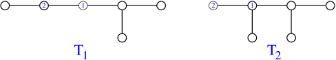
Figure 4: An example of $\mathsf{GTS}_{6}$

$$\begin{array}[]{|r||r|r||r|r||r|r|}\hline\cr&\lx@intercol\hfil\lambda_{\max}(\mathcal{L}_{T_{i}}^{q})\hfil\lx@intercol\vrule\lx@intercol\vrule\lx@intercol&\lx@intercol\hfil\lambda_{\min}(\mathcal{L}_{T_{i}}^{q})\hfil\lx@intercol\vrule\lx@intercol\vrule\lx@intercol&\lx@intercol\hfil\lambda_{a}(\mathcal{L}_{T_{i}}^{q})\hfil\lx@intercol\vrule\lx@intercol\\ \hline\cr q&\lambda_{\max}(\mathcal{L}_{T_{1}}^{q})&\lambda_{\max}(\mathcal{L}_{T_{2}}^{q})&\lambda_{\min}(\mathcal{L}_{T_{1}}^{q})&\lambda_{\min}(\mathcal{L}_{T_{2}}^{q})&\lambda_{a}(\mathcal{L}_{T_{1}}^{q})&\lambda_{a}(\mathcal{L}_{T_{2}}^{q})\\ \hline\cr\hline\cr 0.1&1.2017&1.2136&0.8208&0.8130&0.8890&0.9064\\ \hline\cr 0.5&2.2566&2.3660&0.3032&0.2929&0.5586&0.6340\\ \hline\cr 1.0&4.2143&4.5616&0.0000&0.0000&0.3249&0.4384\\ \hline\cr 1.5&6.9857&7.6742&-0.0864&-0.0981&0.2014&0.3258\\ \hline\cr 10.0&202.9803&211.9481&-0.0069&-0.0469&0.0070&0.0519\\ \hline\cr\end{array}$$

Table 1: The eigenvalues $\lambda_{max}(\mathcal{L}_{T_{i}}^{q})$, $\lambda_{min}(\mathcal{L}_{T_{i}}^{q})$ and $\lambda_{a}(\mathcal{L}_{T_{i}}^{q})$.

7 Eigenvalues of the $q,t$-Laplacian

Let $T$ be a tree with $n$ vertices. A generalization $\mathcal{L}_{T}^{q,t}$ was defined by Bapat and Sivasubramanian in [2]. Orient the edges of $T$ arbitrarily. Since $T$ is now directed, we use directed graph terminology for its arcs $(i,j)$. Define $\mathcal{L}_{T}^{q,t}=(\ell_{i,j})_{1\leq i,j\leq n}$ by $\ell_{i,j}=-q$, if $\{i,j\}$ is an edge $e$ in $T$ and the orientation of $e$ gives the arc $(i,j)$. If the orientation of $e=\{i,j\}$ gives the arc $(i,j)$, then, define $\ell_{j,i}=-t$. If $\{i,j\}=e$ with $i\neq j$ is not an edge in $T$, then, define $\ell_{i,j}=0$. Define $\ell_{i,i}=1+qt(d_{i}-1)$, where $d_{i}$ is the degree of the $i$-th vertex in $T$. It is easy to see that when $q=t$, $\mathcal{L}_{T}^{q,t}=\mathcal{L}_{T}^{q}$. Thus, $\mathcal{L}_{T}^{q,t}$ is a generalization of $\mathcal{L}_{T}^{q}$.

Let $T$ be a tree on $n$ vertices with $q,t$-Laplacian $\mathcal{L}_{T}^{q,t}$. For fixed but arbitrary $q,t\in\mathbb{C}$, let $f^{\mathcal{L}_{T}^{q,t}}(q,t,x)$ be the characteristic polynomial of $\mathcal{L}_{T}^{q,t}$ in three variables $q$, $t$ and $x$. Clearly Lemma 10 and Theorem 12 go through for $f^{\mathcal{L}_{T}^{q,t}}(q,t,x)$ when $q\neq 0$ and $t\neq 0$. In this case, it is easy to see that $y_{1}=0$, $y_{2}=1$, $y_{3}=-(x-1+qt)$ and $y_{4}=-1/qtx$.

We need the Interlacing Theorem for eigenvalues of Hermitian matrices to generalize Lemmas 19 and 20 to $\mathcal{L}_{T}^{q,t}$. Hence, we require $\mathcal{L}_{T}^{q,t}$ to be Hermitian. We see that the matrix $\mathcal{L}_{T}^{q,t}$ is Hermitian for all $q,t\in\mathbb{C}$ with $\mkern 1.5mu\overline{\mkern-1.5muq\mkern-1.5mu}\mkern 1.5mu=t$. When $\mkern 1.5mu\overline{\mkern-1.5muq\mkern-1.5mu}\mkern 1.5mu=t$, the proof of the $q,t$-version of the general lemma is identical to that of Lemma 10. Bapat and Sivasubramanian [2] proved that $\det(\mathcal{L}_{T}^{q,t})=1-qt.$ For $v\in T$, Nagar and Sivasubramanian [12] proved that $f^{\mathcal{L}_{T}^{q,t}|v}(q,t,0)=(-1)^{n-1}$ for all $q,t\in\mathbb{C}$. When $\mkern 1.5mu\overline{\mkern-1.5muq\mkern-1.5mu}\mkern 1.5mu=t$ in $\mathbb{C}\backslash\{0\}$, we get $qt=|q|^{2}>0$ and thus, Lemmas 19 and 20 go through for $\mathcal{L}_{T}^{q,t}$.

When $\mkern 1.5mu\overline{\mkern-1.5muq\mkern-1.5mu}\mkern 1.5mu=t\in\mathbb{C}$, Theorem 2 also goes through for the bivariate Laplacian matrix $\mathcal{L}_{T}^{q,t}$. Let $\lambda_{\min}(\mathcal{L}_{T}^{q,t})$, $\lambda_{a}(\mathcal{L}_{T}^{q,t})$ and $\lambda_{\max}(\mathcal{L}_{T}^{q,t})$ be the smallest, the second smallest and the largest eigenvalues of $\mathcal{L}_{T}^{q,t}$ respectively. We get the following result as a generalization of Theorem 2. As its proof is very similar to the proofs of Theorems 26, 29, 30 and 33, we omit and merely state the result.

Theorem 36

Let $T_{1}$ and $T_{2}$ be two trees on $n$ vertices such that $T_{2}$ covers $T_{1}$ in $\mathsf{GTS}_{n}$. Let $\mathcal{L}_{T_{1}}^{q,t}$ and $\mathcal{L}_{T_{2}}^{q,t}$ be the bivariate Laplacians of $T_{1}$ and $T_{2}$ respectively. Then, for $q,t\in\mathbb{C}$ with $\mkern 1.5mu\overline{\mkern-1.5muq\mkern-1.5mu}\mkern 1.5mu=t$, we have $\lambda_{\min}(\mathcal{L}_{T_{1}}^{q,t})\geq\lambda_{\min}(\mathcal{L}_{T_{2}}^{q,t})$, $\lambda_{\max}(\mathcal{L}_{T_{1}}^{q,t})\leq\lambda_{\max}(\mathcal{L}_{T_{2}}^{q,t})$ and $\lambda_{a}(\mathcal{L}_{T_{1}}^{q,t})\leq\lambda_{a}(\mathcal{L}_{T_{2}}^{q,t}).$

Thus, for all $\mkern 1.5mu\overline{\mkern-1.5muq\mkern-1.5mu}\mkern 1.5mu=t\in\mathbb{C}$, three eigenvalues of $\mathcal{L}_{T}^{q,t}$ exhibit monotonicity when we go up on $\mathsf{GTS}_{n}$. Moreover, for the largest and second smallest eigenvalues max-min pair is $(S_{n},P_{n})$ while for the smallest eigenvalue max-min pair is $(P_{n},S_{n})$. It is easy to determine the eigenvalues of $\mathcal{L}_{S_{n}}^{q,t}$ as done in Example 27. Thus, we get the following corollary of Theorem 36.

Corollary 37

Let $T$ be a tree on $n>2$ vertices with $q,t$-Laplacian $\mathcal{L}_{T}^{q,t}$. Then, for all $q,t\in\mathbb{C}$ with $\mkern 1.5mu\overline{\mkern-1.5muq\mkern-1.5mu}\mkern 1.5mu=t$, we have $\lambda_{a}(\mathcal{L}_{T_{1}}^{q,t})\leq 1$ and

$$\lambda_{\max}(\mathcal{L}_{T}^{q,t})\leq\frac{2+(n-2)qt+\sqrt{n^{2}q^{2}t^{2}+4(n-1)(1-qt)qt}}{2}.$$

When $q=1/t\in\mathbb{C}$ with $t\neq 0$ and $\mkern 1.5mu\overline{\mkern-1.5muq\mkern-1.5mu}\mkern 1.5mu\neq t$, the matrix $\mathcal{L}_{T}^{q,t}$ is no longer Hermitian but our result follows from Nagar and Sivasubramanian [12, Remark 34]. There it was proved that when $q=1/t\in\mathbb{C}$ with $t\neq 0$, $\det(xI-\mathcal{L}_{T}^{q,t})=\det(xI-L_{T})$, where $L_{T}$ is the Laplacian matrix of $T$. Thus, we have $\lambda_{\min}(\mathcal{L}_{T}^{q,t})=\lambda_{\min}(L_{T})$, $\lambda_{\max}(\mathcal{L}_{T}^{q,t})=\lambda_{\max}(L_{T})$ and $\lambda_{a}(\mathcal{L}_{T}^{q,t})=\lambda_{a}(L_{T})$. Moreover, we have $\lambda_{\max}(\mathcal{L}_{T}^{q,t})=\lambda_{\max}(L_{T})\leq n$ when $q=1/t\in\mathbb{C}$ with $t\neq 0$.

One special case of $\mathcal{L}_{T}^{q,t}$ is obtained when we set $q=\imath$ and $t=-\imath$, where $\imath=\sqrt{-1}$. In this case, the matrix $\mathcal{L}_{T}^{q,t}$ is the Hermitian positive semidefinite (see Bapat and Sivasubramanian [2]). The bivariate Laplacian matrix $\mathcal{L}_{T}^{q,t}$ is called the Hermitian Laplacian matrix of $T$ when $q=\imath$ and $t=-\imath$ defined by Yu and Qu [14]. In this case, we have both $\mkern 1.5mu\overline{\mkern-1.5muq\mkern-1.5mu}\mkern 1.5mu=t$ and $q=1/t$.

8 Eigenvalue monotonicity of $\mathsf{ED}_{T}$

Let $T$ be a tree on $n$ vertices with exponential distance matrix $\mathsf{ED}_{T}$. Let the eigenvalues of $\mathsf{ED}_{T}$ be $\lambda_{\max}(\mathsf{ED}_{T})=\lambda_{1}(\mathsf{ED}_{T})\geq\lambda_{2}(\mathsf{ED}_{T})\geq\cdots\geq\lambda_{n}(\mathsf{ED}_{T})=\lambda_{\min}(\mathsf{ED}_{T})$. When $q=\pm 1$, it is simple to see that the eigenvalues of $\mathsf{ED}_{T}$ are $n$ and $0$ with multiplicities $1$ and $n-1$ respectively. Thus, in this case, the eigenvalues of $\mathsf{ED}_{T}$ are constant on $\mathsf{GTS}_{n}$. By Lemmas 5 and 6, we see that $\mathsf{ED}_{T}$ is a positive definite matrix when $q\in\mathbbm{R}$ with $|q|<1$ and $\mathsf{ED}_{T}$ has exactly one positive eigenvalue when $q\in\mathbbm{R}$ with $|q|>1$. Let $\lambda_{\min}(\mathsf{ED}_{T})$, $\lambda_{\max}(\mathsf{ED}_{T})$ and $\lambda_{2}(\mathsf{ED}_{T})$ be the smallest, the largest and the second largest eigenvalues of $\mathsf{ED}_{T}$. The following theorem is our main result of this section.

Theorem 38

Let $T_{1}$ and $T_{2}$ be two trees with $n$ vertices such that $T_{2}$ covers $T_{1}$ in $\mathsf{GTS}_{n}$.

1. If $q\in\mathbbm{R}$ with $|q|<1$, then, $\lambda_{\min}(\mathsf{ED}_{T_{1}})\geq\lambda_{\min}(\mathsf{ED}_{T_{2}})$, $\lambda_{2}(\mathsf{ED}_{T_{1}})\geq\lambda_{2}(\mathsf{ED}_{T_{2}})$ and $\lambda_{\max}(\mathsf{ED}_{T_{1}})\leq\lambda_{\max}(\mathsf{ED}_{T_{2}}).$

2. If $q\in\mathbbm{R}$ with $|q|>1$, then, $\lambda_{\min}(\mathsf{ED}_{T_{1}})\leq\lambda_{\min}(\mathsf{ED}_{T_{2}})$, $\lambda_{2}(\mathsf{ED}_{T_{1}})\leq\lambda_{2}(\mathsf{ED}_{T_{2}})$ and $\lambda_{\max}(\mathsf{ED}_{T_{1}})\geq\lambda_{\max}(\mathsf{ED}_{T_{2}}).$

Proof:   When $q\in\mathbbm{R}$ with $|q|<1$, by using Lemma 6, all the eigenvalues of $\mathsf{ED}_{T_{1}}$ and $\mathsf{ED}_{T_{2}}$ are positive and they are

$$\lambda_{\max}(\mathsf{ED}_{T_{1}})=\frac{1-q^{2}}{\lambda_{\min}(\mathcal{L}_{T_{1}}^{q})} \geq \frac{1-q^{2}}{\lambda_{a}(\mathcal{L}_{T_{1}}^{q})}\geq\cdots\geq\frac{1-q^{2}}{\lambda_{1}(\mathcal{L}_{T_{1}}^{q})}=\frac{1-q^{2}}{\lambda_{\max}(\mathcal{L}_{T_{1}}^{q})}$$

$$\mbox{ and }\ \ \ \lambda_{\max}(\mathsf{ED}_{T_{2}})=\frac{1-q^{2}}{\lambda_{\min}(\mathcal{L}_{T_{2}}^{q})} \geq \frac{1-q^{2}}{\lambda_{a}(\mathcal{L}_{T_{2}}^{q})}\geq\cdots\geq\frac{1-q^{2}}{\lambda_{1}(\mathcal{L}_{T_{2}}^{q})}=\frac{1-q^{2}}{\lambda_{\max}(\mathcal{L}_{T_{2}}^{q})}$$ (29)

respectively. Similarly, when $|q|>1$, by Lemma 6, both the matrices $\mathsf{ED}_{T_{1}}$ and $\mathsf{ED}_{T_{2}}$ have exactly one positive eigenvalue and their eigenvalues are

$$\lambda_{\max}(\mathsf{ED}_{T_{1}})=\frac{1-q^{2}}{\lambda_{\min}(\mathcal{L}_{T_{1}}^{q})} \geq \frac{1-q^{2}}{\lambda_{\max}(\mathcal{L}_{T_{1}}^{q})}\geq\cdots\geq\frac{1-q^{2}}{\lambda_{n-1}(\mathcal{L}_{T_{1}}^{q})}=\frac{1-q^{2}}{\lambda_{a}(\mathcal{L}_{T_{1}}^{q})}$$

$$\mbox{ and }\ \ \ \lambda_{\max}(\mathsf{ED}_{T_{2}})=\frac{1-q^{2}}{\lambda_{\min}(\mathcal{L}_{T_{2}}^{q})} \geq \frac{1-q^{2}}{\lambda_{\max}(\mathcal{L}_{T_{2}}^{q})}\geq\cdots\geq\frac{1-q^{2}}{\lambda_{n-1}(\mathcal{L}_{T_{2}}^{q})}=\frac{1-q^{2}}{\lambda_{a}(\mathcal{L}_{T_{2}}^{q})}$$ (30)

respectively. Thus, by using (29), (30) and Theorem 2 the proof is complete.  

Thus, for all $q\in\mathbbm{R}$, three eigenvalues of $\mathsf{ED}_{T}$ exhibit monotonicity when we go up on $\mathsf{GTS}_{n}$ and max-min pair is either $(P_{n},S_{n})$ or $(S_{n},P_{n})$.

8.1 $q,t$-exponential distance matrix

We consider the bivariate exponential distance matrix $\mathsf{ED}_{T}^{q,t}$ of a tree $T$. Orient the tree $T$ as done in Section 7. Thus each directed arc $e$ of $E(T)$ has a unique reverse arc $e_{rev}$ and we assign a variable weight $w(e)=q$ and $w(e_{rev})=t$ or vice versa. If the path $P_{i,j}$ from vertex $i$ to vertex $j$ has the sequence of edges $P_{i,j}=(e_{1},e_{2},\ldots,e_{p})$, assign it weight $w_{i,j}=\prod_{e_{k}\in P_{i,j}}w(e_{k})$. Define $w_{i,i}=1$ for $i=1,2,\ldots,n$. Define the bivariate $q,t$-exponential distance matrix $\mathsf{ED}_{T}^{q,t}=(w_{i,j})_{1\leq i,j\leq n}$. Clearly, when $q=t$, we will have $\mathsf{ED}_{T}^{q,t}=\mathsf{ED}_{T}$. Bapat and Sivasubramanian in [2, Theorem 3.2] showed the following bivariate counterpart of Lemma 6.

Lemma 39 (Bapat and Sivasubramanian)

Let $T$ be a tree on $n$ vertices with $q,t$-Laplacian $\mathcal{L}_{T}^{q,t}$ and $q,t$-exponential distance matrix $\mathsf{ED}_{T}^{q,t}$. When $qt\neq 1$, then $(\mathsf{ED}_{T}^{q,t})^{-1}=\frac{1}{1-qt}\mathcal{L}_{T}^{q,t}.$ Moreover, $\frac{1-qt}{\lambda_{i}(\mathcal{L}_{T}^{q,t})}$ is an eigenvalue of $\mathsf{ED}_{T}^{q,t}$, where $\lambda_{i}(\mathcal{L}_{T}^{q,t})$ is an eigenvalue of $\mathcal{L}_{T}^{q,t}$.

From Theorem 36, it is easy to see that Theorem 38 goes through for the bivariate $q,t$-exponential distance matrix $\mathsf{ED}_{T}^{q,t}$ when $q,t\in\mathbb{C}$ with $\mkern 1.5mu\overline{\mkern-1.5muq\mkern-1.5mu}\mkern 1.5mu=t$ and $qt\not=1$.

References

[1]Bapat, R. B., Lal, A. K., and Pati, S.A -analogue of the distance matrix of a tree.
Linear Algebra and its Applications 416 (2006), 799–814.
[2]Bapat, R. B., and Sivasubramanian, S.The Product Distance Matrix of a Tree and a Bivariate
Zeta Function of a Graph.
Electronic Journal of Linear Algebra 23 (2012), 275–286.
[3]Bass, H.The Ihara-Selberg Zeta Function of a Tree Lattice.
International Journal of Math. 3 (1992), 717–797.
[4]Csikvári, P.On a conjecture of V. Nikiforov.
Discrete Mathematics 309, 13 (2009), 4522–4526.
[5]Csikvári, P.On a Poset of Trees.
Combinatorica 30 (2) (2010), 125–137.
[6]Csikvári, P.On a Poset of Trees II.
Journal of Graph Theory 74 (2013), 81–103.
[7]Foata, D., and Zeilberger, D.Combinatorial Proofs of Bass’s Evaluations of the
Ihara-Selberg Zeta function of a Graph.
Transactions of the AMS 351 (1999), 2257–2274.
[8]Godsil, C. D., and Royle, G.Algebraic Graph Theory.
Springer-Verlag New York, 2001.
[9]Horn, R. A., and Johnson, C. R.Matrix Analysis, 2 ed.
Cambridge University Press, 2012.
[10]Kelmans, A. K.On Graphs with Randomly Deleted Edges.
Acta Mathematica Acad. Sci. Hungarica 37 (1981), 77–88.
[11]Molitierno, J. J.Applications of Combinatorial Matrix Theory to Laplacian
Matrices of Graphs.
CRC Press, 2012.
[12]Nagar, M. K., and Sivasubramanian, S.Laplacian Immanantal polynomials and the GTS poset on trees.
Preprint available at arXiv: https://arxiv.org/abs/1710.02416
(2017).
[13]Satyanarayana, A., Schoppman, L., and Suffel, C. L.A Reliability-Improving Graph Transformation with
Applications to Network eliability.
Networks 22 (1992), 209–216.
[14]Yu, G., and Qu, H.Hermitian Laplacian matrix and positive of mixed graphs.
Applied Mathematics and Computation 269 (2015), 70–76.