Recent Results on Light-Meson Spectroscopy from COMPASS

Abstract:

The main goal of the spectroscopy program at COMPASS is to explore the light-meson spectrum below about $2\,\text{GeV}/c^{2}$ in diffractive production. Our flagship channel is the decay into three charged pions: $p+\pi^{-}\to\pi^{-}\pi^{-}\pi^{+}+p_{\text{recoil}}$, for which COMPASS has acquired the so far world’s largest dataset of roughly $50\,\text{M}$ exclusive events using an $190\,\text{GeV}/c$ $\pi^{-}$ beam. Based on this dataset, we performed an extensive partial-wave analysis. In order to extract the resonance parameters of the $\pi_{J}$ and $a_{J}$ states that appear in the $\pi^{-}\pi^{-}\pi^{+}$ system, we performed the so far largest resonance-model fit, using Breit-Wigner resonances and non-resonant contributions.

This method in combination with the high statistical precision of our measurement allows us to study ground and excited states. We have found an evidence of the $a_{1}(1640)$ and $a_{2}(1700)$ in our data, which are the first excitations of the $a_{1}(1260)$ and $a_{2}(1320)$, respectively. The relative strength of the excited states with respect to the corresponding ground state is larger in the $f_{2}(1270)\,\pi$ decay mode compared to the $\rho(770)\,\pi$ decay mode. We also study the spectrum of $\pi_{2}$ states in our data. Therefore, we simultaneously describe four $J^{PC}=2^{-+}$ waves in the resonance-model fit by using three $\pi_{2}$ resonances, the $\pi_{2}(1670)$, the $\pi_{2}(1880)$, and the $\pi_{2}(2005)$. Within the limits of our model, we can conclude that the $\pi_{2}(2005)$ is required to describe all four $2^{-+}$ waves properly.

1 Light-meson spectroscopy at COMPASS

COMPASS is a fixed-target multi-purpose experiment located at CERN (SPS). Positive and negative secondary hadron beams with momenta of $190\text{\,}\mathrm{GeV}\text{\,}{\mathrm{\text{$c$}}}^{-1}$ or a tertiary muon beam of $160\text{\,}\mathrm{GeV}\text{\,}{\mathrm{\text{$c$}}}^{-1}$ can impinge various types of targets. The final-state particles are detected by a two-stage magnetic spectrometer, which has a large acceptance over a broad kinematic range.

The main goal of the COMPASS spectroscopy program is to study the light-meson spectrum up to about $2\text{\,}\mathrm{GeV}\text{\,}{\mathrm{\text{$c$}}}^{-2}$. At COMPASS, these light mesons are produced in diffractive scattering of the $190\text{\,}\mathrm{GeV}\text{\,}{\mathrm{\text{$c$}}}^{-1}$ negative hadron beam, which is mainly composed out of negative pions, is scattered off a liquid-hydrogen target. In these reactions, we can study $a_{J}$- and $\pi_{J}$-like mesons. Due to their very short lifetime, we observe them only in the decay into quasi-stable final-state particles. Our flagship channel is the decay into three charged pions: $\pi^{-}+p\to{\pi^{-}\pi^{-}\pi^{+}}+p_{\text{recoil}}$. COMPASS has acquired the so far world’s largest dataset of this channel of about $50\text{\,}\mathrm{M}$ exclusive events, which allows us to apply novel analysis methods [1].

2 Analysis method

2.1 Partial-wave decomposition

We employ the method of partial-wave analysis in a two-step approach. In the first step, called partial-wave decomposition, data are decomposed into the different contributions from the partial waves [1]. Therefore, we parametrize the intensity distribution $\mathcal{I}(\tau)$ of the ${\pi^{-}\pi^{-}\pi^{+}}$ final state in turns of five-dimensional phase-space variables that are represented by $\tau$. Using the isobar approach, $\mathcal{I}(\tau)$ is modeled as a coherent sum of partial-wave amplitudes, which are defined by the $3\pi$ quantum numbers and the decay path represented by $\alpha={J}^{{PC}}\,\allowbreak{M}^{\varepsilon}\,\allowbreak{\zeta}\,\pi\,{L}$:

$$\mathcal{I}(\tau;m_{3\pi},{t^{\prime}})=\left|\sum\limits_{\alpha}^{\text{waves}}{\mathcal{T}_{\alpha}(m_{3\pi},{t^{\prime}})}\,{\psi_{\alpha}(\tau;m_{3\pi},{t^{\prime}})}\right|^{2}.$$

The decay amplitudes $\psi_{\alpha}$ can be calculated. This allows us to extract the partial-wave amplitudes $\mathcal{T}_{\alpha}$, which determine the strength and phase of each wave, from the data by an unbinned maximum-likelihood fit, which is performed in narrow bins of the three-pion mass $m_{3\pi}$.

The large size of the dataset allows us to bin our data in the squared four-momentum transfer ${t^{\prime}}$ as well. By performing the partial-wave decomposition independently in $100$ narrow $m_{3\pi}$ bins and $11$ ${t^{\prime}}$ bins in the range $0.5<m_{3\pi}<$2.5\text{\,}\mathrm{GeV}\text{\,}{\mathrm{\text{$c$}}}^{-2}$$ and $0.1<{t^{\prime}}<$1.0\text{\,}\mathrm{(GeV/)^{2}}$$, we extract simultaneously the $m_{3\pi}$ and ${t^{\prime}}$ dependence of the partial-wave amplitudes from the data.

2.2 Resonance-model fit

At the second step of this analysis, called resonance-model fit, we parameterize the $m_{3\pi}$ dependence of the partial-wave amplitudes in order to extract the masses and widths of resonances appearing in the ${\pi^{-}\pi^{-}\pi^{+}}$ system. Details can be found in Refs. [2, 3]. We model the amplitude for the wave $\alpha$ as a coherent sum over components $k$ that we assume to contribute to this wave:

$$\mathcal{T}_{\alpha}(m_{3\pi},{t^{\prime}})=\smashoperator[r]{\sum_{k_{\alpha}}^{}}\mathcal{C}^{k_{\alpha}}_{\alpha}({t^{\prime}})\cdot\mathcal{D}^{k_{\alpha}}(m_{3\pi},{t^{\prime}};\zeta_{k}).$$

The dynamical amplitudes $\mathcal{D}^{k}(m_{3\pi},{t^{\prime}};\zeta_{k})$ represent the resonant and non-resonant components. We use relativistic Breit-Wigner amplitudes for resonances and a phenomenological parameterization for the non-resonant terms. Each dynamical amplitude is multiplied by a coupling amplitude $\mathcal{C}^{k_{\alpha}}_{\alpha}({t^{\prime}})$, which determines the strength and phase with which each component contributes to the corresponding wave. We use independent coupling amplitudes for each ${t^{\prime}}$ bin. Thus, also in this analysis step, we impose no model for the ${t^{\prime}}$ dependence of the components. We simultaneously describe all $11$ ${t^{\prime}}$ bins in one resonance-model fit, keeping the mass and width parameters of each resonance component the same in each ${t^{\prime}}$ bin. In this way, our ${t^{\prime}}$-resolved analysis gives us an additional dimension of information, which helps to separate resonant from non-resonant components better.

Our two-step approach allows us to select a subset of waves to be included in the resonance-model fit. In this analysis, we select a subset of 14 out of the 88 partial waves with $J^{PC}=0^{-+}$, $1^{++}$, $1^{-+}$, $2^{++}$, $2^{-+}$, and $4^{++}$ quantum numbers. This subset accounts for about $60\text{\,}\mathrm{\char 37\relax}$ of the total intensity. The 14 waves are parameterized by 11 resonances; $\pi(1800)$, $a_{1}(1260)$, $a_{1}(1420)$, $a_{1}(1640)$, $\pi_{1}(1600)$, $a_{2}(1320)$, $a_{2}(1700)$, $\pi_{2}(1670)$, $\pi_{2}(1880)$, $\pi_{2}(2005)$, and $a_{4}(2040)$; and 14 non-resonant terms.

Many systematic effects might influence the fit result. To investigate these effects we performed more than 200 systematic studies to improve our model, to test the evidence for some resonance signals in our data, and to determine systematic uncertainties of extracted resonance parameters.

3 Results of the resonance-model fit

In the following subsections we present selected preliminary results for resonances with $J^{PC}=2^{++}$, $1^{++}$, and $2^{-+}$ quantum numbers. As the statistical uncertainties are at least one order of magnitude smaller than the systematic ones, we quote only systematic uncertainties. All results of the resonance-model fit are discussed in Ref. [2] and will be published in Ref. [3].

3.1 $\mathbf{J^{PC}=2^{++}}$ resonances

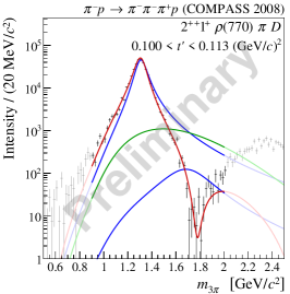
(a)

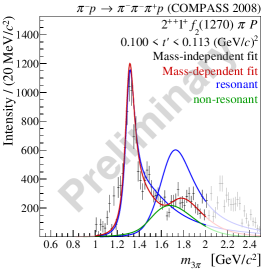
(b)

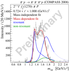
(c)

Figure 1: (a) intensity distributions of the ${2}^{{++}}\,\allowbreak{1}^{+}\,\allowbreak{\rho(770)}\,\pi\,{D}$ wave in the lowest ${t^{\prime}}$ bin in log-scale. (b) and (c) intensity distributions of the ${2}^{{++}}\,\allowbreak{1}^{+}\,\allowbreak{f_{2}(1270)}\,\pi\,{P}$ wave in the lowest and highest ${t^{\prime}}$ bin, respectively. The data points show the result of the partial-wave decomposition. Errors are statistical only. The red curves represent the resonance model. The blue curves represent the resonances. The green curves represent the non-resonant components. The extrapolations beyond the $m_{3\pi}$ fit range are shown in lighter colors.

The ${2}^{{++}}\,\allowbreak{1}^{+}\,\allowbreak{\rho(770)}\,\pi\,{D}$ wave exhibits a clear narrow peak in the mass region of the well-known $a_{2}(1320)$ resonance (see Figure 1a). As it is expected, this peak is mainly described by the $a_{2}(1320)$ component with only small contributions from other components. Therefore, our estimate for the $a_{2}(1320)$ mass of $1314.2\,^{+1.0}_{-3.1}\,$\mathrm{MeV}\text{\,}{\mathrm{\text{$c$}}}^{-2}$$ and width of $106.7\,^{+3.5}_{-2.4}\,$\mathrm{MeV}\text{\,}{\mathrm{\text{$c$}}}^{-2}$$ is stable with respect to systematic effects and in agreement with previous measurements.

In addition to the $a_{2}(1320)$ peak, the ${2}^{{++}}\,\allowbreak{1}^{+}\,\allowbreak{\rho(770)}\,\pi\,{D}$ wave shows some evidence for a potential $a_{2}(1700)$ excited state. In the low ${t^{\prime}}$-region, the observed dip at $1.8\text{\,}\mathrm{GeV}\text{\,}{\mathrm{\text{$c$}}}^{-2}$ is reproduced well as a destructive interference between the $a_{2}(1700)$ component and the other components in this wave. The ${2}^{{++}}\,\allowbreak{1}^{+}\,\allowbreak{f_{2}(1270)}\,\pi\,{P}$ wave shows the strongest evidence for the $a_{2}(1700)$. The shape of its intensity distribution is modulated strongly with ${t^{\prime}}$ (see Figures 1b and 1c), which is reproduced well by the model as a change of the interference pattern between the $a_{2}(1700)$ and the other components in this wave. The measured $a_{2}(1700)$ mass and width parameters of $1674\,^{+140}_{-32}\,$\mathrm{MeV}\text{\,}{\mathrm{\text{$c$}}}^{-2}$$ and $435\,^{+50}_{-15}\,$\mathrm{MeV}\text{\,}{\mathrm{\text{$c$}}}^{-2}$$ show larger systematic uncertainties, as the $a_{2}(1700)$ is a small signal compared to the dominant $a_{2}(1320)$. The PDG [4] lists the $a_{2}(1700)$ as “omitted from summary table” [4]. The world average for its mass is in agreement with our observation, but our estimate for the width is $240\text{\,}\mathrm{MeV}\text{\,}{\mathrm{\text{$c$}}}^{-2}$ larger than the world average. A recent analysis of COMPASS data on the $\eta\pi$ final state using an analytic model based on the principles of the relativistic $S$-matrix also obtained a smaller width for the $a_{2}(1700)$ of $280\pm 10(\text{stat.})\pm 70(\text{sys.})\,$\mathrm{MeV}\text{\,}{\mathrm{\text{$c$}}}^{-2}$$ [5]. However, the authors of Ref. [5] only fitted the intensity spectra. In contrast to our analysis, the relative phase information and the evolution with ${t^{\prime}}$ were not taken into account.

3.2 $\mathbf{J^{PC}=1^{++}}$ resonances

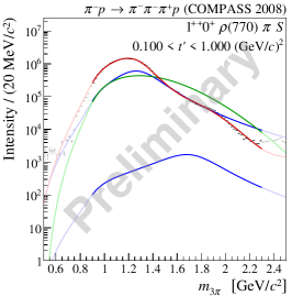
(a)

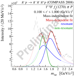
(b)

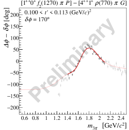
(c)

Figure 2: ${t^{\prime}}$-summed intensity distributions of the (a) ${1}^{{++}}\,\allowbreak{0}^{+}\,\allowbreak{\rho(770)}\,\pi\,{S}$ and the (b) ${1}^{{++}}\,\allowbreak{0}^{+}\,\allowbreak{f_{2}(1270)}\,\pi\,{P}$ waves. (c) shows the relative phase of the ${1}^{{++}}\,\allowbreak{0}^{+}\,\allowbreak{f_{2}(1270)}\,\pi\,{P}$ wave w.r.t. the ${4}^{{++}}\,\allowbreak{1}^{+}\,\allowbreak{\rho(770)}\,\pi\,{G}$ wave. Same color code as in Figure 1 is used.

The ${1}^{{++}}\,\allowbreak{0}^{+}\,\allowbreak{\rho(770)}\,\pi\,{S}$ wave contributes about $30\text{\,}\mathrm{\char 37\relax}$ to the total intensity and is the dominant signal in our data. It exhibits a broad peak in the intensity distribution at about $1.2\text{\,}\mathrm{GeV}\text{\,}{\mathrm{\text{$c$}}}^{-2}$ (see Figure 2a). This broad peak is described by the $a_{1}(1260)$ component and the non-resonant component of similar intensity. The resonance model cannot describe the details of the intensity spectrum of the ${1}^{{++}}\,\allowbreak{0}^{+}\,\allowbreak{\rho(770)}\,\pi\,{S}$ wave within the small statistical uncertainties properly. This is mainly due to the large contribution of the non-resonant component, in combination with our lack of accurate knowledge about the non-resonant shape. This also leads to large systematic uncertainties of the measured $a_{1}(1260)$ mass and width of $1298\,^{+13}_{-22}\,$\mathrm{MeV}\text{\,}{\mathrm{\text{$c$}}}^{-2}$$ and $400\,^{+0}_{-100}\,$\mathrm{MeV}\text{\,}{\mathrm{\text{$c$}}}^{-2}$$, respectively, which are in agreement with previous measurements.

Similar to the $2^{++}$ waves, we observe the evidence for a potential $a_{1}(1640)$ in the high-mass tail of the $a_{1}(1260)$, visible as a shoulder at about $1.8\text{\,}\mathrm{GeV}\text{\,}{\mathrm{\text{$c$}}}^{-2}$ in the intensity spectrum of the ${1}^{{++}}\,\allowbreak{0}^{+}\,\allowbreak{\rho(770)}\,\pi\,{S}$ wave. The strongest evidence for the $a_{1}(1640)$ is observed in the ${1}^{{++}}\,\allowbreak{0}^{+}\,\allowbreak{f_{2}(1270)}\,\pi\,{P}$ wave. It shows as a clear peak at about $1.8\text{\,}\mathrm{GeV}\text{\,}{\mathrm{\text{$c$}}}^{-2}$ (see Figure 2b) in combination with a rising phase motion in this mass region (see Figure 2c). Both are reproduced well by the resonance model. Our estimate for the $a_{1}(1640)$ parameters are $m_{0}=1690\,^{+40}_{-70}\,$\mathrm{MeV}\text{\,}{\mathrm{\text{$c$}}}^{-2}$$ and $\Gamma_{0}=534\,^{+124}_{-20}\,$\mathrm{MeV}\text{\,}{\mathrm{\text{$c$}}}^{-2}$$. The PDG lists the $a_{1}(1640)$ as “omitted from summary table”. The world average for the mass is in agreement with our observation, but our estimate for the width is $280\text{\,}\mathrm{MeV}\text{\,}{\mathrm{\text{$c$}}}^{-2}$ larger than the world average.

3.3 $\mathbf{J^{PC}=2^{-+}}$ resonances

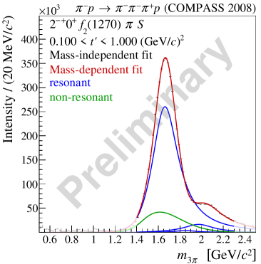
(a)

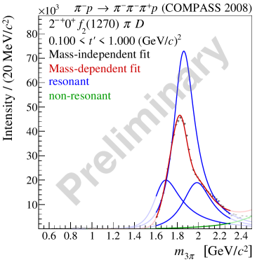
(b)

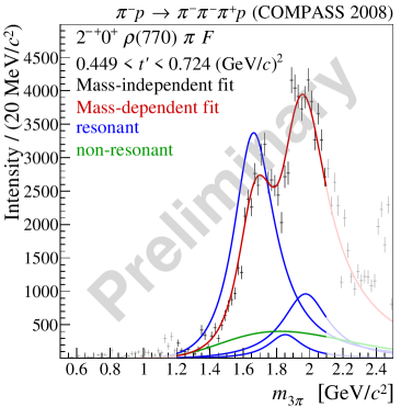
(c)

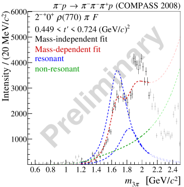
(d)

Figure 3: ${t^{\prime}}$-summed intensity distributions of the (a) ${2}^{{-+}}\,\allowbreak{0}^{+}\,\allowbreak{f_{2}(1270)}\,\pi\,{S}$ and (b) the ${2}^{{-+}}\,\allowbreak{0}^{+}\,\allowbreak{f_{2}(1270)}\,\pi\,{D}$ waves. (c) and (d) show the ${2}^{{-+}}\,\allowbreak{0}^{+}\,\allowbreak{\rho(770)}\,\pi\,{F}$ partial-wave intensity distribution in the second highest ${t^{\prime}}$ bin. The curves in (c) show the standard fit, the dashed curves in (d) the result fo a fit without the $\pi_{2}(2005)$ component. Same color code as in Figure 1 is used.

We include four partial waves with $J^{PC}=2^{-+}$ into the resonance-model fit, each of which is parameterized by three resonance components and a non-resonant component. The ${2}^{{-+}}\,\allowbreak{0}^{+}\,\allowbreak{f_{2}(1270)}\,\pi\,{S}$ wave is the largest of the four. It exhibits a striking peak at about $1.65\text{\,}\mathrm{GeV}\text{\,}{\mathrm{\text{$c$}}}^{-2}$ (see Figure 3a). This peak is reproduced well by a dominant contribution of the $\pi_{2}(1670)$ component.

The ${2}^{{-+}}\,\allowbreak{0}^{+}\,\allowbreak{f_{2}(1270)}\,\pi\,{D}$ wave exhibits a striking peak as well. However, not at $1.65\text{\,}\mathrm{GeV}\text{\,}{\mathrm{\text{$c$}}}^{-2}$, but at about $1.8\text{\,}\mathrm{GeV}\text{\,}{\mathrm{\text{$c$}}}^{-2}$ (see Figure 3b). The peak is described mainly by the $\pi_{2}(1880)$ component. The low- and high-mass tails of the peak are described as an interference effect among the $\pi_{2}(1880)$, the $\pi_{2}(1670)$, or the $\pi_{2}(2005)$ components.

The ${2}^{{-+}}\,\allowbreak{0}^{+}\,\allowbreak{\rho(770)}\,\pi\,{F}$ wave shows the strongest evidence for the $\pi_{2}(2005)$. We observe a double-peak structure (see Figure 3c). The lower-lying peak is at about $1.65\text{\,}\mathrm{GeV}\text{\,}{\mathrm{\text{$c$}}}^{-2}$ and is mainly described by the $\pi_{2}(1670)$ component. The higher-lying peak is at about $2\text{\,}\mathrm{GeV}\text{\,}{\mathrm{\text{$c$}}}^{-2}$ and is described by the $\pi_{2}(2005)$ component. The relative strength between the peaks changes strongly with ${t^{\prime}}$. In order to study the significance of the $\pi_{2}(2005)$ signal in our data, we performed a systematic study, in which we removed the $\pi_{2}(2005)$ component from the resonance model, such that all four $2^{-+}$ waves are parameterized only by the $\pi_{2}(1670)$ and $\pi_{2}(1880)$ components and the non-resonant components. The result of this study is shown in Figure 3d. The $2\text{\,}\mathrm{GeV}\text{\,}{\mathrm{\text{$c$}}}^{-2}$ mass region cannot be reproduced well without the $\pi_{2}(2005)$ component. Furthermore, the $\pi_{2}(1880)$ width increases in this study by about $100\text{\,}\mathrm{MeV}\text{\,}{\mathrm{\text{$c$}}}^{-2}$, and would be in contradiction to all previous observations.

4 Discussion

We have performed the so far largest resonance-model fit simultaneously and consistently describing 14 partial waves by a single model. The huge amount of information condensed in this fit, in combination with the information from the ${t^{\prime}}$-resolved analysis allows us to study ground as well as excited states. We observe signals of the $a_{1}(1640)$ and $a_{2}(1700)$, which are the first excitations of the $a_{1}(1260)$ and $a_{2}(1320)$,respectively. As both states appear in the high-mass tails of the dominant ground states, we extract their parameters with large systematic uncertainties. Our estimate for their widths is systematically larger in comparison to previous observations, which might indicate an imperfect separation of the wave components in the corresponding mass regions. We also observe, that the $\rho(770)$ $\pi$ decay mode of the $1^{++}$ and $2^{++}$ waves is dominated by the ground states, while the excited states are more dominant in the $f_{2}(1270)$ $\pi$ decay mode. Also in the $2^{-+}$ waves we observe that the different resonances contribute with different relative strength to the different decay modes. Furthermore, we require a second excited state, the $\pi_{2}(2005)$, to describe properly all four $2^{-+}$ partial waves simultaneously. To reduce the systematic uncertainties and further clarify the existence of higher states, models that are based on the principles of unitarity and analyticity are mandatory, especially in waves where the non-resonant contributions are important.

References

- [1] C. Adolph. et al. [COMPASS Collaboration] “Resonance production and -wave in at ” In Physical Review D 95, 2017, pp. 032004
- [2] Stefan Wallner “Extraction of Resonance Parameters of Light Meson Resonances in the Charged Three-Pion Final State at the COMPASS Experiment (CERN)”, 2015 URL: http://wwwcompass.cern.ch/compass/publications/theses/2015_dpl_wallner.pdf
- [3] C. Adolph. et al. [COMPASS Collaboration] “Light isovector resonances in at ” to be published, 2018
- [4] K.A. Olive “Review of Particle Physics” In Chinese Physics C 40, 2016, pp. 100001
- [5] A. Jackura et al. [JPAC and COMPASS Collaboration] “New analysis of tensor resonances measured at the COMPASS experiment” In submitted to Phys. Lett. B, 2017 arXiv:1707.02848 [hep-ph]