Magnetotransport properties of ${\rm 8-Pmmn}$ borophene: effects of Hall field and strain

Abstract

The polymorph of ${\rm 8-Pmmn}$ borophene is an anisotropic Dirac material with tilted Dirac cones at two valleys. The tilting of the Dirac cones at two valleys are in opposite directions, which manifests itself via the valley dependent Landau levels in presence of an in-plane electric field (Hall field). The valley dependent Landau levels cause valley polarized magnetotransport properties in presence of the Hall field, which is in contrast to the monolayer graphene with isotropic non-tilted Dirac cones. The longitudinal conductivity and Hall conductivity are evaluated by using linear response theory in low temperature regime. An analytical approximate form of the longitudinal conductivity is also obtained. It is observed that the tilting of the Dirac cones amplifies the frequency of the longitudinal conductivity oscillation (Shubnikov-de Haas). On the other hand, the Hall conductivity exhibits graphene-like plateaus except the appearance of valley dependent steps which are purely attributed to the Hall field induced lifting of the valley degeneracy in the Landau levels. Finally we look into the different cases when the Hall field is applied to the strained borophene and find that valley dependency is fully dominated by strain rather than Hall field. Another noticeable point is that if the real magnetic field is replaced by the strain induced pseudo magnetic field then the electric field looses its ability to cause valley polarized transport.

I Introduction

The discovery of the atomically thin two dimensional (2D) material-grapheneCastro Neto et al. (2009); Sarma et al. (2011), has received much attention in the last decade because of its unique physical properties as well as possible future applications. The electronic properties of the graphene are governed by its massless linear band dispersion rather than usual parabolic. Moreover, another intriguing feature of the graphene is that the bulk consists two inequivalent valleys ($K$ and $K^{\prime}$) in the first Brillouin zone of its band structure, which are the key ingredient for the newly emerged field -Valleytronics Schaibley et al. (2016); Ang et al. (2017); Kundu et al. (2016), just like Spintronics Žutić et al. (2004); Sinova et al. (2015); Schliemann (2017) based on spin. Apart from the graphene, similar materials like siliceneLalmi et al. (2010); Vogt et al. (2012); Drummond et al. (2012); Liu et al. (2011), transition-metal dichalcogenidesXiao et al. (2012); Mak et al. (2010), exhibiting linear dispersion with strong spin-orbit coupling, have also been extensively considered from the theoretical as well as experimental fronts. The polymorph of borophene which exhibits anisotropic tilted Dirac cones in its band structure (named as ${\rm 8-Pmmn}$) is the latest member to the family of Dirac materials Zhou et al. (2014) after the experimental realizationFeng et al. (2017) of it. A detailed ab-initio propertiesLopez-Bezanilla and Littlewood (2016) of this material was also addressed recently. Similar to the strained graphenePereira and Castro Neto (2009a), a pseudo magnetic field has also been predicted in ${\rm 8-Pmmn}$ boropheneZabolotskiy and Lozovik (2016) under the influence of strain. Very recently, several theoretical investigations on optical properties like anisotropic plasmonsSadhukhan and Agarwal (2017), effects of particle-hole symmetry breaking in optical conductivityVerma et al. (2017) and Drude weight have been reported.

The magnetotresistivity measurement of a 2D electronic system is one of the most appreciated method to probe the system. The application of a perpendicular uniform magnetic field to the 2D electronic systems quantizes the electronic energy spectrum i.e., forms Landau levels (LLs). The LLs can be realized by oscillatory longitudinal conductivity with inverse magnetic field known as Shubnikov-de Haas (SdH) oscillationsFeng and Jin (2005); Imry . On the other hand, the off-diagonal terms in conductivity tensor becomes quantized due to the incomplete cyclotron orbits along the opposite transverse edges of the systemFeng and Jin (2005); Imry . The quantum Hall conductivity in graphene Gusynin and Sharapov (2005); Zheng and Ando (2002); Krstajić and Vasilopoulos (2012) is $\sigma_{xy}=4(n+1/2)e^{2}/h$ with $n=0,1,2,3..$, which is in contrast to usual 2D electron gas where $\sigma_{xy}=2(n+1)e^{2}/h$. Note that ‘e’ and ‘h’ are the electronic charge and the Planck constant, respectively. Apart from the graphene, the magnetoconductivity has been extensively studied in siliceneShakouri et al. (2014); Tahir and Schwingenschlögl (2013), topological insulatorsTahir and Schwingenschlögl (2012); Shakouri and Peeters (2015); Büttner et al. (2011); Zhang et al. (2015),phosphoreneZhou et al. (2015); Ghazaryan and Chakraborty (2015); Mogulkoc et al. (2017), staneneMogulkoc et al. (2016) and molybdenum disulfideTahir et al. (2016); Islam and Benjamin etc. Apart from the modulation induced Weiss oscillations in ${\rm 8-Pmmn}$ boropheneIslam and Jayannavar (2017), several theoretical investigationsProskurin et al. (2015); Morinari et al. (2009); Kobayashi et al. (2008) of magnetotransport properties in 2D Dirac materials with tilted Dirac cones have been also carried out. However, so far no attempt has been made in such material with tilted Dirac cones to modulate valley degree of freedom in the integer quantum Hall effect and the longitudinal conductivity by applying an in-plane electric field (Hall field) in presence of randomly scattered charge impurities. In this work, we rectify this anomaly and try to obtain valley dependent magnetoconductivity in presence of a Hall field.

In this work, we investigate the quantum magnetotransport properties in presence of a Hall field in low temperature regime by using the linear response theory. One of the key issues of the valleytronics (spintronics) is how to control or modulate the two valleys (spin) independently by means of external parameters. We aim to modulate the valley dependency of the magnetoconductivity by applying an in-plane electric field. We should mention here that such valley dependent transport can be found in other 2D Dirac materials tooYarmohammadi (2017); Hoi et al. (2017, 2018); Shirzadi and Yarmohammadi . However, in those materials the presence of a strong spin-orbit interaction term removes the spin/valley degeneracy in its band structure. Assuming the elastic or quasi-elastic scattering of electron by charge impurities, scattered randomly in the system, we calculate the longitudinal and the Hall conductivity. The longitudinal conductivity shows SdH oscillations with the inverse magnetic field. The frequency of the SdH oscillations is amplified by the tilting of the Dirac cones. We also notice that the quantum Hall conductivity exhibits Hall plateaus of the form of $\sigma_{xy}=2(n+1/2)e^{2}/h$, exactly similar to the case of graphene in each valley. However, a valley separation is visible at the Hall steps and the SdH oscillations peaks due to the presence of the Hall field. This is in contrast to the non-tilted isotropic Dirac material like grapheneKrstajić and Vasilopoulos (2011), where magnetotransport properties are not sensitive to the valley index in the presence of a Hall field.

The paper is organized as follows. In Sec. II, we introduce the low energy effective Hamiltonian and discuss the lifting of the valley degeneracy in LLs in presence of a Hall field. The Sec. III is devoted to calculate different components of the magnetoconductivity tensor and analyze the results. Finally, we summarize and conclude in Sec. V.

II Model Hamiltonian and Landau level formation

In this section, we derive LLs and corresponding eigen states. We start with the low-energy single-particle effective model Hamiltonian for the tilted anisotropic Dirac cones asZabolotskiy and Lozovik (2016); Sadhukhan and Agarwal (2017)

$$H=\xi(v_{x}p_{x}\sigma_{x}+v_{y}p_{y}\sigma_{y}+v_{t}p_{y}\mathbb{1}),$$ (1)

where $\xi=+(-)$ denotes the valley $K(K^{\prime})$, three velocities are given by $\{v_{x},v_{y},v_{t}\}=\{0.86,0.69,0.32\}$ in units of $v_{0}=10^{6}$ m/sec. Also, ${\bf\sigma\equiv(\sigma_{x},\sigma_{y})}$ are the pseudo Pauli matrices and $\mathbb{1}$ is identity matrix. Note that unlike non-tilted isotropic Dirac cones in graphene, the velocities along $x$ and $y$ direction are not identical. The above Hamiltonian can be diagonalized to obtain the energy dispersion as

$${\varepsilon}_{\lambda,k}^{\xi}=\xi\hbar v_{t}k_{y}+\lambda\hbar\sqrt{v_{x}^{2}k_{x}^{2}+v_{y}^{2}k_{y}^{2}},$$ (2)

where $\lambda=\pm$ denotes the band index and ${\bf k}=\{k_{x},k_{y}\}$ is the $2$D momentum vector.

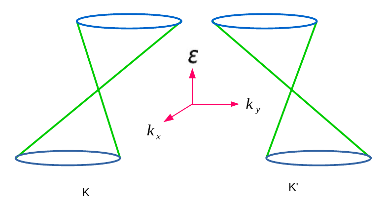
Figure 1: (Color online) A schematic sketch of the energy band dispersion in k-space, representing Eq. (2) in valley K and K^′.

This energy dispersion is shown schematically in Fig. (1), which is tilted along $k_{y}$-direction due to the presence of $v_{t}$ term. However, the tilting of the two Dirac cones at the two valleys is in opposite directions. Note that the tilting of the Dirac cones breaks the particle-hole symmetry in the $8-Pmmn$ borophene.

II.0.1 Inclusion of crossed electric and magnetic field

To include the effects of perpendicular magnetic field (${\bf B}=B\hat{z}$) in the low energy single-electron effective Hamiltonian of borophene, lying in the $x$-$y$ plane, we use the Landau-Peierls substitution, ${\bf p}\rightarrow{\bf p+eA}$, as

$$\mathcal{H}=\xi[v_{x}p_{x}\sigma_{x}+v_{y}(p_{y}+eBx)\sigma_{y}+v_{t}(p_{y}+eBx)\mathbb{1}]$$ (3)

under the Landau gauge ${\bf A}=(0,xB,0)$. Here, $A$ represents the magnetic vector potential. The effect of an in-plane uniform real electric field ($E_{r}$) can be included by adding a potential energy $U=eE_{r}x\mathbb{1}$ to the Hamiltonian as

$$\mathcal{H}_{e}=eE_{r}x\mathbb{1}+\xi[v_{x}p_{x}\sigma_{x}+v_{y}(p_{y}+eBx)\sigma_{y}+v_{t}(p_{y}+eBx)\mathbb{1}],$$ (4)

The Hamiltonian is translationally invariant along the $y$-direction as $[\mathcal{H}_{e},p_{y}]=0$, which allows the electron to be governed by the wave function $\Psi(x,y)\sim e^{ik_{y}y}\phi(x)$. Using this fact, the eigen value problem reduces to

$$\mathcal{H}_{0}\phi(x)={\varepsilon}\phi(x),$$ (5)

where

$$\mathcal{H}_{0}=\frac{\hbar v_{e}^{\xi}}{l_{c}}X\mathbb{1}+\xi\left\{\frac{\hbar v_{c}}{l_{c}}\left[\sqrt{\frac{v_{x}}{v_{y}}}\sigma_{x}P+\sqrt{\frac{v_{y}}{v_{x}}}\sigma_{y}X\right]\right\},$$ (6)

and

$${\varepsilon}=E+\hbar v_{e}k_{y},$$ (7)

where $v_{e}^{\xi}=v_{e}+\xi v_{t}$ with $v_{e}=E_{r}/B$, the magnetic length $l_{c}=\sqrt{\hbar/eB}$, the dimensionless x-component of momentum operator $P=-i\partial/\partial(x/l_{c})$, position operator $X=(x+x_{0})/l_{c}$ with the center of cyclotron orbit is at $x=-x_{0}=-k_{y}l_{c}^{2}$ and $v_{c}=\sqrt{v_{x}v_{y}}$. Apart from the velocity anisotropy inside the third bracket in Eq. (6), the above Hamiltonian is very much identical to the case of monolayer graphene under crossed electric and magnetic fieldLukose et al. (2007). The first term acts as a pseudo in-plane effective electric field ($E_{eff}=\hbar v_{e}^{\xi}/(el_{c}^{2})$). Now Eq. (6) can be re-written as

$$H_{\xi}=e\frac{E_{eff}}{\sqrt{2}}(a+a^{\dagger})\mathbb{1}+\xi\hbar\omega_{c}\left[\begin{array}[c]{c c}0&-ia\\ ia^{\dagger}&0\end{array}\right],$$ (8)

where $\omega_{c}(=v_{c}/l_{c})$ is the cyclotron frequency and ladder operators are defined as: $a=(\tilde{X}+i\tilde{P})/\sqrt{2}$ and $a^{\dagger}=(\tilde{X}-i\tilde{P})/\sqrt{2}$. Here, $\tilde{X}=\sqrt{\frac{v_{y}}{v_{x}}}X$ and $\tilde{P}=\sqrt{\frac{v_{x}}{v_{y}}}P$, satisfying the commutator relation $[\tilde{X},\tilde{P}]=i$. In absence of $E_{eff}$, the above Hamiltonian can be diagonalized to obtain graphene-like LLs (for $n\geq 0$)

$${\varepsilon}_{\zeta}=\lambda\hbar\omega_{c}\sqrt{2n},$$ (9)

with $\zeta=\{n,\xi,k_{y}\}$ and eigenfunctions as

$$\Psi_{\zeta}({\bf r})=\frac{e^{ik_{y}y}}{\sqrt{2L_{y}}}\left[\begin{array}[c]{c}\xi\lambda\phi_{n-1}(X)\\ i\phi_{n}(X)\end{array}\right],$$ (10)

where $\phi_{n}(X)$ is the well known simple harmonic oscillator wave functions. The ground state ($n=0$) wave function is

$$\Psi_{0,k_{y}}({\bf r})=\frac{e^{ik_{y}y}}{\sqrt{2L_{y}}}\left[\begin{array}[c]{c}0\\ i\phi_{0}(X)\end{array}\right],$$ (11)

In presence of $E_{eff}$, direct diagonalization of the above Hamiltonian is quite unwieldy. However, a standard approach to solve this problem exactly was given by Lukose et al., in Ref. [Lukose et al., 2007]. Following this Ref. [Lukose et al., 2007], the above Hamiltonian can now be transformed into a frame, moving along the y-direction with velocity $v_{e}^{\xi}$, such that the transformed electric field vanishes and the magnetic field rescales itself as $B^{\prime}=B\sqrt{1-\beta_{\xi}^{2}}$, where $\beta_{\xi}=v_{e}^{\xi}/\sqrt{v_{x}v_{y}}$. Unlike the graphene, the noticeable point here is that the valley index is now intrinsically associated with the velocity of the moving frame, as well as in the renormalization of the transformed magnetic field in moving frame. In the moving frame, LLs can be easily expressed as

$$\tilde{{\varepsilon}}_{n,\xi,\tilde{k}_{y}}=\lambda\hbar\omega_{c}\sqrt{2n}(1-\beta_{\xi}^{2})^{1/4}.$$ (12)

However, to work in the rest frame, LLs must be brought back to this frame by using Lorentz boost back transformation which gives LLs in rest frame as

$$E_{\zeta}=\lambda\hbar\omega_{c}\sqrt{2n}(1-\beta_{\xi}^{2})^{3/4}-\hbar v_{e}k_{y}$$ (13)

and the eigen states areLukose et al. (2007); Sári et al. (2015)

$$\Psi_{\zeta}({\bf r}) = \frac{e^{ik_{y}y}}{\sqrt{2L_{y}\gamma_{\xi}}}\Big{[}\left(\begin{array}[c]{c}\cosh(\theta_{\xi}/2)\\ -i\sinh(\theta_{\xi}/2)\end{array}\right)\lambda\phi_{n}(X^{\prime})$$ (19)

$$-i\xi\left(\begin{array}[c]{c}i\sinh(\theta_{\xi}/2)\\ \cosh(\theta_{\xi}/2)\end{array}\right)\phi_{n-1}(X^{\prime})\Big{]}$$

with $\tanh\theta_{\xi}=\beta_{\xi}$ with $\gamma_{\xi}=1/\sqrt{1-\beta_{\xi}^{2}}$. We have also used the fact that the wave function in the rest frame differs from moving frame by an imaginary phase factor $\exp[-(\theta_{\xi}/2)\sigma_{y}]$-hyperbolic rotation matrix, which is expressed as

$$e^{-\left(\theta_{\xi}/2\right)\sigma_{y}}=\left[\begin{array}[c]{c c}\cosh(\theta_{\xi}/2)&i\sinh(\theta_{\xi}/2)\\ -i\sinh(\theta_{\xi}/2)&\cosh(\theta_{\xi}/2)\end{array}\right].$$ (20)

On the other hand, the argument of the wave functions becomes

$$X^{\prime}=\frac{(1-\beta_{\xi}^{2})^{1/4}}{l_{c}}\left[x+k_{y}l_{c}^{2}+\lambda\frac{\sqrt{2n}l_{c}\beta_{\xi}}{(1-\beta_{\xi}^{2})^{1/4}}\right]$$ (21)

after using the Lorentz back transformation of momentum. The ground state ($n=0$ level) wave function is

$$\Psi_{\{0,k_{y},\xi\}}({\bf r}) = \frac{e^{ik_{y}y}}{\sqrt{2L_{y}\gamma_{\xi}}}\Big{[}\lambda\left(\begin{array}[c]{c}\cosh(\theta_{\xi}/2)\\ -i\sinh(\theta_{\xi}/2)\end{array}\right)\phi_{0}(X^{\prime})\Big{]}$$ (24)

with energy $E_{0,k_{y}}=-\hbar v_{e}k_{y}$. The LLs, derived in Eq. (13), is sensitive to the valley index. On the other hand, LLs in grapheneLukose et al. (2007) under the influence of a Hall field is independent of the valley index. In graphene, under the suitable strength of the Hall field (for $\beta=E_{r}/(v_{F}B)=1$) LLs get collapsed in both valleys. Whereas, similar situation can appear in borophene but two valleys require different Hall fields $E_{r}^{c}=B(v_{c}\mp v_{t})$.

The key point of this work is the lifting valley degeneracy in the LLs of a 2D Dirac materials, exhibiting tilted Dirac cones, by applying an in-plane electric field. This was first pointed out by Goerbig’s groupGoerbig et al. (2009) in an organic compound $\alpha-({\rm BEDT-TTF})_{2}{\rm I}_{3}$ having quite similar band structure. Here, we exploit this issue in the magnetotransport properties of borophene.

II.0.2 Density of states

Before we proceed to magnetoconductivity, we shall examine the behavior of density of systes (DOS) under the influence of an in-plane electric field. Because of the discrete energy levels i.e., LLs, the DOS can be expressed as the sum of a series of delta function as

$$D(E)=\frac{g_{s}}{\Omega}\sum_{\zeta}\delta(E-E_{\zeta})$$ (26)

with $g_{s}$ is the spin degeneracy and the area of the system is denoted by $\Omega=L_{x}\times L_{y}$. However, to plot the DOS in each valley, we assume impurity induced Gaussian broadening of the LLs and subsequently the Eq. (26) simplifies to

$$D(E)=D_{0}\sum_{n}\exp\left[-\frac{(E-E_{n})^{2}}{2\Gamma_{0}^{2}}\right]$$ (27)

where

$$D_{0}=\frac{g_{s}}{2\pi l_{c}^{2}}\frac{1}{\Gamma_{0}\sqrt{2\pi}}.$$ (28)

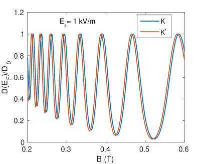
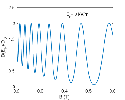
Figure 2: DOS versus magnetic field for (a) $E_{r}=1$ kV/m and (b) $E_{r}=0$ kV/m. The Fermi energy is kept at $E_{F}=0.035$ eV.

The DOS exhibits oscillation with the magnetic field-known as the SdH oscillation. The presence of an in-plane electric field is causing a valley separation in SdH oscillation too. Here, we have taken very weak brodening as $\Gamma_{0}=0.05\hbar\omega_{c}$. Here, we have computed the summation over $k_{y}$ by using the fact that the centre of the cyclotron orbit is always confined within the system i.e., $0\leq|x_{0}+G_{n}|\leq L_{x}$ or $0\leq k_{y}\leq L_{x}/l_{c}^{2}$ with $G_{n}=\lambda\sqrt{2n}l_{c}\beta_{\xi}(1-\beta_{\xi})^{-1/4}$ and sebsequently $\sum_{k_{y}}\rightarrow\frac{L_{y}}{2\pi}\int_{0}^{L_{x}/l_{c}^{2}}dk_{y}=\Omega/2\pi l_{c}^{2}$. Moreover, in the above equation, we have also ignored the $k_{y}$ dependent term ($\hbar v_{e}k_{y}$) in the LLs expression under the assumption of higher Landau level and weak electric field. As this term is not associated with valley index, hence this assumption will not affect the valley dependency of the DOS. The DOS is plotted in Fig. (2) by using Eq. (27). It is an established factZheng and Ando (2002); Raikh and Shahbazyan (1993) that the impurity induced LLs broadening in 2D Dirac material is directly proportional to $\sqrt{B}$. To plot dimensionless DOS, we consider LLs broadening width $\Gamma_{0}=0.05\hbar\omega_{c}$.

III Magnetoconductivity

In this section, we evaluate the quantum Hall conductivity and the longitudinal conductivity by using the formalism based on linear response theory developed in Ref. [Charbonneau et al., 1982] which has been extensively used in other 2D systemsPeeters and Vasilopoulos (1992); Krstajić and Vasilopoulos (2012); Shakouri et al. (2014); Tahir and Schwingenschlögl (2013, 2012); Tahir et al. (2016); Islam and Benjamin . In presence of perpendicular magnetic field, the conductivity becomes a tensor with diagonal $(\sigma_{\mu\nu}^{d})$ as well as non-diagonal $(\sigma_{\mu,\nu}^{nd})$ terms i.e., $\sigma_{\mu\nu}=\sigma_{\mu,\nu}^{d}+\sigma_{\mu,\nu}^{nd}$, where $\{\mu,\nu\}=\{x,y\}$.

III.1 Quantum Hall conductivity

The quantum Hall conductivity( $\sigma_{xy}$) of borophene can be evaluated by using the standard formula within the linear response regimeCharbonneau et al. (1982); Peeters and Vasilopoulos (1992):

$$\sigma_{xy} = \frac{ie^{2}\hbar}{\Omega}\sum_{\zeta\neq\zeta^{\prime}}f_{\zeta}(1-f_{\zeta^{\prime}}){\langle}\zeta\mid\mathcal{\hat{V}}_{x}\mid\zeta^{\prime}{\rangle}{\langle}\zeta^{\prime}\mid\mathcal{\hat{V}}_{y}\mid\zeta{\rangle}$$ (29)

$$\times \frac{1-\exp{[\beta_{T}(E_{\zeta}-E_{\zeta^{\prime}})}]}{E_{\zeta}-E_{\zeta^{\prime}}}\lim_{{\epsilon}\to 0}\frac{1}{E_{\zeta}-E_{\zeta^{\prime}}+i{\epsilon}}.$$

In the above expression, the velocity operators are defined as: $\mathcal{\hat{V}}_{x}=\partial\mathcal{H}_{0}/\partial p_{x}=\xi v_{c}\hat{\sigma}_{x}$ and $\mathcal{\hat{V}}_{y}=\partial\mathcal{H}_{0}/\partial p_{y}=v_{e}^{\xi}\mathbb{1}+\xi v_{c}\hat{\sigma}_{y}$, and $|\zeta{\rangle}\equiv|\Psi_{\zeta}(x,y){\rangle}$. Note that here we have used the transformed momentum operators i.e., $p_{x}\rightarrow(v_{x}/v_{y})^{1/2}p_{x}$ and $p_{y}\rightarrow(v_{y}/v_{x})^{1/2}p_{y}$ for the non-tilted part of the Hamiltonian. Also, $f_{\zeta}=[1+\exp\{\beta_{T}(E_{\zeta}-E_{F})\}]^{-1}$ is the Fermi-Dirac distribution function with $E_{F}$ is the Fermi energy and $\beta_{T}=(k_{B}T)^{-1}$ where $k_{B}$ is the Boltzmann constant.

By using the identity $f_{\zeta}(1-f_{\zeta^{\prime}})\{1-\exp{[\beta_{T}(E_{\zeta}-E_{\zeta^{\prime}})}]\}=f_{\zeta^{\prime}}(1-f_{\zeta})$, one can arrive at Kubo-Greenwood formula for the Hall conductivity in each valley as

$$\sigma_{xy} = \frac{ie^{2}\hbar}{\Omega}\sum_{\zeta\neq\zeta^{\prime}}(f_{\zeta}-f_{\zeta^{\prime}})\frac{{\langle}\zeta\mid\mathcal{\hat{V}}_{x}\mid\zeta^{\prime}{\rangle}{\langle}\zeta^{\prime}\mid\mathcal{\hat{V}}_{y}\mid\zeta{\rangle}}{(E_{\zeta}-E_{\zeta^{\prime}})^{2}}.$$

The velocity matrix elements in a particular valley (see Apendix A) are evaluated as (for $n>0$)

$${\langle}n,k_{y}\mid\mathcal{\hat{V}}_{x}\mid n^{\prime},k_{y}^{\prime}{\rangle}=-i\frac{v_{c}}{2\gamma_{\xi}}\big{[}\lambda\delta_{n,n^{\prime}-1}+\lambda^{\prime}\delta_{n-1,n^{\prime}}\big{]}\delta_{k_{y},{k^{\prime}}_{y}}$$ (31)

and

$${\langle}n^{\prime},k_{y}^{\prime}\mid\mathcal{\hat{V}}_{y}\mid n,k_{y}{\rangle} = -(1-\beta_{\xi}^{2})\frac{v_{c}}{2}$$ (32)

$$\times \left[\lambda^{\prime}\delta_{n^{\prime},n-1}+\lambda\delta_{n^{\prime}-1,n}\right]\delta_{k_{y},{k^{\prime}}_{y}}.$$

The presence of $\delta_{k_{y},k_{y}^{\prime}}$ guarantees that velocity matrix elements are non-zero only for $k_{y}=k_{y}^{\prime}$. To proceed further, we now follow the assumptionKrstajić and Vasilopoulos (2011) that the effects of $k_{y}$ through Fermi distribution function is very small and hence we can ignore it. This assumption is well justified for weak electric field. Moreover, it can also be seen that the $k_{y}$ dependent term inside the Fermi distribution function is independent of the Landau level index (n), for which the differences between the two Fermi distribution functions corresponding to the two successive Landau levels are almost independent of $k_{y}$. By using $\sum_{k_{y}}\rightarrow\frac{L_{y}}{2\pi}\int_{0}^{L_{x}/l_{c}^{2}}dk_{y}=\Omega/2\pi l_{c}^{2}$ in Eq. (III.1), we obtain (for $n>0$)

$$\sigma_{xy}^{\xi} = \frac{e^{2}}{h}\sum_{n}\frac{(f_{n,\xi}-f_{n+1,\xi})}{(\sqrt{2n}-\sqrt{2(n+1)})^{2}}.$$ (33)

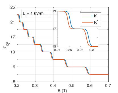
Figure 3: Quantum Hall conductivity versus magnetic field. The Hall conductivity is in units of $e^{2}/h$. The tilt velocity $v_{t}=0.32$ unit, the Fermi energy $E_{F}=0.037$ eV and the temperature is taken much low at $T=0.1$K.

At zero temperature, if $E_{F}$ lies between ${\varepsilon}_{n}$ and ${\varepsilon}_{n+1}$-th Landau level, then above expression can be reduced to

$$\sigma_{xy}^{\xi}=2\frac{e^{2}}{h}\left(n+\frac{1}{2}\right),$$ (34)

including the spin degeneracy but without valley degeneracy. The contribution which arises from $n=0$ level has to be evaluated separately. The velocity matrix elements between $n=0$ and $n^{\prime}$ are given by

$${\langle}0,k_{y}\mid\mathcal{\hat{V}}_{x}\mid n^{\prime},k_{y}^{\prime}{\rangle}=-i\frac{v_{c}}{2\gamma_{\xi}}\lambda\delta_{0,n^{\prime}-1}\delta_{k_{y},{k^{\prime}}_{y}}$$ (35)

and

$${\langle}n^{\prime},k_{y}^{\prime}\mid\mathcal{\hat{V}}_{y}\mid 0,k_{y}{\rangle} = -(1-\beta_{\xi}^{2})\frac{v_{c}}{2}\lambda\delta_{n^{\prime}-1,0}\delta_{k_{y},{k^{\prime}}_{y}}.$$ (36)

Finally, the Hall conductivity due to zero-th Landau level is

$$\sigma_{xy}^{0} = \frac{e^{2}}{h}\sum_{\xi}(f_{0,\xi}-f_{1,\xi}).$$ (37)

The quantization of Hall conductivity, in Eq. (34), is exactly similar to the case of graphene without valley degeneracy i.e,., $\sigma_{xy}=1,3,5,7,9...$ in units of $e^{2}/h$. However, the valley dependency appears at the Hall steps governed by the valley dependent Fermi-distribution function. The Hall conductivity obtained in Eq. (33) is plotted numerically in Fig. (3). The Fermi energy is taken to be $E_{F}=0.037$ eV, corresponds to carrier density $n_{e}=10^{15}m^{-2}$ and tilt velocity $v_{t}=0.32$ unit. The Fermi energy can be evaluated numerically in terms of magnetic field for a particular carrier density, as done in Ref. (Islam and Jayannavar, 2017).
The quantum Hall conductivity plots in Fig. (3) show a series of unequal quantum Hall plateaus, as expected. However, most importantly, two valleys are not following the same steps although exhibiting identical plateaus. The valley separation around the steps are exclusively caused and governed by the in-plane electric field i.e., Hall field. This feature is in complete contrast to the case of monolayer graphene under the influences of the Hall field. The origin of the valley separation at the steps can be traced to the lifting of the valley degeneracy in presence of an in-plane electric field in the Landau levels of borophene, where as in graphene such removal of valley degeneracy does not occur.

III.2 Longitudinal conductivity

In this subsection, we investigate the longitudinal conductivity. In general, the longitudinal conductivity arises mainly due to the scattering of cyclotron orbits from the charge impurities. This contribution is also known as collisional conductivity. In low temperature regime, scattering mechanism can be treated as elastic on the ground that charge carriers can not offer enough energy to excite charge impurity from its ground states to excited states during collisions. First we consider the case of the presence of a Hall field.

III.2.1 In presence of Hall field

The collisional conductivity in low temperature regime can be evaluated by using the following formulaCharbonneau et al. (1982); Peeters and Vasilopoulos (1992)

$$\sigma_{xx}=\frac{\beta_{T}e^{2}}{2\Omega}\sum_{\zeta,\zeta^{\prime}}f_{\zeta}(1-f_{\zeta^{\prime}})W_{\zeta,\zeta^{\prime}}(x_{\zeta}-x_{\zeta^{\prime}})^{2}.$$ (38)

Here, $x_{\zeta}={\langle}\zeta\mid x\mid\zeta{\rangle}$ is the average value of the x-component of the position operator of an electron in state $\mid\zeta{\rangle}$, which can be evaluated to be $x_{0}+G_{n}$ (=$k_{y}l_{c}^{2}+G_{n}$). To proceed further analytically, we can drop the $n$ dependent term ($G_{n}$) in the centre of the cyclotron orbit and thus $(x_{\zeta}-x_{\zeta^{\prime}})^{2}=(q_{y}l_{c}^{2})^{2}$ with $k_{y}^{\prime}-k_{y}=q_{y}$. Note that dropping of $G_{n}$ would not make any drastic changes in the main result except a small effect to the conductivity amplitude. Moreover, for intra Landau level scattering, $G_{n}$ would get canceled out automatically in the expression of $(x_{\zeta}-x_{\zeta^{\prime}})$. The key features of the longitudinal conductivity oscillations is preserved in the $n$-dependent part of the Landau levels in the Fermi distribution function, which controls the oscillations.

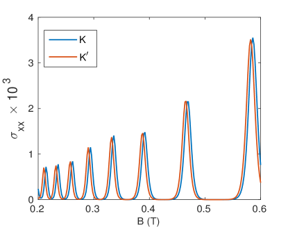
Figure 4: Longitudinal conductivity (in units of $e^{2}/h$) versus magnetic field. Other parameters are as: the Fermi energy $E_{F}=0.037$ eV, the Temperature $T=3$ K, the impurity density $n_{i}=10^{13}m^{-2}$ and LLs broadening $\Gamma_{0}=0.1\hbar\omega_{c}$.

On the other hand, the scattering rate between states $|\zeta{\rangle}$ and $|\zeta^{\prime}{\rangle}$ is given by

$$W_{\zeta,\zeta^{\prime}}=\frac{2\pi n_{i}}{\Omega\hbar}\sum_{q}\mid U_{q}\mid^{2}\mid F_{\zeta,\zeta^{\prime}}(\eta)\mid^{2}\delta(E_{\zeta}-E_{\zeta^{\prime}})\delta_{k_{y},k_{y}^{\prime}+q_{y}}.$$ (39)

Here, $n_{i}$ is the impurity density and $\eta=q^{2}l_{c}^{2}/2$. The $2$D Fourier transformation of the screened charged impurity potential $U(r)=[e^{2}/{4\pi\epsilon_{0}\epsilon_{r}r}]e^{-k_{s}r}$ is $U_{q}=U_{0}[q^{2}+k_{s}^{2}]^{-1/2}\simeq U_{0}/k_{s}$ for short range delta function-like potential, where $U_{0}=e^{2}/(2\epsilon_{0}\epsilon_{r})$ and $k_{s}$ is the screening vector. The form factor is defined as $F_{\zeta,\zeta^{\prime}}(\eta)={\langle}\zeta\mid e^{i\vec{q}.\vec{r}}\mid\zeta^{\prime}{\rangle}$, which can be evaluated (See Apendix B) considering only $n^{\prime}=n\pm 1$ (because of the presence of $\delta_{k_{y},k_{y^{\prime}}+q_{y}}$ in $W_{\zeta,\zeta^{\prime}}$)

$$\mid F_{n,n\pm 1}(\eta)\mid^{2}=e^{-\eta}[R_{n,n\pm 1}(\eta)]^{2}$$ (40)

with

$$R_{n,n+1}(\eta)\simeq\frac{1}{\sqrt{2(n+1)}}L_{n}^{1}(\eta)+\frac{1}{\sqrt{2n}}L_{n-1}^{1}(\eta)$$ (41)

and

$$R_{n,n-1}(\eta)\simeq\sqrt{\frac{2}{n}}L_{n-1}^{1}(\eta)+\sqrt{\frac{2}{n-1}}L_{n-2}^{1}(\eta).$$ (42)

Here, $L_{n}(\eta)$ is the Laguerre polynomial of order $n$. For lowest LL ($n=0$), the scattering amplitude has to be evaluated separately as

$$\mid F_{0,1}(\eta)\mid^{2}=e^{-\eta}\frac{1}{2}[L_{0}^{1}(\eta)]^{2}.$$ (43)

By replacing summation over $k_{y}$ by $\Omega/(2\pi l_{c}^{2})$, $\sum_{q}\rightarrow\frac{\Omega}{(2\pi)^{2}}\int qdqd\phi$ and $(x_{\xi}-x_{\xi^{\prime}})^{2}=q_{y}^{2}l_{c}^{4}=(q\sin\phi)^{2}l_{c}^{4}$ , the Eq. (38) can be further simplified to $\sigma_{xx}=\sum_{\xi}\sigma^{\xi}$ with

$$\sigma_{xx}^{\xi}\simeq\frac{e^{2}}{h}\frac{n_{i}U_{s}^{2}}{2\pi l_{c}^{2}\Gamma_{0}}\beta_{T}\sum_{n,\xi}I_{n}f_{n,\xi}(1-f_{n,\xi}).$$ (44)

Here, $U_{s}=U_{0}/k_{s}$, $\Gamma_{0}$ is the impurity induced LLs broadening and

$$I_{n}=\int_{0}^{\infty}\eta^{2}e^{-\eta}\left([R_{n,n+1}(\eta)]^{2}+[R_{n,n-1}(\eta)]^{2}\right)d\eta.$$ (45)

The cut-off limit of the above integration can be extracted from the short range scattering condition i.e., $q<<k_{s}$ ($\eta<<\eta_{s}$ with $\eta_{s}=k_{s}^{2}l_{c}^{2}/2$).

We plot longitudinal conductivity in Fig. (4) by using Eq. (44). For this numerical plot, we use the following parameters: charge density $n_{e}=10^{15}m^{-2}$, impurity density $n_{i}=10^{13}m^{-2}$, temperature $T=3$ K, dielectric constant of borophene is taken to be $\kappa=10$ which is in consistent with Ref. [Sadhukhan and Agarwal, 2017] and screening vector $k_{s}=10^{8}m^{-1}$. We also consider the magnetic field dependency of the impurity induced LLs broadening as $\Gamma_{0}\simeq 0.1\hbar\omega_{c}$. As it is proven factPeeters and Vasilopoulos (1992); Nasir et al. (2010) that SdH oscillation start to die out with the increasing temperature, hence we give plots only for a particular temperature.

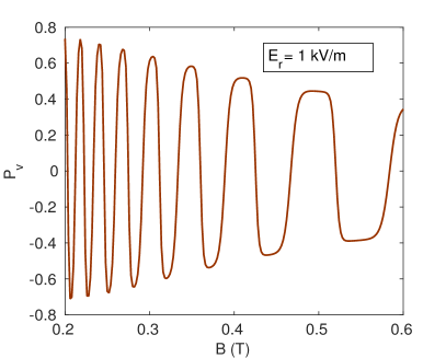
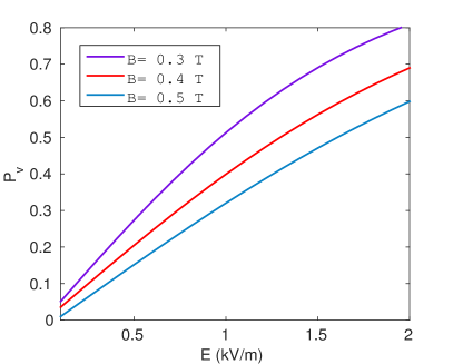
Figure 5: Polarization in the longitudinal conductivity versus (a) magnetic field and (b) electric field.

The longitudinal conductivity peaks are corresponding to the crossing of Fermi level through the LLs. However, because of the valley separation in LLs, conductivity peaks in two valleys are not at the same location. The separation of the conductivity peaks in two valleys are the direct consequences of the lifting of the valley degeneracy in the LLs. The gap between two consecutive peaks in each valley increases with the increase of magnetic field and this is obvious as the LLs spacing between two successive LLs also increases with the magnetic field.

In Fig. (5)a, we plot the polarization in the longitudinal conductivity versus magnetic field and electric field by using the relation

$$P_{\rm v}=\frac{\sigma_{xx}^{+}-\sigma_{xx}^{-}}{\sigma_{xx}^{+}+\sigma_{xx}^{-}}.$$ (46)

It shows that a sizable valley polarization can be achieved for a wide range of magnetic field by applying a Hall field. However, the polarization appears to be oscillatory with magnetic field. This is because of the oscillatory nature of longitudinal conductivity with magnetic field in both valleys. On the other hand, we also show the evolution of polarization with electric field for three values of magnetic field in Fig. (5)b which shows that a sizable polarization can emerge for an electric field $E>0.5$ kV/m. Note that although a weak fluctuation of Fermi energy between nearest LLs does exist with respect to the magnetic field [see Ref. (Islam and Jayannavar, 2017)], we keep Fermi level constant in the regime of interest as the amplitude of Fermi energy fluctuation is very small.

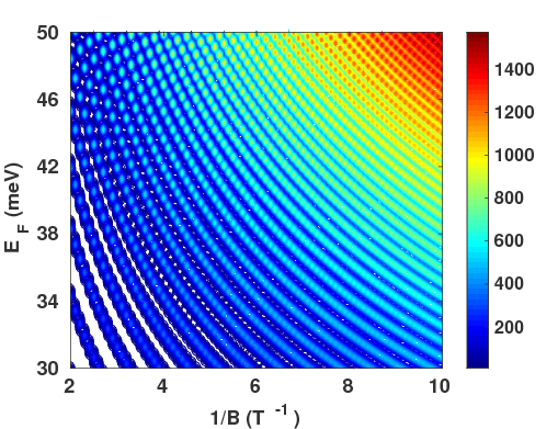
Figure 6: (Color online) Contour plot of longitudinal conductivity (in units of $e^{2}/h$) in the plane of $1/B$ and $E_{F}$. The temperature is taken as $T=3$ K.

III.2.2 In absence of Hall field

In this subsection, we evaluate the longitudinal conductivity in absence of the Hall field. In absence of the Hall field ($E_{r}=0$), the LLs regain the valley degeneracy and hence the valley dependent transport is not expected anymore. The scenario is now quite similar to the case of the monolayer graphene without Hall field, except the renormalized Fermi velocity $v_{c}=\sqrt{v_{x}v_{y}}$ and tilting of the Dirac cones. Moreover, in absence of the Hall field the LLs not only recover the valley degeneracy but also get back the $k_{y}$ degeneracy for which the intra-LLs scattering is now allowed, and the scattering rate between states $|\zeta{\rangle}$ and $|\zeta^{\prime}{\rangle}$ is now given by

$$W_{\zeta,\zeta^{\prime}}=\frac{2\pi n_{i}}{\Omega\hbar}\sum_{q}\mid U_{q}\mid^{2}\mid Q_{\zeta,\zeta^{\prime}}(\eta)\mid^{2}\delta(E_{\zeta}-E_{\zeta^{\prime}})\delta_{k_{y},k_{y}^{\prime}+q_{y}}.$$ (47)

Here,

$$\mid Q_{n,n}(\eta)\mid^{2}=\frac{e^{-\eta}}{4}[J_{n,n}(\eta)+J_{n-1,n-1}(\eta)]^{2}$$ (48)

Following the Ref. [Krstajić and Vasilopoulos, 2012; Nasir et al., 2010], we obtain the longitudinal conductivity as

$$\sigma_{xx}\simeq\frac{e^{2}}{h}\frac{n_{i}U_{s}^{2}}{\pi l_{c}^{2}\Gamma_{0}}\beta_{T}\sum_{n}nf_{n}(1-f_{n})$$ (49)

which is plotted in Fig. 6 in the plane of Fermi level and inverse magnetic field. The longitudinal conductivity shows SdH oscillations with inverse magnetic field as well as Fermi level both with different frequencies. The conductivity amplitude increases with the Fermi level as well as inverse magnetic field. However, to understand the effect of tilt parameter on SdH oscillations frequency, we plot the longitudinal conductivity versus inverse magnetic field for both cases i.e., in absence and presence of tilt parameter in Fig. 7.

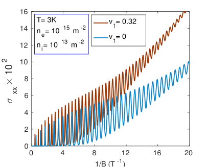
Figure 7: (Color online) Longitudinal conductivity (in units of $e^{2}/h$) versus inverse magnetic field. The Fermi level $E_{F}=0.037$ eV.

It is observed that the frequency as well as the amplitude of the longitudinal conductivity are significantly affected by the tilt parameter. To get a clear picture of the influences of the tilt parameter on the SdH oscillations, an approximate analytical simplification of the longitudinal conductivity is necessary. To obtain analytical expression of Eq. (49), we replace the summation over LL index $n$ as: $\sum_{n}\rightarrow\pi l_{c}^{2}\int_{0}^{\infty}D(E)dE$, where $D(E)$ is the density of states (DOS). The analytical approximate form of the DOS can be obtained by following the Refs.[Peeters et al., ; Tsaran and Sharapov, 2014; Islam and Ghosh, ] as

$$D(E)\simeq\frac{2E}{\pi(\hbar v_{c})^{2}}\left\{1+2\Omega(E)\cos\left[2\pi\left(\frac{E}{\hbar\bar{\omega}_{c}}\right)^{2}\right]\right\},$$ (50)

where impurity induced damping factor is $\Omega(E)=\exp\left\{-2\pi\left[\frac{\Gamma(E)E}{(\hbar\bar{\omega}_{c})^{2}}\right]\right\}$ with $\Gamma(E)=4\pi\Gamma_{0}^{2}E/(\hbar\bar{\omega}_{c})^{2}$ and $\bar{\omega}_{c}=\omega_{c}/(1-\beta^{2})^{3/4}$ with $\beta=v_{t}/v_{c}$. Using the above form of DOS in Eq. (49), one can readily find

$$\sigma_{xx}\simeq\frac{e^{2}}{h}U\left\{1+2\Omega(E_{F})\frac{T/T_{c}}{\sinh(T/T_{c})}\cos\left[2\pi\left(\frac{f}{B}\right)\right]\right\}.$$ (51)

Here, $U$ is a dimensionless factor and given by

$$U=\frac{n_{i}U_{s}^{2}}{2\Gamma_{0}}\left[\frac{E_{F}}{\hbar\bar{\omega}_{c}}\right]^{2}\frac{E_{F}}{\pi(\hbar v_{c})^{2}}.$$ (52)

On the other hand, the SdH oscillations frequency with the inverse magnetic field is given by

$$f=\frac{1}{e\hbar}\left(\frac{E_{F}}{v_{c}}\right)^{2}g_{t},$$ (53)

where $g_{t}=1/(1-\beta^{2})^{3/2}>1$. The above expression shows that the tilt parameter amplifies the frequency of the SdH oscillation by a factor $g_{t}=1.1526$. The characteristic temperature is defined by $k_{B}T_{c}=(\hbar\bar{\omega}_{c})^{2}/(4\pi^{2}E_{F})$, beyond which the SdH oscillation start to die out. Note that apart from the frequency, the characteristic temperature is also affected by the tilt parameter.

In addition to the inverse magnetic field, longitudinal conductivity also exhibits similar SdH oscillation with the Fermi energy. The SdH oscillations frequency with Fermi energy is

$$\bar{f}=\frac{E_{F}}{(\hbar\omega_{c})^{2}}g_{t}.$$ (54)

This expression shows that unlike the frequency of SdH oscillations with inverse magnetic field [see Eq. (53)], SdH oscillations with the Fermi energy is non-periodic as the frequency itself depends on the Fermi level strongly. The tilted parameter suppresses SdH oscillation frequency in both cases in similar fashion. The longitudinal conductivity shows the SdH oscillations with the inverse magnetic field and the Fermi energy both.

IV Effects of strain

In this section, we investigate how the application of strain can influence the magnetoconductiity in absence and presence of an in-plane electric field. The issue of strain induced valley polarization in Dirac material is not new rather it has been extensively considered in graphenePereira and Castro Neto (2009b); Pereira et al. (2009); Roy et al. (2013) to siliceneLi et al. (2018); Farokhnezhad et al. (2017). In Ref. [Zabolotskiy and Lozovik, 2016], strain induced quantum valley Hall effect was also predicted. However, in this work, we would like to consider the case of interplay between the in-plane electric field and the strain. The strain can be described by the displacement field $\mathcal{U}(r)$ and the strain tensor $\mathcal{U}_{ij}=\frac{1}{2}[(\frac{\partial\mathcal{U}_{i}}{\partial r_{j}})+(\frac{\partial\mathcal{U}_{j}}{\partial r_{i}})]$. The strained borophene must not violate any symmetry possessed by the material. Similar to the graphene, the strain acts as a pseudo magnetic field. However, the strain induced vector potential in two valleys are in opposite sign and it can be captured in low energy effective Hamiltonian in presence of a real magnetic field (B) as

$$H=\xi[v_{x}p_{x}\sigma_{x}+v_{y}(p_{y}+eA_{S})\sigma_{y}+v_{t}(p_{y}+eA_{S})\mathbb{1}].$$ (55)

Here, the vector potential $A_{S}=x(B+\xi t)$ with the strain induced pseudo magnetic field $t=[(\frac{\partial{A}_{y}}{\partial x})-(\frac{\partial{A}_{x}}{\partial y})]$. Here, the different components of vector potential can be expressedZabolotskiy and Lozovik (2016) as ${\bf A}=[\alpha_{xy}\mathcal{U}_{xy},\alpha_{xx}\mathcal{U}_{xx}+\alpha_{yy}\mathcal{U}_{yy}$] with $\alpha_{xy}=3.86$ G-cm, $\alpha_{xx}=3.58$ G-cm and $\alpha_{yy}=-1.15$ G-cm. The strain field in 8-Pmmn borophene is taken to be as $\mathcal{U}(r)=(0,x^{2}/L,0)$. The strain induced magnetic field can be estimated to be around $t=100$ T for the sample length of $10$ nm. This is in fact an advantage of strain that one can generate very large magnetic field. However, in our case we shall keep the strain induced magnetic field much smaller in order to compete it with the real magnetic field. The Landau levels of strained borophene in absence of the in-plane electric field can be obtained following the Sec.(II). as

$$E_{\zeta}=\lambda\hbar\omega_{\xi}\sqrt{2n}(1-\beta^{2})^{3/4},$$ (56)

where $\omega_{\xi}=\sqrt{v_{x}v_{y}}/l_{\xi}$ with $l_{\xi}=\sqrt{\hbar/e(B+\xi t)}$. The Landau levels of strained borophene is sensitive to the valley index, which is in fact similar to the case of graphene. On the other hand if we switch-on the in-plane electric field the Landau levels becomes

$$E_{\zeta}=\lambda\hbar\omega_{\xi}\sqrt{2n}(1-\beta_{\xi}^{2})^{3/4}-\hbar k_{y}\left[\frac{E_{r}}{B+\xi t}\right],$$ (57)

where the valley dependency is now attributed to two different origin. One is the valley dependent cyclotron frequency arises from the effect of strain and other one is the in plane electric field induced valley dependency of $\beta_{\xi}=[E_{r}/(B+\xi t)+\xi v_{t}]/\sqrt{v_{x}v_{y}}$. The critical electric field, needed for LLs in each valley to get collapsed, in presence of strain would be also modified as $E_{r}=(B+\xi t)(v_{c}+\xi v_{t})$. The quantum Hall conductivity corresponding to each valley are plotted in Fig. (8) for different combination of strain and electric field. In Fig. (8)a, we show that both valley are showing identical plateaus as expected in absence of any in-plane electric field and strain. The effect of electric field is shown again here in Fig. (8)b, showing small separation between two valleys in its steps. The inclusion of strain is plotted in Fig. (8)c, which shows that the valley separation is very large and dominated by the effect of the valley dependent cyclotron frequency in LLs. Finally, we show only the effect of strain without any in-plane electric field in Fig. (8)d which is very similar to Fig. (8)c confirming the fact that strain alone can dominate the valley polarization even in presence of a Hall field.

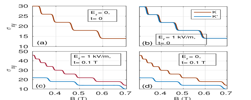
Figure 8: (Color online) Plots of quantum Hall conductivity (in units of $e^{2}/h$) versus magnetic field. The temperature is taken as $T=2$ K.

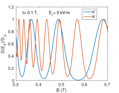
Figure 9: Density of states iin presence of strain versus real magnetic field. The tilt velocity $v_{t}=0.32$ unit and the Fermi energy $E_{F}=0.037$ eV.

Finally, we shall discuss the case of an in-plane electric field and strain without any real magnetic field. From the above discussion, we can write the Landau levels in absence of the real magnetic field but in presence of the pseudo magnetic field (strain) by just setting $B=0$ in Eq. (58). However, the LLs in presence of pseudo magnetic field and a in-plane electric field will be identical to Eq. (58) except the tilt dependent factor $\beta_{\xi}=\xi\beta$ with $\beta=(E_{r}/t+v_{t})/\sqrt{v_{x}v_{y}}$ leading to the LLs as

$$E_{\zeta}=\lambda\hbar\omega\sqrt{2n}(1-\beta^{2})^{3/4}-\xi\hbar k_{y}\left(\frac{E_{r}}{t}\right).$$ (58)

Here, the valley index is not intrinsically associated with the LLs index $n$, for which valley dependent magnetotransport is not expected under our assumption of weak electric field. Hence, we can conclude that the in-plane electric field looses its ability to produce valley dependent Hall steps in quantum Hall conductivity if real magnetic field is replaced by strain induced pseudo magnetic field.

The difference in the size of plateaus in presence of strain, as shown in Fig. (8)d, can also be explained from the SdH oscillation feature in DOS plots in Fig. (9). Here, both valley exhibit large frequency differences in SdH oscillation, which reflects as unequal plateaus in Hall conductivity too.

V Summary and conclusions

In this work, we have studied the magnetotransport properties of a 2D sheet of the polymorph of $8$-$Pmmn$ borophene which exhibits tilted anisotropic Dirac cones in its band structure. We have applied an in-plane electric field (Hall field) to remove the valley degeneracy in its LLs. The signatures of the lifting of the valley degeneracy in the LLs are examined in the magnetotransport properties. We have evaluated the quantum Hall and the longitudinal conductivity in presence of the Hall field by using linear response theory. The presence of the Hall field causes valley dependent longitudinal and Hall conductivity, which is in complete contrast to the case of monolayer grapheneKrstajić and Vasilopoulos (2011) where the Hall field does not remove the valley degeneracy from its LLs. A sizable valley polarization can be achieved in the longitudinal conductivity by applying a Hall field which can be linked to the field of valleytronics where valley dependent transport by tuning external parameter is one of the the key requirement. Here, it is worthwhile to mention that the external in-plane electric field should be along the direction of tilt induced pseudo electric field. If external real electric field is taken perpendicular to the direction of pseudo electric field then exact solution is not possible and numerical study may not yield valley polarization as the real electric field will affect almost equally to both valleys.

Moreover, we have also noted by analyzing analytical results that SdH oscillation frequency is enhanced by the tilting of the Dirac cones. Finally we have also discussed the possible scenario if the real magnetic field is replaced by a strain induced pseudo magnetic field and found that in this case Hall field can not lift the valley degeneracy. However, if the real and pseudo magnetic field both present then the lifting of the valley degeneracy would be dominated by the strain induced pseudo magnetic field.

Appendix A

The velocity matrix elements are given by

$${\langle}n,k_{y}|\hat{\mathcal{V}}_{x}|n^{\prime},k^{\prime}_{y}{\rangle}=\xi v_{c}{\langle}n|\hat{\sigma}_{x}|n^{\prime}{\rangle}\delta_{k_{y},k_{y}^{\prime}}$$

$$=\xi\frac{v_{c}}{2\gamma_{\xi}}(\lambda^{\prime}A^{\dagger}\phi_{n}+i\xi B^{\dagger}\phi_{n-1})\sigma_{x}(\lambda A\phi_{n^{\prime}}+i\xi B\phi_{n^{\prime}-1})$$

where

$$A=\left(\begin{array}[c]{c}\cosh(\theta_{\xi}/2)\\ -i\sinh(\theta_{\xi}/2)\end{array}\right)$$ (59)

and

$$B=\left(\begin{array}[c]{c}i\sinh(\theta_{\xi}/2)\\ \cosh(\theta_{\xi}/2)\end{array}\right)$$ (60)

abd subsequently the above Eq. (A) can be easily reduced to

$${\langle}n,k_{y}|\hat{\mathcal{V}}_{x}|n^{\prime},k^{\prime}_{y}{\rangle}$$

$$=-i\frac{v_{c}}{2\gamma_{\xi}}[\lambda\delta_{n-1,n^{\prime}}+\lambda^{\prime}\delta_{n,n^{\prime}-1}]\delta_{k_{y},k_{y}^{\prime}}.$$ (61)

Similarly, the another matrix elements

$${\langle}n^{\prime},k^{\prime}_{y}|\hat{\mathcal{V}}_{y}|n,k_{y}{\rangle}={\langle}n^{\prime}|v_{e}^{\xi}\mathbb{1}+\xi v_{c}\hat{\sigma}_{y}|n{\rangle}\delta_{k_{y},k_{y}^{\prime}}$$ (62)

$$= -\frac{1}{2\gamma_{\xi}}[v_{c}\cosh(\theta_{\xi})-v_{e}^{\xi}\sinh(\theta_{\xi})]$$

$$\times [\lambda^{\prime}\delta_{n^{\prime},n-1}+\lambda\delta_{n^{\prime}-1,n}]$$

Now, we shall use the relation $\cosh(\theta_{\xi})=\gamma_{\xi}$ and $\sinh(\theta_{\xi})=\beta_{\xi}\gamma_{\xi}$ to obtain

$${\langle}n^{\prime},k^{\prime}_{y}|\hat{\mathcal{V}}_{y}|n,k_{y}{\rangle} = -\frac{v_{c}}{2}(1-\beta_{\xi}^{2})$$ (63)

$$[\lambda^{\prime}\delta_{n^{\prime},n-1}+\lambda\delta_{n^{\prime}-1,n}]\delta_{k_{y},k_{y}^{\prime}}.$$

Appendix B

To calculate the scattering rate between two states, the scattering matrix can be expressed as

$$F_{\zeta,\zeta^{\prime}} = {\langle}\zeta|e^{i{\bf q.r}}|\zeta^{\prime}{\rangle}={\langle}n,k_{y}|e^{i{\bf q.r}}|n^{\prime},k^{\prime}_{y}{\rangle}$$ (64)

$$\simeq e^{-\eta/2}R_{n,n^{\prime}}(\eta)\delta_{k^{\prime}_{y},k_{y}-q_{y}}e^{-i\Theta-\frac{\eta}{2}}$$

with $\Theta=l_{c}q_{x}(-k_{y}+q_{y}/2)$. Here, we have also used the following standard integral results as: for $n^{\prime}\geq n$

$$R_{n,n^{\prime}}=\left[\frac{2^{n}n!}{2^{n^{\prime}}n^{\prime}!}\right]^{1/2}\upsilon^{n^{\prime}-n}L_{n}^{n^{\prime}-n}(\eta)e^{-\eta/2}$$ (65)

and for $n^{\prime}\leq n$

$$R_{n,n^{\prime}}=\left[\frac{2^{n}n^{\prime}!}{2^{n^{\prime}}n!}\right]^{1/2}(-\upsilon^{*})^{n-n^{\prime}}L_{n^{\prime}}^{n-n}(\eta)e^{-\eta/2},$$ (66)

where $\upsilon=l_{c}(q_{x}+iq_{y})/2$ and $L_{n}^{n^{\prime}}(\eta)$ is the Laguerre polymonial. More details about these matrix elements evaluation can be found in Refs. [Krstajić and Vasilopoulos, 2011; Peeters and Vasilopoulos, 1992].