Summary

Large scale neural recordings have established that the transformation of sensory stimuli into motor outputs relies on low-dimensional dynamics at the population level, while individual neurons exhibit complex selectivity. Understanding how low-dimensional computations on mixed, distributed representations emerge from the structure of the recurrent connectivity and inputs to cortical networks is a major challenge. Here, we study a class of recurrent network models in which the connectivity is a sum of a random part and a minimal, low-dimensional structure. We show that, in such networks, the dynamics are low dimensional and can be directly inferred from connectivity using a geometrical approach. We exploit this understanding to determine minimal connectivity required to implement specific computations, and find that the dynamical range and computational capacity quickly increase with the dimensionality of the connectivity structure. This framework produces testable experimental predictions for the relationship between connectivity, low-dimensional dynamics and computational features of recorded neurons.

Introduction

Understanding the relationship between synaptic connectivity, neural activity and behavior is a central endeavor of neuroscience. Networks of neurons encode incoming stimuli in terms of electrical activity and transform this information into decisions and motor actions through synaptic interactions, thus implementing computations that underly behavior. Reaching a simple, mechanistic grasp of the relation between connectivity, activity and behavior is, however, highly challenging. Cortical networks, which are believed to constitute the fundamental computational units in the mammalian brain, consist of thousands of neurons that are highly inter-connected through recurrent synapses. Even if one were able to experimentally record the activity of every neuron and the strength of each synapse in a behaving animal, understanding the causal relationships between these quantities would remain a daunting challenge because an appropriate conceptual framework is currently lacking (Gao and Ganguli, 2015). Simplified, computational models of neural networks provide a testbed for developing such a framework. In computational models and trained artificial neural networks, the strengths of all synapses and the activity of all neurons are known, yet an understanding of the relation between connectivity, dynamics and input-output computations has been achieved only in very specific cases (e.g. Hopfield (1982); Ben-Yishai et al. (1995); Wang (2002)).

One of the most popular and best-studied classes of network models is based on fully random recurrent connectivity (Sompolinsky et al., 1988; Brunel, 2000; van Vreeswijk and Sompolinsky, 1996). Such networks display internally generated irregular activity that closely resembles spontaneous cortical patterns recorded in-vivo (Shadlen and Newsome, 1998). However, randomly connected recurrent networks display only very stereotyped responses to external inputs (Rajan et al., 2010), can implement only a limited range of input-output computations and their spontaneous dynamics are typically high dimensional (Williamson et al., 2016). To implement more elaborate computations and low-dimensional dynamics, classical network models rely instead on highly structured connectivity, in which every neuron belongs to a distinct cluster, and is selective to only one feature of the task (e.g. Wang (2002); Amit and Brunel (1997); Litwin-Kumar and Doiron (2012)). Actual cortical connectivity appears to be neither fully random nor fully structured (Harris and Mrsic-Flogel, 2013), and the activity of individual neurons displays a similar mixture of stereotypy and disorder (Rigotti et al., 2013; Mante et al., 2013; Churchland and Shenoy, 2007). To take these observations into account and implement general-purpose computations, a large variety of functional approaches have been developed for training recurrent networks and designing appropriate connectivity matrices (Hopfield, 1982; Jaeger and Haas, 2004; Maass et al., 2007; Sussillo and Abbott, 2009; Eliasmith and Anderson, 2004; Boerlin et al., 2013; Pascanu et al., 2013; Martens and Sutskever, 2011). A unified conceptual picture of how connectivity determines dynamics and computations is, however, currently missing (Barak, 2017; Sussillo, 2014).

Remarkably, albeit developed independently and motivated by different goals, several of the functional approaches for designing connectivity appear to have reached similar solutions (Hopfield, 1982; Jaeger and Haas, 2004; Sussillo and Abbott, 2009; Eliasmith and Anderson, 2004; Boerlin et al., 2013), in which the implemented computations do not determine every single entry in the connectivity matrix but instead rely on a specific type of minimal, low-dimensional structure, so that in mathematical terms the obtained connectivity matrices are low rank. In classical Hopfield networks (Hopfield, 1982; Amit et al., 1985), a rank-one term is added to the connectivity matrix for every item to be memorized, and each of these terms fixes a single dimension, i.e. row/column combination, of the connectivity matrix. In echo-state (Jaeger and Haas, 2004; Maass et al., 2007) and FORCE learning (Sussillo and Abbott, 2009), and similarly within the Neural Engineering Framework (Eliasmith and Anderson, 2004), computations are implemented through feedback loops from readout units to the bulk of the network. Each feedback loop is mathematically equivalent to adding a rank-one component and fixing a single row/column combination of the otherwise random connectivity matrix. In the predictive spiking theory (Boerlin et al., 2013) the requirement that information is represented efficiently leads again to a connectivity matrix with similar low-rank form. Taken together, the results of these studies suggest that a minimal, low-rank structure added on top of random recurrent connectivity may provide a general and unifying framework for implementing computations in recurrent networks.

Based on this observation, here we study a class of recurrent networks in which the connectivity is a sum of a structured, low-rank part and a random part. We show that in such networks, both spontaneous and stimulus-evoked activity are low-dimensional and can be predicted from the geometrical relationship between a small number of high-dimensional vectors that represent the connectivity structure and the feed-forward inputs. This understanding of the relationship between connectivity and network dynamics allows us to directly design minimal, low-rank connectivity structures that implement specific computations. We focus on four tasks of increasing complexity, starting with basic binary discrimination and ending with context-dependent evidence integration (Mante et al., 2013). We find that the dynamical repertoire of the network increases quickly with the dimensionality of the connectivity structure, so that rank-two connectivity structures are already sufficient to implement complex, context-dependent tasks (Mante et al., 2013; Saez et al., 2015). For each task, we illustrate the relationship between connectivity, low-dimensional dynamics and the performed computation. In particular, our framework naturally captures the ubiquitous observation that single-neuron responses are highly heterogeneous and mixed (Rigotti et al., 2013; Mante et al., 2013; Churchland and Shenoy, 2007; Machens et al., 2010), while the dimensionality of the dynamics underlying computations is low and increases with task complexity (Gao and Ganguli, 2015). Crucially, for each task, our framework produces experimentally testable predictions that directly relate connectivity, the dominant dimensions of the dynamics, and the computational features of individual neurons.

Results

We studied a class of models which we call low-rank recurrent networks. In these networks, the connectivity matrix was given by a sum of an uncontrolled, random matrix and a structured, controlled matrix $P$. The structured matrix $P$ was low rank, i.e. it consisted only of a small number of independent rows and columns, and its entries were assumed to be weak (of order $1/N$, where $N$ is the number of units in the network). We considered $P$ moreover to be fixed and known, and uncorrelated with the random part $g\chi$, which was considered unknown except for its statistics (mean 0, variance ${g^{2}}/{N}$). As in classical models, the networks consisted of $N$ firing rate units with a sigmoid input-output transfer function (Sompolinsky et al., 1988; Sussillo and Abbott, 2009):

$$\dot{x}_{i}(t)=-x_{i}(t)+\sum_{j=1}^{N}J_{ij}\phi(x_{j}(t))+I_{i},$$ (1)

where $x_{i}(t)$ is the total input current to unit $i$, $J_{ij}=g\chi_{ij}+P_{ij}$ is the connectivity matrix, $\phi(x)=\tanh(x)$ is the current-to-rate transfer function, and $I_{i}$ is the external, feed-forward input to unit $i$.

To connect with the previous literature and introduce the methods that underlie our results, we start by describing the spontaneous dynamics ($I_{i}=0$) in a network with a unit-rank structure $P$. We then turn to the response to external inputs, the core of our results that we exploit to demonstrate how low-rank networks can implement four tasks of increasing complexity.

One-dimensional spontaneous activity in networks with unit-rank structure

We started with the simplest possible type of low-dimensional connectivity, a matrix $P$ with unit-rank (Fig. 1 A). Such a matrix is specified by two $N$-dimensional vectors $m=\{m_{i}\}$ and $n=\{n_{j}\}$, which fully determine all its entries. Every column in this matrix is a multiple of the vector $m$, and every row is a multiple of the vector $n$, so that the individual entries are given by

$$P_{ij}=\frac{m_{i}n_{j}}{N}.$$ (2)

We will call $m$ and $n$ respectively the right- and left-connectivity vectors (as they correspond to the right and left eigenvectors of the matrix $P$, see Methods), and we consider them arbitrary, but fixed and uncorrelated with the random part of the connectivity. As we will show, the spontaneous network dynamics can be directly understood from the geometrical arrangement of the vectors $m$ and $n$.

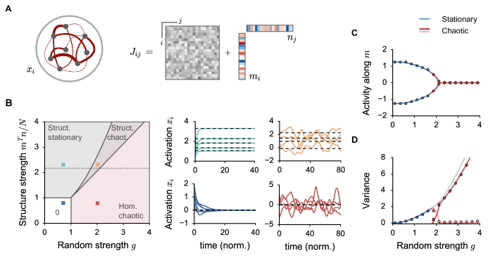
Figure 1: Spontaneous activity in random networks with unit-rank connectivity structure. A. The recurrent network model, whose connectivity matrix consists of the sum of a random (gray) and of a structured unit-rank (colored) component. B. Left: dynamical regimes of the network activity as function of the structure connectivity strength $m^{T}n/N$ and the random strength $g$. Gray areas: bistable activity; red: chaotic activity. Side panels: samples of dynamics from finite networks simulations (parameters indicated by colored dots in the phase diagram). C-D. Activity statistics as the random strength $g$ is increased and the structure strength is fixed to $2.2$ (dashed line in B). C: Activity along the vector $m$, as quantified by $\kappa=\langle n_{i}[\phi_{i}]\rangle$. Blue (resp. red) lines: theoretical prediction for stationary (resp. chaotic) dynamics. D: Activity variance due to random connectivity. Blue and pink lines: static heterogeneity, red: temporal variance that quantifies chaotic activity. Dots: simulations of finite-size networks. See Methods for details.

In absence of structured connectivity, the dynamics are determined by the strength $g$ of the random connectivity: for $g<1$, the activity in absence of inputs decays to zero, while for $g>1$ it displays strong, chaotic fluctuations (Sompolinsky et al., 1988). Our first aim was to understand how the interplay between the fixed, low-rank part and the random part of the connectivity shapes the spontaneous activity in the network.

Our analysis of network dynamics relies on an effective, statistical description that can be mathematically derived if the network is large and the low-dimensional part of the connectivity is weak (i.e. if $P_{ij}$ scales inversely with the number of units $N$ in the network as in Eq. 2). Under those assumptions, the activity of each unit can be described in terms of the mean and variance of the total input it receives. Dynamical equations for these quantities can be derived by extending the classical dynamical mean-field theory (Sompolinsky et al., 1988). This theory effectively leads to a low-dimensional description of network dynamics in terms of equations for a couple of macroscopic quantities. Full details of the analysis are provided in the Methods; here, we focus only on the main results.

The central ingredient of the theory is an equation for the average equilibrium input $\mu_{i}$ to unit $i$:

$$\mu_{i}=\kappa m_{i},\quad\mathrm{where}\quad\kappa=\frac{1}{N}\sum_{j=1}^{N}n_{j}\big{[}\phi_{j}\big{]}.$$ (3)

The scalar quantity $\kappa$ represents the overlap between the left-connectivity vector $n$ and the $N$-dimensional vector $[\phi]=\{\big{[}\phi_{j}\big{]}\}$ that describes the mean firing activity of the network ($[\phi_{j}]$ is the firing rate of unit $j$ averaged over different realizations of the random component of the connectivity, and depends implicitly on $\kappa$). The overlap $\kappa$ therefore quantifies the degree of structure along the vector $n$ in the activity of the network. If $\kappa>0$, the equilibrium activity of each neuron is correlated with the corresponding component of the vector $n$, while $\kappa=0$ implies no such structure is present. The overlap $\kappa$ is the key macroscopic quantity describing the network dynamics, and our theory provides equations specifying its dependence on network parameters.

If one represents the network activity as a point in the $N-$dimensional state-space where every dimension corresponds to the activity of a single unit, Eq. 3 shows that the structured part of the connectivity induces a one-dimensional organization of the spontaneous activity along the vector $m$. This one-dimensional organization, however, emerges only if the overlap $\kappa$ does not vanish. As the activity of the network is organized along the vector $m$, and $\kappa$ quantifies the projection of the activity onto the vector $n$, non-vanishing values of $\kappa$ require a non-vanishing overlap between vectors $m$ and $n$. This overlap, given by $m^{T}n/N=\sum_{j}m_{j}n_{j}/N$, directly quantifies the strength of the structure in the connectivity. The connectivity structure strength $m^{T}n/N$ and the activity structure strength $\kappa$ are therefore directly related, but in a highly non-linear manner. If the connectivity structure is weak, the network only exhibits homogeneous, unstructured activity corresponding to $\kappa=0$ (Fig. 1 B blue). If the connectivity structure is strong, structured heterogeneous activity emerges ($\kappa>0$), and the activity of the network at equilibrium is organized in one dimension along the vector $m$ (Fig. 1 B green and C), while the random connectivity induces additional heterogeneity along the remaining $N-1$ directions. Note that, because of the symmetry in the specific input-output function we use, when a heterogeneous equilibrium state exists, the configuration with the opposite sign is an equilibrium state too, so that the network activity is bistable (for more general asymmetric transfer functions, this bistability is still present, although the symmetry is lost, see Fig. S7).

The random part of the connectivity disrupts the organization of the activity induced by the connectivity structure through two different effects. The first effect is that as the random strength $g$ is increased, for any given realization of the random part of the connectivity, the total input to unit $i$ will deviate more strongly from the expected mean $\mu_{i}$ (Fig. 1 D). As a consequence, the activity along the $N-1$ directions that are orthogonal to $m$ increases, resulting in a noisy input to individual neurons that smoothens the gain of the non-linearity. This effectively leads to a reduction of the overall structure in the activity as quantified by $\kappa$ (Fig. 1 C). A second, distinct effect is that increasing the random strength eventually leads to chaotic activity as in purely random networks. Depending on the strength of the structured connectivity, two different types of chaotic dynamics can emerge. If the disorder in the connectivity is much stronger than structure, the overlap $\kappa$ is zero (Fig. 1 C). As a result, the mean activity of all units vanishes and the dynamics consist of unstructured, $N-$dimensional temporal fluctuations (Fig. 1 D), as in the classical chaotic state of fully random networks (Fig. 1 B red). In contrast, if the strengths of the random and structured connectivity are comparable, a structured type of chaotic activity emerges, in which $\kappa>0$ so that the mean activity of different units is organized in one dimension along the direction $m$ as shown by Eq. 3, but the activity of different units now fluctuates in time (Fig. 1 B orange). As for structured static activity, in this situation the system is bistable as states with opposite signs of $\kappa$ always exist.

The phase diagram in Fig. 1 B summarizes the different types of spontaneous dynamics that can emerge as function of the strength of structured and random components of the connectivity matrix. Altogether, the structured component of connectivity favors a one-dimensional organization of network activity, while the random component favors high-dimensional, chaotic fluctuations. Particularly interesting activity emerges when the structure and disorder are comparable, in which case the dynamics show one-dimensional structure combined with high-dimensional temporal fluctuations that can give rise to dynamics with very slow timescales (see Fig. S6).

Two-dimensional activity in response to an external input

We now turn to the response to an external, feed-forward input (Fig. 2 A). At equilibrium, the total average input to unit $i$ is the sum of a recurrent input $\kappa m_{i}$ and the feed-forward input $I_{i}$:

$$\mu_{i}=\kappa m_{i}+I_{i},\quad\mathrm{where}\quad\kappa=\frac{1}{N}\sum_{j=1}^{N}n_{j}\big{[}\phi_{j}\big{]}.$$ (4)

Transient, temporal dynamics close to this equilibrium are obtained by including temporal dependencies in $\kappa$ and $I_{i}$ (see Methods, Eq. 102).

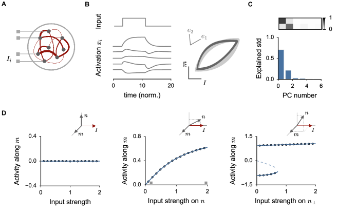
Figure 2: External inputs generate two-dimensional activity in random networks with unit-rank structure. A. The pattern of external inputs can be represented by an $N$-dimensional vector $I=\{I_{i}\}$, where $I_{i}$ is the input to unit $i$. B. Transient dynamics in response to a step input along $I$ in a sample network of $N=3500$ units. Left: activity traces for five units. Right: projections of the population trajectory onto the plane defined by the right-connectivity vector $m$ and the input vector $I$. Light trace: theoretical prediction. Dark traces: simulations. C. Principal components (PC) analysis of the average activity trajectory. Bottom: fraction of standard deviation explained by successive PCs. Top: correlation between PCs and the vectors $m$ and $I$. The direction of the projections onto the $m-I$ plane of the two top PCs $e_{1}$ and $e_{2}$ are represented in B. See also Fig. S3. D. The activity $\kappa$ along $m$ is determined by the geometrical arrangement of the vector $I$ and the connectivity vectors $m$ and $n$. Three different cases are illustrated: (left) $I$, $m$ and $n$ mutually orthogonal; (center) $m$ and $n$ mutually orthogonal, but $I$ has a non-zero overlap with $n$; (right) $m$ and $n$ have non-zero overlap, leading to bistable activity in absence of inputs. Increasing the external input along $n$ suppresses one of the two stable states. Continuous lines: theoretical predictions. Dots: simulations. See Methods for details.

Fig. 2 B illustrates the response of the network to a step input. The response of individual units is highly heterogeneous, different units showing increasing, decreasing or multi-phasic responses. While every unit responds differently, the theory predicts that, at the level of the $N$-dimensional state space representing the activity of the whole population, the trajectory of the activity lies on average on the two-dimensional plane spanned by the right-connectivity vector $m$ and the vector $I=\{I_{i}\}$ that corresponds to the pattern of external inputs (Fig. 2 B). Applying to the simulated activity a dimensionality reduction technique (see Cunningham and Yu (2014) for a recent review) such as Principal Components Analysis confirms that the two dominant dimensions of the activity indeed lie in the $m-I$ plane (Fig. 2 C), while the random part of connectivity leads to additional activity in the remaining $N-2$ directions that grows quickly with the strength of random connectivity $g$ (see Fig. S3). This approach therefore directly links the connectivity in the network to the emerging low-dimensional dynamics, and shows that the dominant dimensions of activity are determined by a combination of feed-forward inputs and connectivity (Wang et al., 2018).

The contribution of the connectivity vector $m$ to the two-dimensional trajectory of activity is quantified by the overlap $\kappa$ between the network activity $[\phi]$ and the left-connectivity vector $n$ (Eq. 4). If $\kappa=0$, the activity trajectory is one-dimensional, and simply propagates the pattern of feed-forward inputs. This is in particular the case for fully random networks. If $\kappa\neq 0$, the network response is instead a non-trivial two-dimensional combination of the input and connectivity structure patterns. In general, the value of $\kappa$, and therefore the organization of network activity, depends on the geometric arrangement of the input vector $I$ with respect to the connectivity vectors $m$ and $n$, as well as on the strength of the random component of the connectivity $g$.

As the neural activity lies predominantly in the $m-I$ plane, a non-vanishing $\kappa$, together with non-trivial two-dimensional activity is obtained when the vector $n$ has a non-zero component in the $m-I$ plane. Two qualitatively different input-output regimes can be distinguished. The first one is obtained when the connectivity vectors $m$ and $n$ are orthogonal to each other (Fig. 2 D left and center). In that case, the overlap between them is zero, and the spontaneous activity in the network bears no sign of the underlying connectivity structure. Adding an external input can, however, reveal this connectivity structure and generate non-trivial two-dimensional activity if the input vector $I$ has a non-zero overlap with the left-connectivity vector $n$. In such a situation, the vector $n$ picks up the component of the activity along the feed-forward input direction $I$. This leads to a non-zero overlap $\kappa$, which in turn implies that the network activity will have a component along the right-connectivity vector $m$. Increasing the external input along the direction of $n$ will therefore progressively increase the response along $m$ (Fig. 2 D center), leading to a two-dimensional output.

A second, qualitatively different input-output regime is obtained when the connectivity vectors $m$ and $n$ have a strong enough overlap along a common direction (Fig. 2 D right). As already shown in Fig. 1, an overlap larger than unity between $m$ and $n$ induces bistable, structured spontaneous activity along the dimension $m$. Adding an external input along the vector $n$ increases the activity along $m$, but also eventually suppresses one of the bistable states. Large external inputs along the $n$ direction therefore reliably set the network into a state in which the activity is a two-dimensional combination of the input direction and the connectivity direction $m$. This can lead to a strongly non-linear input-output transformation if the network was initially set in the state that lies on the opposite branch (Fig. 2 D right).

An additional effect of an external input is that it generally tends to suppress chaotic activity present when the random part of connectivity is strong (Figs. S3 and S4). This suppression occurs irrespectively of the specific geometrical configuration between the input $I$ and connectivity vectors $m$ and $n$, and therefore independently of the two input-output regimes described above. Altogether, external inputs suppress both chaotic and bistable dynamics (Fig. S4), and therefore always decrease the amount of variability in the dynamics (Churchland and al., 2010; Rajan et al., 2010).

In summary, external, feed-forward inputs to a network with unit-rank connectivity structure in general lead to two-dimensional trajectories of activity. The elicited trajectory depends on the geometrical arrangement of the pattern of inputs with respect to the connectivity vectors $m$ and $n$, which play different roles. The right-connectivity vector $m$ determines the output pattern of network activity, while the left-connectivity vector $n$ instead selects the inputs that give rise to outputs along $m$. An output structured along $m$ can be obtained when $n$ selects recurrent inputs (non-zero overlap between $n$ and $m$) or when it selects external inputs (non-zero overlap between $n$ and $I$).

Higher-rank structure leads to a rich dynamical repertoire

This far we focused on unit-rank connectivity structure, but our framework can be directly extended to higher rank structure. A more general structured component of rank $r\ll N$ can be written as a superposition of $r$ independent unit-rank terms

$$P_{ij}=\frac{m_{i}^{(1)}n_{j}^{(1)}}{N}+\ldots+\frac{m_{i}^{(r)}n_{j}^{(r)}}{N},$$ (5)

and is in principle characterized by $2r$ vectors $m^{(k)}$ and $n^{(k)}$. In such a network, the average dynamics lie in the $(r+1)$-dimensional subspace spanned by the $r$ right-connectivity vectors $m^{(k)},k=1,\ldots,r$ and the input vector $I$, while the left connectivity vectors $n^{(k)}$ select the inputs amplified along the corresponding dimension $m^{(k)}$. The details of the dynamics will in general depend on the geometrical arrangement of these $2r$ vectors among themselves and with respect to the input pattern. The number of possible configurations increases quickly with the structure rank, leading to a wide repertoire of dynamical states that includes continuous attractors (Fig. S5) and sustained oscillatory activity (Fig. S8). In the remainder of this manuscript, we will explore only the rank-two case.

Implementing a simple discrimination task

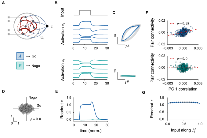
Figure 3: Implementing a simple Go-Nogo discrimination task with a unit-rank connectivity structure. A. A linear readout is added to the network, with randomly chosen weights $w_{i}$. The stimuli are represented by random input patterns $I^{A}$ and $I^{B}$. The task consists in producing an output in response to stimulus $A$, but not $B$. The simplest unit-rank structure that implements the task is given by $m=w$ and $n=I^{A}$. B. Response of a sample network to the Go (blue) and Nogo (green) inputs. Activity traces for five units. C. Projections of the population trajectories onto the planes predicted to contain the dominant part of the dynamics. Gray: predicted trajectory. Colored traces: simulations. D. Linear regression coefficients for the Go and the Nogo stimuli. Every dot corresponds to a network unit. E. Readout dynamics for the Go (blue) and the Nogo (green) stimulus. F. Average connectivity strength as a function of the product between the coefficients of the first PC. Every dot corresponds to a pair of units. G. Generalization properties of the network. We select two Go stimuli $I^{A}_{1}$ and $I^{A}_{2}$, and we set $n=I^{A}_{1}+I^{A}_{2}$. We build the input pattern as a normalized mixture of the two preferred patterns, and we gradually increase the component along $I^{A}_{1}$. Continuous lines: theoretical predictions. Dots: simulations. See Methods for details.

Having developed an intuitive, geometric understanding of how a given unit-rank connectivity structure determines the low-dimensional dynamics in a network, we now reverse our approach to ask how a given computation can be implemented by choosing appropriately the structured part of the connectivity. We start with the computation underlying one of the most basic and most common behavioral tasks, Go-Nogo stimulus discrimination. In this task, an animal has to produce a specific motor output, e.g. press a lever or lick a spout, in response to a stimulus $I^{A}$ (the Go stimulus), and ignore another stimuli $I^{B}$ (Nogo stimuli). This computation can be implemented in a straightforward way in a recurrent network with a unit-rank connectivity structure. While such a simple computation does not in principle require a recurrent network, the implementation we describe here illustrates in a transparent manner the relationship between connectivity, dynamics and computations in low-rank networks, and leads to non-trivial and directly testable experimental predictions. It also provides the basic building block for more complex tasks, which we turn to in the next sections.

We model the sensory stimuli as random patterns of external inputs to the network, so that the two stimuli are represented by two fixed, randomly-chosen $N$-dimensional vectors $I^{A}$ and $I^{B}$. To model the motor response, we supplement the network with an output unit, which produces a linear readout $z(t)=\frac{1}{N}\sum_{i}w_{i}\phi(x_{i}(t))$ of network activity (Fig. 3 A). The readout weights $w_{i}$ are chosen randomly and form also a fixed $N$-dimensional vector $w$. The task of the network is to produce an output that is selective to the Go stimulus: the readout $z$ at the end of stimulus presentation needs to be non-zero for the input pattern $I^{A}$ that corresponds to the Go stimulus, and zero for the other input $I^{B}$.

The two $N$-dimensional vectors $m$ and $n$ that generate the appropriate unit-rank connectivity structure to implement the task can be directly determined from our description of network dynamics. As shown in Eq. 4 and Fig. 2, the response of the network to the input pattern $I$ is in general two-dimensional and lies in the plane spanned by the vectors $m$ and $I$. The output unit will therefore produce a non-zero readout only if the readout vector $w$ has a non-vanishing overlap with either $m$ or $I$. As $w$ is assumed to be uncorrelated, and therefore orthogonal, to all input patterns, this implies that the connectivity vector $m$ needs to have a non-zero overlap with the readout vector $w$ for the network to produce a non-trivial output. This output will depend on the amount of activity along $m$, quantified by the overlap $\kappa$. As shown in Fig. 2, the overlap $\kappa$ will be non-zero only if $n$ has a non-vanishing overlap with the input pattern. Altogether, implementing the Go-Nogo task therefore requires that the right-connectivity vector $m$ is correlated with the readout vector $w$, and that the left-connectivity vector $n$ is correlated with the Go stimulus $I^{A}$.

Choosing $m=w$ and $n=I^{A}$, therefore provides the simplest unit-rank connectivity that implements the desired computation. Fig. 3 illustrates the activity in the corresponding network. At the level of individual units, by construction both stimuli elicit large and heterogeneous responses (Fig. 3 B) that display mixed selectivity (Fig. 3 D). As predicted by the theory, the response to stimulus $B$ is dominantly one-dimensional and organized along the input direction $I^{B}$, while the response to stimulus $A$ is two-dimensional and lies in the plane defined by the right-connectivity vector $m$ and the input direction $I^{A}$ (Fig. 3 C). The readout from the network corresponds to the projection of the activity onto the $m$ direction, and is non-zero only in response to stimulus $A$ (Fig. 3 E), so that the network indeed implements the desired Go-Nogo task. Our framework therefore allows us to directly link the connectivity, the low-dimensional dynamics and the computation performed by the network, and leads to two experimentally testable predictions. The first one is that performing a dimensionality-reduction separately on responses to the two stimuli should lead to larger dimensionality of the trajectories in response to the Go stimulus. The second prediction is that for the Go stimulus, the dominant directions of activity depend on the recurrent connectivity in the network, while for the Nogo stimulus they do not. More specifically, for the activity elicited by the Go stimulus, the dominant principal components are combinations of the input vector $I^{A}$ and right-connectivity vector $m$. Therefore if two neurons have large principal component weights, they are expected to also have large $m$ weights and therefore stronger mutual connections than average (Fig. 3 F top). In contrast, for the activity elicited by the Nogo stimulus, the dominant principal components are determined solely by the feed-forward input, so that no correlation between dominant PC weights and recurrent connectivity is expected (Fig. 3 F bottom). This prediction can in principle be directly tested in experiments analogous to Ko et al. (2011), where calcium imaging in behaving animals is combined with measurements of connectivity in a subset of recorded neurons. Note that in this setup very weak structured connectivity is sufficient to implement computations, so that the expected correlations may be weak if the random part of the connectivity is strong (see Fig. S5).

The unit-rank connectivity structure forms the fundamental scaffold for the desired input-output transform. The random part of the connectivity adds variability around the target output, and can induce additional chaotic fluctuations. Summing the activity of individual units through the readout unit, however, averages out this heterogeneity, so that the readout error decreases with network size as $1/\sqrt{N}$ (Fig. S5). The present implementation is therefore robust to noise, and has desirable computational properties in terms of generalization to novel stimuli. In particular, it can be extended in a straightforward way to the detection of a category of Go stimuli, rather than a single stimulus (Fig. 3 G).

Detection of a noisy stimulus

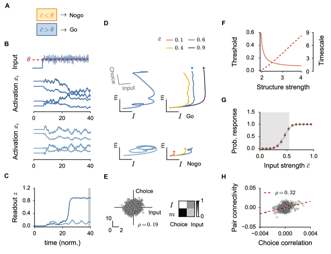
Figure 4: Implementing a noisy detection task with a unit-rank connectivity structure. A. The network is given a noisy input $c(t)$ along a fixed, random pattern of inputs $I$. The task consists in producing an output if the average input $\bar{c}$ is larger than a threshold $\theta$. B. Dynamics in a sample network. Top: noisy input and threshold. Bottom: activity traces for four units and two different noise realizations in the stimulus, leading to a Go (dark blue) and a Nogo (light blue) output. C. Readout dynamics for the two stimuli. D. Projections of the population trajectory onto the plane defined by the right-connectivity vector $m$ and the input vector $I$. Left: single-trial trajectories corresponding to B. Right: trial-averaged trajectories, for Go (top) and Nogo (bottom) outputs, and different values of the mean input $\bar{c}$. Stars indicate correct responses. E. Left: linear regression coefficients for the input amplitude and the decision outcome. Every dot corresponds to a network unit. Right: correlation coefficients between the vectors $m$ and $I$ and the input and choice regression axes (see Methods). Projection directions of the two input and choice regression axes onto the $m-I$ plane are shown in D. F. Detection threshold (dashed), and time scale of the effective exponential filter (full line) for increasing values of the structure strength. G. Psychometric curve. The shaded area indicates the bistable region. H. Average connectivity strength as a function of the product of the linear regression coefficients for the choice variable. Every dot corresponds to a pair of network units. See Methods for details.

We now turn to a slightly more complex task: integration of a continuous, noisy stimulus. In contrast to the previous discrimination task, where the stimuli were completely different (i.e. orthogonal), here we consider a continuum of stimuli that differ only along the intensity of a single feature, such as the coherence of a random-dot kinetogram (Newsome et al., 1989). In a given stimulus presentation, this feature moreover fluctuates in time. We therefore represent each stimulus as $c(t)I$, where $I$ is a fixed, randomly chosen input vector that encodes the relevant stimulus feature, and $c(t)$ is the amplitude of that feature. We consider a Go-Nogo version of this task, in which the network has to produce an output only if the average value of $c$ is larger than a threshold (Fig. 4 A).

As for the basic discrimination task, the central requirements for a unit-rank network to implement this task are that the right-connectivity vector $m$ is correlated with the readout vector $w$, and the left-connectivity vector $n$ is correlated with the input pattern $I$. A key novel requirement in the present task is however that the response needs to be non-linear to produce the Go output when the strength of the input along $I$ is larger than the threshold. As shown in Fig. 2 D, such a non-linearity can be obtained when the left- and right-connectivity vectors $n$ and $m$ have a strong enough overlap. We therefore add a shared component to $m$ and $n$ along a direction orthogonal to both $w$ and $I$. In that setup, if the stimulus intensity $c$ is low, the network will be in a bistable regime, in which the activity along the direction $m$ can take two distinct values for the same input (Fig. 2 D right). Assuming that the lower state represents a Nogo output, and that the network is initialized in this state at the beginning of the trial, increasing the stimulus intensity $c$ above a threshold will lead to a sudden jump, and therefore a non-linear detection of the stimulus. Because the input amplitude fluctuates noisily in time, whether such a jump occurs depends on the integrated estimate of the stimulus intensity. The timescale over which this estimate is integrated is determined by the time-constant of the effective exponential filter describing the network dynamics. In our unit-rank network, this time-constant is set by the connectivity strength, i.e. the overlap between the left- and right-connectivity vectors $m$ and $n$, which also determines the value of the threshold. Arbitrarily large timescales can be obtained by adjusting this overlap close to the bifurcation value, in which case the threshold becomes arbitrarily small (Fig. 4 F). In this section, we fix the structure strength so that the threshold is set to $0.5$, which corresponds to an integration timescale of the order of the time constant of individual units.

Fig. 4 illustrates the activity in an example implementation of this network. In a given trial, as the stimulus is noisy, the activity of the individual units fluctuates strongly (Fig. 4 B). Our theory predicts that the population trajectory on average lies in the plane defined by the connectivity vector $m$ and the input pattern $I$ (Fig. 4 D). Activity along the $m$ direction is picked up by the readout, and its value at the end of stimulus presentation determines the output (Fig. 4 C). Because of the bistable dynamics in the network, whether the $m$ direction is explored, and an output produced, depends on the specific noisy realization of the stimulus. Stimuli with an identical average strength can therefore either lead to two-dimensional trajectories of activity and Go responses, or one-dimensional trajectories of activity corresponding to Nogo responses (Fig. 4 D). The probability of generating an output as function of stimulus strength follows a sigmoidal psychometric curve that reflects the underlying bistability (Fig. 4 G). Note that the bistability is not clearly apparent on the level of individual units. In particular, the activity of individual units is always far from saturation, as their inputs are distributed along a zero-centered Gaussian (Eq. 4).

The responses of individual units are strongly heterogeneous and exhibit mixed selectivity to stimulus strength and output choice (Fig. 4 E). A popular manner to interpret such activity at the population level is a targeted dimensional reduction approach, in which input and choice dimensions are determined through regression analyses (Mante et al., 2013). As expected from our theoretical analysis, the two dimensions obtained through regression are closely related to $m$ and $I$; in particular, the choice dimension is highly correlated with the right-connectivity vector $m$ (Fig. 4 E). As a result, the plane in which network activity dominantly lies corresponds to the plane defined by the choice and the input dimensions (Fig. 4 D). Our framework therefore directly links recurrent connectivity and effective output choice direction through the low-dimensional dynamics. A resulting experimentally testable prediction is that neurons with strong choice regressors have stronger mutual connections (Fig. 4 H).

A context-dependent discrimination task

We next consider a context-dependent discrimination task, in which the relevant response to a stimulus depends on an additional, explicit contextual cue. Specifically, we focus on the task studied in Saez et al. (2015) where in one context (referred to as Context $A$), the stimulus $A$ requires a Go output, and the stimulus $B$ a Nogo, while in the other context (referred to as Context $B$), the associations are reversed (Fig. 5 A). This task is a direct extension of the basic binary discrimination task introduced in Fig. 3, yet it is significantly more complex as it represents a hallmark of cognitive flexibility: a non-linearly separable, $XOR$-like computation that a single-layer feed-forward network cannot solve (Rigotti et al., 2010; Fusi et al., 2016). We will show that this task can be implemented in a rank-two recurrent network that is a direct extension of the unit-rank network used for the discrimination task in Fig. 4.

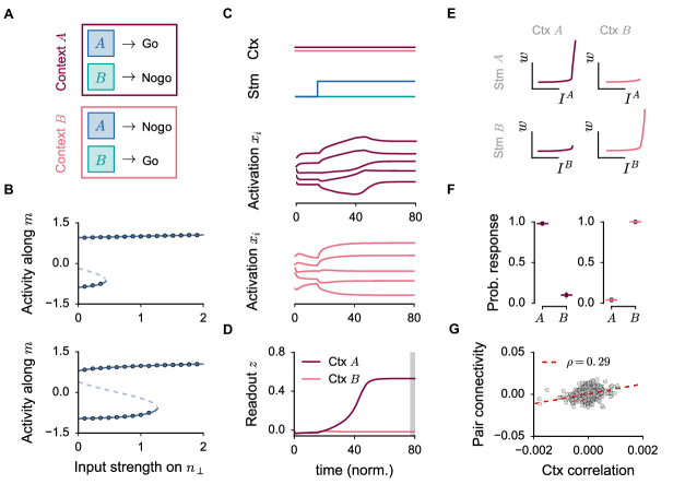
Figure 5: Implementing a context-dependent Go-Nogo discrimination task with a rank-two connectivity structure. A. As in Fig. 3, two stimuli $A$ and $B$ are presented to the network. The task consists in producing an output in response to the Go stimulus, which is determined by the contextual cue ($A$ in Context $A$, $B$ in Context $B$), modeled as inputs along random directions $I_{ctxA}$ and $I_{ctxB}$. B. Inputs along the overlap direction between the left- and the right-connectivity vectors modulate the response threshold of the network (see also Fig. S5). C. Dynamics in a sample network in response to the stimulus $A$. Top: stimulus and contextual input. Bottom: activity for five units in contexts $A$ (crimson) and $B$ (pink). D. Readout dynamics in the two contexts. E. Projections of the average population trajectories onto the planes spanned by vectors $w$, $I^{A}$ and $I^{B}$. F. Network performance in the two contexts. G. Average connectivity strength between pairs of units as a function of the product between the regression coefficients for context. Every dot corresponds to a pair of network units. See Methods for details.

This context-dependent task can be seen as a combination of two basic, opposite Go-Nogo discriminations, each of which can be independently implemented by a unit-rank structure with the right-connectivity vector $m$ correlated to the readout, and the left-connectivity vector correlated to the Go input ($I^{A}$ for Context $A$, $I^{B}$ for Context $B$). Combining two such unit-rank structures, with left-connectivity vectors $n^{(1)}$ and $n^{(2)}$ correlated respectively with $I^{A}$ and $I^{B}$, leads to a rank-two connectivity structure that serves as a scaffold for the present task. The cues for context $A$ and $B$ are represented by additional inputs along random vectors $I_{ctxA}$ and $I_{ctxB}$, presented for the full length of the trial (Remington et al., 2018) (Fig. 5 C). These inputs are the only contextual information incorporated in the network. In particular, the readout vector $w$ is fixed and independent of the context (Mante et al., 2013). Crucially, since the readout $w$ needs to produce an output for both input stimuli, both right-connectivity vectors $m^{(1)}$ and $m^{(2)}$ need to be correlated with it.

The key requirement for implementing context-dependent discrimination is that each contextual input effectively switches off the irrelevant association. To implement this requirement, we rely on the same non-linearity as for the noisy discrimination task, based on the overlap between the left- and right-connectivity vectors (Fig. 2 D). We however exploit an additional property, which is that the threshold of the non-linearity (i.e. the position of the transition from a bistable to a mono-stable region in Fig. 2 D) can be controlled by an additional modulatory input along the overlap direction between $m$ and $n$ (Figs. 5 B and S4). Such a modulatory input acts as an effective offset for the bistability at the macroscopic, population level (see Eq. 153 in Methods). A stimulus of a given strength (e.g. unit strength in Fig. 5 B) may therefore induce a transition from the lower to the upper state (Fig. 5 B top), or no transition (Fig. 5 B bottom) depending on the strength of the modulatory input that sets the threshold value. While in the noisy discrimination task, the overlap between $m$ and $n$ was chosen in an arbitrary direction, in the present setting we take the overlaps between each pair of left- and right-connectivity vectors to lie along the direction of the corresponding contextual input (i.e. $m^{(1)}$ and $n^{(1)}$ overlap along $I_{ctxA}$, $m^{(2)}$ and $n^{(2)}$ along $I_{ctxB}$), so that contextual inputs directly modulate the threshold of the non-linearity. The final rank-two setup is described in detail in the Methods.

Fig. 5 illustrates the activity in an example of the resulting network implementation. The contextual cue is present from the very beginning of the trial, and effectively sets the network in a context-dependent initial state (Fig. 5 C) that corresponds to the lower of the two bistable states. The low-dimensional response of the network to the following stimulus is determined by this initial state and the sustained contextual input. If the cue for context $A$ is present, stimulus $A$ leads to the crossing of the non-linearity, a transition from the lower to the upper state, and therefore a two-dimensional response in the plane determined by $I^{A}$ and $w$ (Figs. 5 E top left), generating a Go output (Fig. 5 D). In contrast, if the cue for context $B$ is present, the threshold of the underlying non-linearity is increased in the direction of input $I^{A}$ (Fig. 5 B bottom), so that the presentation of stimulus $A$ does not induce a transition between the lower and upper states, but leads only to a one-dimensional trajectory orthogonal to the readout, and therefore a Nogo response (Fig. 5 E top right). The situation is totally symmetric in response to stimulus $B$ (Fig. 5 E bottom), so that contextual cues fully reverse the stimulus-response associations (Fig. 5 F). Overall, this context-dependent discrimination relies on strongly non-linear interactions between the stimulus and contextual inputs, that on the connectivity level are implemented by overlaps between the connectivity vectors along the contextual inputs. A central, experimentally testable prediction of our framework is therefore that, if a network is implementing this computation, units with strong contextual selectivity have on average stronger mutual connections (Fig. 5 G).

A context-dependent evidence integration task

We finally examine a task inspired by Mante et al. (2013) that combines context-dependent output and fluctuating, noisy inputs. The stimuli now consist of superpositions of two different features $A$ and $B$, and the strengths of both features fluctuate in time during a given trial. In Mante et al. (2013), the stimuli were random dot kinetograms, and the features $A$ and $B$ corresponded to the direction of motion and color of these stimuli. The task consists in classifying the stimuli according to one of those features, the relevant one being indicated by an explicit contextual cue (Fig. 6 A).

We implemented a Go-Nogo version of the task, in which the output is required to be non-zero when the relevant feature is stronger than a prescribed threshold (arbitrarily set to $0.5$). The present task is therefore a direct combination of the detection task introduced in Fig. 4 and the context-dependent discrimination task of Fig. 5, but the individual stimuli are now two-dimensional, as they consist of two independently varied features $A$ and $B$. In this task, a significant additional difficulty is that on every trial the irrelevant feature needs to be ignored, even if it is stronger than the relevant feature (e.g. color coherence stronger than motion coherence on a motion-context trial).

This context-dependent evidence integration task can be implemented with exactly the same rank-two configuration as the basic context-dependent discrimination in Fig. 5, with contextual gating relying on the same non-linear mechanism as in Fig. 5 B. The contextual cue is presented throughout the trial (Fig. 6 B), and determines which of the features of the two-dimensional stimulus leads to non-linear dynamics along the direction of connectivity vectors $m^{(1)}$ and $m^{(2)}$ (Fig. 6 D). These directions share a common component along the readout vector $w$, and the readout unit picks up the activity along that dimension. As a consequence, depending on the contextual cue, the same stimulus can lead to opposite outputs (Fig. 6 C). Altogether, in Context $A$, the output is independent of the values of feature $B$, and conversely in Context $B$ (Fig. 6 E). The output therefore behaves as if it were based on two orthogonal readout directions, yet the readout direction is unique and fixed, and the output relies instead on a context-dependent selection of the relevant input feature (Mante et al., 2013).

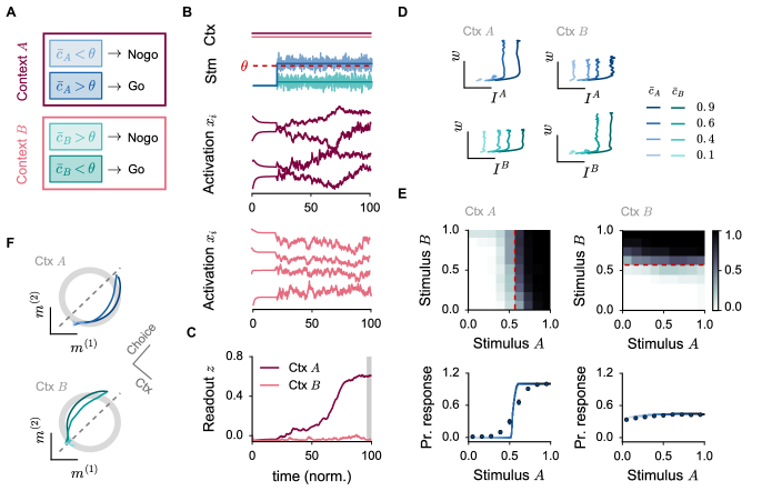
Figure 6: Implementing a context-dependent evidence accumulation task using rank-two connectivity structure. A. The stimuli consist of a superposition of two features $c_{A}$ and $c_{B}$ which fluctuate in time around mean values $\bar{c}_{A}$ and $\bar{c}_{B}$. In every trial, a pair of contextual inputs determines the relevant input feature. The task consists in producing an output if the average strength of the relevant feature is larger than a threshold. B. Dynamics in a sample network. Top: stimulus and contextual inputs. Bottom: activity of four units in contexts A (crimson) and B (pink). C. Readout dynamics in the two contexts. D. Average population trajectories projected onto the planes spanned by vectors $w$, $I^{A}$ and $I^{B}$. Blue (resp. green) trajectories have been sorted according to the value of the strength of stimulus $A$ (resp. $B$), and averaged across stimulus $B$ (resp. $A$). E. Network performance. Top row: probability of response as function of input strengths $\bar{c}_{A}$ and $\bar{c}_{B}$ (simulated data). Bottom: probability of response averaged over $\bar{c}_{B}$. Continuous line: theoretical prediction; dots: simulations. F. Projection of the population activity onto the plane defined by the orthogonal components of the vectors $m^{(1)}$ and $m^{(2)}$ , and comparison with the underlying circular attractor (see Methods). Trajectories are sorted by the strength of the relevant stimulus, and averaged across the non-relevant one. The direction of the projections of the regression axes for choice and context are indicated in gray. See Methods for details.

An important additional requirement in the present task with respect to the basic context-dependent integration is that the network needs to perform temporal integration to average out temporal fluctuations in the stimulus. As illustrated in Fig. 6 B-C, the network dynamics in response to stimuli indeed exhibit a slow timescale, and progressively integrate the input. Strikingly, such slow dynamics do not require additional constraints on network connectivity; they are a direct consequence of the rank-two connectivity structure used for contextual gating (in fact the dynamics are already slow in the basic contextual discrimination task, see Fig. 5 C-D). More specifically, the symmetry between the two contexts implies that two sets of left- and right- connectivity vectors have identical overlaps (i.e. $m^{(1)T}n^{(1)}=m^{(2)T}n^{(2)}$). Without further constraints on the connectivity, such a symmetric configuration leads to an emergence of a continuous line attractor, with the shape of a two-dimensional ring in the plane defined by $m^{(1)}$ and $m^{(2)}$ (see Methods and Fig. S5). In the implementation of the present task, on top of symmetric overlaps, the four connectivity vectors include a common direction along the readout vector. This additional constraint eliminates the ring attractor, and stabilizes only two equilibrium states that correspond to Go and Nogo outputs. Yet, the ring attractor is close in parameter space, and this proximity induces a slow manifold in the dynamics, so that the trajectories leading to a Go output slowly evolve along two different sides of the underlying ring depending on the context (Fig. 6 F). As a result, the two directions in the plane $m^{(1)}-m^{(2)}$ correspond to choice and context axis as found by regression analysis (Fig. 6 F). A similiar mechanism for context-dependent evidence integration based on a line attractor was previously identified by reverse-engineering a trained recurrent network (Mante et al., 2013). Whether the underlying dynamical structure was a ring as in our case, or two line attractors for the two contexts depended on the details of the network training protocol (V. Mante, Cosyne 2018). Here we show that such a mechanism based on a ring attractor can be implemented in a minimal network with rank-two connectivity structure, but other solutions can certainly be found. Note that this rank-two network can also serve as an alternative implementation for context-independent evidence integration in which the integration timescale and the threshold value are fully independent in contrast to the unit-rank implementation (Fig. 4).

Discussion

Motivated by the observation that a variety of approaches for implementing computations in recurrent networks rely on a common type of connectivity structure, we studied a class of models in which the connectivity matrix consists of a sum of a fixed, low-rank term and a random part. Our central result is that the low-rank connectivity structure induces low-dimensional dynamics in the network, a hallmark of population activity recorded in behaving animals (Gao and Ganguli, 2015). While low-dimensional activity is usually detected numerically using dimensional-reduction techniques (Cunningham and Yu, 2014), we showed that a mean-field theory allows us to directly predict the low-dimensional dynamics based on the connectivity and input structure. This approach led us to a simple, geometrical understanding of the relationship between connectivity and dynamics, and enabled us to design minimal-connectivity implementations of specific computations. In particular, we found that the dynamical repertoire of the network increases quickly with the rank of the connectivity structure, so that rank-two networks can already implement a variety of computations. In this study, we have not explicitly considered structures with rank higher than two, but our theoretical framework is in principle valid for arbitrary rank $r\ll N$, where $N$ is the size of the network.

While other works have examined dynamics in networks with a mixture of structured and random connectivity (e.g. Roudi and Latham (2007); Ahmadian et al. (2015)), the most classical approach for implementing computations in recurrent networks has been to endow them with a clustered (Wang, 2002; Amit and Brunel, 1997; Litwin-Kumar and Doiron, 2012) or distance-dependent connectivity (Ben-Yishai et al., 1995). Such networks inherently display low-dimensional dynamics similar to our framework (Doiron and Litwin-Kumar, 2014; Williamson et al., 2016), as clustered connectivity is in fact a special case of low-rank connectivity. Clustered connectivity, however, is highly ordered: each neuron belongs to a single cluster and therefore is selective to a single task feature (e.g. a given stimulus, or a given output). Neurons in clustered networks are therefore highly specialized and display pure selectivity (Rigotti et al., 2013). Here, instead, we have considered random low-rank structures, which generate activity organized along heterogeneous directions in state space. As a consequence, stimuli and outputs are represented in a random, highly distributed manner and individual neurons are typically responsive to several stimuli, outputs, or combinations of the two. Such mixed selectivity is a ubiquitous property of cortical neurons (Rigotti et al., 2013; Mante et al., 2013; Churchland and Shenoy, 2007), and confers additional computational properties to our networks (Kanerva, 2009). In particular, it allowed us to easily extend to a context-dependent situation (Mante et al., 2013; Saez et al., 2015) a network implementation of a basic discrimination task. This is typically difficult to do in clustered, purely selective networks (Rigotti et al., 2010).

The type of connectivity used in our study is closely related to the classical framework of Hopfield networks (Hopfield, 1982; Amit et al., 1985). The aim of Hopfield networks is to store in memory specific patterns of activity by creating for each pattern a corresponding fixed-point in the network dynamics. This is achieved by adding a unit-rank term for each item, and one approach for investigating the capacity of such a setup has relied on the mean-field theory of a network with a connectivity that consists of a sum of a rank-one term and a random matrix (Tirozzi and Tsodyks, 1991; Shiino and Fukai, 1993; Roudi and Latham, 2007). While this approach is clearly close to the one adopted in the present study, there are important differences. Within Hopfield networks, the unit-rank terms are symmetric, so that the corresponding left- and right-connectivity vectors are identical for each pattern. Moreover, the unit-rank terms that correspond to different patterns are generally uncorrelated. In contrast, here we have considered the more general case where the left- and right-eigenvectors are different, and potentially correlated between different rank-one terms. Most importantly, our main focus was on responses to external inputs and input-output computations, rather than memorizing items. In particular we showed that left- and right-connectivity vectors play different roles with respect to processing inputs, with the left-connectivity vector implementing input- selection, and the right-connectivity vector determining the output of the network.

Our study is also directly related to echo-state networks (ESN) (Jaeger and Haas, 2004) and FORCE learning (Sussillo and Abbott, 2009). In those frameworks, randomly connected recurrent networks are trained to produce specified outputs using a feedback loop from a readout unit to the network, which is mathematically equivalent to adding a rank-one term to the random connectivity matrix (Maass et al., 2007). In their most basic implementation, both ESN and FORCE learning train only the readout weights. The training is performed for a fixed, specified realization of the random connectivity, so that the final rank-one structure is correlated with the random part of the connectivity and may be strong with respect to it. In contrast, the results presented here rely on the assumption that the low-rank structure is weak and independent from the random part. Although ESN and FORCE networks do not necessarily fulfill this assumption, in ongoing work we found that our approach describes well networks trained using ESN or FORCE to produce a constant output (Rivkind and Barak, 2017). Note that in our framework, the computations rely solely on the structured part of the connectivity, but ongoing work suggests that the random part of the connectivity may play an important role during training.

The specific network model used here is identical to most studies based on trained recurrent networks (Sussillo and Abbott, 2009; Mante et al., 2013; Sussillo, 2014). It is highly simplified and lacks many biophysical constraints, the most basic ones being positive firing rates, the segregation between excitation and inhibition and interactions through spikes. Recent works have investigated extensions of the abstract model used here to networks with biophysical constraints (Ostojic, 2014; Kadmon and Sompolinsky, 2015; Harish and Hansel, 2015; Mastrogiuseppe and Ostojic, 2017; Thalmeier et al., 2016). Additional work will be needed to implement the present framework in networks of spiking neurons.

Our results imply novel, directly testable experimental predictions relating connectivity, low-dimensional dynamics and computational properties of individual neurons. Our main result is that the dominant components of low-dimensional dynamics are a combination of feed-forward input patterns, and vectors specifying the low-rank recurrent connectivity (Fig. 2 C). A direct implication is that, if the low-dimensional dynamics in the network are generated by low-rank recurrent connectivity, two neurons that have large loadings in the dominant principal components will tend to have mutual connections stronger than average (Fig. 3 F top). In contrast, if the low-dimensional dynamics are not generated by recurrent interactions, but instead driven by feed-forward inputs alone, no correlation between principal components and connectivity is expected (Fig. 3 F bottom). Since the low-dimensional dynamics based on recurrent connectivity form the scaffold for computations in our model, this basic prediction can be extended to various task-dependent properties of individual neurons. For instance, if the recurrent connectivity implements evidence integration, two units with strong choice regressors are predicted to have mutual connections stronger than average (Fig. 4 H). Analogously, if recurrent connections implement context-dependent associations, two units with strong context regressors are expected to share connections stronger than average (Fig. 5 G). Such predictions can in principle be directly tested in experiments that combine calcium imaging of neural activity in behaving animals with measurements of connectivity between a subset of recorded neurons (Ko et al., 2011). It should be noted however that very weak structured connectivity is sufficient to implement computations, so that the expected correlations between connectivity and various selectivity indices may be weak.

The class of recurrent networks we considered here is based on connectivity matrices that consist of an explicit sum of a low-rank and a random part. While this may seem as a limited class of models, in fact any arbitrary matrix can be approximated with a low-rank one, e.g. by keeping a small number of dominant singular values and singular vectors (Markovsky, 2012) – this is the basic principle underlying dimensionality reduction. A recurrent network with any arbitrary connectivity matrix can therefore in principle be approximated by a low-rank recurrent network. From this point of view, our theory suggests a simple conjecture: the low-dimensional structure in connectivity determines low-dimensional dynamics and computational properties of recurrent networks. While more work is needed to establish under which precise conditions a low-rank network provides a good computational approximation of a full recurrent network, this conjecture provides a simple and practically useful working hypothesis for reverse-engineering trained neural networks (Sussillo and Barak, 2012), and relating connectivity, dynamics and computations in neural recordings.

Author contributions

F.M. and S.O. designed the study and wrote the manuscript. F.M. performed model analyses and simulations.

Declaration of Interests

The authors declare no competing interests.

STAR Methods

Contact for Reagent and Resource Sharing

Further requests for resources should be directed to and will be fulfilled by the Lead Contact, Srdjan Ostojic (srdjan.ostojic@ens.fr).

Method Details

The network model

We study large recurrent networks of rate units. Every unit in the network is characterized by a continuous variable $x_{i}(t)$, commonly interpreted as the total input current. More generically, we also refer to $x_{i}(t)$ as the activation variable. The output of each unit is a non-linear function of its inputs modeled as a sigmoidal function $\phi(x)$. In line with previous works (Sompolinsky et al., 1988; Sussillo and Abbott, 2009; Rivkind and Barak, 2017), we focus on $\phi(x)=\tanh(x)$, but we show that qualitatively similar dynamical regimes appear in network models with more realistic, positively defined activation functions (Fig. S7). The transformed variable $\phi(x_{i}(t))$ is interpreted as the firing rate of unit $i$, and is also referred to as the activity variable.

The time evolution is specified by the following dynamics:

$$\dot{x}_{i}(t)=-x_{i}(t)+\sum_{j=1}^{N}J_{ij}\phi(x_{j}(t))+I_{i}.$$ (6)

We considered a particular class of connectivity matrices, which can be written as a sum of two terms:

$$J_{ij}=g\chi_{ij}+P_{ij}.$$ (7)

Similarly to (Sompolinsky et al., 1988), $\chi_{ij}$ is a Gaussian all-to-all random matrix, where every element is drawn from a centered normal distribution with variance $1/N$. The parameter $g$ scales the strength of random connections in the network, and we refer to it also as the random strength. The second term $P_{ij}$ is a low-rank matrix. In this study, we consider the low-rank part of the connectivity fixed, while the random part varies between different realizations of the connectivity. Our results rely on two simplifying assumptions. The first one is that the low-rank term and the random term are statistically uncorrelated. The second one is that, as stated in Eq. 8, the structured connectivity is weak in the large $N$ limit, i.e. it scales as $1/N$, while the random connectivity components $\chi_{ij}$ scale as $1/\sqrt{N}$.

We first consider the simplest case where $P_{ij}$ is a rank-one matrix, which can generally be written as the external product between two one-dimensional vectors $m$ and $n$:

$$P_{ij}=\frac{m_{i}n_{j}}{N}.$$ (8)

According to our first assumption, the entries of vectors $m$ and $n$ are independent of the random bulk of the connectivity $\chi_{ij}$. Note that the only non-zero eigenvalue of $P$ is given by the scalar product $m^{T}n/N$, and the corresponding right and left eigenvectors are, respectively, vectors $m$ and $n$. In the following, we will refer to the eigenvalue $m^{T}n/N$ as the strength of the connectivity structure, and to $m$ and $n$ as the right- and left-connectivity vectors. Here we focus on vectors obtained by generating the components from a joint Gaussian distribution.

More general connectivity structures of rank $r\ll N$ can be written as a sum of unit-rank terms

$$P_{ij}=\frac{m_{i}^{(1)}n_{j}^{(1)}}{N}+\ldots+\frac{m_{i}^{(r)}n_{j}^{(r)}}{N},$$ (9)

and are therefore specified by $r$ pairs of vectors $m^{(k)}$ and $n^{(k)}$, where different $m$ vectors are linearly independent, and similarly for $n$ vectors.

Overview of Dynamical Mean-Field theory

Our results rely on a mathematical analysis of network dynamics based on Dynamical Mean-Field (DMF) theory (Sompolinsky et al., 1988; Rajan et al., 2010; Kadmon and Sompolinsky, 2015). To help navigate the analysis, here we provide first a succint overview of the approach. Full details are given further down in the section Details of Dynamical Mean-Field theory.

DMF theory allows one to derive an effective description of the dynamics by averaging over the disorder originating from the random part of the connectivity. Across different realizations of the random connectivity matrix $\chi_{ij}$, the sum of inputs to unit $i$ is approximated by a Gaussian stochastic process $\eta_{i}(t)$

$$\sum_{j=1}^{N}J_{ij}\phi(x_{j}(t))+I_{i}\approx\eta_{i}(t),$$ (10)

so that each unit obeys a Langevin-like equation:

$$\dot{x}_{i}(t)=-x_{i}(t)+\eta_{i}(t).$$ (11)

The Gaussian processes $\eta_{i}$ can in principle have different first and second-order statistics for each unit, but are otherwise statistically independent across different units. As a consequence, the activations $x_{i}$ of different units are also independent Gaussian stochastic processes, coupled only through their first and second-order statistics. The core of DMF theory consists of self-consistent equations for the mean $\mu_{i}$ and auto-correlation function $\Delta^{I}_{i}(t)$.

At equilibrium (i.e. in absence of transient dynamics) the equation for the mean $\mu_{i}$ of $x_{i}$ is obtained by directly averaging Eq. 6 over the random part of the connectivity. For a unit-rank connectivity, it reads

$$\mu_{i}=\kappa m_{i}+I_{i},$$ (12)

where

$$\kappa=\frac{1}{N}\sum_{j=1}^{N}n_{j}\big{[}\phi_{j}\big{]}.$$ (13)

In the last equation, we adopted the short-hand notation $\phi_{i}(t)\coloneqq\phi(x_{i}(t))$. Here $\big{[}\phi_{j}\big{]}$ is the average firing rate of unit $j$, i.e. $\phi(x_{j})$ averaged over the Gaussian variable $x_{j}$. In a geometrical interpretation, the quantity $\kappa$ represents the overlap between the left-connectivity vector $n$ and the vector of average firing rates. Equivalently, it is given by a population average of $n_{j}\big{[}\phi_{j}\big{]}$, which can also be expressed as

$$\kappa=\int\mathop{}\!\mathrm{d}m\mathop{}\!\mathrm{d}n\mathop{}\!\mathrm{d}I\>p(m,n,I)\>n\int\mathcal{D}z\phi(m\kappa+I+\sqrt{\Delta_{0}^{I}}z)$$ (14)

where $p(m,n,I)$ is the joint distribution of components of vectors $m$, $n$ and $I$. $\Delta_{0}^{I}$ is the variance of $x_{i}$ (see below), and $\int\mathcal{D}z=\int_{-\infty}^{+\infty}\frac{e^{-\frac{z^{2}}{2}}}{\sqrt{2\pi}}\mathop{}\!\mathrm{d}z$.

The auto-correlation function $\Delta^{I}_{i}(t)$ quantifies the fluctuations of the activation $x_{i}$ around the expected mean. Computing this auto-correlation function shows that it is identical for all units in the network, i.e. independent of $i$ (see Eq. 27). It can be decomposed into a static variance, which quantifies the fluctuations of the equilibrium values of $x_{i}$ across different realizations of the random component of the connectivity, and an additional temporal variance which is present when the network is in a temporally fluctuating, chaotic state. In a stationary state, the variance $\Delta^{I}_{0}\equiv\Delta^{I}(t=0)$ can be expressed as

$$\Delta_{0}^{I}=g^{2}\frac{1}{N}\sum_{j=1}^{N}[\phi_{i}^{2}].$$ (15)

where $[\phi_{i}^{2}]$ is the average of $\phi_{i}^{2}(x)$ over the Gaussian variable $x_{i}$.

The right-hand-sides of Eqs. 13 and 15 show that both the mean $\mu_{i}$ and variance $\Delta_{0}^{I}$ depend on population-averaged, macroscopic quantities. To fully close the DMF description, the equations for single-unit statistics need to be averaged over the population. For static equilibrium dynamics, this leads to two coupled equations for two macroscopic quantities, the overlap $\kappa$ and the static, population-averaged variance $\Delta_{0}$:

$$\begin{split}&\kappa=F(\kappa,\Delta_{0})\\ &\Delta_{0}=G(\kappa,\Delta_{0}).\end{split}$$ (16)

Here $F$ and $G$ are two non-linear functions, the specific form of which depends on the geometrical arrangement of the connectivity vectors $m$ and $n$ and the input vector $I$. For temporally fluctuating, chaotic dynamics an additional macroscopic quantity (corresponding to the temporal variance) needs to be taken into account. In that case, the full DMF description is given by a system of three non-linear equations for three unknowns. The equilibrium states of the network dynamics are therefore obtained by solving these systems of equations using standard non-linear methods.

To describe the transient dynamics and assess the stability of the obtained equilibrium states, we determined the spectrum of eigenvalues at the obtained equilibrium fixed points. This spectrum consists of two components: a continuous, random component distributed within a circle in the complex plane, and a single outlier induced by the structured part of the connectivity (Fig. S1 A, D). The radius of the continuous component and the value of the outlier depend on the connectivity parameters. Although the two quantities in general are non-trivially coupled, the value of the radius is mostly controlled by the strength of the disorder, while the value of the outlier increases with the strength $m^{T}n/N$ of the rank-one structure (Fig. S1 F). The equilibrium is stable as long as the real part of all eigenvalues is less than unity. For large connectivity structure strengths, the outlier crosses unity, generating an instability that leads to the appearance of one-dimensional structured activity. Increasing the disorder strength on the other hand leads to another instability, corresponding to the radius of the continuous component crossing unity. This instability gives rise to chaotic, fluctuating activity.

When a linear readout with weights $w_{i}$ is added to the network, its average output is given by

$$z(t)=\frac{1}{N}\sum_{i=1}^{N}w_{i}\big{[}\phi_{i}(t)\big{]},$$ (17)

i.e. by the projection of the average network firing rate on the readout vector $w$. This quantity is analogous to $\kappa$, except that the vector $n$ is replaced by the vector $w$, so that similarly to Eq. 14, the average readout can also be expressed as

$$z=\int\mathop{}\!\mathrm{d}m\mathop{}\!\mathrm{d}w\mathop{}\!\mathrm{d}I\>p(m,w,I)\>w\int\mathcal{D}y\phi(m\kappa+I+\sqrt{\Delta_{0}^{I}}y)$$ (18)

and therefore directly depends on the joint distribution $p(m,w,I)$ which characterizes the geometric arrangement of vectors $m$, $w$ and $I$.

The DMF theory can be directly extended to connectivity structures of rank $r$ greater than one. The equilibrium mean input to unit $i$ is then given by

$$\mu_{i}=\sum_{k=1}^{r}\kappa^{(k)}m_{i}^{(k)}+I_{i}.$$ (19)

The activity therefore lives in an $(r+1)$-dimensional space determined by the $r$ right-connectivity vectors $m^{(k)}$ and the input vector $I$. It is characterized by $r$ overlaps $\kappa^{(k)}$, each of which quantifies the amount of activity along the corresponding direction $m^{(k)}$. Averaging over the population, the DMF theory then leads to a system of $r+1$ nonlinear coupled equations for describing stationary dynamics.

Details of Dynamical Mean-Field theory

Here we provide the full details of the mathematical analysis. We start by examining the activity of a network with a rank-one structure in absence of external inputs ($I_{i}=0$ $\forall i$ in Eq. 6).

Single-unit equations for spontaneous dynamics

We start by determining the statistics of the effective noise $\eta_{i}$ to unit $i$, defined by

$$\eta_{i}(t)=g\sum_{j=1}^{N}\chi_{ij}\phi(x_{j}(t))+\frac{m_{i}}{N}\sum_{j=1}^{N}n_{j}\phi(x_{j}(t)).$$ (20)

The DMF theory relies on the hypothesis that a disordered component in the coupling structure, here represented by $\chi_{ij}$, efficiently decorrelates single neuron activity when the network is sufficiently large. We will show that this hypothesis of decorrelated activity is self-consistent for the specific network architecture we study.

As in standard DMF derivations, we characterize self-consistently the distribution of $\eta_{i}$ by averaging over different realizations of the random matrix $\chi_{ij}$ (Sompolinsky et al., 1988; Rajan et al., 2010). In the following, $[.]$ indicates an average over the realizations of the random matrix $\chi_{ij}$, while $\langle.\rangle$ stands for an average over different units of the network. Note that the network activity can be equivalently characterized in terms of input current variables $x_{i}(t)$ or their non-linear transforms $\phi(x_{i}(t))$. As these two quantities are not independent, the statistics of the distribution of the latter can be written in terms of the statistics of the former.

The mean of the effective noise received by unit $i$ is given by:

$$[\eta_{i}(t)]=g\sum_{j=1}^{N}[\chi_{ij}\phi(x_{j}(t))]+\frac{m_{i}}{N}\sum_{j=1}^{N}n_{j}[\phi(x_{j}(t))].$$ (21)

Under the hypothesis that in large networks, neural activity decorrelates (more specifically, that activity $\phi(x_{j}(t))$ is independent of its outgoing weights), we have:

$$[\eta_{i}(t)]=g\sum_{j=1}^{N}[\chi_{ij}][\phi(x_{j}(t))]+\frac{m_{i}}{N}\sum_{j=1}^{N}n_{j}[\phi(x_{j}(t))]=m_{i}\kappa$$ (22)

as $[\chi_{ij}]=0$. Here we introduced

$$\kappa\coloneqq\frac{1}{N}\sum_{j=1}^{N}n_{j}[\phi(x_{j}(t))]=\langle n_{j}[\phi_{j}(t)]\rangle,$$ (23)

which quantifies the overlap between the mean population activity vector and the left-connectivity vector $n$.

Similarly, the noise correlation function is given by

$$\begin{split}[\eta_{i}(t)\eta_{j}(t+\tau)]=&g^{2}\sum_{k=1}^{N}\sum_{l=1}^{N}[\chi_{ik}\chi_{jl}][\phi(x_{k}(t))\phi(x_{l}(t+\tau))]\\ &+\frac{m_{i}m_{j}}{N^{2}}\sum_{k=1}^{N}\sum_{l=1}^{N}n_{k}n_{l}[\phi(x_{k}(t))\phi(x_{l}(t+\tau))].\end{split}$$ (24)

Note that every cross-term in the product vanishes since $[\chi_{ij}]=0$. Similarly to standard DMF derivations (Sompolinsky et al., 1988), the first term on the r.h.s. vanishes for cross-correlations ($i\neq j$) while it survives in the auto-correlation function ($i=j$), as $[\chi_{ik}\chi_{jl}]={\delta_{ij}\delta_{kl}}/{N}$. We get:

$$[\eta_{i}(t)\eta_{j}(t+\tau)]=\delta_{ij}g^{2}\langle[\phi_{i}(t)\phi_{i}(t+\tau)]\rangle+\frac{m_{i}m_{j}}{N^{2}}\sum_{k=1}^{N}\sum_{l=1}^{N}n_{k}n_{l}[\phi(x_{k}(t))\phi(x_{l}(t+\tau))].$$ (25)

We focus now on the second term in the right-hand side. The corresponding sum contains $N$ terms where $k=l$. This contribution vanishes in the large $N$ limit because of the $1/N^{2}$ scaling. According to our starting hypothesis, when $k\neq l$, activity decorrelates: $[\phi_{k}(t)\phi_{l}(t+\tau)]=[\phi_{k}(t)][\phi_{l}(t+\tau)]$. To the leading order in $N$, we get:

$$\begin{split}[\eta_{i}(t)\eta_{j}(t+\tau)]&=\delta_{ij}g^{2}\langle[\phi_{i}(t)\phi_{i}(t+\tau)]\rangle+\frac{m_{i}m_{j}}{N^{2}}\sum_{k}n_{k}[\phi(x_{k}(t))]\sum_{l\neq k}n_{l}[\phi(x_{l}(t+\tau))]\\ &=\delta_{ij}g^{2}\langle[\phi_{i}(t)\phi_{i}(t+\tau)]\rangle+m_{i}m_{j}\kappa^{2}\end{split}$$ (26)

so that:

$$[\eta_{i}(t)\eta_{j}(t+\tau)]-[\eta_{i}(t)][\eta_{j}(t)]=\delta_{ij}g^{2}\langle[\phi_{i}(t)\phi_{i}(t+\tau)]\rangle.$$ (27)

We therefore find that the statistics of the effective input are uncorrelated across different units, so that our initial hypothesis is self-consistent.

To conclude, for every unit $i$, we computed the first- and the second-order statistics of the effective input $\eta_{i}(t)$. The expressions we obtained show that the individual noise statistics depend on the statistics of the full network activity. In particular, the mean of the effective input depends on the average overlap $\kappa$, but varies from unit to unit through the components of the right-connectivity vector $m$. On the other hand, the auto-correlation of the effective input is identical for all units, and determined by the population-averaged firing rate auto-correlation $\langle[\phi_{i}(t)\phi_{i}(t+\tau)]\rangle$.

Once the statistics of $\eta_{i}(t)$ have been determined, a self-consistent solution for the activation variable $x_{i}(t)$ can be derived by solving the Langevin-like stochastic process from Eq. 11. As a first step, we look at its stationary solutions, which correspond to the fixed points of the original network dynamics.

Population-averaged equations for stationary solutions

For any solution that does not depend on time, the mean $\mu_{i}$ and the variance $\Delta_{0}^{I}$ of the variable $x_{i}$ with respect to different realizations of the random connectivity coincide with the statistics of the effective noise $\eta_{i}$. From Eqs. 22 and 27, the mean $\mu_{i}$ and variance $\Delta_{0}^{I}$ of the input to unit $i$ therefore read

$$\begin{split}&\mu_{i}\coloneqq[x_{i}]=m_{i}\kappa\\ &\Delta_{0}^{I}\coloneqq[x_{i}^{2}]-[x_{i}]^{2}=g^{2}\langle[\phi_{i}^{2}]\rangle\end{split}$$ (28)

while any other cross-variance $[x_{i}x_{j}]-[x_{i}][x_{j}]$ vanishes. We conclude that, on average, the structured connectivity $P_{ij}$ shapes the network activity along the direction specified by its right eigenvector $m$. Such a heterogeneous stationary state critically relies on a non-vanishing overlap $\kappa$ between the left eigenvector $n$ and the average population activity vector $[\phi]$. Across different realizations of the random connectivity, the input currents $x_{i}$ fluctuate around these mean values. The typical size of fluctuations is determined by the individual variance $\Delta_{0}^{I}$, equal for every unit in the network.

The r.h.s. of Eq. 28 contains two population averaged quantities, the overlap $\kappa$ and the second moment of the activity $\langle[\phi_{i}^{2}]\rangle$. To close the equations, these quantities need to be expressed self-consistently. Averaging Eq. 28 over the population, we get expressions for the population-averaged mean $\mu$ and variance $\Delta_{0}$ of the input:

$$\begin{split}&\mu\coloneqq\langle[x_{i}]\rangle=\langle m_{i}\rangle\kappa\\ &\Delta_{0}\coloneqq\langle[x_{i}^{2}]\rangle-\langle[x_{i}]\rangle^{2}=g^{2}\langle[\phi_{i}^{2}]\rangle+(\langle m_{i}^{2}\rangle-\langle m_{i}\rangle^{2})\kappa^{2}.\end{split}$$ (29)

Note that the total population variance $\Delta_{0}$ is a sum of two terms: the first term, proportional to the strength of the random part of connectivity, coincides with the individual variability $\Delta_{0}^{I}$ which emerges from different realizations of $\chi_{ij}$; the second term, proportional to the variance of the right-connectivity vector $m$, coincides with the variance induced at the population level by the spread of the mean values $\mu_{i}\propto m_{i}$. When the vector $m$ is homogeneous ($m_{i}=\bar{m}$), input currents $x_{i}$ are centered around the same mean value $\mu$, and the second variance term vanishes.

We next derive appropriate expression for the r.h.s. terms $\kappa$ and $\langle[\phi_{i}^{2}]\rangle$. To start with, we rewrite $[\phi_{i}]$ by substituting the average over the random connectivity with the equivalent Gaussian integral:

$$\begin{split}[\phi_{i}]=\int\mathcal{D}z\phi(\mu_{i}+\sqrt{\Delta_{0}^{I}}z)\end{split}$$ (30)

where we used the short-hand notation $\int\mathcal{D}z=\int_{-\infty}^{+\infty}\frac{e^{-\frac{z^{2}}{2}}}{\sqrt{2\pi}}\mathop{}\!\mathrm{d}z$. To obtain $\kappa$, $[\phi_{i}]$ needs to be multiplied by $n_{i}$ and averaged over the population. This average can be expressed by representing the fixed vectors $m$ and $n$ through the joint distribution of their elements over the components:

$$p(m,n)=\frac{1}{N}\sum_{j=1}^{N}\delta(m-m_{j})\delta(n-n_{j}).$$ (31)

This leads to

$$\begin{split}\kappa&=\langle n_{i}\int\mathcal{D}z\phi(\mu_{i}+\sqrt{\Delta_{0}^{I}}z)\rangle\\ &=\int\mathop{}\!\mathrm{d}m\int\mathop{}\!\mathrm{d}n\>p(m,n)\>n\int\mathcal{D}z\phi(m\kappa+\sqrt{\Delta_{0}^{I}}z).\end{split}$$ (32)

Similarly, a suitable expression for the second-order momentum of the firing rate is given by:

$$\langle[\phi_{i}^{2}]\rangle=\int\mathop{}\!\mathrm{d}m\>p(m)\>\int\mathcal{D}z\phi^{2}(m\kappa+\sqrt{\Delta_{0}^{I}}z).$$ (33)

Eqs. 32 and 33, combined with Eq. 29, provide a closed set of equations for determining $\kappa$ and $\Delta_{0}$ once the vectors $m$ and $n$ have been specified.

To further simplify the problem, we reduce the full distribution $p(m,n)$ of elements $m_{i}$ and $n_{i}$ to their first- and second-order momenta. That is equivalent to substituting the probability density $p(m,n)$ with a bivariate Gaussian distribution. We therefore write:

$$\begin{split}&m=M_{m}+\Sigma_{m}\sqrt{1-\rho}\>x_{1}+\Sigma_{m}\sqrt{\rho}\>y\\ &n=M_{n}+\Sigma_{n}\sqrt{1-\rho}\>x_{2}+\Sigma_{n}\sqrt{\rho}\>y\end{split}$$ (34)

where $x_{1}$, $x_{2}$ and $y$ are three normal Gaussian processes. Here, $M_{m}$ (resp. $M_{n}$) and $\Sigma_{m}$ (resp. $\Sigma_{n}$) correspond to the mean and the standard deviation of $m$ (resp. $n$), while the covariance between $m$ and $n$ is given by $\langle m_{i}n_{i}\rangle-M_{m}M_{n}=\Sigma_{m}\Sigma_{n}\rho$. Within a geometrical interpretation, $M_{m}$ and $M_{n}$ are the projections of $N-$dimensional vectors $m$ and $n$ onto the unitary vector $u=(1,1,...1)/{N}$, $\Sigma_{m}\sqrt{\rho}$ and $\Sigma_{n}\sqrt{\rho}$ are the projections onto a direction orthogonal to $u$ and common to $m$ and $n$, and $\Sigma_{m}\sqrt{1-\rho}$ and $\Sigma_{n}\sqrt{1-\rho}$ scale the parts of $m$ and $n$ that are mutually orthogonal.

The expression for $\kappa$ becomes:

$$\begin{split}\kappa=&\int\mathcal{D}y\int\mathcal{D}x_{2}\>(M_{n}+\Sigma_{n}\sqrt{1-\rho}x_{2}+\Sigma_{n}\sqrt{\rho}y)\\ &\times\int\mathcal{D}z\int\mathcal{D}x_{1}\>\phi(\kappa(M_{m}+\Sigma_{m}\sqrt{1-\rho}x_{1}+\Sigma_{m}\sqrt{\rho}y)+\sqrt{\Delta_{0}^{I}}z)\end{split}$$ (35)

which gives rise to three terms when expanding the sum $M_{n}+\Sigma_{n}\sqrt{1-\rho}x_{2}+\Sigma_{n}\sqrt{\rho}y$. The first term can be rewritten as:

$$\begin{split}&M_{n}\int\mathcal{D}z\>\phi(M_{m}\kappa+\sqrt{\Delta_{0}^{I}+\Sigma_{m}^{2}\kappa^{2}}z)\\ &=M_{n}\int\mathcal{D}z\>\phi(\mu+\sqrt{\Delta_{0}}z)\\ &=M_{n}\langle[\phi_{i}]\rangle,\end{split}$$ (36)

which coincides with the overlap between vectors $n$ and $[\phi]$ along the unitary direction $u=(1,1,...1)/{N}$. In the last step, we rewrote our expression for $\kappa$ in terms of the population averaged statistics $\mu$ and $\Delta_{0}$ (Eq. 29).

The second term vanishes, while the third one gives:

$$\begin{split}&\Sigma_{n}\sqrt{\rho}\int\mathcal{D}y\>y\int\mathcal{D}z\int\mathcal{D}x_{1}\>\phi(\kappa(M_{m}+\Sigma_{m}\sqrt{1-\rho}x_{1}+\Sigma_{m}\sqrt{\rho}y)+\sqrt{\Delta_{0}^{I}}z)\\ &=\kappa\rho\Sigma_{m}\Sigma_{n}\langle[\phi_{i}^{\prime}]\rangle\end{split}$$ (37)

which coincides with the overlap between $n$ and $[\phi]$ in a direction orthogonal to $u$. Here we used the equality:

$$\int\mathcal{D}z\>zf(z)=\int\mathcal{D}z\>\frac{\mathop{}\!\mathrm{d}f(z)}{\mathop{}\!\mathrm{d}z}$$ (38)

which is obtained by integrating by parts.

Through a similar reasoning we obtain:

$$\langle[\phi_{i}^{2}]\rangle=\int\mathcal{D}z\>\phi^{2}(\mu+\sqrt{\Delta_{0}}z)$$ (39)

as in standard DMF derivations.

To conclude, the mean-field description of stationary solutions reduces to the system of three implicit equations for $\mu$, $\kappa$ and $\Delta_{0}$:

$$\begin{split}&\mu=M_{m}\kappa\\ &\Delta_{0}=g^{2}\langle[\phi_{i}^{2}]\rangle+\Sigma_{m}^{2}\kappa^{2}\\ &\kappa=M_{m}\langle[\phi_{i}]\rangle+\kappa\rho\Sigma_{m}\Sigma_{n}\langle[\phi_{i}^{\prime}]\rangle.\end{split}$$ (40)

Both averages $\langle[.]\rangle$ are performed with respect to a Gaussian distribution of mean $\mu$ and variance $\Delta_{0}$. Once $\mu$, $\Delta_{0}$ and $\kappa$ have been determined, the single unit mean $\mu_{i}$ and the individual variance $\Delta_{0}^{I}$ are obtained from Eq. 28.

The dynamical mean-field equations given in Eq. 40 can be fully solved to determine stationary solutions. Detailed descriptions of these solutions are provided further down for two particular cases: (i) overlap between $m$ and $n$ only along the unitary direction $u$ ($M_{m}\neq 0$, $M_{n}\neq 0$, $\rho=0$); (ii) overlap between $m$ and $n$ only in a direction orthogonal to $u$ ($M_{m}=M_{n}=0$, $\rho\neq 0$).

Transient dynamics and stability of stationary solutions

We now turn to transient dynamics around fixed points, and to the related problem of evaluating whether the stationary solutions found within DMF are stable with respect to the original network dynamics (Eq. 6).

For any given realization of the connectivity matrix, the network we consider is completely deterministic. We can then study the local, transient dynamics by linearizing the dynamics around any stationary solution. We therefore look at the time evolution of a small displacement away from the fixed point: $x(t)=x_{i}^{0}+x_{i}^{1}(t)$. For any generic stationary solution $\{x_{i}^{0}\}$ the linearized dynamics are given by the stability matrix $S_{ij}$ which reads:

$$S_{ij}=\phi^{\prime}(x_{j}^{0})\left(g\chi_{ij}+\frac{m_{i}n_{j}}{N}\right).$$ (41)

If the real part of every eigenvalue of $S_{ij}$ is smaller than unity, the perturbation decays in time and thus the stationary solution is stable.

Homogeneous stationary solutions

We first consider homogeneous stationary solutions, for which $x_{i}^{0}=\bar{x}$ for all units. A particular homogeneous solution is the trivial solution $x_{i}=0$, which the network admits for all parameter values when the transfer function is $\phi(x)=\tanh(x)$. Other homogeneous solutions can be obtained when the vector $m$ is homogeneous, i.e. $m_{i}=M_{m}$ for all $i$.

For homogeneous solutions, the stability matrix reduces to a scaled version of the connectivity matrix $J_{ij}$:

$$S_{ij}=\phi^{\prime}(\bar{x})J_{ij}.$$ (42)

We are thus left with the problem of evaluating the eigenspectrum of the global connectivity matrix $J_{ij}$. The matrix $J_{ij}$ consists of a full-rank component $\chi_{ij}$, the entries of which are drawn at random, and of a structured component of small dimensionality with fixed entries. We focus on the limit of large networks; in that limit, an analytical prediction for the spectrum of its eigenvalues can be derived.

Because of the $1/N$ scaling, the matrix norm of $P_{ij}$ is bounded as $N$ increases. We can then apply results from random matrix theory (Tao, 2013) which predict that, in the large $N$ limit, the eigenspectra of the random and the structured parts do not interact, but sum together. The eigenspectrum of $J_{ij}$ therefore consists of two separated components, inherited respectively from the random and the structured terms (Fig. S1 A). Similarly to (Girko, 1985), the random term $\chi_{ij}$ returns a set of $N-1$ eigenvalues which lie on the complex plane in a compact circular region of radius $g$. In addition to this component, the eigenspectrum of $J_{ij}$ contains the non-zero eigenvalues of $P_{ij}$: in the case of a rank-one matrix, one single outlier eigenvalue is centered at the position $\sum_{i}m_{i}n_{i}/N=\langle m_{i}n_{i}\rangle$. In Fig. S1 B we measure both the outlier position and the radius of the compact circular component. We show that deviations from the theoretical predictions are in general small and decay to zero as the system size is increased.

Going back to the stability matrix $S_{ij}=\phi^{\prime}(\bar{x})J_{ij}$, we conclude that a homogeneous stationary solution can lose stability in two different ways, when either $m^{T}n/N$ or $g$ become larger than $1/\phi^{\prime}(\bar{x})$. We expect different kinds of instabilities to occur in the two cases. When $g$ crosses the instability line, a large number of random directions become unstable at the same time. As in (Sompolinsky et al., 1988), this instability is expected to lead to the onset of irregular temporal activity. When the instability is lead by the outlier, instead, the trivial fixed point becomes unstable in one unique direction given by the corresponding eigenvector. When $g=0$, this eigenvector coincides exactly with $m$. For finite values of the disorder $g$, the outlier eigenvector fluctuates depending on the random part of the connectivity, but remains strongly correlated with $m$ (Fig. S1 C), which therefore determines the average direction of the instability. Above the instability, as the network dynamics is completely symmetric with respect to a change of sign of the input variables, we expect the non-linear boundaries to generate two symmetric stationary solutions.

Heterogeneous stationary solutions

A second type of possible stationary solutions are heterogeneous fixed points, in which different units reach different equilibrium values. For such fixed points, the linearized stability matrix $S_{ij}$ is obtained by multiplying each column of the connectivity matrix $J_{ij}$ by a different gain value (see Eq. 41), so that the eigenspectrum of $S_{ij}$ is not trivially related to the spectrum of $J_{ij}$.

Numerical investigations reveal that, as for $J_{ij}$, the eigenspectrum of $S_{ij}$ consists of two discrete components: one compact set of $N-1$ eigenvalues contained in a circle on the complex plane, and a single isolated outlier eigenvalue (Fig. S1 D).

As previously noticed in (Harish and Hansel, 2015), the radius of the circular compact set $r$ can be computed as in (Rajan and Abbott, 2006; Aljadeff et al., 2015b) by summing the variances of the distributions in every column of $S_{ij}$. To the leading order in $N$:

$$r=g\sqrt{\frac{1}{N}\sum_{j=1}^{N}\phi^{\prime 2}(x_{j}^{0})}$$ (43)

which, in large networks, can be approximated by the mean-field average:

$$r=g\sqrt{\langle[\phi_{i}^{\prime 2}]\rangle}.$$ (44)

Note that, because of the weak scaling in $P_{ij}$, the structured connectivity term does not appear explicitly in the expression for the radius. As the structured part of the connectivity determines the heterogeneous fixed point, the value of $r$ however depends implicitly on the structured connectivity term through $\langle[\phi_{i}^{\prime 2}]\rangle$, which is computed as a Gaussian integral over a distribution with mean $\mu$ and variance $\Delta_{0}$ given by Eq. 40. In Fig. S1 D-F, we show that Eq. 44 approximates well the radius of finite-size, numerically computed eigenspectra. Whenever the mean-field theory predicts instabilities led by $r$, we expect the network dynamics to converge to irregular non-stationary solutions. Consistently, at the critical point, where $r=1$, the DMF equations predict the onset of temporally fluctuating solutions (see later on in Methods).

We now turn to the problem of evaluating the position of the outlier eigenvalue. In the case of heterogeneous fixed points, the structured and the random components of the matrix $S_{ij}$ are strongly correlated, as they both scale with the multiplicative factor $\phi^{\prime}(x_{j}^{0})$, which correlates with the particular realization of the random part of the connectivity $\chi_{ij}$. As a consequence, $\chi_{ij}$ cannot be considered as a truly random matrix with respect to ${m_{i}\phi^{\prime}(x_{j}^{0})n_{j}}/{N}$, and in contrast to the case of homogeneous fixed points, results from (Girko, 1985) do not hold.

We determined numerically the position of the outlier in finite-size eigenspectra (Fig. S1 D-F). We found that its value indeed significantly deviates from the only non-zero eigenvalue of the rank-one structure ${m_{i}\phi^{\prime}(x_{j}^{0})n_{j}}/{N}$, which can be computed in the mean-field framework (when $\rho=0$, it corresponds to $M_{m}M_{n}\langle[\phi^{\prime}_{i}]\rangle+M_{n}\kappa\Sigma_{m}^{2}\langle[\phi^{\prime\prime}_{i}]\rangle$). On the other hand, the value of the outlier coincides exactly with the eigenvalue of ${m_{i}\phi^{\prime}(x_{j}^{0})n_{j}}/{N}$ whenever the random component $\chi_{ij}$ is shuffled (black dots in Fig. S1 F). This observation confirms that the position of the outlier critically depends on the correlations existing between the rank-one structure ${m_{i}\phi^{\prime}(x_{j}^{0})n_{j}}/{N}$ and its specific realization of the random bulk $\chi_{ij}$.

Mean-field analysis of transient dynamics and stability of stationary solutions

As for heterogeneous fixed points we were not able to assess the position of the outlying eigenvalue using random matrix theory, we turned to a mean-field analysis to determine transient activity. This analysis allowed us to determine accurately the position of the outlier, and therefore the stability of heterogeneous fixed points. The approach exploited here is based on (Kadmon and Sompolinsky, 2015).

We consider the stability of the single unit activation $x_{i}$ when averaged across different realizations of the random connectivity and its random eigenmodes. Directly averaging across realizations the network dynamics defined in Eq. 6 yields the time evolution of the mean activation $\mu_{i}$ of unit $i$:

$$\dot{\mu}_{i}(t)=-\mu_{i}(t)+m_{i}\kappa(t).$$ (45)

We observe that we can write: $\mu_{i}(t)=m_{i}\tilde{\kappa}(t)$, where $\tilde{\kappa}$ is the low-pass filtered version of $\kappa$: $(1+\mathop{}\!\mathrm{d}/\mathop{}\!\mathrm{d}t)\tilde{\kappa}(t)=\kappa(t)$. Small perturbations around the fixed point solution read: $\mu_{i}(t)=\mu_{i}^{0}+\mu_{i}^{1}(t)$. The equilibrium values $\mu_{i}^{0}$ correspond to the DMF stationary solution computed from Eq. 28 and 40: $\mu_{i}^{0}=m_{i}\kappa^{0}$. The first-order perturbations thus obey:

$$\dot{\mu_{i}}^{1}(t)=-\mu_{i}^{1}(t)+m_{i}\kappa^{1}(t),$$ (46)

indicating that the decay time scale of the mean activity is inherited by the decay time constant of $\kappa^{1}$. An additional equation for the time evolution of $\kappa^{1}$ thus needs to be derived.

When activity is perturbed, the firing activity $\phi_{i}$ of unit $i$ can be evaluated at the first order: $\phi_{i}^{0}\rightarrow\phi_{i}^{0}+\phi_{i}^{1}(t)=\phi(x_{i}^{0})+\phi^{\prime}(x_{i}^{0})x_{i}^{1}(t)$. As a consequence, the first-order in $\kappa$ reads:

$$\kappa^{1}(t)=\langle n_{i}[\phi^{\prime}(x_{i}^{0})x_{i}^{1}(t)]\rangle.$$ (47)

Summing Eq. 47 to its time-derivative, we get:

$$\dot{\kappa}^{1}(t)=-\kappa^{1}(t)+(1+\frac{\mathop{}\!\mathrm{d}}{\mathop{}\!\mathrm{d}t})\langle n_{i}[\phi^{\prime}(x_{i}^{0})x_{i}^{1}(t)]\rangle.$$ (48)

In order to simplify the r.h.s., we start by considering the average with respect to the random part of the connectivity for a single unit $i$. In order to compute $[\phi^{\prime}(x_{i}^{0})x_{i}^{1}]$, we explicitly build $x_{i}^{0}$ and $x_{i}^{t}\coloneqq x_{i}(t)$ as Gaussian variables centered respectively in $\mu_{i}^{0}$ and $\mu_{i}^{t}$. We will call $\Delta_{0}^{I0}$ and $\Delta_{0}^{It}$ the variances of the two variables, and $\Delta^{I,t:0}$ their two-times correlation defined by $\Delta^{I,t:0}=[x_{i}^{t}x_{i}^{0}]-[x_{i}^{t}][x_{i}^{0}]$. We can then write the two variables as

$$\begin{split}&x_{i}^{0}=\mu_{i}^{0}+\sqrt{\Delta_{0}^{I0}-\Delta^{I,t:0}}x_{1}+\sqrt{\Delta^{I,t:0}}y\\ &x_{i}^{t}=\mu_{i}^{t}+\sqrt{\Delta_{0}^{It}-\Delta^{I,t:0}}x_{2}+\sqrt{\Delta^{I,t:0}}y\\ \end{split}$$ (49)

The first-order response of $x_{i}$ is given by the difference between $x_{i}^{t}$ and $x_{i}^{0}$, and reads:

$$x_{i}^{1}=\mu_{i}^{1}+\sqrt{\Delta_{0}^{It}-\Delta^{I,t:0}}x_{2}-\sqrt{\Delta_{0}^{I0}-\Delta^{I,t:0}}x_{1}.$$ (50)

As in classical DMF derivations (Sompolinsky et al., 1988; Rajan et al., 2010; Kadmon and Sompolinsky, 2015), $x_{1}$, $x_{2}$ and $y$ are standard normal variables. By integrating over their distributions we can write:

$$\begin{split}[\phi^{\prime}(x_{i}^{0})x_{i}^{1}]=&\int\mathcal{D}x_{1}\int\mathcal{D}x_{2}\left(\mu_{i}^{1}+\sqrt{\Delta_{0}^{It}-\Delta^{I,t:0}}x_{2}-\sqrt{\Delta_{0}^{I0}-\Delta^{I,t:0}}x_{1}\right)\\ &\times\int\mathcal{D}y\phi^{\prime}\left(\mu_{i}^{0}+\sqrt{\Delta_{0}^{I0}-\Delta^{I,t:0}}x_{1}+\sqrt{\Delta^{I,t:0}}y\right).\end{split}$$ (51)

Integrating by parts as in Eq. 38 we get:

$$[\phi^{\prime}(x_{i}^{0})x_{i}^{1}]=\mu_{i}^{1}[\phi_{i}^{\prime}]+\left(\Delta^{I,t:0}-\Delta_{0}^{I0}\right)[\phi_{i}^{\prime\prime}]$$ (52)

where the Gaussian integrals $[\phi_{i}^{\prime}]$ and $[\phi_{i}^{\prime\prime}]$ are evaluated using the fixed point statistics.

Note that, at the fixed point, $\Delta^{I,t:0}=\Delta_{0}^{I0}$. As a consequence, $\Delta^{I,t:0}-\Delta_{0}^{I0}$ gives a first-order response:

$$\Delta^{I,1:0}\coloneqq\Delta^{I,t:0}-\Delta_{0}^{I0}=[x_{i}^{1}x_{i}^{0}]-[x_{i}^{1}][x_{i}^{0}]=[x_{i}^{1}x_{i}^{0}]-\mu_{i}^{0}\mu_{i}^{1}$$ (53)

which can be rewritten as a function of the global second-order statistics $\Delta^{1:0}=\langle[x_{i}^{1}x_{i}^{0}]\rangle-\langle[x_{i}^{1}]\rangle\langle[x_{i}^{0}]\rangle$ as:

$$\begin{split}\Delta^{I,1:0}&=\Delta^{1:0}-\{\langle\mu_{i}^{1}\mu_{i}^{0}\rangle-\langle\mu_{i}^{1}\rangle\langle\mu_{i}^{0}\rangle\}\\ &=\Delta^{1:0}-\Sigma_{m}^{2}\tilde{\kappa}^{0}\tilde{\kappa}^{1}.\end{split}$$ (54)

Eq. 54 can be rewritten in terms of the first-order perturbation for the global equal-time variance: $\Delta_{0}^{1}=\Delta_{0}^{t}-\Delta_{0}^{0}$. We consider that, by definition:

$$\begin{split}&\Delta^{1:0}=\sum_{j=1}^{N}x_{j}^{1}\frac{\partial\Delta^{t:0}}{\partial x_{j}^{t}}\Bigr{|}_{0}\\ &\Delta_{0}^{1}=\sum_{j=1}^{N}x_{j}^{1}\frac{\partial\Delta_{0}^{t}}{\partial x_{j}^{t}}\Bigr{|}_{0}.\end{split}$$ (55)

We then observe that, when the derivatives are evaluated at the fixed point, we have:

$$\frac{\partial\Delta^{t:0}}{\partial x_{j}^{t}}\Bigr{|}_{0}=\frac{1}{2}\frac{\partial\Delta_{0}^{t}}{\partial x_{j}^{t}}\Bigr{|}_{0},$$ (56)

and we conclude that:

$$\Delta^{1:0}=\frac{1}{2}\Delta_{0}^{1}$$ (57)

.

Eq. 52 thus becomes:

$$[\phi^{\prime}(x_{i}^{0})x_{i}^{1}]=m_{i}\ \tilde{\kappa}^{1}[\phi_{i}^{\prime}]+\left(\frac{\Delta_{0}^{1}}{2}-\Sigma_{m}^{2}\tilde{\kappa}^{0}\tilde{\kappa}^{1}\right)[\phi_{i}^{\prime\prime}].$$ (58)

In a second step, we perform the average across different units of the population, by writing $m$ and $n$ as in Eq. 34. After some algebra, we get:

$$\begin{split}\langle n_{i}[\phi^{\prime}(x_{i}^{0})x_{i}^{1}(t)]\rangle&=\ \tilde{\kappa}^{1}\left[(M_{m}M_{n}+\rho\Sigma_{m}\Sigma_{n})\langle[\phi_{i}^{\prime}]\rangle+\rho\kappa^{0}M_{m}\Sigma_{m}\Sigma_{n}\langle[\phi_{i}^{\prime\prime}]\rangle\right]\\ &\>\>\>\>+\frac{\Delta_{0}^{1}}{2}\left[M_{n}\langle[\phi_{i}^{\prime\prime}]\rangle+\rho\kappa^{0}\Sigma_{m}\Sigma_{n}\langle[\phi_{i}^{\prime\prime\prime}]\rangle\right]\\ &\coloneqq\tilde{\kappa}^{1}a+\Delta_{0}^{1}\>b\end{split}$$ (59)

where constants $a$ and $b$ were defined as:

$$\begin{split}&a=(M_{m}M_{n}+\rho\Sigma_{m}\Sigma_{n})\langle[\phi_{i}^{\prime}]\rangle+\rho\kappa^{0}M_{m}\Sigma_{m}\Sigma_{n}\langle[\phi_{i}^{\prime\prime}]\rangle\\ &b=\frac{1}{2}\left\{M_{n}\langle[\phi_{i}^{\prime\prime}]\rangle+\rho\kappa^{0}\Sigma_{m}\Sigma_{n}\langle[\phi_{i}^{\prime\prime\prime}]\rangle\right\}.\end{split}$$ (60)

The time evolution of $\kappa$ can be finally rewritten as:

$$\begin{split}\dot{\kappa}^{1}(t)=-\kappa^{1}(t)+(1+\frac{\mathop{}\!\mathrm{d}}{\mathop{}\!\mathrm{d}t})\left\{\tilde{\kappa}^{1}a+\Delta_{0}^{1}b\right\},\end{split}$$ (61)

so that the time evolution of the perturbed variance must be considered as well.

In order to isolate the evolution law of $\Delta_{0}$, we rewrite the activation variable $x_{i}(t)$ by separating the uniform and the heterogeneous components: $x_{i}(t)=\mu(t)+\delta x_{i}(t)$. The time evolution for the residual $\delta x_{i}(t)$ is given by:

$$\dot{\delta x_{i}}(t)=-\delta x_{i}(t)+g\sum_{j=1}^{N}\chi_{ij}\phi(x_{j}(t))+(m_{i}-M_{m})\kappa(t)$$ (62)

so that, squaring:

$$\begin{split}&\left(\frac{\mathop{}\!\mathrm{d}\delta x_{i}(t)}{\mathop{}\!\mathrm{d}t}\right)^{2}+2\delta x_{i}(t)\frac{\mathop{}\!\mathrm{d}\delta x_{i}(t)}{\mathop{}\!\mathrm{d}t}+\delta x_{i}(t)^{2}=g^{2}\sum_{j=1}^{N}\sum_{k=1}^{N}\chi_{ij}\chi_{ik}\phi(x_{j}(t))\phi(x_{k}(t))\\ &+{(m_{i}-M_{m})^{2}}\kappa(t)^{2}+g{(m_{i}-M_{m})}\kappa(t)\sum_{k=1}^{N}\chi_{ij}\phi(x_{k}(t)).\end{split}$$ (63)

Averaging over $i$ and the realizations of the disorder yields:

$$\begin{split}\frac{\mathop{}\!\mathrm{d}\Delta_{0}(t)}{\mathop{}\!\mathrm{d}t}&=-\Delta_{0}(t)+g^{2}\langle[\phi_{i}^{2}(t)]\rangle+\Sigma_{m}^{2}\kappa(t)^{2}-\langle\left[\left(\frac{\mathop{}\!\mathrm{d}\delta x_{i}(t)}{\mathop{}\!\mathrm{d}t}\right)^{2}\right]\rangle\\ &\coloneqq-\Delta_{0}(t)+G(\mu,\Delta_{0},\kappa)-\langle\left[\left(\frac{\mathop{}\!\mathrm{d}\delta x_{i}(t)}{\mathop{}\!\mathrm{d}t}\right)^{2}\right]\rangle\end{split}$$ (64)

as by definition we have: $\langle[\delta x^{2}_{i}(t)]\rangle=\Delta_{0}(t)$.

Expanding the dynamics of $\Delta_{0}$ to the first order, we get:

$$\dot{\Delta^{1}_{0}}(t)=-\Delta_{0}^{1}(t)+\mu^{1}\frac{\partial G}{\partial\mu}\Bigr{|}_{0}+\Delta_{0}^{1}\frac{\partial G}{\partial\Delta_{0}}\Bigr{|}_{0}+\kappa^{1}\frac{\partial G}{\partial\kappa}\Bigr{|}_{0}.$$ (65)

Note that we could neglect the contributions originating from the last term of Eq. 64 because they do not enter at the leading order. Indeed we have:

$$\frac{\partial}{\partial\mu}\langle\left[\left(\frac{\mathop{}\!\mathrm{d}\delta x_{i}(t)}{\mathop{}\!\mathrm{d}t}\right)^{2}\right]\rangle\Bigr{|}_{0}=2\langle\left[\frac{\mathop{}\!\mathrm{d}\delta x_{i}(t)}{\mathop{}\!\mathrm{d}t}\frac{\partial}{\partial\mu}\frac{\mathop{}\!\mathrm{d}\delta x_{i}(t)}{\mathop{}\!\mathrm{d}t}\right]\rangle\Bigr{|}_{0}=0$$ (66)

since temporal derivatives for every $i$ vanish when evaluated at the fixed point.

A little algebra returns the last three linear coefficients:

$$\begin{split}&\frac{\partial G}{\partial\mu}\Bigr{|}_{0}=2g^{2}\langle[\phi_{i}\phi_{i}^{\prime}]\rangle\\ &\frac{\partial G}{\partial\Delta_{0}}\Bigr{|}_{0}=g^{2}\left\{\langle[\phi_{i}^{\prime 2}]\rangle+\langle[\phi_{i}\phi_{i}^{\prime\prime}]\rangle\right\}\\ &\frac{\partial G}{\partial\kappa}\Bigr{|}_{0}=2\Sigma_{m}^{2}\kappa^{0}.\end{split}$$ (67)

Collecting all the results together in Eq. 61 we obtain:

$$\begin{split}\dot{\kappa}^{1}(t)=-\kappa^{1}(t)+a\kappa^{1}(t)+b\>\left\{\mu^{1}\frac{\partial G}{\partial\mu}\Bigr{|}_{0}+\Delta_{0}^{1}\frac{\partial G}{\partial\Delta_{0}}\Bigr{|}_{0}+\kappa^{1}\frac{\partial G}{\partial\kappa}\Bigr{|}_{0}\right\}.\end{split}$$ (68)

By averaging Eq. 45 we furthermore obtain:

$$\begin{split}\dot{\mu^{1}}(t)=-\mu^{1}(t)+M_{m}\kappa^{1}.\end{split}$$ (69)

We finally obtained that the perturbation time scale is determined by the population-averaged dynamics:

$$\frac{\mathop{}\!\mathrm{d}}{\mathop{}\!\mathrm{d}t}\begin{pmatrix}\mu^{1}\\ \Delta_{0}^{1}\\ \kappa^{1}\end{pmatrix}=-\begin{pmatrix}\mu^{1}\\ \Delta_{0}^{1}\\ \kappa^{1}\end{pmatrix}+\mathcal{M}\begin{pmatrix}\mu^{1}\\ \Delta_{0}^{1}\\ \kappa^{1}\end{pmatrix}$$ (70)

where the evolution matrix $\mathcal{M}$ is defined as:

$$\mathcal{M}=\begin{pmatrix}0&0&M_{m}\\ 2g^{2}\langle[\phi_{i}\phi_{i}^{\prime}]\rangle&g^{2}\left\{\langle[\phi_{i}^{\prime 2}]\rangle+\langle[\phi_{i}\phi_{i}^{\prime\prime}]\rangle\right\}&2\Sigma_{m}^{2}\kappa^{0}\\ 2bg^{2}\langle[\phi_{i}\phi_{i}^{\prime}]\rangle&bg^{2}\left\{\langle[\phi_{i}^{\prime 2}]\rangle+\langle[\phi_{i}\phi_{i}^{\prime\prime}]\rangle\right\}&b2\Sigma_{m}^{2}\kappa^{0}+a\end{pmatrix}.$$ (71)

Note that one eigenvalue of matrix $\mathcal{M}$, which corresponds to the low-pass filtering between $\kappa$ and $\mu$, is always fixed to zero.

Eqs. 70 and 71 reveal that, during the relaxation to equilibrium, the transient dynamics of the first- and second-order statistics of the activity are tightly coupled. Diagonalizing $\mathcal{M}$ allows to retrieve the largest decay timescale of the network, which indicates the average, structural stability of stationary states.

When an outlier eigenvalue is present in the eigenspectrum of the stability matrix $S_{ij}$, the largest decay time scale from $\mathcal{M}$ predicts its position. The corresponding eigenvector $\hat{e}$ contains indeed a structured component along $m$, which is not washed out by averaging across different realizations of $\chi_{ij}$.

The second non-zero eigenvalue of $\mathcal{M}$, which vanishes at $g=0$, measures a second and smaller effective timescale, which derives from averaging across the remaining $N-1$ random modes.

Varying $g$, we computed the largest eigenvalue of $\mathcal{M}$ for corresponding stationary solutions of mean-field equations. In Fig. S1 F we show that, when the stability eigenspectrum includes an outlier eigenvalue, its position is correctly predicted by the largest eigenvalue of $\mathcal{M}$. The mismatch between the two values is small and can be understood as a finite-size effect (Fig. S1 E, gray).

To conclude, we found that the stability of arbitrary stationary solutions can be assessed by evaluating, with the help of mean-field theory, both the values of the radius (Eq. 44) and the outlier (Eq. 71) of the stability eigenspectrum. Instabilities led by the two different components are expected to reshape activity into two qualitatively different classes of dynamical regimes, which are discussed in detail, further in Methods, for two specific classes of structures.

Dynamical Mean Field equations for chaotic solutions

When a stationary state loses stability due to the compact component of the stability eigenspectrum, the network activity starts developing irregular temporal fluctuations. Such temporally fluctuating states can be described within the DMF theory by taking into account the full temporal auto-correlation function of the effective noise $\eta_{i}$ (Sompolinsky et al., 1988). For the sake of simplicity, here we derive directly the mean-field equations for population-averaged statistics, and we eventually link them back to single unit quantities.

By differentiating twice Eq. 11, and by substituting the appropriate expression for the statistics of the noise $\eta_{i}$, we derive that the auto-correlation function $\Delta(\tau)=\langle[x_{i}(t+\tau)x_{i}(t)]\rangle-\langle[x_{i}(t)]\rangle^{2}$ obeys the second-order differential equation:

$$\ddot{\Delta}(\tau)=\Delta(\tau)-g^{2}\langle[\phi_{i}(t)\phi_{i}(t+\tau)]\rangle-\Sigma_{m}^{2}\kappa^{2}.$$ (72)

In this context, the activation variance $\Delta_{0}$ coincides with the peak of the full auto-correlation function: $\Delta_{0}=\Delta(\tau=0)$. We expect the total variance to include a temporal term, coinciding with the amplitude of chaotic fluctuations, and a quenched one, representing the spread across the population due to the disorder in $\chi_{ij}$ and the structure imposed by the right-connectivity vector $m$.

In order to compute the full rate auto-correlation function $\langle[\phi_{i}(t)\phi_{i}(t+\tau)]\rangle$, we need to explicitly build two correlated Gaussian variables $x(t)$ and $x(t+\tau)$, such that:

$$\begin{split}&\langle[x_{i}(t)]\rangle=\langle[x_{i}(t+\tau)]\rangle=\mu\\ &\langle[x_{i}^{2}(t)]\rangle-\langle[x_{i}(t)]\rangle^{2}=\langle[x_{i}^{2}(t+\tau)]\rangle-\langle[x_{i}(t)]\rangle^{2}=\Delta_{0}\\ &\langle[x_{i}(t+\tau)x_{i}(t)]\rangle-\langle[x_{i}(t)]\rangle^{2}=\Delta(\tau).\end{split}$$ (73)

Following previous studies (Sompolinsky et al., 1988; Rajan et al., 2010), we obtain:

$$\langle[\phi_{i}(t)\phi_{i}(t+\tau)]\rangle=\int\mathcal{D}z\left[\int\mathcal{D}x\phi(\mu+\sqrt{\Delta_{0}-\Delta}x+\sqrt{\Delta}z)\right]^{2}$$ (74)

where we used the short-hand notation $\Delta\coloneqq\Delta(\tau)$ and we assumed for simplicity $\Delta>0$. As we show later, this requirement is satisfied by our final solution.

In order to visualize the dynamics of the solutions of Eq. 72, we study the equivalent problem of a classical particle moving in a one-dimensional potential (Sompolinsky et al., 1988; Rajan et al., 2010):

$$\ddot{\Delta}(\tau)=-\frac{\partial V}{\partial\Delta}$$ (75)

where the potential $V$ is given by an integration over $\Delta$:

$$V(\Delta,\Delta_{0})=-\frac{\Delta^{2}}{2}+g^{2}\langle[\Phi_{i}(t)\Phi_{i}(t+\tau)]\rangle+\Sigma_{m}^{2}\kappa^{2}\Delta$$ (76)

and $\Phi(x)=\int_{-\infty}^{x}\phi(x^{\prime})\mathop{}\!\mathrm{d}x^{\prime}$. As the potential $V$ depends self-consistently on the initial condition $\Delta_{0}$, the shape of the auto-correlation function $\Delta(\tau)$ depends parametrically on the value of $\Delta_{0}$. Similarly to previous works, we isolate the solutions that decay monotonically from $\Delta_{0}$ to an asymptotic value $\Delta(\tau\rightarrow\infty)\coloneqq\Delta_{\infty}$, where $\Delta_{\infty}$ is determined by $\mathop{}\!\mathrm{d}V/\mathop{}\!\mathrm{d}\Delta|_{\Delta=\Delta_{\infty}}=0$. This translates into a first condition to be imposed. A second equation comes from the energy conservation condition: $V(\Delta_{0},\Delta_{0})=V(\Delta_{\infty},\Delta_{0})$. Combined with the usual equation for the mean $\mu$ and the overlap $\kappa$, the system of equations to be solved becomes:

$$\begin{split}&\mu=M_{m}\kappa\\ &\kappa=M_{n}\langle[\phi_{i}]\rangle+\rho\kappa\langle[\phi_{i}^{\prime}]\rangle\\ &\frac{\Delta_{0}^{2}-\Delta_{\infty}^{2}}{2}=g^{2}\left\{\int\mathcal{D}z\Phi^{2}(\mu+\sqrt{\Delta_{0}}z)-\int\mathcal{D}z\left[\int\mathcal{D}x\Phi(\mu+\sqrt{\Delta_{0}-\Delta_{\infty}}x+\sqrt{\Delta_{\infty}}z)\right]^{2}\right\}+\Sigma_{m}^{2}\kappa^{2}(\Delta_{0}-\Delta_{\infty})\\ &\Delta_{\infty}=g^{2}\int\mathcal{D}z\left[\int\mathcal{D}x\phi(\mu+\sqrt{\Delta_{0}-\Delta_{\infty}}x+\sqrt{\Delta_{\infty}}z)\right]^{2}+\Sigma_{m}^{2}\kappa^{2}.\end{split}$$ (77)

The temporally fluctuating state is therefore described by a closed set of equations for the mean activity $\mu$, the overlap $\kappa$, the zero-lag variance $\Delta_{0}$ and the long-time variance $\Delta_{\infty}$. The difference $\Delta_{0}-\Delta_{\infty}$ represents the amplitude of temporal fluctuations. If temporal fluctuations are absent, $\Delta_{0}=\Delta_{\infty}$, and the system of equations we just derived reduces to the DMF description for stationary solutions given in Eq. 40.

A similar set of equations can be derived for single unit activity. As for static stationary states, the mean activity of unit $i$ is given by

$$\mu_{i}=m_{i}\kappa.$$ (78)

The static variance around this mean activity is identical for all units and given by

$$\Delta_{\infty}^{I}=g^{2}\int\mathcal{D}z\left[\int\mathcal{D}x\phi(\mu+\sqrt{\Delta_{0}-\Delta_{\infty}}x+\sqrt{\Delta_{\infty}}z)\right]^{2}=\Delta_{\infty}-\Sigma_{m}^{2}\kappa^{2}$$ (79)

while the temporal component $\Delta_{T}^{I}$ of the variance is identical to the population averaged temporal variance

$$\Delta_{T}^{I}=\Delta_{0}-\Delta_{\infty}.$$ (80)

To conclude, similarly to static stationary states, the structured connectivity $P_{ij}$ shapes network activity in the direction defined by its right eigenvector $m$ whenever the overlap $\kappa$ does not vanish. For this reason, the mean-field theory predicts in some parameter regions the existence of more than one chaotic solution. A formal analysis of the stability properties of the different solutions has not been performed. We nevertheless observe from numerical simulations that chaotic solutions tend to inherit the stability properties of the stationary solution they develop from. Specifically, when an homogeneous solution generates two heterogeneous bistable ones, we notice that the former loses stability in favor of the latter.

We finally observe that the critical coupling at which the DMF theory predicts the onset of chaotic fluctuations can be computed by imposing that, at the critical point, the concavity of the potential function $V(\Delta)$ is inverted (Sompolinsky et al., 1988; Harish and Hansel, 2015):

$$\frac{\mathop{}\!\mathrm{d}^{2}V(\Delta,\Delta_{0})}{\mathop{}\!\mathrm{d}\Delta^{2}}\Bigr{|}_{\Delta_{\infty}}=0$$ (81)

and the temporal component of the variance vanishes: $\Delta_{0}=\Delta_{\infty}$. These two conditions are equivalent to the expression: $1=g^{2}\langle[\phi_{i}^{\prime 2}]\rangle$ where, as we saw, $g^{2}\langle[\phi_{i}^{\prime 2}]\rangle$ coincides with the squared value of the radius of the compact component of the stability eigenspectrum (Eq. 44). In the phase diagram of Fig. 1 B, we solved this equation for $g$ to derive the position of the instability boundary from stationary to chaotic regimes.

Spontaneous dynamics: structures overlapping on the unitary direction

In this section, we analyze in detail a specific case, in which the connectivity vectors $m$ and $n$ overlap solely along the unitary direction $u=(1,1,...1)/{N}$. Within the statistical description of vector components, in this situation the joint probability density $p(m,n)$ can be replaced by the product two normal distributions (respectively, $\mathcal{N}(M_{m},\Sigma_{m}^{2})$ and $\mathcal{N}(M_{n},\Sigma_{n}^{2})$). The mean values $M_{m}$ and $M_{n}$ represent the projections of $m$ and $n$ on the common direction $u$, and the overlap between $m$ and $n$ is given by $M_{m}M_{n}$. The components $m$ and $n$ are otherwise independent, the fluctuations representing the remaining parts of $m$ and $n$ that lie along mutually orthogonal directions. In this situation, the expression for $\kappa$ simplifies to

$$\begin{split}\kappa&=\langle n_{i}[\phi_{i}]\rangle\\ &=M_{n}\langle[\phi_{i}]\rangle\end{split}$$ (82)

so that a non-zero overlap $\kappa$ can be obtained only if the mean population activity $\langle[\phi_{i}]\rangle$ is non-zero. Choosing independently drawn $m$ and $n$ vectors thus slightly simplifies the mean-field network description. The main qualitative features resulting from the interaction between the structured and the random component of the connectivity can however already be observed, and more easily understood, within this simplified setting.

Stationary solutions

The DMF description for stationary solutions reduces to a system of two non-linear equations for the population averaged mean $\mu$ and variance $\Delta_{0}$:

$$\begin{split}&\mu=M_{m}M_{n}\langle[\phi_{i}]\rangle\coloneqq F(\mu,\Delta_{0})\\ &\Delta_{0}=g^{2}\langle[\phi_{i}^{2}]\rangle+\Sigma_{m}^{2}M_{n}^{2}\langle[\phi_{i}]\rangle^{2}\coloneqq G(\mu,\Delta_{0}).\end{split}$$ (83)

The population averages $\langle[\phi_{i}]\rangle$ and $\langle[\phi_{i}^{2}]\rangle$ are computed as Gaussian integrals similarly to Eq. 39. Eq. 83 can be solved numerically for $\mu$ and $\Delta_{0}$ by iterating the equations up to convergence, which is equivalent to numerically simulating the two-dimensional dynamical system given by

$$\begin{split}&\dot{\mu}(t)=-\mu+F(\mu,\Delta_{0})\\ &\dot{\Delta}_{0}(t)=-\Delta_{0}+G(\mu,\Delta_{0}),\end{split}$$ (84)

since the fixed points of this dynamical system correspond to solutions of Eq. 83. Gaussian integrals in the form of $\langle[\phi_{i}]\rangle$ are evaluated numerically through Gauss-Hermite quadrature with a sampling over 200 points. Unstable solutions can be computed by iterating the same equations after having inverted the sign of the time variable in the first equation.

As the system of equations in Eq. 83 is two-dimensional, we can investigate the number and the nature of stationary solutions through a simple graphical approach (Fig. S1 G). We plot on the $\mu-\Delta_{0}$ plane the loci of points where the two individual equations

$$\begin{split}&\mu=F(\mu,\Delta_{0})\\ &\Delta_{0}=G(\mu,\Delta_{0})\end{split}$$ (85)

are satisfied. In analogy with dynamical systems approaches, we refer to the two corresponding curves as the DMF nullclines. The solutions of Eq. 83 are then given by the intersections of the two nullclines.

To begin with, we focus on the nullcline defined by the first equation (also referred to as the $\mu$ nullcline). With respect to $\mu$, $F(\mu,\Delta_{0})$ is an odd sigmoidal function whose maximal slope depends on the value of $\Delta_{0}$ and $M_{m}M_{n}$. When $g=0$ and $\Sigma_{m}=0$, the input variance $\Delta_{0}$ vanishes. In this case, the points of the $\mu$ nullcline trivially reduce to the roots of the equation: $\mu=M_{m}M_{n}\phi(\mu)$, which admits either one ($M_{m}M_{n}<1$), or three solutions ($M_{m}M_{n}>1$). Non-zero values of $g$ and $\Sigma_{m}$ imply finite and positive values of $\Delta_{0}$. As $\Delta_{0}$ increases, the solutions to the equation $\mu=M_{m}M_{n}\langle[\phi_{i}]\rangle$ vary smoothly, delineating the full nullcline in the $\mu-\Delta_{0}$ plane. As in the case without disorder ($g=0$ and $\Sigma_{m}=0$), for low structure strengths ($M_{m}M_{n}<1$), the $\mu$ nullcline consists of a unique branch: $\mu=0$ $\forall\Delta_{0}$. At high structure strengths ($M_{m}M_{n}>1$), instead, its shape smoothly transforms into a symmetric pitchfork.

The $\Delta_{0}$ nullcline is given by the solutions of $\Delta_{0}=G(\mu,\Delta_{0})$ for $\Delta_{0}$ as function of $\mu$. As $G(\mu,\Delta_{0})$ depends quadratically on $\mu$, the $\Delta_{0}$ nullcline has a symmetric V-shape centered in $\mu=0$. The ordinate of its vertex is controlled by the parameter $g$, as the second term of the second equation in 83 vanishes at $\mu=0$. For $\mu=0$, the slope of $G(\mu,\Delta_{0})$ in $\Delta_{0}=0$ is equal to $g^{2}$. As a consequence, for $g<1$, the vertex of the $\Delta_{0}$ nullcline is fixed in $(0,0)$, while for $g>1$, the vertex is located at $\Delta_{0}>0$ and an isolated point remains at $(0,0)$.

The stationary solutions of the DMF equations are determined by the intersections between the two nullclines. For all values of the parameters, the nullclines intersect in $\mu=0$, $\Delta_{0}=0$, corresponding to the trivial, homogeneous stationary solution. The existence of other solutions are determined by the qualitative features of the individual nullclines, that depend on whether $M_{m}M_{n}$ and $g$ are smaller or greater than one (Fig. S1 G). The following qualitative situations can be distinguished: (i) for $M_{m}M_{n}<1$ and $g<1$, only the trivial solutions exist; (ii) for $M_{m}M_{n}>1$, two additional, symmetric solutions exist for non-zero values of $\mu$ and $\Delta_{0}$, corresponding to symmetric, heterogeneous stationary states; (iii) for $g>1$, an additional solution exist for $\mu=0$ and $\Delta_{0}>0$, corresponding to a heterogeneous solution in which individual units have non-zero stationary activity, but the population-average vanishes. For $M_{m}M_{n}>1$, this solution can co-exist with the symmetric heterogeneous ones, but in the limit of large $g$ these solutions disappear (Fig. S1 G).

The next step is to assess the stability of the various solutions. As explained earlier on, the stability of the trivial state $\mu=0$, $\Delta_{0}=0$ can be readily assessed using random matrix theory arguments (Fig. S1 A-B). This state is stable only for $M_{m}M_{n}<1$ and $g<1$. At $M_{m}M_{n}=1$, it loses stability due to the outlying eigenvalue of the stability matrix, leading to the bifurcation already observed at the level of nullclines. At $g=1$, the instability is due to the radius of the bulk of the spectrum. This leads to a chaotic state, not predicted from the nullclines for the stationary solutions.

The stability of heterogeneous stationary states is assessed by determining separately the radius of the bulk of the spectrum and the position of the outlier (Fig. S1 D-F). The radius is determined from Eq. 44. The outlier is instead computed as the leading eigenvalue of the stability matrix given in Eq. 71. Note that in the present framework, where the overlap is defined along the unitary direction, it is possible to show that the latter is equivalent to computing the leading stability eigenvalue of the effective dynamical system introduced in Eq. 84, linearized around the corresponding fixed point. The bifurcation obtained when the outlier crosses unity is equivalent to the bifurcation predicted from the nullclines when the symmetric solutions disappear in favor of the heterogeneous solution of mean zero (Fig. S1 G). For $M_{m}M_{n}>1$, we however find that as $g$ is increased, the radius of the bulk of the spectrum always leads to a chaotic instability before the outlier becomes unstable. Correspondingly, the $\mu=0$ and $\Delta_{0}>0$ stationary state that exist for large $g$ is never stable.

Chaotic solutions

For large $g$, the instabilities of the stationary points generated by the bulk of the spectrum are expected to give rise to chaotic dynamics. We therefore turn to the DMF theory for chaotic states, which are described by an additional variable that quantifies temporal fluctuations. For the case studied here of connectivity vectors $m$ and $n$ overlapping only along the unitary direction, Eq. 77 become

$$\begin{split}&\mu=F(\mu,\Delta_{0},\Delta_{\infty})=M_{m}M_{n}\int\mathcal{D}z\phi(\mu+\sqrt{\Delta_{0}}z)\\ &\Delta_{0}=G(\mu,\Delta_{0},\Delta_{\infty})=\left[\Delta_{\infty}^{2}+2g^{2}\left\{\int\mathcal{D}z\Phi^{2}(\mu+\sqrt{\Delta_{0}}z)\right.\right.\\ &\left.-\int\mathcal{D}z\left[\int\mathcal{D}x\Phi(\mu+\sqrt{\Delta_{0}-\Delta_{\infty}}x+\sqrt{\Delta_{\infty}}z)\right]^{2}\right\}+\biggl{.}M_{n}^{2}\Sigma_{m}^{2}\langle[\phi_{i}]\rangle^{2}(\Delta_{0}-\Delta_{\infty})\biggr{]}^{\frac{1}{2}}\\ &\Delta_{\infty}=H(\mu,\Delta_{0},\Delta_{\infty})=g^{2}\int\mathcal{D}z\left[\int\mathcal{D}x\phi(\mu+\sqrt{\Delta_{0}-\Delta_{\infty}}x+\sqrt{\Delta_{\infty}}z)\right]^{2}+M_{n}^{2}\Sigma_{m}^{2}\langle[\phi_{i}]\rangle^{2}.\end{split}$$ (86)

As the system to be solved is now three-dimensional, graphical approaches have only limited use. Similarly to the stationary state, a practical and stable way to find numerically the solutions is to iterate the dynamical system given by

$$\begin{split}&\dot{\mu}=-\mu+F(\mu,\Delta_{0},\Delta_{\infty})\\ &\dot{\Delta}_{0}=-\Delta_{0}+G(\mu,\Delta_{0},\Delta_{\infty})\\ &\dot{\Delta}_{\infty}=-\Delta_{\infty}+H(\mu,\Delta_{0},\Delta_{\infty}).\end{split}$$ (87)

where the double Gaussian integrals from Eq. 86 can be evaluated numerically as two nested Gauss-Hermite quadratures. Note that stationary states simply correspond to solutions for which $\Delta_{0}=\Delta_{\infty}$.

As for stationary solutions, different types of chaotic solutions appear depending on the values of the structure strength $M_{m}M_{n}$ and the disorder strength $g$. If $g>1$ and $M_{m}M_{n}<1$, a single chaotic state exists corresponding to $\mu=0$ and $\Delta_{\infty}=0$, meaning that the temporally averaged activity of all units vanishes, so that fluctuations are only temporal (Fig. 1 B red). As $M_{m}M_{n}$ crosses unity, two symmetric states appear with non-zero values of $\mu$ and $\Delta_{\infty}$. These states correspond to bistable heterogeneous chaotic states (Fig. 1 B orange) that are analogous to bistable heterogeneous stationary states.

The critical disorder strength $g_{B}$ at which heterogeneous chaotic states emerge (gray boundary in the phase diagram of Fig. 1) is computed by evaluating the linear stability of the dynamics in 87 around the central solution $(0,\Delta_{0},0)$. A long but straightforward algebra reveals that the stability matrix, evaluated in $(0,\Delta_{0},0)$, is simply given by

$$\begin{pmatrix}M_{m}M_{n}\langle\phi^{\prime}\rangle&0&0\\ 0&{\frac{g^{2}\left(\langle\phi^{2}\rangle+\langle\Phi\phi^{\prime}\rangle-\langle\Phi\rangle\langle\phi^{\prime}\rangle\right)}{\Delta_{0}}}&0\\ 0&0&g^{2}\langle\phi^{\prime}\rangle^{2}\end{pmatrix},$$ (88)

such that $g_{B}$ corresponds to the value of the random strength $g$ for which the largest of its three eigenvalues crosses unity.

Spontaneous dynamics: structures overlapping on an arbitrary direction

In the previous section, we focused on the simplified scenario where the connectivity vectors $m$ and $n$ overlapped only in the unitary direction. Here, we briefly turn to the opposite case where the overlap along the unitary direction $u$ vanishes (i.e. $M_{m}=0$, $M_{n}=0$), but the overlap $\rho$ along a direction orthogonal to $u$ is non-zero. As we will show, although the equations describing the network activity present some formal differences, they lead to qualitatively similar regimes. The same qualitative results apply as well to the general case, where an overlap exists on both the unitary and an orthogonal direction.

The network dynamics can be studied by solving the DMF equations 40 and 77 by setting $\mu=0$. Stationary solutions are now determined by:

$$\begin{split}&\kappa=\rho\kappa\Sigma_{m}\Sigma_{n}\langle[\phi^{\prime}_{i}(0,\Delta_{0})]\rangle\coloneqq F(\kappa,\Delta_{0})\\ &\Delta_{0}=g^{2}\langle[\phi_{i}^{2}(0,\Delta_{0})]\rangle+\Sigma_{m}^{2}\kappa^{2}\coloneqq G(\kappa,\Delta_{0}).\end{split}$$ (89)

Note that, in this more general case, the relevant first-order statistics of network activity is given by the overlap $\kappa$, which now can take non-zero values even when the population-averaged activity $\langle[\phi_{i}]\rangle$ vanishes.

As in the previous case, the stationary solutions can be analyzed in terms of nullclines (Fig. S2 A). The main difference lies in the $\kappa$ nullcline given by $\kappa=\rho\kappa\Sigma_{m}\Sigma_{n}\langle[\phi_{i}^{\prime}(0,\Delta_{0})]\rangle$. As both sides of the first equation are linear and homogeneous in $\kappa$, two classes of solutions exist: a trivial solution ($\kappa=0$ for any $\Delta_{0}$), and a non-trivial one ($\Delta_{0}=\tilde{\Delta}_{0}$ for any $\kappa$), with $\tilde{\Delta}_{0}$ determined by:

$$\langle[\phi_{i}^{\prime}(0,\tilde{\Delta}_{0})]\rangle=1/(\rho\Sigma_{m}\Sigma_{n}).$$ (90)

Because $0<\phi^{\prime}(x)<1$, Eq. 90 admits non-trivial solutions only for sufficiently large overlap values: $\rho>1/\Sigma_{m}\Sigma_{n}$. In consequence, the $\kappa$ nullcline takes qualitatively different shapes depending on the value of $\rho$: (i) for $\rho<1/\Sigma_{m}\Sigma_{n}$, it consists only of a vertical branch $\kappa=0$; (ii) for $\rho>1/\Sigma_{m}\Sigma_{n}$ an additional horizontal branch $\Delta_{0}=\tilde{\Delta}_{0}$ appears (Fig. S2 A).

The $\Delta_{0}$ branch is qualitatively similar to the previously studied case of $m$ and $n$ overlapping along the unitary direction, with a qualitative change when the disorder parameter $g$ crosses unity.

The stationary solutions are given by the intersections between the two nullclines. Although the shape of the $\kappa$ nullcline is distinct from the shape of the $\mu$ nullcline studied in the previous case, qualitatively similar regimes are found. The trivial stationary state $\kappa=0$, $\Delta_{0}=0$ exists for all parameter values. When the structure strength $\rho\Sigma_{m}\Sigma_{n}$ exceeds unity, two symmetric heterogeneous states appear with non-zero $\kappa$ values of opposite signs (but vanishing mean $\mu$). Finally for large $g$ an additional state appears with $\kappa=0$, $\Delta_{0}>0$.

Similarly to Fig. 1, the solutions of Eq. 89, which correspond to stationary activity states, are shown in blue in Fig. S2 B-D.

In Fig. S2 B we address their stability properties: again we find that when non-centered stationary solutions exist, the central fixed point becomes unstable. The instability is led by the outlier eigenvalue of the stability eigenspectrum. Similarly to Fig. 1, furthermore, the DMF theory predicts an instability to chaotic phases for high $g$ values. As for stationary states, both heterogeneous and homogeneous chaotic solutions are admitted (Fig. S2 C-D); heterogeneous chaotic states exist in a parameter region where the values of $g$ and $\rho$ are comparable.

Response to external inputs

In this section, we examine the effect of non-vanishing external inputs on the network dynamics. We consider the situation in which every unit receives a potentially different input $I_{i}$, so that the pattern of inputs at the network level is characterized by the $N$-dimensional vector $I=\{I_{i}\}$. The network dynamics in general depend on the geometrical arrangement of the vector $I$ with respect to the connectivity vectors $m$ and $n$. Within the statistical description used in DMF theory, the input pattern is therefore characterized by the first- and second-order statistics $M_{I}$ and $\Sigma_{I}$ of its elements, as well as by the value of the correlations $\Sigma_{mI}$ and $\Sigma_{nI}$ with the vectors $m$ and $n$. In geometric terms, $M_{I}$ quantifies the component of $I$ along the unit direction $u$, while $\Sigma_{mI}$ and $\Sigma_{nI}$ quantify the overlaps with $m$ and $n$ along directions orthogonal to $u$. For the sake of simplicity, here we consider two connectivity vectors $m$ and $n$ that overlap solely on the unitary direction ($\rho=0$). The two vectors thus read (see Eq. 34):

$$\begin{split}&m=M_{m}+\Sigma_{m}x_{1}\\ &n=M_{n}+\Sigma_{n}x_{2}.\end{split}$$ (91)

The input pattern can overlap with the connectivity vectors on the common ($u$) and on the orthogonal directions ($x_{1}$ and $x_{2}$). It can moreover include further orthogonal components of strength $\Sigma_{\perp}$. The most general expression for the input vector can thus be written as:

$$I=M_{I}+\frac{\Sigma_{mI}}{\Sigma_{m}}x_{1}+\frac{\Sigma_{nI}}{\Sigma_{n}}x_{2}+\Sigma_{\perp}h$$ (92)

where $h$ is a standard normal vector. We first focus on the equilibrium response to constant inputs, and then turn to transient dynamics.

The mean-field equations in presence of external inputs can be derived in a straightforward fashion by following the same steps as in the input-free case. We start by considering the statistics of the effective coupling term, which is given by $\xi_{i}(t)=\eta_{i}(t)+I_{i}(t)$, with $\eta_{i}(t)$ defined as in Eq. 20. We can then exploit the statistics of $\eta_{i}(t)$ which have been computed in the previous paragraphs to obtain the equation for the mean activity:

$$\mu_{i}=[x_{i}]=m_{i}\kappa+I_{i}.$$ (93)

Eq. 93 indicates that the direction of the average network activity is determined by a combination of the structured recurrent connectivity and the external input pattern. The final direction of the activation vector in the $N$-dimensional population space is controlled by the value of the overlap $\kappa$, which depends on the relative orientations of $m$, $n$ and $I$. Its value is given by the self-consistent equation:

$$\begin{split}\kappa&=\langle n_{i}[\phi_{i}]\rangle\\ &=\langle n_{i}\int\mathcal{D}z\phi(m_{i}\kappa+I_{i}+\sqrt{\Delta_{0}^{I}}z_{i})\rangle\\ &=M_{n}\langle[\phi_{i}]\rangle+\Sigma_{nI}\langle[\phi^{\prime}_{i}]\rangle,\end{split}$$ (94)

as both vectors $m$ and $I$ share non-trivial overlap directions with $n$.

The second-order statistics of the noise are given by:

$$[\xi_{i}(t)\xi_{j}(t+\tau)]=\delta_{ij}g^{2}\langle[\phi_{i}(t)\phi_{i}(t+\tau)]\rangle+m_{i}m_{j}\kappa^{2}+(m_{i}I_{j}+m_{j}I_{i})\kappa+I_{i}I_{j}.$$ (95)

Averaging across the population we obtain:

$$\langle[\xi_{i}(t)\xi_{i}(t+\tau)]\rangle-\langle[\xi_{i}(t)]\rangle^{2}=g^{2}\langle[\phi_{i}^{2}]\rangle+\Sigma_{m}^{2}\kappa^{2}+2\Sigma_{mI}\kappa+\Sigma_{I}^{2}.$$ (96)

The first term of the r.h.s. represents the quenched variability inherited from the random connectivity matrix, while $\Sigma_{\mu}^{2}=\Sigma_{m}^{2}\kappa^{2}+2\Sigma_{mI}\kappa+\Sigma_{I}^{2}$ represents the variance induced by the structure, which is inherited from both vectors $m$ and $I$ (Eq. 93). From Eq. 92, the variance of the input reads:

$$\Sigma_{I}^{2}=\frac{\Sigma_{mI}^{2}}{\Sigma_{m}^{2}}+\frac{\Sigma_{nI}^{2}}{\Sigma_{n}^{2}}+\Sigma_{\perp}^{2}.$$ (97)

The final DMF equations to be solved are given by the following system:

$$\begin{split}&\mu=M_{m}\kappa+M_{I}\\ &\ddot{\Delta}=\Delta-\left\{g^{2}\langle[\phi_{i}(t)\phi(t+\tau)]\rangle+\Sigma_{m}^{2}\kappa^{2}+2\Sigma_{mI}\kappa+\Sigma_{I}^{2}\right\}\\ &\kappa=M_{n}\langle[\phi_{i}]\rangle+\Sigma_{nI}\langle[\phi^{\prime}_{i}]\rangle\end{split}$$ (98)

which, similarly to the cases we examined in detail so far, admits both stationary and chaotic solutions. As for spontaneous dynamics, the instabilities to chaos are computed by evaluating the radius of the eigenspectrum of the stability matrix $S_{ij}$ (Eq. 44). The stability matrix can admit an outlier eigenvalue as well, whose value can be predicted with a mean-field stability analysis. Extending the arguments already presented in the previous paragraphs allows to show that the effective stability matrix $\mathcal{M}$ is given by:

$$\mathcal{M}=\begin{pmatrix}0&0&M_{m}\\ 2g^{2}\langle[\phi_{i}\phi_{i}^{\prime}]\rangle&g^{2}\left\{\langle[\phi_{i}^{\prime 2}]\rangle+\langle[\phi_{i}\phi_{i}^{\prime\prime}]\rangle\right\}&2\Sigma_{m}^{2}\kappa^{0}+2\Sigma_{mI}\\ 2bg^{2}\langle[\phi_{i}\phi_{i}^{\prime}]\rangle&bg^{2}\left\{\langle[\phi_{i}^{\prime 2}]\rangle+\langle[\phi_{i}\phi_{i}^{\prime\prime}]\rangle\right\}&b(2\Sigma_{m}^{2}\kappa^{0}+2\Sigma_{mI})+a\end{pmatrix},$$ (99)

with:

$$\begin{split}a=M_{m}M_{n}\langle[\phi_{i}^{\prime}]\rangle+M_{m}\Sigma_{nI}\langle[\phi_{i}^{\prime\prime}]\rangle\\ b=\frac{1}{2}\left\{M_{n}\langle[\phi_{i}^{\prime\prime}]\rangle+\Sigma_{nI}\langle[\phi_{i}^{\prime\prime\prime}]\rangle\right\}.\end{split}$$ (100)

As in the input-free case, when the stability eigenspectrum contains one outlier eigenvalue, its position is well predicted by the largest eigenvalue of $\mathcal{M}$.

In the following, we refer to Fig. 2 and analyse in detail the contribution of every input direction to the final network dynamics.

In Fig. 2 D (left), we consider a unit-rank structure whose vectors $m$ and $n$ are orthogonal: $M_{m}=M_{n}=0$. The input direction is orthogonal to the connectivity vectors: $\Sigma_{mI}=\Sigma_{nI}=0$, so that the input strength is quantified by the amplitude of the component along $h$ ($\Sigma_{\perp}$). In this configuration, because of Eq. 94, the amount of structured activity quantified by $\kappa$ systematically vanishes.

In Fig. 2 D (center), we consider again orthogonal connectivity vectors, but we take an input pattern which overlaps with $n$ along $x_{2}$. We keep $\Sigma_{\perp}=1$ fixed and we vary the component of the input along $n$ by increasing $\Sigma_{nI}$. As can be seen from the equation for $\kappa$ (Eq. 98), the overlap $\Sigma_{nI}$ between the input and the left vector $n$ has the effect of increasing the value of $\kappa$, which would otherwise vanish since the structure has null strength ($M_{n}=0$). In response to the input, a structured state emerges. From the same equation, furthermore, one can notice that the $\Sigma_{nI}$ term has the effect of breaking the sign reversal symmetry ($x\rightarrow\ -x$) that characterizes the mean-field equations in the case of spontaneous dynamics.

In Fig. 2 D (right), we include strong non-vanishing structure strengths ($M_{m}M_{n}=3.5$). In absence of external activity, the network dynamics thus admit two bistable solutions (Fig. 1). We consider an input pattern that correlates with $n$ but is orthogonal to the structure overlap direction ($M_{I}=0$, $\Sigma_{nI}>0$). In this configuration, the external input has the effect of disrupting the symmetry between the two stable solutions. For sufficiently strong input values, one of the two stable solutions disappears by annihilating with the unstable one.

In Fig. S4 C, we show that the value of the critical input strength for which one of the two stable solution disappears can be controlled by an additional external input that overlaps with $n$ on a different, orthogonal direction. Specifically, in Fig. S4 C, we tune the additional input along the direction of the structure overlap $u$. This input component can be thought as a modulatory signal which controls the way the network dynamics process the input stimulus along $x_{2}$. In models of computational tasks that employ non-linear input responses (Fig. 4), a modulatory input along the structure overlap can regulate the threshold value of the input strength that the network has learnt to detect. Similarly, in Figs. 5 and 6, modulatory inputs are used to completely block the response to the non-relevant input stimulus, so that the readout can produce context-dependent outputs.

Asymmetric solutions

A major effect of external inputs is that they break the sign reversal symmetry ($x\rightarrow\ -x$) present in the network dynamics without inputs. As a consequence, in the parameter regions where the network dynamics admit bistable structured states, the two stable solutions are characterized by different statistics and stability properties.

To illustrate this effect, we focus on the simple case where the external input pattern $I$ overlaps with the connectivity vectors $m$ and $n$ solely on the unitary direction ($M_{I}\neq 0$, $\Sigma_{mI}=\Sigma_{nI}=0$). The solutions of the system of equations corresponding to stationary states can be visualized with the help of the graphical approach, which unveils the symmetry breaking of network dynamics induced by external inputs (Fig. S4 D).

Similarly to the input-free case, the $\Delta_{0}$ nullcline consists of a symmetric V-shaped curve. In contrast to before, however, the vertex of the nullcline is no longer fixed in $(0,0)$, but takes positive ordinate values also at low $g$ values. The value of $G(0,\Delta_{0})$, indeed, does not vanish, because of the finite contribution from the input pattern $\Sigma_{I}^{2}$.

The nullcline curves of $\mu$ are instead strongly asymmetric. For low $M_{m}M_{n}$ values, one single $\mu$ nullcline exists. In contrast to the input-free case, this nullcline is no longer centered in zero. As a consequence, it intersects the $\Delta_{0}$ nullclines in one non-zero point, corresponding to a unique heterogeneous stationary solution. As $M_{m}M_{n}$ increases, a second, separated branch can appear. In contrast to the input-free case, the structure strength at which the second branch appears is not always equal to unity, but depends on the mean value of the input. If $M_{m}M_{n}$ is strong enough, the negative branch of the nullcline can intersect the $\Delta_{0}$ nullcline in two different fixed points, while a third solution is built on the positive $\mu$ nullcline. As $g$ increases, the two intersections on the negative branch become closer and closer and they eventually collapse together. At a critical value $g_{B}$, the network activity discontinuously jumps from negative to positive mean solutions.

As they are no longer symmetrical, the stability of the positive and the negative fixed points has to be assessed separately, and gives rise to different instability boundaries. Computing the position of the outlier reveals that, when more than one solution is admitted by the mean-field system of equations, the centered one is always unstable.

As the stability boundaries of different stationary solutions do not necessarily coincide, in presence of external input patterns the phase diagram of the dynamics are in general more complex (Fig. S4 A-C). Specifically, hybrid dynamical regimes, where one static solution co-exists with a chaotic attractor, can be observed.

Transient dynamics

We now turn to transient dynamics evoked by a temporal step in the external input (Fig. 2 B). We specifically examine the projection of the activation vector and its average onto the two salient directions spanned by vectors $m$ and $I$.

The transient dynamics of relaxation to a stationary solution can be assessed by linearizing the mean-field dynamics. We compute the time course of the average activation vector $\{\mu_{i}\}$, and we finally project it onto the two orthogonal directions which are indicated in the small insets of Fig. 2 B.

Similarly to Eq. 45, the time evolution of $\mu_{i}$ is governed by:

$$\dot{\mu}_{i}(t)=-\mu_{i}(t)+m_{i}\kappa(t)+I_{i}(t)$$ (101)

so that, at every point in time:

$$\mu_{i}(t)=m_{i}\tilde{\kappa}(t)+\tilde{I_{i}}(t),$$ (102)

where $\tilde{\kappa}(t)$ and $\tilde{I_{i}}(t)$ coincide with the low-pass filtered versions of $\kappa(t)$ and $I(t)$.

When the network activity is freely decaying back to an equilibrium stationary state, $\tilde{I_{i}}(t)$ coincides with a simple exponential relaxation to the pattern $I_{i}$. The decay time scale is set by the time evolution of activity (Eq. 6), which is taken here to be equal to unity:

$$\tilde{I_{i}}(t)=I_{i}+(I^{ic}_{i}-I_{i})e^{-t}.$$ (103)

The time scale of $\tilde{\kappa}(t)$ is inherited from the dynamics of $\kappa(t)$. We thus refer to our mean-field stability analysis, and compute the relaxation time of the population statistics $\kappa(t)$ as the largest eigenvalue of the stability matrix $\mathcal{M}$. The eigenvalue predicts a time constant $\tau_{r}$, which is in general larger than unity. As a consequence, the relaxation of $\kappa(t)$ obeys, for small displacements:

$${\kappa}(t)=\kappa^{0}+(\kappa^{ic}-\kappa^{0})e^{-\frac{t}{\tau_{r}}},$$ (104)

where the asymptotic value of $\kappa^{0}$ is determined from the equilibrium mean-field equations (Eqs. 98). Finally, the time course of $\tilde{\kappa}(t)$ is derived as the low-pass filter version of Eq. 104 with unit decay time scale.

Rank-two connectivity structures

In the following paragraphs, we provide the detailed analysis for network models with rank-two connectivity structures. The structured component of the connectivity can be written as:

$$P_{ij}=\frac{m_{i}^{(1)}n_{j}^{(1)}}{N}+\frac{m_{i}^{(2)}n_{j}^{(2)}}{N},$$ (105)

where the vector pairs $m^{(1)}$ and $m^{(2)}$, $n^{(1)}$ and $n^{(2)}$ are assumed to be linearly independent.

As in the case of unit-rank structures, we determine the network statistics by exploiting the link between linear stability analysis and mean-field description. The study of the properties of eigenvalues and eigenvectors for the low-dimensional matrix $P_{ij}$ helps to predict the complex behavior of activity above the instability and to restrict our attention to the cases of interest.

The mean activity of the network in response to a fixed input pattern $I_{i}$ is given by:

$$\mu_{i}=\kappa_{1}m_{i}^{(1)}+\kappa_{2}m_{i}^{(2)}+I_{i}.$$ (106)

The final direction of the population activity is thus determined by the overlap values $\kappa_{1}=\langle n^{(1)}_{i}[\phi_{i}]\rangle$ and $\kappa_{2}=\langle n^{(2)}_{i}[\phi_{i}]\rangle$.

The expression of the mean-field equations for the first- and second-order statistics are determined by the geometrical arrangement of the connectivity and the input vectors. Similarly to the unit-rank case, the simplest mean-field solutions correspond to stationary states, which inherit the structure of the most unstable eigenvectors of the connectivity matrix $J_{ij}$. The stability of the heterogeneous stationary states can be assessed as before by evaluating separately the value of the radius (Eq. 44) and the position of the outliers of the linear stability matrix $S_{ij}$.

Similarly to the unit-rank case, it is possible to compute the position of the outlier eigenvalues by studying the linearized dynamics of the network statistics close to the fixed point, that is given by:

$$\frac{\mathop{}\!\mathrm{d}}{\mathop{}\!\mathrm{d}t}\begin{pmatrix}\mu^{1}\\ \Delta_{0}^{1}\\ \kappa_{1}^{1}\\ \kappa_{2}^{1}\end{pmatrix}=-\begin{pmatrix}\mu^{1}\\ \Delta_{0}^{1}\\ \kappa_{1}^{1}\\ \kappa_{2}^{1}\end{pmatrix}+\mathcal{M}\begin{pmatrix}\mu^{1}\\ \Delta_{0}^{1}\\ \kappa_{1}^{1}\\ \kappa_{2}^{1}\end{pmatrix}.$$ (107)

Note that, in $\kappa_{k}^{l}$, the subscript $k=1,2$ refers to the left vector $n^{(k)}$ with which the overlap is computed, while the superscript $l=0,1$ indicates the order of the perturbation away from the fixed point.

In order to compute the elements of the linear stability matrix $\mathcal{M}$, we follow and extend the reasoning discussed in details for the unit-rank case. We start by considering the time evolution of the linearized activity $\mu_{i}^{1}$, which similarly to Eq. 45 reads:

$$\dot{\mu}_{i}^{1}(t)=-\mu_{i}^{1}+m_{i}^{(1)}\kappa_{1}^{1}+m_{i}^{(2)}\kappa_{2}^{1}.$$ (108)

At every point in time, we can write: $\mu_{i}^{t}=m_{i}^{(1)}\tilde{\kappa}_{1}^{t}+m_{i}^{(2)}\tilde{\kappa}_{2}^{t}$, where $\tilde{\kappa}_{k}^{t}$ is the low-pass filtered version of ${\kappa}_{k}^{t}$: $(1+\mathop{}\!\mathrm{d}/\mathop{}\!\mathrm{d}t)\tilde{\kappa}_{k}^{t}={\kappa}_{k}^{t}$.

In the case of orthogonal (zero mean), random connectivity vectors, we get:

$$\dot{\mu}^{1}(t)=-\mu^{1},$$ (109)

so that the elements in the first row of $\mathcal{M}$ vanish. In analogy with Eq. 64, the linearized dynamics of $\Delta_{0}$ gives instead:

$$\dot{\Delta_{0}^{1}}=-\Delta_{0}^{1}+2g^{2}\langle[\phi_{i}\phi_{i}^{\prime}]\rangle\mu^{1}+g^{2}\{\langle[\phi_{i}^{\prime 2}]\rangle+\langle[\phi_{i}\phi_{i}^{\prime\prime}]\rangle\}\Delta_{0}^{1}+2\Sigma_{m}^{2}\kappa_{1}^{0}\kappa_{1}^{1}+2\Sigma_{m}^{2}\kappa_{2}^{0}\kappa_{2}^{1}.$$ (110)

Similarly to the unit-rank case (Eq. 47), in order to determine the linear response of $\kappa_{1}$ we need to compute:

$$\kappa_{1}^{1}=\langle n^{(1)}_{i}[x_{i}^{1}\phi^{\prime}(x_{i}^{0})]\rangle=\langle n^{(1)}_{i}\mu_{i}[\phi_{i}^{\prime}]\rangle+\left(\frac{\Delta_{0}^{1}}{2}-\langle\mu_{i}^{1}\mu_{i}^{0}\rangle-\langle\mu_{i}^{1}\rangle\langle\mu_{i}^{0}\rangle\right)\langle n^{(1)}_{i}[\phi_{i}^{\prime\prime}]\rangle$$ (111)

A similar expression can be derived for $\kappa_{2}^{1}$.

In general, the integrals in the r.h.s. can be expressed in terms of the perturbations $\tilde{\kappa}_{1}^{1}$, $\tilde{\kappa}_{2}^{1}$ and $\Delta_{0}^{1}$, leading to expressions of the form:

$$\begin{split}\kappa_{1}^{1}=a_{11}\tilde{\kappa}_{1}^{1}+a_{12}\tilde{\kappa}_{2}^{1}+b_{1}\Delta_{0}^{1}\\ \kappa_{2}^{1}=a_{21}\tilde{\kappa}_{1}^{1}+a_{22}\tilde{\kappa}_{2}^{1}+b_{2}\Delta_{0}^{1}.\end{split}$$ (112)

Applying the operator $(1+\mathop{}\!\mathrm{d}/\mathop{}\!\mathrm{d}t)$ to the Eq. 111 allows to reshape the results in the final matrix form:

$$\mathcal{M}=\begin{pmatrix}0&0&0&0\\ 2g^{2}\langle[\phi_{i}\phi_{i}^{\prime}]\rangle&g^{2}\left\{\langle[\phi_{i}^{\prime 2}]\rangle+\langle[\phi_{i}\phi_{i}^{\prime\prime}]\rangle\right\}&2\Sigma_{m}^{2}\kappa_{1}^{0}&2\Sigma_{m}^{2}\kappa_{2}^{0}\\ 2b_{1}g^{2}\langle[\phi_{i}\phi_{i}^{\prime}]\rangle&b_{1}g^{2}\left\{\langle[\phi_{i}^{\prime 2}]\rangle+\langle[\phi_{i}\phi_{i}^{\prime\prime}]\rangle\right\}&2b_{1}\Sigma_{m}^{2}\kappa_{1}^{0}+a_{11}&2b_{1}\Sigma_{m}^{2}\kappa_{2}^{0}+a_{12}\\ 2b_{2}g^{2}\langle[\phi_{i}\phi_{i}^{\prime}]\rangle&b_{2}g^{2}\left\{\langle[\phi_{i}^{\prime 2}]\rangle+\langle[\phi_{i}\phi_{i}^{\prime\prime}]\rangle\right\}&2b_{2}\Sigma_{m}^{2}\kappa_{1}^{0}+a_{21}&2b_{2}\Sigma_{m}^{2}\kappa_{2}^{0}+a_{22}\\ \end{pmatrix},$$ (113)

where the values of the constants $a$ and $b$ depend on the geometric arrangement of the structure and the input vectors.

In the following, we consider several specific cases of interest. Note that the non-linear network dynamics is determined by the relative orientation of the structure and input vectors, but also by the characteristics of the statistical distribution of their elements. In contrast to the cases we analyzed so far, the precise shape of the distribution of the entries in the connectivity vectors can play an important role when the rank of $P_{ij}$ is larger than unity. In the following, we focus on the case of broadly, normally distributed patterns.

Rank-two structures with null overlap

The simplest case we consider consists of rank-two matrices whose four connectivity vectors $m^{(1)}$, $m^{(2)}$, $n^{(1)}$ and $n^{(2)}$ are mutually orthogonal. From the point of view of responses to inputs, networks with this structure behave as superpositions of two independent unit-rank structures.

Similarly to the unit-rank case, if the connectivity vectors are orthogonal, the network is silent in absence of external inputs: $\kappa^{1}=\kappa^{2}=0$. A single homogeneous state – stationary or chaotic – is the unique stable attractor of the dynamics. Consistently, the eigenspectrum of $J_{ij}$ does not contain any outlier, since every eigenvalue of $P_{ij}$ vanishes.

In order to compute the eigenspectrum of $P_{ij}$, we can rotate the matrix onto a basis defined by an orthonormal set of vectors, and compute its eigenvalues in the transformed basis. For simplicity, we consider an orthonormal set whose first four vectors are built from the connectivity vectors:

$$\begin{split}&u_{1}=\alpha_{1}m^{(1)}\\ &u_{2}=\alpha_{2}m^{(2)}\\ &u_{3}=\alpha_{3}n^{(1)}\\ &u_{4}=\alpha_{4}n^{(2)},\\ \end{split}$$ (114)

where the coefficient $\alpha_{k}$ ($k=1,...,4$) denote the normalization factors. In this basis, the first four rows and columns of the rotated matrix $P^{\prime}_{ij}$ read:

$$P^{\prime}_{ij}=\frac{1}{N}\begin{pmatrix}0&0&\frac{1}{\alpha_{1}\alpha_{3}}&0\\ \ 0&0&0&\frac{1}{\alpha_{2}\alpha_{4}}\\ 0&0&0&0\\ 0&0&0&0\end{pmatrix},$$ (115)

all the remaining entries being fixed to 0. From the present matrix form, it easy to verify that all the eigenvalues of $P^{\prime}_{ij}$, and thus all the eigenvalues of $P_{ij}$, vanish. Note that rewriting $P_{ij}$ in an orthonormal basis simplifies the search for its eigenvalues also in more complex cases where the connectivity vectors share several overlap directions. In those cases, a proper basis needs to be built starting from the connectivity vectors through a Gram-Schmidt orthonormalization process.

As a side note we observe that, even though $P_{ij}^{\prime}$ (and thus $P_{ij}$) admits only vanishing eigenvalues, its rank is still equal to two. Indeed, the rank can be computed as $N$ minus the dimensionality of the kernel associated to $P_{ij}^{\prime}$, defined by any vector $x$ obeying $P^{\prime}x=0$. As $P^{\prime}_{ij}$ contains $N-2$ empty rows, the last equations impose two independent contraints on the components of $x$. As a consequence, the dimensionality of the kernel equals $N-2$, and the rank is equal to two.

We turn to responses that are obtained in presence of external inputs. We examine the network dynamics in response to a normalized input $I$ which partially correlates with one of the left-connectivity vectors, here $n^{(1)}$:

$${I}=n^{(1)}\frac{\Sigma_{nI}}{\Sigma_{n}^{2}}+x\sqrt{\Sigma_{I}^{2}-\frac{\Sigma_{nI}^{2}}{\Sigma_{n}^{4}}}.$$ (116)

Similarly to the unit-rank case, we find that ${I}$ elicits a network response in the plane ${I}-m^{(1)}$. The overlap values are given by:

$$\begin{split}&\kappa_{1}=\Sigma_{nI}\langle[\phi_{i}^{\prime}]\rangle\\ &\kappa_{2}=0,\end{split}$$ (117)

and they can be used to close the mean-field equations together with the equation for the first ($\mu=0$) and second-order statistics. In the case of stationary states we have:

$$\Delta_{0}=g^{2}\langle[\phi_{i}^{2}]\rangle+\Sigma_{m}^{2}\left(\kappa_{1}^{2}+\kappa_{2}^{2}\right)+\Sigma_{I}^{2}.$$ (118)

Similar arguments allow to derive the two equations needed for the chaotic states.

In order to assess the stability of the stationary states, we evaluate the position of the outliers in the stability eigenspectrum by computing the eigenvalues of $\mathcal{M}$ (Eq. 113). In the case of orthogonal structures and correlated input patterns ${I}$, a little algebra reveals that all the $a$ values vanish, while we have:

$$\begin{split}&b^{1}=\frac{1}{2}\Sigma_{nI}\langle[\phi_{i}^{\prime\prime}]\rangle\\ &b^{2}=0.\end{split}$$ (119)

We conclude that the first and the last row of $\mathcal{M}$ always vanish. Furthermore, the second and the third rows are proportional one to the other. As a consequence, the stability analysis predicts at most one outlier eigenvalue, which is indeed observed in the spectrum (not shown). The outlier is negative, as the effect of introducing inputs in the direction of the left vector $n^{(1)}$ is to further stabilize the dynamics. As it will be shown, more than one outlier can be observed in the case where the low-dimensional structure involves overlap directions.

Rank-two structures with internal pairwise overlap

As a second case, we consider structured matrices where the two connectivity pairs $m^{(1)}$ and $n^{(1)}$, $m^{(2)}$ and $n^{(2)}$ share two different overlap directions, defined by vectors $y_{1}$ and $y_{2}$. We set:

$$\begin{split}&m^{(1)}=\sqrt{\Sigma^{2}-\rho_{1}^{2}}\>x_{1}+\rho_{1}y_{1}\\ &m^{(2)}=\sqrt{\Sigma^{2}-\rho_{2}^{2}}\>x_{2}+\rho_{2}y_{2}\\ &n^{(1)}=\sqrt{\Sigma^{2}-\rho_{1}^{2}}\>x_{3}+\rho_{1}y_{1}\\ &n^{(2)}=\sqrt{\Sigma^{2}-\rho_{2}^{2}}\>x_{4}+\rho_{2}y_{2}.\end{split}$$ (120)

where $\Sigma^{2}$ is the variance of the connectivity vectors and $\rho_{1}^{2}$ and $\rho_{2}^{2}$ quantify the overlaps along the directions $y_{1}$ and $y_{2}$.

By rotating $P_{ij}$ onto the orthonormal basis that can be built from $m^{(1)}$ and $m^{(2)}$ by orthogonalizing the left vectors $n^{(1)}$ and $n^{(2)}$, one can easily check that the two non-zero eigenvalues of $P_{ij}$ are given by $\lambda_{1}=\rho_{1}^{2}$ and $\lambda_{2}=\rho_{2}^{2}$. They correspond, respectively, to the two right-eigenvectors $m^{(1)}$ and $m^{(2)}$. In absence of external inputs, an instability is thus likely to occur in the direction of the $m^{(k)}$ vector which corresponds to the strongest overlap.

We specifically focus on the degenerate condition where the two overlaps are equally strong, $\rho_{1}=\rho_{2}=\rho$, and any combination of $m^{(1)}$ and $m^{(2)}$ is a right-eigenvector. The mean-field equations for the first-order statistics read:

$$\begin{split}&\kappa_{1}=\rho^{2}\kappa_{1}\langle[\phi_{i}^{\prime}]\rangle\\ &\kappa_{2}=\rho^{2}\kappa_{2}\langle[\phi_{i}^{\prime}]\rangle.\end{split}$$ (121)

Similarly to Eq. 89, the two equations admit a silent ($\kappa_{1}=\kappa_{2}=0$) and a non-trivial state, determined by two identical conditions which read:

$$1=\rho^{2}\langle[\phi_{i}^{\prime}(0,\Delta_{0})]\rangle.$$ (122)

The equation above determines the value of $\Delta_{0}$. Note that the non-trivial state exists only for $\rho>1$.

A second condition is imposed by the equation for the second-order momentum which reads, for stationary solutions:

$$\Delta_{0}=g^{2}\langle[\phi_{i}^{2}]\rangle+\Sigma^{2}\left(\kappa_{1}^{2}+\kappa_{2}^{2}\right).$$ (123)

As the value of $\Delta_{0}$ is fixed, the mean-field set of equations fixes only the sum $\kappa_{1}^{2}+\kappa_{2}^{2}$, but not each single component. The mean-field thus returns a one-dimensional continuum of solutions, the shape of which resembles a ring of radius $\sqrt{\kappa_{1}^{2}+\kappa_{2}^{2}}$ in the $m^{(1)}-m^{(2)}$ plane (see Fig. S5 D-E). Similarly to the unit-rank case, the value of the radius can be computed explicitly by solving numerically the two mean-field equations (three in the case of chaotic regimes), and depends on the relative magnitude of $\rho^{2}$ compared to $g$ (Fig. S5 F). Highly disordered connectivities have the usual effect of suppressing non-trivial structured solutions in favour of homogeneous and unstructured states. For sufficiently high $g$ values, furthermore, structured solution can display chaotic dynamics (Fig. S5 E and Fig. S5 F, red).

A linear stability analysis reveals that the one-dimensional solution consists of a continuous set of marginally stable states. Similarly to the orthogonal vectors case, the position of the outliers in the eigenspectra of $S_{ij}$ can be evaluated by computing the reduced stability matrix $\mathcal{M}$, which reads:

$$\mathcal{M}=\begin{pmatrix}0&0&0&0\\ 2g^{2}\langle[\phi_{i}\phi_{i}^{\prime}]\rangle&g^{2}\left\{\langle[\phi_{i}^{\prime 2}]\rangle+\langle[\phi_{i}\phi_{i}^{\prime\prime}]\rangle\right\}&2\Sigma_{m}^{2}\kappa_{1}^{0}&2\Sigma_{m}^{2}\kappa_{2}^{0}\\ 2b_{1}g^{2}\langle[\phi_{i}\phi_{i}^{\prime}]\rangle&b_{1}g^{2}\left\{\langle[\phi_{i}^{\prime 2}]\rangle+\langle[\phi_{i}\phi_{i}^{\prime\prime}]\rangle\right\}&2b_{1}\Sigma_{m}^{2}\kappa_{1}^{0}+a_{11}&2b_{1}\Sigma_{m}^{2}\kappa_{2}^{0}\\ 2b_{2}g^{2}\langle[\phi_{i}\phi_{i}^{\prime}]\rangle&b_{2}g^{2}\left\{\langle[\phi_{i}^{\prime 2}]\rangle+\langle[\phi_{i}\phi_{i}^{\prime\prime}]\rangle\right\}&2b_{2}\Sigma_{m}^{2}\kappa_{1}^{0}&2b_{2}\Sigma_{m}^{2}\kappa_{2}^{0}+a_{22}\\ \end{pmatrix},$$ (124)

with:

$$\begin{split}&a_{11}=\rho^{2}\langle[\phi_{i}^{\prime}]\rangle\\ &b_{1}=\frac{1}{2}\rho^{2}{\kappa}_{1}^{0}\langle[\phi_{i}^{\prime\prime\prime}]\rangle\end{split}$$ (125)

and

$$\begin{split}&a_{22}=\rho^{2}\langle[\phi_{i}^{\prime}]\rangle\\ &b_{2}=\frac{1}{2}\rho^{2}{\kappa}_{2}^{0}\langle[\phi_{i}^{\prime\prime\prime}]\rangle.\end{split}$$ (126)

As shown in Fig. S5 G, diagonalizing the stability matrix $\mathcal{M}$ returns the values of two distinct outlier eigenvalues. The third non-zero eigenvalue of $\mathcal{M}$ lies instead systematically inside the compact component of the spectrum, and corresponds to an average measure of the time scales inherited by the random modes. One of the two outliers is tuned exactly to the stability boundary for every value of the parameters which generate a ring solution. This marginally stable eigenvalue is responsible for the slow dynamical time scales which are observed in numerical simulations of the network activity (Fig. S5 D-E).

The DMF predictions formally hold in the limit of infinite-size networks; in simulations of finite-size networks, the dynamics instead always converge on a small number of equilibrium spontaneous states located on the ring (see Fig. S5 D-E). The equilibrium reached in a given situation is determined by the corresponding realization of the random part of the connectivity, and the initial conditions. Different realizations of the random connectivity lead to different equilibrium states, which all however lie on the predicted ring (see Fig. S5 D-E). For a given realization of the random connectivity, transient dynamics moreover show a clear signature of the ring structure. Indeed the points on the ring are close to stable and form a slow manifold. The convergence to the equilibrium activity is therefore very slow, and the temporal dynamics explore the ring structure.

We next examine how the structured, ring-shaped solution is perturbed by the injection of external input patterns.

We consider an input pattern ${I}$ of variance $\Sigma_{I}^{2}$. When ${I}$ does not share any overlap direction with the left vectors $n^{(1)}$ and $n^{(2)}$, the mean-field equations are affected solely by an extra term $\Sigma_{I}$ which needs to be included in the equation for the second-order statistics (Eq. 123). As the equations for the first-order statistics do not change, the one-dimensional degeneracy of the solution persists. The extra term $\Sigma_{I}^{2}$ however decreases the value of the radius of the ring.

When the input contains a component which overlaps with one or both left vectors $n^{(1)}$ and $n^{(2)}$, the degeneracy in the two equations for $\kappa_{1}$ and $\kappa_{2}$ is broken. As a consequence, the one-dimensional solution collapses onto a unique stable point. Consider for example an input pattern of the form:

$${I}=\Sigma_{I}\left(\sqrt{1-\alpha}\>x_{3}+\sqrt{\alpha}\>x_{4}\right).$$ (127)

The equations for the first order become:

$$\begin{split}&\kappa_{1}=\left(\rho^{2}\kappa_{1}+\Sigma_{I}\sqrt{1-\alpha}\sqrt{\Sigma^{2}-\rho^{2}}\right)\langle[\phi_{i}^{\prime}]\rangle\\ &\kappa_{2}=\left(\rho^{2}\kappa_{2}+\Sigma_{I}\sqrt{\alpha}\sqrt{\Sigma^{2}-\rho^{2}}\right)\langle[\phi_{i}^{\prime}]\rangle\end{split}$$ (128)

or, alternatively:

$$\begin{split}\kappa_{1}=\frac{\Sigma_{I}\sqrt{1-\alpha}\sqrt{\Sigma^{2}-\rho^{2}}\langle[\phi_{i}^{\prime}]\rangle}{1-\rho^{2}\langle[\phi_{i}^{\prime}]\rangle}\\ \kappa_{2}=\frac{\Sigma_{I}\sqrt{\alpha}\sqrt{\Sigma^{2}-\rho^{2}}\langle[\phi_{i}^{\prime}]\rangle}{1-\rho^{2}\langle[\phi_{i}^{\prime}]\rangle}.\end{split}$$ (129)

The values of $\kappa_{1}$ and $\kappa_{2}$ are thus uniquely specified, and can be computed by iterating the two equations together with the expression for the second-order statistics:

$$\Delta_{0}=g^{2}\langle[\phi_{i}^{2}]\rangle+\Sigma^{2}\left(\kappa_{1}^{2}+\kappa_{2}^{2}\right)+\Sigma_{I}^{2}.$$ (130)

In a similar way, the presence of correlated external inputs affect the values of the entries of the reduced stability matrix $\mathcal{M}$:

$$\begin{split}&b_{1}=\frac{1}{2}\left(\rho^{2}{\kappa}_{1}^{0}+\Sigma_{I}\sqrt{1-\alpha}\sqrt{\Sigma^{2}-\rho^{2}}\right)\langle[\phi^{\prime\prime\prime}_{i}]\rangle\\ &b_{2}=\frac{1}{2}\left(\rho^{2}{\kappa}_{2}^{0}+\Sigma_{I}\sqrt{\alpha}\sqrt{\Sigma^{2}-\rho^{2}}\right)\langle[\phi^{\prime\prime\prime}_{i}]\rangle.\end{split}$$ (131)

In Fig. S5 H-I, we focus on the case of an external input pattern aligned with $x_{3}$ (and thus $n^{(1)}$) . We fix $\alpha=0$, that implies $\kappa_{2}=0$.

Solving the mean-field equations reveals that, according to the strength of the input $\Sigma_{I}$, one or three fixed points exist. When the input is weak with respect to the structure overlap $\rho^{2}$, two fixed points appear in the proximity of the ring, along the direction defined by the axis $\kappa^{2}=0$ (Fig. S5 H top). In particular, when ${I}$ positively correlates with $n^{(1)}$, only the fixed point with positive value of $\kappa_{1}$ gets stabilized. The remaining two solutions are characterized by one outlier eigenvalue which lays above the instability boundary, and are thus unstable. On the other hand, when the input is sufficiently strong, solely the stable fixed point survives (Fig. S5 H bottom). Activity is then robustly projected in the direction defined by the right vector $m^{(1)}$.

Rank-two structures for oscillations

We finally consider the following configuration:

$$\begin{split}&m^{(1)}=\alpha x_{1}+\rho y_{1}\\ &m^{(2)}=\alpha x_{2}+\rho y_{2}\\ &n^{(1)}=\alpha x_{3}+\rho y_{2}+\gamma\rho y_{1}\\ &n^{(2)}=\alpha x_{4}-\rho y_{1},\end{split}$$ (132)

where the right- and the left-connectivity vectors share two cross-overlap directions $y_{1}$ and $y_{2}$. Note that the vectors in one of the two pairs, $m^{(1)}-n^{(2)}$, are negatively correlated. A second overlap is introduced internally to the $m^{(1)}-n^{(1)}$ pair, and scales with the parameter $\gamma$. The directions $x_{j}$, with $k=1,...,4$, represent uncorrelated terms. Note that different values of $\alpha$ affect quantitatively the network statistics, but they do not change the phase diagram in Fig. S8 A.

By rotating $P_{ij}$ on a proper orthonormal basis, one can check that its eigenvalues are given by:

$$\lambda_{\pm}=\frac{\gamma\rho^{2}}{2}\left(1\pm\sqrt{1-\frac{4}{\gamma^{2}}}\right),$$ (133)

and they are complex conjugate for $\gamma<2$. In this case, the internal overlap $\gamma$ has the effect of returning a non-vanishing real part. The two complex conjugate eigenvectors are given by:

$$e^{\pm}=\left(-\frac{\gamma}{2}m^{(1)}+m^{(2)}\right)\pm i\sqrt{\left|1-\frac{4}{\gamma^{2}}\right|}m^{(1)}.$$ (134)

The eigenspectrum of $J_{ij}=g\chi_{ij}+P_{ij}$ inherits the pair of non-zero eigenvalues of $P_{ij}$. When $g<1$ and $\gamma<2$, the trivial fixed point thus undergoes a Hopf bifurcation when the real part of $\lambda$ crosses unity (Fig. S8 A, blue). When $\gamma>2$, instead, the two eigenvalues are real. One bifurcation to bistable stationary activity occurs when the largest eigenvalue $\lambda_{+}$ crosses unity (Fig. S8 A, gray).

On the boundary corresponding to the Hopf bifurcation, the frequency of instability $\omega_{H}$ is determined by the imaginary part of Eq. 133. At the instability, the oscillatory activity of unit $i$ can be represented as a point on the complex plane. Since close to the bifurcation we can write:

$$\mu_{i}=e^{+}_{i}e^{i\omega_{H}t}+c.c.\>,$$ (135)

its coordinates are given by the real and the imaginary part of the $i$th component of the complex eigenvector $e^{+}$. The phase of oscillation can then be computed as the angle defined by this point with respect to the real axis. Note that the disorder in the elements of the eigenvector $e^{+}$, which is inherited by the random distribution of the entries of the connectivity vectors $m^{(1)}$ and $m^{(2)}$, tends to favor a broad distribution of phases across the population.

In the limit case where the real and the imaginary parts of the complex amplitude of the oscillators are randomly and independently distributed, the population response resembles a circular cloud in the complex plane. In this case, the phase distribution across the population is flat. Note that a completely flat phase distribution can be obtained for arbitrary frequency values by adopting a rank-two structure where an internal overlap of magnitude $\gamma\rho^{2}$ exists between vectors $m^{(2)}$ and $n^{(2)}$ as well.

In the present case, for every finite value of $\gamma$, the real and the imaginary part of $e^{+}_{i}$ are anti-correlated through $m^{(1)}$ (Eq. 134). Correlations tend to align the network response on two main and opposite phases, as shown in the phase histograms of Fig. S8 C-D. The distribution of phases becomes sharper and sharper in the $\gamma\rightarrow 2$ limit, as the distribution in the complex plane collapses on the real axis.

The phase distribution across the population is reflected in the shape of the closed orbit defined by activity on the $m^{(1)}-m^{(2)}$ plane, whose components are given by $\kappa_{1}$ and $\kappa_{2}$. The phase of the oscillations in $\kappa_{1}$ (resp. $\kappa_{2}$) can be computed by projecting the eigenvector $e^{+}$ on the right-connectivity vectors $n^{(1)}$ and $n^{(2)}$:

$$\begin{split}\kappa_{1}=|\kappa_{1}|e^{i(\Phi_{1}+\omega_{H}t)}+c.c.&=\langle n_{i}^{(1)}[\phi_{i}]\rangle\\ \kappa_{2}=|\kappa_{2}|e^{i(\Phi_{2}+\omega_{H}t)}+c.c.&=\langle n_{i}^{(2)}[\phi_{i}]\rangle\\ \end{split}$$ (136)

By using Eqs. 134 and 135 we get, in the linear regime:

$$\begin{split}\kappa_{1}&=\left[\langle n_{i}^{(1)}m_{i}^{(2)}\rangle-\frac{\gamma}{2}\langle n_{i}^{(1)}m_{i}^{(1)}\rangle+i\langle n_{i}^{(1)}m_{i}^{(1)}\rangle\sqrt{\left|1-\frac{4}{\gamma^{2}}\right|}\right]e^{i\omega_{H}t}+c.c.\\ &=\left[\rho^{2}\left(1-\frac{\gamma^{2}}{2}\right)+i\gamma\rho^{2}\sqrt{\left|1-\frac{4}{\gamma^{2}}\right|}\right]e^{i\omega_{H}t}+c.c.\end{split}$$ (137)

while:

$$\begin{split}\kappa_{2}&=\left[\langle n_{i}^{(2)}m_{i}^{(2)}\rangle-\frac{\gamma}{2}\langle n_{i}^{(2)}m_{i}^{(1)}\rangle+i\langle n_{i}^{(2)}m_{i}^{(1)}\rangle\sqrt{\left|1-\frac{4}{\gamma^{2}}\right|}\right]e^{i\omega_{H}t}+c.c.\\ &=\left[\rho^{2}\frac{\gamma}{2}-i\rho^{2}\sqrt{\left|1-\frac{4}{\gamma^{2}}\right|}\right]e^{i\omega_{H}t}+c.c.\end{split}$$ (138)

When $\gamma$ is close to 2, the complex amplitudes of $\kappa_{1}$ and $\kappa_{2}$ vanish. However, their real parts have different signs. We thus get: $\Phi_{2}=0$, $\Phi_{1}=\pi$. As a consequence, at large $\gamma$ values, the oscillatory activity in $\kappa_{1}$ and $\kappa_{2}$ tends to be strongly in anti-phase.

Stationary solutions can be instead easily analyzed with the standard mean-field approach. The equations for the first order statistics read:

$$\begin{split}&\kappa^{1}=(\gamma\rho^{2}\kappa^{1}+\rho^{2}\kappa^{2})\langle[\phi_{i}^{\prime}]\rangle\\ &\kappa^{2}=-\rho^{2}\kappa^{1}\langle[\phi_{i}^{\prime}]\rangle.\end{split}$$ (139)

The two equations can be combined together to give the following condition on $\langle[\phi_{i}^{\prime}]\rangle$, which in turn determines the value of $\Delta_{0}$:

$$\rho^{4}\langle[\phi_{i}^{\prime}]\rangle^{2}-\gamma\rho^{2}\langle[\phi_{i}^{\prime}]\rangle+1=0.$$ (140)

The mean-field equations thus admit two solutions, given by:

$$\langle[\phi_{i}^{\prime}]\rangle_{\pm}=\frac{\gamma}{2\rho^{2}}\left(1+\pm\sqrt{1-\frac{4}{\gamma^{2}}}\right)$$ (141)

which, similarly to Eq. 133, take real values for $\gamma>2$. Because of the constraints on the sigmoidal activation function, the mean-field solutions are acceptable only if $|\langle[\phi_{i}^{\prime}]\rangle|<1$. As it can be easily checked, the condition $\langle[\phi_{i}^{\prime}]\rangle_{-}<1$ coincides with imposing $\lambda_{+}>1$. We conclude that two stationary solutions exist above the instability boundary of the trivial fixed point (Fig. S8 A, gray). A second pair of solutions appears for $\langle[\phi_{i}^{\prime}]\rangle_{+}<1$, which coincide with $\lambda_{-}>1$ (Fig. S8 A, dashed), where the second outlier of $J_{ij}$ becomes unstable. This second pair of solutions is however always dynamically unstable, as it can be checked by evaluating the outliers of their stability matrix through Eq. 113. The coefficients of the reduced matrix $\mathcal{M}$ read:

$$\begin{split}&a_{11}=\gamma\rho^{2}\langle[\phi_{i}^{\prime}]\rangle\\ &a_{12}=\rho^{2}\langle[\phi_{i}^{\prime}]\rangle\\ &b_{1}=\frac{1}{2}\rho^{2}({\kappa}^{20}+\gamma{\kappa}^{10})\langle[\phi_{i}^{\prime\prime}]\rangle\end{split}$$ (142)

and

$$\begin{split}&a_{21}=-\rho^{2}\langle[\phi^{\prime}]\rangle\\ &a_{22}=0\\ &b_{2}=-\frac{1}{2}\rho^{2}{\kappa}^{10}\langle[\phi^{\prime\prime}]\rangle.\end{split}$$ (143)

On the phase diagram boundary corresponding to $\gamma=2$, the stable and the unstable pair of stationary solutions annihilate and disappear. At slightly smaller values of $\gamma$ ($\gamma\lesssim 2$), the network develops highly non-linear and slow oscillations which can be thought of as smooth jumps between the two annihilation points (Fig. S8 D).

Implementation of computational tasks

Go-Nogo discrimination

Here we describe and analyze the unit-rank implementation of the Go-Nogo discrimination task (Fig. 3).

The network receives inputs specified by $N$-dimensional vectors $I^{k}$. In every trial, the input vector coincides with one among the two vectors $I^{A}$ and $I^{B}$, representing respectively the Go and the Nogo stimuli. The components of the two input patterns are generated independently from a Gaussian distribution of mean zero and variance $\Sigma_{I}$. As the components of the inputs are uncorrelated, the two vectors are mutually orthogonal in the limit of large $N$.

The network activity is read-out linearly through a vector $w$ generated from a Gaussian distribution of mean zero and variance $\Sigma_{w}^{2}$. The readout value is given by:

$$z=\frac{1}{N}\sum_{i=1}^{N}w_{i}\phi(x_{i}).$$ (144)

We fix the connectivity vectors $m$ and $n$ such that: (i) the readout is selective, i.e. $z\neq 0$ if the input is $I^{A}$ and $z=0$ for the input $I^{B}$; (ii) the readout is specific to the vector $w$, i.e. it is zero for any readout vector uncorrelated with $w$. The simplest network architecture which satisfies these requirements is given by:

$$\begin{split}&m=w\\ &n=I^{A},\end{split}$$ (145)

i.e. the right-connectivity vector $m$ corresponds to the readout vector, and the left-connectivity vector corresponds to the preferred stimulus $I^{A}$.

The response of the network can be analyzed by referring to the stationary and chaotic solutions of Eq. 98. In the case analyzed here, the connectivity vectors have no overlap direction, so we set $M_{m}=M_{n}=M_{I}=\Sigma_{mI}=0$, which implies $\mu=0$. The first-order network statistics are determined by the overlap $\Sigma_{nI}$ between the left-connectivity vector and the input vector. As the left-connectivity is given by $I^{A}$, $\Sigma_{nI}$ is the overlap between the current input pattern $I$ and the preferred pattern $I^{A}$, and it takes values $\Sigma_{nI}=\Sigma_{I}^{2}$ during the Go stimulus presentation and $\Sigma_{nI}=0$ otherwise. From Eq. 94 we have:

$$\begin{split}\kappa&=\langle n_{i}[\phi_{i}]\rangle\\ &=\langle I_{i}^{A}[\phi_{i}]\rangle.\end{split}$$ (146)

As a consequence, when the Go stimulus is presented ($I=I^{A}$):

$$\kappa=\Sigma_{I}^{2}\langle[\phi_{i}^{\prime}]\rangle,$$ (147)

while the first-order statistics $\kappa$ vanishes in response to any orthogonal pattern $I^{B}$.

When activity is read out by the specific decoding vector $w$, the readout value is:

$$\begin{split}z&=\langle w_{i}[\phi_{i}]\rangle\\ &=\langle w_{i}\int\mathcal{D}z\phi(m_{i}\kappa+I_{i}+\sqrt{\Delta_{0}^{I}}z)\rangle\\ &=\langle w_{i}\int\mathcal{D}z\phi(w_{i}\kappa+I_{i}+\sqrt{\Delta_{0}^{I}}z)\rangle\\ &=\kappa\Sigma_{w}^{2}\langle[\phi_{i}^{\prime}]\rangle,\end{split}$$ (148)

while we trivially obtain $z=0$ for any decoding set orthogonal to both connectivity vectors $m$ and $n$.

In Fig. 3 C, we display the transient dynamics predicted by the mean-field theory within the $m-I$ plane. In order to compute the predicted trajectory, we use Eqs. 103 and 104, where the slowest time-scale of $\kappa$ is computed by diagonalizing the reduced stability matrix in Eq. 99.

In Fig. 3 G, we test the generalization properties of a network which responds to two Go patterns $I^{A}_{1}$ and $I^{A}_{2}$. We examine the response to a normalized mixture input defined as:

$$I=\sqrt{\alpha}I^{A}_{1}+\sqrt{1-\alpha}I^{A}_{2},$$ (149)

so that the variance of the total input is fixed and equal to $\Sigma_{I}^{2}$. We set $n=I_{1}^{A}+I_{2}^{A}$, so that the equation for the first-order statistics reads:

$$\begin{split}\kappa&=\langle I_{1i}^{A}[\phi_{i}]\rangle+\langle I_{2i}^{A}[\phi_{i}]\rangle\\ &=(\sqrt{\alpha}+\sqrt{1-\alpha})\Sigma_{I}^{2}\langle[\phi_{i}^{\prime}]\rangle.\end{split}$$ (150)

Detection of a continuous noisy stimulus

In Fig. 4, we construct a network model which performs a Go-Nogo detection task on a one-dimensional continuous stimulus.

The stimulus consists of an input of time-varying amplitude $c(t)I$. As in Fig. 3, the input direction $I$ is a centered Gaussian vector of variance $\Sigma_{I}^{2}$. The strength value $c(t)$ includes a stationary component $\bar{c}$ together with additive white noise of standard deviation $\sigma$. Less importantly, we include in the input an orthogonal component of quenched noise of unitary variance. The network output is defined at the level of an orthogonal readout as in Eq. 144, and the task consists in responding to the stimulus when the strength of the input $c$ is larger than a given threshold.

We obtain highly non-linear readout responses by considering non-vanishing overlaps between the connectivity vectors $m$ and $n$. The simplest setup consists of taking:

$$\begin{split}&m=w+\rho_{m}y\\ &n=I+\rho_{n}y,\end{split}$$ (151)

where $y$ is a standard gaussian vector which defines a direction common to $m$ and $n$, but orthogonal both to $w$ and $I$.

For this configuration, as in Eq. 94, the mean-field equation for the first-order statistics includes two terms, generated respectively by the input and the rank-one structure:

$$\kappa=(\rho_{m}\rho_{n}\kappa+\bar{c}\>\Sigma_{I}^{2})\langle[\phi_{i}^{\prime}]\rangle.$$ (152)

Before the stimulus presentation ($\bar{c}=0$, $\sigma=0$), the structure overlap $\rho_{m}\rho_{n}$ is strong enough to generate two bistable solutions (Fig. 1). We set the negative $\kappa$ solution to represent the Nogo condition, and we initialize the network in this state. To have a zero output in this condition, we add an offset to the readout.

When an input along the preferred direction is presented ($\bar{c}>0$), two asymmetric solutions exist only when the strength of the input $\bar{c}$ is not too large (Fig. 2 D right). When the correlation $\bar{c}$ is large, instead, only the positive branch of the solution is retrieved (Fig. 2 D right). As a consequence, the average value of $\kappa$ (and thus the readout signal) jumps to positive values, which define the Go output condition.

More generally, in order to compute the network performance (Fig. 4 G), the network is said to respond to the stimulus if the readout $z$ at the end of the stimulus presentation takes values larger than one half of the readout value expected for the upper state.

The threshold value for $\bar{c}$ at which the bistability disappears is mostly determined by the strength of the structure overlap, but depends also the input and readout parameters $\Sigma_{I}$ and $\Sigma_{w}$. For practical purposes, in order to obtain the model implementation illustrated in Fig. 4, we first fix the values of $\Sigma_{I}=1.2$, $\Sigma_{w}=1.2$ and $\rho_{n}=2$. We then tune the value of $\rho_{m}$ in order to obtain a threshold value for $c$ close to 0.5. This leads to $\rho_{m}=2$.

In Fig. 4 F we vary $\rho_{m}$ and we show that the value of the threshold decreases to zero as the structure strength $\rho_{m}\rho_{n}$ decreases from its original value ($\rho_{m}\rho_{n}=4$). Rank-one structures characterized by different strengths thus correspond to different thresholds, but also induce different dynamical time-scales in the network. As a rough estimate of this time-scale, we compute the inverse of the outlier eigenvalue from the stability matrix of the fixed point corresponding to the Go resting state ($\bar{c}=0$). The value of the outlier can be computed from the linearized mean-field equations (Eq. 71). We show that arbitrarily large time-scales are only obtained by decreasing the value of the structure strength to the critical point where the two bistable branches of the solution emerge from the trivial fixed point. In this configuration, the threshold detected by the network is arbitrarily small.

Contextual modulation of threshold value

Here we briefly illustrate how the threshold of detection can be controlled by an additional modulatory input (Fig. 5 B). Modulatory inputs are used in Figs. 5 and 6 to implement more complex tasks which require context-dependent responses to stimuli. Any input direction which overlaps with the left-connectivity vector $n$ and is orthogonal to the stimulus axis $I$ can serve as modulatory input. For simplicity, we consider modulatory inputs which are aligned with the overlap direction $y$ (see Eq. 151). The total external input to the network contains the modulatory component $\gamma y$ together with the stimulus term $c(t)I$, where $\gamma$ is a scalar which controls the strength of the modulation. The mean-field equation for the first-order statistics reads:

$$\kappa=(\rho_{m}\rho_{n}\kappa+\rho_{n}\gamma+\bar{c}\>\Sigma_{I}^{2})\langle[\phi_{i}^{\prime}]\rangle.$$ (153)

Eq. 153 indicates that the modulatory component of the input acts as a constant offset to the stimulus strength. Its net effect is to shift the response curve of the network along the $x$ axis (Fig. 5 B) by an amount directly regulated by the parameter $\gamma$. Varying $\gamma$ thus results in network models which detect variable threshold values.

Rank-two structures for context-dependent computations

Here we provide details on the rank-two implementation of the context-dependent tasks. The same model has been used for both tasks in Figs. 5 and 6.

The stimuli consist of combinations of two different features $A$ and $B$ that correspond to inputs along two directions $I^{A}$ and $I^{B}$, generated as Gaussian random vectors of variance $\Sigma_{I}^{2}$. Contextual cues are represented as additional inputs along directions $I_{ctxA}$ and $I_{ctxB}$ of unit variance. The total input pattern to the network on a given trial is therefore given by:

$$I(t)=c_{A}(t)I^{A}+c_{B}(t)I^{B}+\gamma_{A}I_{ctxA}+\gamma_{B}I_{ctxB}.$$ (154)

The values $c_{A}$ and $c_{B}$ express the strength of the stimulus along the two feature directions. They are given by the sum of stationary average values ($\bar{c}_{A}$, $\bar{c}_{B}$), and temporary fluctuating components generated from independent realizations of white noise with standard deviation $\sigma$. In the simple discrimination version of the task (Fig. 5), inputs are noise-free ($\sigma=0$) and consist of a single feature in each trial ($\bar{c}_{A}=1$ and $\bar{c}_{B}=0$ or vice versa). In the evidence integration version of the task (Fig. 6), inputs are noisy ($\sigma>0$) and include non-zero average components along both feature directions. Finally, the parameters $\gamma_{A}$ and $\gamma_{B}$ control the two modulatory inputs which are taken in the directions defined by $I_{ctxA}$ and $I_{ctxB}$.

In order to implement context-dependent computations, we define a unique readout signal $z(t)$ by using a common readout set $w$ of unit variance (Eq. 144), to which we add an offset so that the baseline Nogo output is set to zero. The network is said to respond to the stimulus if the value of the total readout at the end of the stimulus presentation takes values larger than one half of the largest predicted value for the upper state.

The rank-two connectivity matrix we consider is given by:

$$\begin{split}&m^{(1)}=y_{A}+\rho_{m}I_{ctxA}+\beta_{m}w\\ &n^{(1)}=I^{A}+\rho_{n}I_{ctxA}+\beta_{n}w\\ &m^{(2)}=y_{B}+\rho_{m}I_{ctxB}+\beta_{m}w\\ &n^{(2)}=I^{B}+\rho_{n}I_{ctxB}+\beta_{n}w,\end{split}$$ (155)

where vectors $y_{A}$ and $y_{B}$ represent the orthogonal components of the right-connectivity vectors and are generated as Gaussian vectors of fixed variance (for simplicity, we set $\Sigma_{y}=\Sigma_{I}$).

For our choice of the parameters, the network solves the two different tasks by relying on the strongly non-linear responses generated by the interplay between the recurrent connectivity and the feed-forward inputs (details given below).

For weak input values, the network dynamics is characterized by two stable attractors (Fig. 6 F). As in Fig. 4, we initialize the network in the state characterized by negative $\kappa_{1}$ and $\kappa_{2}$ values before the stimulus presentation. This dynamical attractor corresponds to the Nogo state. For strong input strengths, the network can jump to the Go state, defined as the stable attractor characterized by positive $\kappa_{1}$ and $\kappa_{2}$ values.

The rank-two connectivity matrix has been designed as an extension of the unit-rank recurrent connectivity employed in Fig. 4. We started by setting:

$$\begin{split}&m^{(1)}=y_{A}+\rho_{m}I_{ctxA}\\ &n^{(1)}=I^{A}+\rho_{n}I_{ctxA}\\ &m^{(2)}=y_{B}+\rho_{m}I_{ctxB}\\ &n^{(2)}=I^{B}+\rho_{n}I_{ctxB}.\end{split}$$ (156)

Note that, because the only overlap directions ($I_{ctxA}$ and $I_{ctxB}$) are internal to the $m^{(1)}-n^{(1)}$ and $m^{(1)}-n^{(1)}$ pairs, Eq. 156 describes a rank-two structure which generates a continuous ring attractor as in Fig. S5 D-I (gray circles in Fig. 6 F).

The readout $z(t)$ should detect the presence of both stimuli directions. As a consequence, it should be sensitive to both overlap values $\kappa_{1}$ and $\kappa_{2}$. For this reason, we introduce a common term in the four connectivity vectors that is aligned to the common readout (Eq. 155).

Introducing a common overlap direction has the effect of destabilizing the continuous attractor dynamics along the direction $\kappa_{1}=\kappa_{2}$ (dashed line in Fig. 6 F), where two stable and symmetric fixed points are generated. The equations for the first-order spontaneous dynamics read indeed:

$$\begin{split}\kappa_{1}=\langle n^{(1)}[\phi_{i}]\rangle=\rho_{m}\rho_{n}\kappa_{1}\langle[\phi_{i}^{\prime}]\rangle+\beta_{m}\beta_{n}(\kappa_{1}+\kappa_{2})\langle[\phi_{i}^{\prime}]\rangle\\ \kappa_{2}=\langle n^{(2)}[\phi_{i}]\rangle=\rho_{m}\rho_{n}\kappa_{2}\langle[\phi_{i}^{\prime}]\rangle+\beta_{m}\beta_{n}(\kappa_{1}+\kappa_{2})\langle[\phi_{i}^{\prime}]\rangle\end{split}$$ (157)

from which the value of $\kappa_{1}=\kappa_{2}=\bar{\kappa}$ can be derived by dividing and multiplying together the two equations. The final readout signal contains a contribution from both first-order statistics:

$$z(t)=\langle w_{i}[\phi_{i}]\rangle=\beta_{m}(\kappa_{1}+\kappa_{2})\langle[\phi_{i}^{\prime}]\rangle.$$ (158)

The input-driven dynamics of the network are determined by the interplay between the structure strength and the contextual and stimulus inputs. Crucially, the modulatory inputs along $I_{ctxA}$ and $I_{ctxB}$ are used to gate a context-dependent response. Similarly to Fig. 5 B, a strong and negative gating variable along $I_{ctxA}$ can completely suppress the response to stimulus $I^{A}$, so that the readout signal is left free to respond to $I^{B}$.

The overall effects of the inputs on the dynamics can be quantified by solving the mean-field equations. For the first-order statistics, we obtain:

$$\begin{split}\kappa_{1}=\langle[\phi_{i}^{\prime}]\rangle\left\{\rho_{m}\rho_{n}\kappa_{1}+\beta_{m}\beta_{n}(\kappa_{1}+\kappa_{2})+\bar{c}_{A}\Sigma_{I}^{2}+\rho_{n}\gamma_{A}\right\}\\ \kappa_{2}=\langle[\phi_{i}^{\prime}]\rangle\left\{\rho_{m}\rho_{n}\kappa_{2}+\beta_{m}\beta_{n}(\kappa_{1}+\kappa_{2})+\bar{c}_{B}\Sigma_{I}^{2}+\rho_{n}\gamma_{B}\right\}\end{split}$$ (159)

while the second-order gives, in the case of stationary regimes:

$$\Delta_{0}=g^{2}\langle[\phi_{i}^{2}]\rangle+\Sigma_{w}^{2}(\kappa_{1}^{2}+\kappa_{2}^{2})+\beta_{m}^{2}(\kappa_{1}^{2}+\kappa_{2}^{2})+\Sigma_{I}^{2}(\bar{c}_{A}^{2}+\bar{c}_{B}^{2})+(\rho_{m}\kappa_{1}+\gamma_{A})^{2}+(\rho_{m}\kappa_{2}+\gamma_{B})^{2}.$$ (160)

Fig. S5 L-M displays the values of the first-order statistics and the readout response in the two contexts. Note that, when the response to $I^{A}$ (resp. $I^{B}$) is blocked at the level of the readout, the relative first-order statistics $\kappa_{1}$ (resp. $\kappa_{2}$) does not vanish, but actively contributes to the final network response.

The average activation variable of single neurons contains entangled contributions from the main directions of the dynamics, which are inherited both from the external inputs and the recurrent architecture:

$$\begin{split}\mu_{i}=[x_{i}]=&(y_{A,i}+\rho_{m}I_{ctxA,i}+\beta_{m}w_{i})\kappa_{1}+(y_{B,i}+\rho_{m}I_{ctxB,i}+\beta_{m}w_{i})\kappa_{2}\\ &+\bar{c}_{A}I^{A}_{i}+\bar{c}_{B}I^{B}_{i}+\gamma_{1}I_{ctxA,i}+\gamma_{2}I_{ctxB,i}.\end{split}$$ (161)

In Figs. 5 E and 6 D, we project the averaged activation $\mu_{i}$ in the directions that are more salient to the task. The projection along $w$, which reflects the output decision, is proportional to the readout value (Eq. 158). The input signals affect instead the average activity through the values of $\kappa_{1}$ and $\kappa_{2}$, but can be also read out directly along the input directions. Note that the projection on the input direction $I^{A}$ (resp. $I^{B}$) is proportional to the signal $\bar{c}_{A}$ (resp. $\bar{c}_{B}$) regardless of the configuration of the modulatory inputs selecting one input channel or the other.

In practical terms, in order to obtain the network architecture that has been used in Figs. 5 and 6, we fixed the parameters step by step. We first considered input patterns only along $I^{A}$ ($\bar{c}_{B}=0$), and we fixed two arbitrary values of $\beta_{m}$ and $\beta_{n}$. In particular, we considered intermediate values of $\beta$. Large values of $\beta$ tend to return large activity variance, which requires evaluating with very high precision the Gaussian integrals present in the mean-field equations. Small values of $\beta$ bring instead the network activity closer to a continuous-attractor structure, and turn into larger finite-size effects. In a second step, we fix $\rho_{m}$ and $\rho_{n}$ such that the network detects normalized input components along $I^{A}$ only when they are larger than a threshold value, that is taken around 0.5. We then looked for a pair of gating variables strengths $[\gamma_{A},\gamma_{B}]$ which completely suppresses the response to $I^{A}$ by extending the range of bistable activity. The opposite pattern can be used to block the response in $I^{B}$ and allow a response in $I^{A}$.

Once the response in $I^{A}$ has been blocked, it can be verified that the network solely responds to inputs which contain a response along $I^{B}$ that is larger than a threshold close to 0.5. Note that, as in Fig. S5 L-M, different values of $\bar{c}_{A}$ only minimally affect the exact position of the threshold.

To conclude, we remark that this procedure leaves the freedom of fixing the network parameters in many different configurations. The complex rank-two architecture leads to larger finite-size effects than the respective unit-rank setup which acts as a single detector of correlations. In particular, the error at the level of the readout is larger but it decays with the system size, as expected for deviations induced by finite-size effects (Fig. S5 N). Finally, note that when the noise in the input stimuli becomes extremely large, the network loses its ability to respond in a totally context-dependent fashion, as strong fluctuations in the non-relevant stimulus become likely to elicit a response.

Method details for Main Figures

Figure 1

In this figure, $\Sigma_{m}=\Sigma_{n}=1.0$. Note that the precise position of the instability to chaos depends on the value of $\Sigma_{m}$. The connectivity vectors $m$ and $n$ were generated from bivariate Gaussian distributions (means $M_{m}$ and $M_{n}$, variances $\Sigma_{m}$ and $\Sigma_{n}$, correlation $\rho$). Here we display the case where $m$ and $n$ overlap only along the unitary direction ($M_{m}>0$, $M_{n}>0$, $\rho=0$, see Methods). As shown in Fig. S2, qualitatively similar regimes are obtained when the overlap is defined on an arbitrary direction. C-D: Network simulations were performed starting from initial conditions centered around $m$ and $-m$. Activity is integrated up to $T=800$. In simulations, $N=5000$, and statistics are averaged over 15 different connectivity realizations. The error bars, when visible, correspond to the standard deviation of the mean (as in every other figure, if not differently specified).

Figure 2

In this figure, $g=0.8$. Other parameters are set as in Fig. 1. B: The asymptotic input parameters are indicated by gray dots in D (middle). The simulation results (dark gray traces) correspond to $20$ trajectories for different network realizations (different trajectories strongly overlap). We simulated $N_{tr}=20$ different networks, each consisting of $N=3500$ units. In every network realization, the random part of the connectivity $\chi_{ij}$ is varied, while the low-rank part $m_{i}n_{j}$ is kept fixed. $I$ (resp. $m$) scale: 0.7 (resp. 0.25) units. D: The external input is increased along $n_{\perp}$, the component of $n$ that is perpendicular to the overlap direction.

Figure 3

The input and the readout vectors are Gaussian patterns of standard deviation $\Sigma=2$. C (right): Colored traces: 20 trajectories from different network realizations (different trajectories strongly overlap). We simulated $N_{tr}=20$ different realizations of the network, each consisting of $N=2500$ units. In every network realization, the random part of the connectivity $\chi_{ij}$ is generated independently, while the low-rank part $m_{i}n_{j}$ is kept fixed. $I^{A}$, $I^{B}$ and $m$ scale: 1.5 units. D: Here, and in every plot if not differently stated, $\rho$ indicates the Pearson correlation coefficient. F: The PC axis are determined by analyzing separately the trials corresponding to the Go (top) and the Nogo (bottom) stimuli. Connectivity is measured as the average reciprocal synaptic strength; it includes both the random and the unit-rank components and it is averaged across network realizations. Note that the value of the correlation coefficient $\rho$ increases with the number of realizations $N_{tr}$ and the structure strength.

Figure 4

The input and the readout vectors are Gaussian patterns of standard deviation $\Sigma=1.2$. The overlap between the connectivity vectors $m$ and $n$ leading to non-linear responses is quantified by $\rho_{m}=\rho_{n}=2.0$. B: The input is generated as white noise of mean $\bar{c}=0.6$ and standard deviation $\sigma=0.4$ (the noise trace in the figure is only for illustration purposes). The red dashed line indicates the threshold in the implemented network. C: The gray bar indicates the time point at which the network output is measured. Here and in the following figures, the readout includes an offset, so that the baseline value is set to zero. D: We simulated many input noise traces for $N_{tr}=4$ different realizations of the network, each consisting of $N=2500$ units. In every network realization, the random part of the connectivity $\chi_{ij}$ is varied, while the low-rank part $m_{i}n_{j}$ is kept fixed. Trajectories are smoothed with a Gaussian filter of standard deviation equal to one normalized time unit. $I$ (resp. $m$) scale: 0.5 (resp. 3.5) units. F: The structure strength corresponds to the overlap $\rho_{m}\rho_{n}$. The effective time scale is measured as the inverse of the value of the outlier eigenvalue of the stability matrix for $\bar{c}=0$. G: The psychometric curve was measured across $N_{tr}=100$ different realizations. The network produces an output to the stimulus if at the end of the stimulus presentation (vertical gray line in B) the value of the readout $z$ is larger than one half of the largest readout value predicted by the theory. H: Details as in Fig. 3 F.

Figure 5

The stimuli vectors are Gaussian patterns of standard deviation $\Sigma=1.2$. We furthermore set: $g=0.8$, $\beta_{m}=0.6$, $\beta_{n}=1$, $\rho_{m}=3$, $\rho_{n}=1.6$. The amplitudes of the two context directions are fixed to $[0.08,-0.14]$ (resp. $[-0.14,0.08]$) during the Context $A$ (resp. Context $B$) trials. B: We consider in this case a unit-rank network as in Fig. 2 D, and we show in the two panels the network response for two different values of the input strength along the overlap axis (we set, respectively, $M_{I}=-0.3$ and 0.6). Details on the effect of contextual modulation on the full rank-two model are further illustrated in Fig. S5 L-N. E: We simulated $N_{tr}=4$ different realizations of the network, each consisting of $N=3000$ units. In every network realization, the random part of the connectivity $\chi_{ij}$ is varied, while the low-rank part $m_{i}n_{j}$ is kept fixed. $I^{A}$ and $I^{B}$ (resp. $w$) scale: 1.0 (resp. 2.0) units. F: The network performance was measured across $N_{tr}=50$ different network realizations of size $N=7500$. The network produces an output to the stimulus if at the end of the stimulus presentation (vertical gray line in D) the value of the readout $z$ is larger than one half of the largest readout value predicted by the theory. G: Details as in Fig. 3 F.

Figure 6

The stimuli vectors are Gaussian patterns of standard deviation $\Sigma=1.2$. We furthermore set: $g=0.8$, $\beta_{m}=0.6$, $\beta_{n}=1$, $\rho_{m}=3$, $\rho_{n}=1.38$. The amplitudes of the two context directions are fixed to $[0.08,-0.18]$ (resp. $[-0.18,0.08]$) during the Context $A$ (resp. Context $B$) trials. B: Here $\bar{c}_{A}=0.6$ and $\bar{c}_{B}=0.1$, while the standard deviation of the noise in the input is $\sigma=0.3$ (the noise trace in the figure is only for illustration purposes). D: We simulated many noisy input traces for $N_{tr}=5$ different realizations of the network, each consisting of $N=4000$ units. In every network realization, the random part of the connectivity $\chi_{ij}$ is varied, while the low-rank part $m_{i}n_{j}$ is kept fixed. For the sake of clarity, only correct trials have been included. $I^{A}$ and $I^{B}$ (resp. $w$) scale: 1 (resp. 1.5) units. E: Network performance was measured across $N_{tr}=50$ different network realizations of size $N=7500$.

Quantification and Statistical Analysis

In this section, we briefly describe the analysis techniques that have been applied to the datasets generated from direct simulations of activity in finite-size networks (Figs. 2, 3, 4, 5 and 6).

Dimensionality reduction

In order to extract from the high-dimensional population activity the low-dimensional subspace which contains most of the relevant dynamics, we performed dimensionality reduction via a standard Principal Component (PC) analysis.

To begin with, we constructed the activation matrix $X$. In $X$, every column corresponds to the time trace of the activation variable $x_{i}(t)$ for unit $i$, averaged across trials. We indicate as trials different network simulations, where different noisy inputs, or different quenched noise in the random connectivity matrix have been generated (details are specified in the figure captions). The activation matrix $X$ is normalized through Z-scoring: to every column, we subtract its average over time, and we divide by its standard deviation. Note that Z-scoring distorts the shape of the population trajectory in the phase space. For this reason, in order to facilitate the comparison with the trajectory predicted by the mean-field theory, in Fig. S3 we more simply consider the mean-subtracted matrix $X$. Applying the PCA analysis to one of the two data formats impacts the results from a quantitative point of view, but does not change their general validity.

The principal components (PC) are computed as the normalized eigenvectors $\{e_{l}\}_{l=1,...,N}$ of the correlation matrix $C=X^{T}X$. The PC are sorted in decreasing order according to the corresponding real eigenvalue $\lambda_{l}$. The activation matrix $X$ can be projected on the orthonormal basis generated by the PC vectors by computing: $X^{\prime}=XE$, where $E$ is the $N\times N$ matrix containing the PC eigenvectors ordered as columns. The variance explained by the $l$-th PC mode $e_{l}$ can be computed as the $l$-th entry on the diagonal of the rotated correlation matrix $C^{\prime}=X^{\prime T}X^{\prime}$.

While in our network models the low-rank part of the connectivity determines a purely low-dimensional dynamics (Fig. S3 A), the random part of the connectivity generates a continuum of components whose amplitude is determined by strength of the random connectivity $g$ with respect to the connectivity and input vectors. In Fig. 2, where $g=0.8$, the low-dimensional nature of the dynamics is revealed by considering averages across several ($N_{tr}=20$) realizations of the random connectivity. In Fig. S3 B, we illustrate the result of performing PCA on the activity generated by a single network. In this case, even if more PC components contribute to the total variance, the two first axis bear a strong resemblance with the directions predicted with the theory. In Fig. S3 C we show that, in the same spirit, a PCA analysis can be used to extract the relevant geometry of the network model also when activity is strongly chaotic.

In order to more easily connect with the theoretical predictions, we systematically applied dimensionality reduction on datasets constructed from the activation variable $x_{i}$. We verified that our results still hold, from a qualitative point of view, when the analysis is performed on the non-linearly transformed variables $\phi(x_{i})$. In the network models we considered, the activation variables $\phi(x_{i})$ indeed form a non-linear but dominantly low-dimensional manifold in the phase space. The axes predicted by the mean-field theory determine the dominant linear geometry of this manifold, and can be still captured (although less precisely) by looking at the first PC components.

Linear regression

In order to estimate how single units in the network are tuned to different task variables (such as input stimuli or decision variables), we used a multi-variate linear regression analysis.

To this end, we considered the full population response $x_{i}^{k}(t)$, where $k=1,...,N_{tr}$ indicates the trial number. Following (Mante et al., 2013), our aim was to describe the network activation variables as linear combinations of the $M$ relevant task variables. In Fig. 3, the two variables we considered were the strength of the Go and of the Nogo inputs, that we indicate here with $c_{\mathrm{Go}}$ and $c_{\mathrm{Nogo}}$:

$$x_{i}^{k}(t)=\beta^{\mathrm{Go}}_{i,t}c_{\mathrm{Go}}(k)+\beta^{\mathrm{Nogo}}_{i,t}c_{\mathrm{Nogo}}(k).$$ (162)

In a Go, or in a Nogo trial, only one of the two strength coefficients is non-zero. In Fig. 4, the two relevant task variables are assumed to be the input strength along $I$, quantified by $c$, and the network output, quantified as the value of the readout $z$ at the end of the stimulus presentation:

$$x_{i}^{k}(t)=\beta^{\mathrm{{input}}}_{i,t}c(k)+\beta^{\mathrm{choice}}_{i,t}z(k).$$ (163)

In Figs. 5 and 6, the relevant variables are four: the strength of stimuli $A$ and $B$, the trial context and the network output. We thus have:

$$x_{i}^{k}(t)=\beta^{{A}}_{i,t}c_{{A}}(k)+\beta^{{B}}_{i,t}c_{{B}}(k)++\beta^{\mathrm{ctx}}_{i,t}y(k)+\beta^{\mathrm{choice}}_{i,t}z(k).$$ (164)

where the context variable is represented by a unique symbolic variable $y$, which takes value $y=1$ in Context $A$ and $y=-1$ in Context $B$.

More generally, we indicate with $\beta_{i,t}^{\nu}$ the regression coefficient of unit $i$ with respect to the task feature $\nu$ at time $t$. The vector $\beta_{i,t}=\{\beta_{i,t}^{\nu}\}_{\nu=1,..,M}$ indicates the collection of the $M$ variables regressors for a given unit at the time point $t$. We compute the regression coefficients by defining a matrix $F$ of size $M\times N_{tr}$, where every row contains the value of the $M$ relevant task variables across trials. The regression coefficient vectors are then estimated by least-square inversion:

$$\beta_{i,t}=(FF^{T})^{-1}Fx_{i,t}$$ (165)

where the vector $x_{i,t}$ is constructed by collecting across trials the value the activation variable of unit $i$ at time $t$.

In order to get rid of the time dependence of our result, we simply consider the coefficients $\beta_{i,t}$ at the time point where the two-dimensional array $\beta_{i,t}$ for every $i$ has maximal norm (Mante et al., 2013). The resulting set of $M$-dimensional vectors $\beta_{i}$ contains the regression coefficients of unit $i$ with respect to the $M$ relevant task variables. The $N$-dimensional regression axis for a given task variable $\nu$ is finally constructed by collecting the $\nu$-th components of $\beta_{i}$ across different population units: $\{\beta^{\nu}_{i}\}_{i=1,..,N}$.

Data and Software Availability

Software was written in the Python (http://python.org) programming languages. Implementations of algorithms used to compute quantities presented in this study are available at: https://github.com/fmastrogiuseppe/lowrank/.

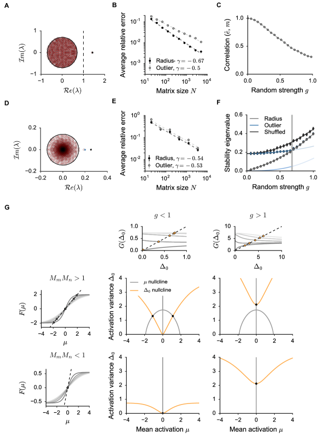
Figure S1:

Figure S2: Dynamical Mean-Field description of rank-one networks whose right- and left-connectivity vectors overlap solely on the unitary direction ($\rho=0$, see Methods). Related to Figure 1.

(A-B-C) Eigenspectrum of the partially structured connectivity matrix $J_{ij}$, related to the stability matrix $S_{ij}$ of the homogeneous fixed points through: $S_{ij}=\phi^{\prime}(\bar{x})J_{ij}$. A. Eigenspectrum of $J_{ij}$ in the complex plane. Red dots: eigenspectrum of a single realization $J_{ij}$ of size $N=1000$. In black: theoretical prediction. Every matrix $J_{ij}$ consists of a sum of a random and of a fixed unit-rank structure. In the large $N$ limit, the spectrum of the full matrix is given by the sum of the eigenspectra of the two parts. The black circle has radius equal to the total random strength $g$, and the black star indicates the position of the non-zero eigenvalue of the rank-one structure $P_{ij}$. B. Mismatch between the statistics measured in finite-size networks ($x_{sim}$) and the theoretical prediction ($x_{th}$) as the network size $N$ is increased. The error is normalized: $|x_{sim}-x_{th}|/x_{th}$. Averages over 100 realizations. The error bars (as in every other figure, if not differently specified) correspond to the standard deviation of the mean. Dashed lines: power-law best fit ($y\propto N^{\gamma}$). The values of $\gamma$ are indicated in the legend. C. Pearson correlation coefficient between the connectivity eigenvector $m$ and the eigenvector $\hat{e}$ which corresponds to the outlier eigenvalue. Choice of the parameters: $\rho=0$, $M_{m}M_{n}=1.43$, $\Sigma_{m}=0.33$, $\Sigma_{n}=1$. In A and B, $g=0.7$.

(D-E-F) Analysis of the eigenspectrum of the linear stability matrix $S_{ij}=\phi^{\prime}(\bar{x})J_{ij}$ for heterogeneous stationary solutions. D. Eigenspectrum of $S_{ij}$ in the complex plane. Red dots: eigenspectrum of a single, finite-size realization of $S_{ij}$, $N=2500$. The radius of the black circle corresponds to the theoretical prediction $r=g\sqrt{\langle[\phi_{i}^{\prime 2}]\rangle}$. The black star indicates the position of the non-zero eigenvalue of the rank-one structure ${m_{i}\phi^{\prime}(x_{j}^{0})n_{j}}/{N}$, which deviates significantly from the position of the outlier eigenvalue. We thus address the problem of evaluating the position of the outlier eigenvalue through a mean-field stability analysis (Eq. 71), the prediction of which is indicated by the blue star. E. Mismatch between the results from simulations and mean-field predictions for the radius and the outlier position. The error is measured as an average over $N_{tr}=30$ finite size matrices, and decays as the system size is increased. Details as in B. F. Radius and outlier of the stability eigenspectrum for increasing random strength values. The dots indicate the results of numerical simulations of networks with $N=2500$ units, averaged over $N_{tr}=30$ realizations of the random and structured connectivities. In grey: radius of the compact bulk (continuous line: mean-field prediction $r$). In blue: position of the outlier eigenvalue (continuous dark and light lines: first and second eigenvalue of matrix $\mathcal{M}$ given in Eq. 71). In black: position of the outlier when $\chi_{ij}$ is shuffled (continuous line: mean-field prediction for the outlier of the structured part ${m_{i}\phi^{\prime}(x_{j}^{0})n_{j}}/{N}$). Choice of the parameters: $\rho=0$, $M_{m}M_{n}=2.2$, $\Sigma_{m}=0.4$, $\Sigma_{n}=1$. In D and E, $g=0.5$.

(G) Graphical analysis of stationary solutions. Large figures: nullcline plots for the population-averaged DMF equations in Eq. 83. Black dots indicate the solutions that are stable with respect to the outlier eigenvalue. Four set of parameters (two values for $M_{m}M_{n}$, two for $g$) have been selected. Note that the shapes of the $\mu$ and the $\Delta_{0}$ nullcline depend only on the structure strength $M_{m}M_{n}$ and the disorder strength $g$. For the figures in the first (resp. second) row, the structure strength $M_{m}M_{n}=0.55$ (resp. $M_{m}M_{n}=2.0$) is weak (resp. strong). For the figures in the first (resp. second) column: the random strength $g=0.7$ (resp  $g=2.0$) is weak (resp. strong). Note that the stationary states at large $g$ values (right column) are always unstable with respect to the continuous component of their stability eigenspectra (Fig. 1 C-D). The small side figures associated to every row and column show how the $\mu$ (for the rows) and $\Delta_{0}$ (for the columns) nullclines have been built. We solve $\mu=F(\mu)$ (resp. $\Delta_{0}=G(\Delta_{0})$) for different initial values of $\Delta_{0}$ (resp. $\mu$). Different initial conditions are displayed in gray scale. Dark grey refers to $\Delta_{0}=0$ (resp. $\mu=0$). The dots indicate the solutions for different initial values, which together generate the nullcline curves. Choice of the parameters: $\Sigma_{m}=1$.

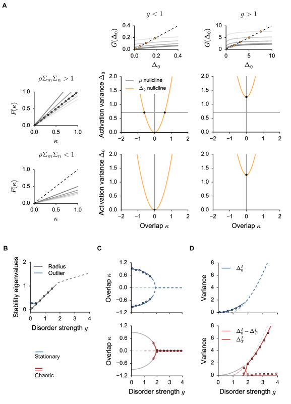
Figure S3:

Figure S4: Dynamical Mean-Field description of rank-one networks whose right- and left-connectivity vectors overlap onto an arbitrary direction $y$ ($M_{m}=M_{n}=0$, $\rho\neq 0$, see Methods). Related to Figure 1.

(A) Graphical analysis of stationary solutions. Large figures: nullcline plots for the population-averaged DMF equations in Eq. 89. Black dots indicate the solutions that are stable with respect to the outlier eigenvalue. Four set of parameters (two values for $\rho\Sigma_{m}\Sigma_{n}$, two for $g$) have been selected. Note that the shapes of the $\kappa$ and the $\Delta_{0}$ nullcline depend only on the structure strength $\rho\Sigma_{m}\Sigma_{n}$ and the disorder strength $g$. For the figures in the first (resp. second) row, the structure strength $\rho\Sigma_{m}\Sigma_{n}$ (resp. $\rho\Sigma_{m}\Sigma_{n}$) is weak (resp. strong). For the figures in the first (resp. second) column: the random strength $g=0.5$ (resp. $g=1.7$) is weak (resp. strong). Note that the stationary states at large $g$ values (right column) are always unstable with respect to the continuous circular component of their stability eigenspectra (see B-C-D). The small figures associated to every row and column show how the $\kappa$ (for the rows) and $\Delta_{0}$ (for the columns) nullclines have been built. We solve $\kappa=F(\kappa)$ (resp. $\Delta_{0}=G(\Delta_{0})$) for different initial values of $\Delta_{0}$ (resp. $\kappa$). Different initial conditions are displayed in gray scale. Dark grey refers to $\Delta_{0}=0$ (resp. $\kappa=0$). The dots indicate the solutions for different initial values, which together generate the nullcline curves.

(B-C-D) Bifurcation diagram of the activity statistics as the random strength $g$ is increased. Details as in Fig. 1 C-D. B. Stability eigenspectrum of stationary solutions, mean-field prediction for the radius of the compact part and the outlier position. C. Overlap $\kappa=\langle n_{i}[\phi_{i}]\rangle$. D. Individual second order statistics. The DMF solutions are displayed as continuous (resp. dashed) lines if they correspond to a stable (resp. unstable) state. In C-D, top panels display statistics for stationary solutions and bottom panels display statistics for chaotic solutions. Dots: we measured activity statistics in finite-size networks, starting from globally positive and negative initial conditions. Activity is integrated up to $T=400$. $N=3500$, average over 8 different network realizations. Choice of the parameters: $\Sigma_{m}=\Sigma_{n}=1.5$, $\rho=2.0/\Sigma_{m}\Sigma_{n}$.

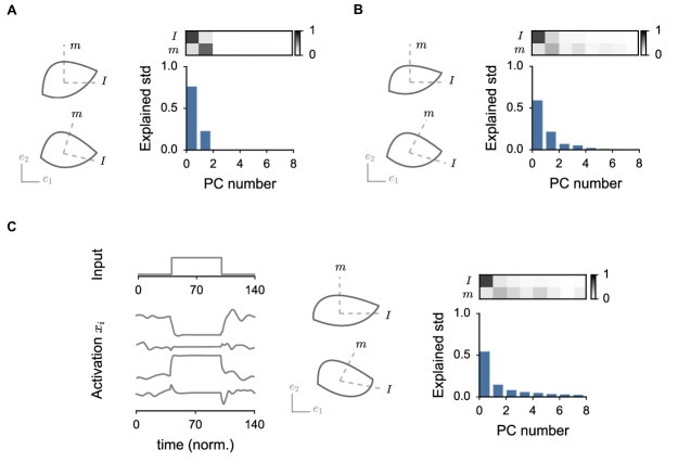
Figure S5:

Figure S6: Two-dimensional dynamics in networks with unit-rank structure and external inputs. Related to Figure 2.

We consider a unit-rank network as in Fig. 2 B-C. The connectivity vectors $m$ and $n$ are orthogonal, but the external input vector contains a component along $n$, whose strength (quantified by $\Sigma_{nI}$, see Methods) undergoes a step increase from $0.2$ to $2.0$. We simulate data from networks of size $N=3500$. We analyze the dimensionality of the dynamics by comparing the relevant low-dimensional trajectory predicted by the mean-field theory with the strongest modes extracted through dimensionality reduction (Principal Component analysis, see Methods). A. Analysis for a purely structured network ($g=0$). Left top: the mean-field theory predicts that the low-dimensional network dynamics $x=\{x_{i}\}$ lies in the plane defined by the right-connectivity vector $m$ and the external input $I$. We thus projected the high-dimensional population activity (dark grey trajectory) on this plane. Left bottom: we projected the network dynamics (continuous), along with the two vectors $m$ and $I$ (dashed), on the plane defined by the first two PC axis $e_{1}$ and $e_{2}$. Right top: Pearson correlation coefficient between vectors $m$ and $I$ and the first eight PC. Right bottom: strength of the first eight PC, measured as the fraction of the standard deviation of activity that they explain (see Methods). Note that when the network connectivity is fully structured ($g=0$) as in this case, activity is exactly two-dimensional. The first two PC axis span the $m-I$ plane, but they define a rotated set of basis vectors. B. Analysis for a network which includes a random term in the connectivity matrix ($g=0.8$). While in Fig. 2 we performed the PC decomposition on trial-averaged data ($N_{tr}=20$), here we considered a single trial, defined as a single realization of the random connectivity matrix. Details as in A. Note that the random component of the connectivity adds noisy contributions in a continuum of PC directions, whose strength depends on the value of $g$ with respect to the amplitude of input and connectivity vectors, and becomes weaker and weaker when averaging with respect to different realizations of $\chi_{ij}$. When $g>0$, vectors $m$ and $I$ are not fully contained in the $e_{1}-e_{2}$ plane, so their projections on the PC plane are not orthogonal. C. Analysis for a network which includes a strong random term in the connectivity matrix ($g=1.8$), such that spontaneous activity is chaotic. In the left-most column, similarly to Fig. 2, we plot the time trajectories of four randomly selected units. The center and the right columns are as in A and B, with PCA performed on trial-averaged activity ($N_{tr}=20$). The scale of the projections panels is here set arbitrarily.

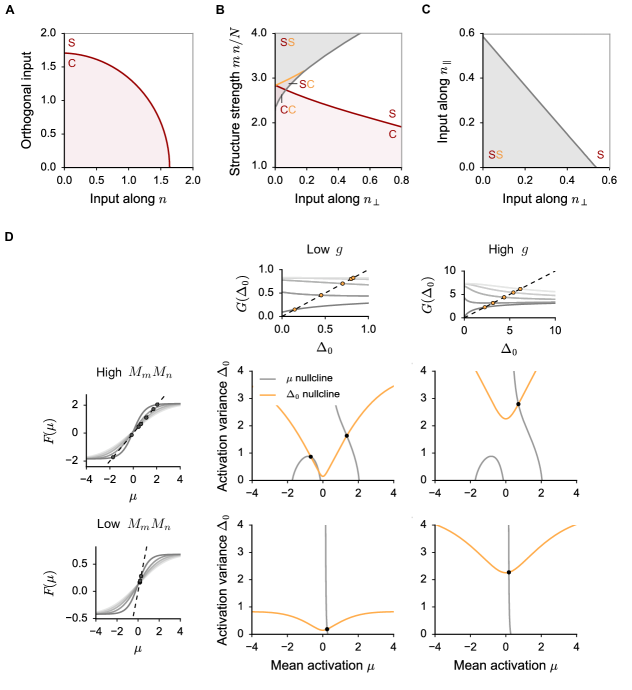
Figure S7:

Figure S8: Dynamical Mean-Field description of input-driven dynamics for rank-one networks whose right- and left-connectivity vectors overlap solely on the unitary direction ($\rho=0$, see Methods). Related to Figure 2.

(A-B-C) Dynamical regimes of the network activity as function of the structure connectivity strength $m^{T}n/N$, the random strength $g$ and the input strength. Grey shaded areas indicate the parameter regions where the network activity is bistable. Red shaded areas indicate the phase space regions where network dynamics are chaotic. When two stable solutions exist, the yellow and the red letter indicate whether each of them is stationary (S) or chaotic (C). Note that stationary and chaotic dynamics can coexist (SC region). In A, as in Fig. 2 D center, the two connectivity vectors $m$ and $n$ are orthogonal. We varied the external input strength by increasing the amplitude of the component along $n$ (quantified by $\Sigma_{nI}$, see Methods) and of the orthogonal one (quantified by $\Sigma_{\perp}$). Note that inputs along both directions contribute to suppressing the amplitude of chaotic fluctuations. In B, as in Fig. 2 D right, the two connectivity vectors $m$ and $n$ are not orthogonal, but they share an overlap component along the unitary direction. We varied the structure strength (quantified by $M_{m}M_{n}$) and the strength of the input along the direction of $n$ that is perpendicular to the structure overlap, $n_{\perp}$ (again quantified by $\Sigma_{nI}$). Similarly to Fig. 1, strong structure overlaps can lead to the appearance of two bistable solutions. In presence of non trivial external inputs, however, such solutions are not symmetric, and can loose stability on different parameter boundaries. In particular, we observe that external inputs tend to suppress bistable regimes, by favouring one solution over the other. In C, finally, the network configuration is similar to B, but we consider external inputs which include a second component along the direction of $n$ that is shared with $m$, $n_{\parallel}$ (quantified by $M_{I}$). We observe that both input directions play similar roles in reducing the extent of the bistable regime. Choice of parameters: $g=2.2$, $\Sigma_{m}=\Sigma_{n}=1.0$, $\Sigma_{mI}=0$.

(D) Graphical analysis of stationary solutions. In this example, the external input vector overlaps with $n$ on the unitary overlap direction $n_{\parallel}$ ($M_{I}=0.13$), and includes orthogonal components quantified by $\Sigma_{I}=0.3$. Large figures: nullcline plots for the stationary form of the population-averaged DMF equations in Eq. 98. Black dots indicate the solutions that are stable with respect to the outlier eigenvalue. Four set of parameters (two values for $M_{m}M_{n}$, two for $g$) have been selected. Note that the shape of the $\mu$ and the $\Delta_{0}$ nullcline depends only, respectively, on the structure strength $M_{m}M_{n}$ and the disorder $g$ together with the input statistics. For the figures in the first (resp. second) row, the structure strength $M_{m}M_{n}=0.55$ (resp. $M_{m}M_{n}=2.0$) is weak (resp. strong). For the figures in the first (resp. second) column: the random strength $g=0.7$ (resp. $g=2.0$) is weak (resp. strong). The small figures associated to every row and column show how the $\mu$ (for the rows) and $\Delta_{0}$ (for the columns) nullclines have been built. We solve $\mu=F(\mu)$ (resp. $\Delta_{0}=G(\Delta_{0})$) for different initial values of $\Delta_{0}$ (resp. $\mu$). Different initial conditions are displayed in gray scale. Dark grey refers to $\Delta_{0}=0$ (resp. $\mu=0$). The dots indicate the solutions for different initial values, which together generate the nullcline curves. Choice of the parameters: $\Sigma_{m}=1$.

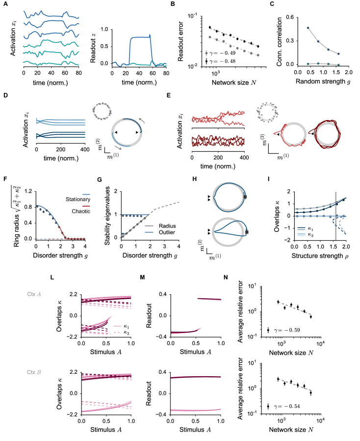
Figure S9:

Figure S10: Dynamical Mean-Field description of low-rank networks designed for solving computational tasks. Related to Figures 3, 5 and 6.

(A-B-C) Rank-one networks can robustly perform computations also when their dynamics is chaotic due to large random connectivities. Here, we show an example from the Go-Nogo task (Fig. 3). We focus on large random strength values ($g=2.5$), so that spontaneous network dynamics is chaotic. A. Left: response of three randomly selected units to the Go pattern $I^{A}$ (top, blue) and to the Nogo pattern $I^{B}$ (bottom, green). Right: time trace of the readout $z(t)$ for the Go (blue) and the Nogo (green) stimulus. B. Absolute, normalized distance between the theoretical prediction and the value of the readout $z$ obtained from finite-size realizations. As expected, the magnitude of the average normalized error decays with the network size as $\sim 1/\sqrt{N}$. In grey: $g=0.8$, in black: $g=2.5$. Averages over 200 network realizations. Details as in Fig. S1 B. C. As in Fig. 3 F, we consider pairs of units and we compute the correlation coefficient between their weights onto the first PC axis and their average reciprocal connectivity strength. The PC axis is computed separately for data corresponding to Go (blue) or the Nogo (green) trials. The correlation coefficient for the Go trials decreases with the amplitude of the random connectivity, although the error in the readout is only weakly affected (panel B.). For every entry of the connectivity matrix $J_{ij}$, indeed, the random part $g\chi_{ij}$ has larger amplitude then the structured one $P_{ij}$. As a consequence, the random noise can hide a fraction of the strong correlations existing between the PC weights and the rank-one connectivity $P_{ij}$. Note that the absolute value of the correlation coefficient depends on the variance of the rank-one connectivity. Finally, the correlation coefficient increases as the connectivity gets averaged on more and more realizations of the random part. Choice of the parameters as in Fig. 3.

(D-E-F-G-H-I) Ring attractor from rank-two connectivity structures with connectivity vectors characterized by strong internal overlaps (see Methods). D. Sample of activity from a finite-size realization ($N=4000$) of the rank-two network. Activity is initialized in two different initial conditions (light and dark blue), indicated by the small arrows. Left: time traces of the activation variables for three randomly selected network units. Note the long time range on the $x$ axis. Right: population activation $x=\{x_{i}\}$ projected on the plane spanned by the right vectors $m^{(1)}$ and $m^{(2)}$. The ring attractor predicted by the mean-field theory is displayed in light gray. The strength of the disorder is $g=0.5$, so that the network is in a stationary regime. In the small inset, we reproduce the theoretical prediction together with the final state of additional $N_{tr}=20$ networks realizations, that are displayed as grey dots. E. Sample of activity for two finite-size realizations ($N=4000$) of the structured connectivity matrix (dark and light red). Details as in D. The strength of random connections is $g=2.1$, so that the network is in a chaotic regime. Chaotic fluctuations can occur together with a slow exploration of the ring (dark red). If two specific states on the ring appear to be more stable, chaotic fluctuations can induce jumps between the two of them (light red). F-G. Mean-field characterization of the ring structure: radius of the ring attractor and stability eigenvalues. Details as in Fig. 1. Dots: numerical results from finite-size ($N=4000$) networks, averaged over 6 realizations of the connectivity matrix. H-I. Input patterns which correlate with the left vector $n^{(1)}$ reduce the ring attractor to a single stable state. Activity is thus projected in the direction spanned by the right vector $m^{(1)}$. In H, we show the input response for two finite-size networks. The grey ring displays the mean-field solution in absence of external inputs ($g=0.5$, as in D). In the top panel, the input is weak ($\Sigma_{I}=0.2$, see Methods). The transient dynamics as well as the equilibrium state lie close to the ring structure. In the bottom panel, the input is strong ($\Sigma_{I}=0.6$), and the ring structure is not anymore clearly apparent. In I, we plot the values of the overlaps $\kappa_{1}$ (blue) and $\kappa_{2}$ (azure) as a function of the structure strength parameter $\rho$, for fixed input strength. Stable solutions are plotted as continuous lines, unstable ones as dashed. Solid (resp. transparent) lines refer to weak (resp. strong) external inputs: $\Sigma_{I}=0.2$ (resp. 0.6). The vertical gray line indicate the value of $\rho$ that has been used in H. Dots: numerical results as in F-G. Choice of the parameters (see Methods): $\Sigma=2.0$, $\rho_{1}=\rho_{2}=1.6$.

(L-M-N) Rank-two structures for implementing non-linear stimuli detection in a context-dependent fashion (Fig. 6): theoretical mean-field predictions. L. Values of the first-order statistics $\kappa_{1}$ (continuous) and $\kappa_{2}$ (dashed) as a function of the overlap strength along the stimulus $I^{A}$. Results are shown for four increasing values of the overlap strength along the second stimulus $I_{B}$. Top (resp. bottom): the contextual gating inputs are such that a response to $I^{A}$ (resp. $I^{B}$) is selected. M. Readout value, built by summing the values of $\kappa_{1}$ and $\kappa_{2}$ (Eq. 158). Note that although $\kappa_{1}$ and $\kappa_{2}$ vary with input strength, on each branch their sum is approximately constant. Details as in L. N. Average normalized error between the DMF predictions and the simulated readout, in the two gating conditions as a function of the network size $N$. Average over 60 network realizations, details as in Fig. S1 B. Parameters as in Fig. 6.

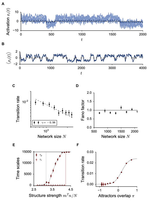
Figure S11:

Figure S12: Dynamics of unit-rank networks of finite-size are characterized by two distinct time-scales. Related to Figure 1.

In Fig. 1 we have shown that, when the structure strength is large, the DMF theory predicts the existence of two bistable states, which can display chaotic activity. For those states, the population-averaged statistics of the activation variable $x_{i}$ are stationary. In the chaotic regime, indeed, irregular temporal fluctuations are decorrelated from one unit to the other, so that the central limit theorem applies at every time step, and the network statistics are constant in time. In finite-size networks, however, the network statistics are not stationary: their dynamics display instead two different time-scales. The instantaneous population-averaged activity undergoes small fluctuations of amplitude $\mathcal{O}(1/\sqrt{N})$, whose time-scale is given by the relaxation decay of chaotic activity. Because of bistability, furthermore, the first-order statistics displays also sharp transitions from positive to negative values and viceversa, which are made possible by the self-sustained temporal fluctuations. In the following, we focus on rank-one structures where the overlap direction is defined along the unitary vector. As a consequence, the relevant first-order statistics is simply the population-average of the activation vector $\mu$ (see Methods). A. Sample from a finite-size network: activation time traces for randomly chosen units displaying attractors jumps. Dashed blue line: time-dependent population average. B. Time-dependent population average in a longer trial. C-D. We consider transition events as point processes, and we measure the average transition rate. We arbitrarily define a transition point as the time step at which the population-averaged activation crosses zero (grey points in B). In C, we show that the transition rate decays to zero as the network size $N$ is increased. Details as in Fig. S2 B. Note that the transition rate depends on the amplitude of finite-size fluctuations measured with respect to the average phase space distance between the two attractors. As a consequence, the transition rate depends on the architecture parameters and on the network size, but also varies strongly from one realization of the connectivity matrix to the other. D. Fano factor of the point process for different values of the network size $N$, which noisily oscillates around 1. For every realization of the network, the jumps count is measured in different windows of the total integration time $T=15.000$. The Fano factor is measured for every realization and then averaged over $N_{tr}=30$ different networks. E-F. Analysis of the two time-scales displayed by the network dynamics. The first time-scale is measured as the relaxation time constant $\tau_{r}$, which can be derived within the DMF framework by computing the time decay of the full auto-correlation function $\Delta(\tau)$. The persistence time scale, indicated by $\tau_{p}$, coincides instead with the average time interval which separates two attractors transitions. In E, we show that both time scales depend on the network architecture parameters. Here, we fix the random strength $g=3$ and we increase the structure strength. When the structure is weak (left), the network is in the classical homogeneous chaotic state. The persistence time scale coincides here with the relaxation time constant of chaotic fluctuations. When the structured and the random components have comparable strengths, instead, two heterogeneous chaotic phases co-exist (center). In this regime, the average persistence time increases monotonically with the structure strength, and reaches arbitrarily large values. Note that the relaxation time undergoes a very slow increase before sharply diverging at the boundary with stationary states, but the increase takes place on a much smaller scale. Finally, if the structure is too strong (right), the two bistable states become stationary. In this region, $\tau_{r}$ is formally infinite, while $\tau_{p}$ coincides with the total duration of our simulations. Pink continuous line: DMF prediction, measured as the full width half maximum of the auto-correlation function $\Delta(\tau)$. Pink dots: a rough estimate of $\tau_{r}$ from finite size networks is obtained by rectifying the population average signal and we computing the full width half maximum of its auto-correlation function. F. We compare the average transition rate with the average overlap between the two attractors in the phase space. For every unit, the typical overlap between its positive and its negative trajectories is given by $\pi_{i}=2(-\mu-\sqrt{\Delta_{\infty}}z+\sqrt{\Delta_{0}-\Delta_{\infty}})$. We average across the population, yielding: $\pi=2(-\mu+\sqrt{\Delta_{0}-\Delta_{\infty}})$. We then normalize $\pi$ through dividing by its value in the unstructured chaotic regimes ($2\Delta_{0}$). When positive, $\pi$ returns an overlap; when negative, it measures a distance between the two orbits. For every set of the architecture parameters, the theoretical expected value of the overlap can be computed within the DMF framework. We show that, in finite-size networks, the transition probability between the two chaotic attractors monotonically increases with the attractors overlap in the phase space. In the figure, the points returned by simulations are fitted with an error function of which we evaluate numerically the amplitude, the offsets and the gain: $f(x)=p_{0}+p_{1}\>\mathrm{erf}(p_{2}(x-p_{3}))$. Choice of the parameters: $\rho=0$, $g=3.0$, $\Sigma_{m}=0$.

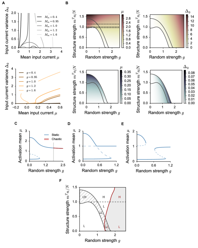
Figure S13:

Figure S14: Dynamics of unit-rank networks with positively-defined activation functions. Related to Figure 1.

In the main text, we performed our analysis of low-rank networks by adopting a completely symmetric network model, whose input-free solutions are invariant under the sign transformation $x_{i}(t)\rightarrow-x_{i}(t)$. Such symmetry is broken when a more biologically-plausible, positively-defined activation function $\phi(x)$ is adopted. Here, we investigate the effect of changing the transfer function to: $\phi(x)=1+\tanh(c(x-\gamma))$. Note that adding a shift $\gamma$ is equivalent to including an external and constant negative input. The parameter $c$, instead, rescales the slope of $\phi(x)$ at the inflection point. For simplicity, we fix $\gamma=1$ and $c=1.5$. We furthermore restrict the analysis to the case of unit-rank structures whose right- and left-connectivity vectors solely overlap on the unitary direction ($\rho=0$, see Methods). The Dynamical Mean Field (DMF) sets of equations were derived for an arbitrary activation function, so they can directly be adapted to the present scenario. A. We start by graphically analysing the stationary solutions (Eq. 83), and we plot the two nullclines of the system for different values of the architecture parameters. The top panel displays the $\mu$ nullclines for different $M_{m}M_{n}$ values. At $M_{m}M_{n}=1$, the unstable branch coincides with $\mu=1$, and the stable ones are symmetric. Around $M_{m}M_{n}=1$, the perfect pitchfork is broken in one or the other direction, generating a first stable continuous branch and a second one, where one unstable and one stable solution merge at low or high firing rate. For extremely low (resp. high) $M_{m}M_{n}$ values, finally, there’s just one nullcline at low (resp. high) $\mu$ values. The $\Delta_{0}$ nullcline (bottom panel) displays a more complex behaviour compared to the symmetric $\phi(x)=\tanh(x)$ case. When $g$ is sufficiently large, indeed, it can become a non-monotonic function of the mean input $\mu$, transforming into a S-shaped nullcline. As it is shown in the following, this more complex shape is able to induce bistable activity even when the $\mu$ nullcline is reduced to a single continuous branch. This situation is reminiscent of the fluctuations driven bistable regime in [Renart et al, 2007]. B. Stationary stable solutions plotted as color maps on the parameter space defined by the random and the structure strengths. The mean-field system admits two classes of stable solutions. The first one, illustrated in the top row, takes large mean and variance values. It suddenly disappears on the leftmost grey boundary of the plot, in a parameter region which co-exists with the second solution. The second solution, plotted in the bottom row, takes typically small values of $\mu$ and $\Delta_{0}$, and disappears on the right-most boundary with a first-order transition as well. C-D-E. In order to dissect more systematically the nature of those solutions, we fix the value of the structure strength (dashed lines in in B), and we gradually increase the random strength $g$. In C, we fix the structure strength to high values: $M_{m}M_{n}=1.2$. The bifurcation pattern occurring in this case resembles what we observed in the original case with $\phi(x)=\tanh(x)$. At low values of $g$, two stable fixed points are built, respectively, on the high and on the low branches of the $\mu$ nullcline. For that reason, we call this state LH (cfr with F). When the random connectivity is too strong, the low firing rate fixed point annihilates, and only one high firing solution survives (H state). In D, $M_{m}M_{n}$ is exactly equal to unity. At small $g$ values, similarly to the previous case, network activity is bistable and admits one L and one H stationary state. As $g$ increases, the $\Delta_{0}$ intersect the high firing rate branch at smaller and smaller values of $\mu$. Finally, the H state is lost, and the second stable fixed point is realized on the intermediate branch at $\mu=1$. This bistable state is thus formally a LI state. Finally, at large $g$ values, the two intersections on the low rate branch collapse together and disappear. Bistability is lost and only one intermediate (I) state exists. In E, we consider slightly smaller values of $M_{m}M_{n}$. A classical LH state exists at small $g$ values, the bistable state at large random strengths involves two stable solutions which originate both a low firing rates (LL state). The two states strongly differ in the value of their variance. When $g$ is sufficiently large, one unique low firing rate, high variance state (L) survives. F. The different activity states are finally sketched in the phase diagram. Note that I states separate the phase diagram in F in two macro areas: below the dashed line, every stationary and chaotic solution is built on the same low firing rate branch of the $\mu$ nullcline, and is thus formally a L state. Finally, the exact shape of the phase diagram depends on the value of the parameters $c$ and $\gamma$. Choice of the parameters: $\rho=0$, $\Sigma_{m}=0$.

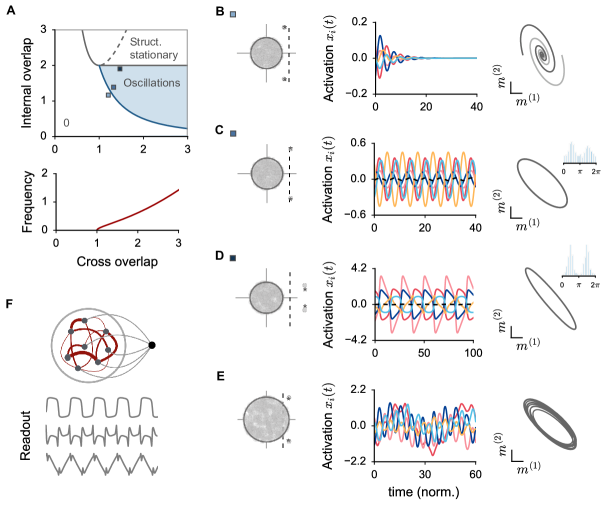
Figure S15:

Figure S16: Oscillatory activity from rank-two structures that include a cross overlap between left- and right-connectivity vectors.

A. Top: phase diagram for the rank-two structure with negative cross-overlap (see Methods). For different values of the internal and the cross overlaps, the trivial fixed point can lose stability and give rise to oscillatory or stationary structured activity. The Hopf bifurcation is indicated in blue, the instability to stationary activity in grey. The light-blue parameter region corresponds to sustained non-linear oscillations. Bottom: frequency of oscillations along the Hopf bifurcation boundary, in units defined by the implicit time scale of the network dynamics. B-C-D-E. Samples of activity for different connectivity parameters. From left to right: stability eigenspectrum of the trivial fixed point (theory and simulations), sample of activation trajectories (the population average is indicated in dashed black), and population dynamics obtained by projecting the population activation $x$ on the right-connectivity vectors $m^{(1)}$ and $m^{(2)}$. The parameters that have been used for every sample are indicated in A. B: Oscillatory transients in the fixed point regime. C: Stable oscillations above the Hopf instability. The elongated shape of the closed trajectory on the $m^{(1)}-m^{(2)}$ plane is inherited by the phase distribution across the population, and can be tuned by slightly modifying the parameters of the rank-two structure (see Methods). D: Highly non-linear oscillations close to the boundary with bistable activity. E: Oscillatory activity at high $g$ values ($g=1.35$), where dynamics include a chaotic component. F. When oscillations are strongly non-linear, their spectrum includes a large variety of frequencies that can be used to reproduce highly non-linear periodic patterns. We designed three random readout vectors and we linearly decoded activity from the dynamical regime in D to generate periodic non-linear outputs, which are displayed in grey.

References

- Ahmadian et al. (2015) Ahmadian, Y., Fumarola, F. and Miller, K. D. (2015). Properties of networks with partially structured and partially random connectivity. Phys. Rev. E, 91:012820.
- Aljadeff et al. (2015b) Aljadeff, J., Stern, M. and Sharpee, T. (2015b). Transition to chaos in random networks with cell-type-specific connectivity. Phys. Rev. Lett., 114:088101.
- Amit and Brunel (1997) Amit, D. J. and Brunel, N. (1997). Model of global spontaneous activity and local structured activity during delay periods in the cerebral cortex. Cereb. Cortex, 7(3):237–252.
- Amit et al. (1985) Amit, D. J., Gutfreund, H. and Sompolinsky, H. (1985). Storing infinite numbers of patterns in a spin-glass model of neural networks. Phys. Rev. Lett., 55:1530–1533.
- Barak (2017) Barak, O. (2017). Recurrent neural networks as versatile tools of neuroscience research. Curr. Opin. Neurobiol., 46:1 – 6.
- Ben-Yishai et al. (1995) Ben-Yishai, R., Bar-Or, R. L. and Sompolinsky, H. (1995). Theory of orientation tuning in visual cortex. Proc. Natl. Acad. Sci. USA, 92(9):3844–3848.
- Boerlin et al. (2013) Boerlin, M., Machens, C. K. and Deneve, S. (2013). Predictive coding of dynamical variables in balanced spiking networks. PLOS Comput. Biol., 9(11):1–16.
- Brunel (2000) Brunel, N. (2000). Dynamics of sparsely connected networks of excitatory and inhibitory spiking neurons. J. Comput. Neurosci., 8(3):183–208.
- Churchland and al. (2010) Churchland, M. M. and al. (2010). Stimulus onset quenches neural variability: a widespread cortical phenomenon. Nat. Neurosci., 13(3):369–378.
- Churchland and Shenoy (2007) Churchland, M. M. and Shenoy, K. V. (2007). Temporal complexity and heterogeneity of single-neuron activity in premotor and motor cortex. J. Neurophysiol., 97(6):4235–4257.
- Cunningham and Yu (2014) Cunningham, J. P. and Yu, B. M. (2014). Dimensionality reduction for large-scale neural recordings. Nat. Neurosci., 17(11):1500–1509.
- Doiron and Litwin-Kumar (2014) Doiron, B. and Litwin-Kumar, A. (2014). Balanced neural architecture and the idling brain. Front. Comput. Neurosci., 8:56.
- Eliasmith and Anderson (2004) Eliasmith, C. and Anderson, C. (2004). Neural Engineering - Computation, Representation, and Dynamics in Neurobiological Systems. MIT press.
- Fusi et al. (2016) Fusi, S. Miller, E. K. and Rigotti, M. (2016). Why neurons mix: high dimensionality for higher cognition. Curr. Opin. Neurobiol., 37:66 – 74.
- Gao and Ganguli (2015) Gao, P. and Ganguli, S. (2015). On simplicity and complexity in the brave new world of large-scale neuroscience. Curr. Opin. Neurobiol., 32:148–55.
- Girko (1985) Girko, V. L. (1985). Circular law. Theory Probab. Appl., 29(4):694–706.
- Harish and Hansel (2015) Harish, O. and Hansel, D. (2015). Asynchronous rate chaos in spiking neuronal circuits. PLOS Comput. Biol., 11:1–38.
- Harris and Mrsic-Flogel (2013) Harris, K. D. and Mrsic-Flogel, T. D. (2013). Cortical connectivity and sensory coding. Nature, 503(7474):51–58.
- Hopfield (1982) Hopfield, J. J. (1982). Neural networks and physical systems with emergent collective computational abilities. Proc. Natl. Acad. Sci. USA, 79(8):2554–2558.
- Jaeger and Haas (2004) Jaeger, H. and Haas, H. (2004). Harnessing nonlinearity: Predicting chaotic systems and saving energy in wireless communication. Science, 304(5667):78–80.
- Kadmon and Sompolinsky (2015) Kadmon, J. and Sompolinsky, H. (2015). Transition to chaos in random neuronal networks. Phys. Rev. X, 5:041030.
- Kanerva (2009) Kanerva, P. (2009). Hyperdimensional computing: An introduction to computing in distributed representation with high-dimensional random vectors. Cogn. Comput., 1(2):139–159.
- Ko et al. (2011) Ko, H., Hofer, S. B., Pichler, B., Buchanan, K. A., Sjostrom, P. J. and Mrsic-Flogel, T. D. (2011). Functional specificity of local synaptic connections in neocortical networks. Nature, 473(7345):87–91.
- Litwin-Kumar and Doiron (2012) Litwin-Kumar, A. and Doiron, B. (2012). Slow dynamics and high variability in balanced cortical networks with clustered connections. Nat. Neurosci., 15(11):1498–1505.
- Maass et al. (2007) Maass, W., Joshi, P. and Sontag, E. D. (2007). Computational aspects of feedback in neural circuits. PLOS Comput. Biol., 3(1):1–20.
- Machens et al. (2010) Machens, C. K., Romo, R. and Brody, C. D. (2010). Functional, but not anatomical, separation of “what” and “when” in prefrontal cortex. J. Neurosci., 30(1):350–360.
- Mante et al. (2013) Mante, V., Sussillo, D., Shenoy, K. V. and Newsome, W. T. (2013). Context-dependent computation by recurrent dynamics in prefrontal cortex. Nature, 503(7474):78–84.
- Markovsky (2012) Markovsky, I. (2012). Low Rank Approximation - Algorithms, Implementations, Applications. Springer.
- Martens and Sutskever (2011) Martens, J. and Sutskever, I. (2011). Learning recurrent neural networks with hessian-free optimization. In ICML, 1033–1040.
- Mastrogiuseppe and Ostojic (2017) Mastrogiuseppe, F. and Ostojic, S. (2017). Intrinsically-generated fluctuating activity in excitatory-inhibitory networks. PLOS Computat. Biol., 13(4):1–40.
- Newsome et al. (1989) Newsome, W., Britten, K. and Movshon, A. (1989). Neuronal correlates of a perceptual decision. Nature, 341.
- Ostojic (2014) Ostojic, S. (2014). Two types of asynchronous activity in networks of excitatory and inhibitory spiking neurons. Nat. Neurosci., 17(4):594–600.
- Pascanu et al. (2013) Pascanu, R., Mikolov, T. and Bengio, Y. (2013). On the difficulty of training recurrent neural networks. In ICML, III–1310–III–1318.
- Rajan and Abbott (2006) Rajan, K. and Abbott, L. F. (2006). Eigenvalue spectra of random matrices for neural networks. Phys. Rev. Lett., 97:188104.
- Rajan et al. (2010) Rajan, K., Abbott, L. F. and Sompolinsky, H. (2010). Stimulus-dependent suppression of chaos in recurrent neural networks. Phys. Rev. E, 82:011903.
- Remington et al. (2018) Remington, E. D., Narain, D., Hosseini, E. and Jazayeri, M. (2018). Flexible sensorimotor computations through rapid reconfiguration of cortical dynamics. Neuron, 98(5):1005–1019.
- Rigotti et al. (2010) Rigotti, M., Rubin, D., Wang, X.-J and Fusi, S. (2010). Internal representation of task rules by recurrent dynamics: The importance of the diversity of neural responses. Front. Comput. Neurosci., 4:24.
- Rigotti et al. (2013) Rigotti, M., Barak, O., Warden, M. R., Wang, X.-J., Daw, N. D., Miller, E. K. and Fusi, S. (2013). The importance of mixed selectivity in complex cognitive tasks. Nature, 497(7451):585–590.
- Rivkind and Barak (2017) Rivkind, A. and Barak, O. (2017). Local dynamics in trained recurrent neural networks. Phys. Rev. Lett., 118:258101.
- Roudi and Latham (2007) Roudi, Y. and Latham, P. E. (2007). A balanced memory network. PLOS Comput. Biol., 3(9):1–22.
- Saez et al. (2015) Saez, A., Rigotti, M., Ostojic, S., Fusi, S. and Salzman, C. D. (2015). Abstract context representations in primate amygdala and prefrontal cortex. Neuron, 87(4):869–881.
- Shadlen and Newsome (1998) Shadlen, M. N. and Newsome, W. T. (1998). The variable discharge of cortical neurons: Implications for connectivity, computation, and information coding. J. Neurosci., 18(10):3870–3896.
- Shiino and Fukai (1993) Shiino, M. and Fukai, T. (1993). Self-consistent signal-to-noise analysis of the statistical behavior of analog neural networks and enhancement of the storage capacity. Phys. Rev. E, 48:867–897.
- Sompolinsky et al. (1988) Sompolinsky, H., Crisanti, A. and Sommers, H. J. (1988). Chaos in random neural networks. Phys. Rev. Lett., 61:259–262.
- Sussillo (2014) Sussillo, S. (2014). Neural circuits as computational dynamical systems. Curr. Opin. Neurobiol., 25:156 – 163.
- Sussillo and Abbott (2009) Sussillo, D. and Abbott, L. F. (2009). Generating coherent patterns of activity from chaotic neural networks. Neuron, 63(4):544 – 557.
- Sussillo and Barak (2012) Sussillo, D. and Barak, O. (2012). Opening the black box: Low-dimensional dynamics in high-dimensional recurrent neural networks. Neural Computat., 25(3):626–649.
- Tao (2013) Tao, T. (2013). Outliers in the spectrum of iid matrices with bounded rank perturbations. Probab. Theory Relat. Fields, 155(1):231–263.
- Thalmeier et al. (2016) Thalmeier, D., Uhlmann, M., Kappen, H. J. and Memmesheimer, R. (2016). Learning universal computations with spikes. PLOS Comput. Biol., 12(6):1–29.
- Tirozzi and Tsodyks (1991) Tirozzi, B. and Tsodyks, M. (1991). Chaos in highly diluted neural networks. EPL, 14(8):727.
- van Vreeswijk and Sompolinsky (1996) Van Vreeswijk, C. and Sompolinsky, H. (1996). Chaos in neuronal networks with balanced excitatory and inhibitory activity. Science, 274(5293):1724–1726.
- Wang et al. (2018) Wang, J., Narain, D., Hosseini E. and Jazayeri, M. (2018). Flexible timing by temporal scaling of cortical responses. Nat. Neurosci., 21:102—110.
- Wang (2002) Wang, X.-J. (2002). Probabilistic decision making by slow reverberation in cortical circuits. Neuron, 36(5):955–968.
- Williamson et al. (2016) Williamson, R. C., Cowley, B. R., Litwin-Kumar, A., Doiron, B., Kohn, A., Smith, M. A. and Yu, B. M. (2016). Scaling properties of dimensionality reduction for neural populations and network models. PLOS Comput. Biol., 12(12):1–27.