Enhanced precision bound of low-temperature quantum thermometry via dynamical control

Abstract

High-precision low-temperature thermometry is a challenge for experimental quantum physics and quantum sensing. Here we consider a thermometer modelled by a dynamically-controlled multilevel quantum probe in contact with a bath. Dynamical control in the form of periodic modulation of the energy-level spacings of the quantum probe can dramatically increase the maximum accuracy bound of low-temperatures estimation, by maximizing the relevant quantum Fisher information. As opposed to the diverging relative error bound at low temperatures in conventional quantum thermometry, periodic modulation of the probe allows for low-temperature thermometry with temperature-independent relative error bound. The proposed approach may find diverse applications related to precise probing of the temperature of many-body quantum systems in condensed matter and ultracold gases, as well as in different branches of quantum metrology beyond thermometry, for example in precise probing of different Hamiltonian parameters in many-body quantum critical systems.

Introduction

Precise probing of quantum systems is one of the keys to progress in diverse quantum technologies, including quantum metrology giovannetti11 ; braun18quantum ; kurizki15quantum , quantum information processing (QIP) hauke16 and quantum many-body manipulations strobel14 . The maximum amount of information obtained on a parameter of a quantum system is quantified by the quantum Fisher information (QFI), which depends on the extent to which the state of the system changes for an infinitesimal change in the estimated parameter paris09 ; caves94 ; correa15 ; zwick16 ; pasquale16 . Ways to increase the QFI, thereby increasing the precision bound of parameter estimation, are therefore recognized to be of immense importance gefen17 ; campbell18precision . Recent works have studied QFI for demonstrating the criticality of environmental (bath) information zwick16pra , QFI enhancement in the presence of strong coupling correa16 or by dynamically-controlled quantum probes zwick16 and the application of quantum thermal machines to quantum thermometry brunner17 .

Here we propose the synthesis of two concepts: quantum thermometry matteo12 ; correa15 ; correa16 ; brunner17 ; campbell18precision ; potts19fundamental ; hovhannisyan18measuring ; kiilerich18dynamical ; tuoriniemi16physics ; mehboudi19thermometry ; pasquale19quantum and temporally-periodic dynamical control that has been originally developed for decoherence suppression in QIP agarwal99 ; agarwal01 ; lidar04 ; zwick14 ; dieter16 . We show that such control can strongly increase the QFI that determines the precision-bound of temperature measurement, particularly at temperatures approaching absolute zero. Accordingly, such control may boost the ultralow-temperature precision bound of diverse thermometers, e.g. those based on Coulomb blockade meschke11comparison , metal - insulator - superconductor junctions raisanen18normal , kinetic inductance giazotto08ultrasensitive and novel hybrid superconductors giazotto15ferromagnetic . Alternatively, dynamical control may allow theese thermometers to accurately estimate a broad range of temperatures.

Results

Model: An example of our dynamically controlled quantum thermometer (DCQT) is a quantum wavepacket trapped in a potential and subjected to periodic modulation, while it is immersed in a thermal bath (Fig. 1a). Measurements of the wavepacket after it has reached a steady state provide information about the bath temperature.

Figure 1: Schematic realization of a quantum thermometer: (a) Schematic realization of a dynamically controlled quantum thermometer by a motional wavepacket of a state of a cavity, or an ion/atom trapped in an optical lattice potential. The frequency of the trap is periodically varied (black arrow) by modulating the length of the cavity, or the amplitudes of the lasers forming the trap. The wavepacket is in contact with a phonon bath, and relaxes to the corresponding thermal steady state at long times. (b) Same, for a spin-chain bath coupled to a two-level system whose resonant frequency is periodically modulated.

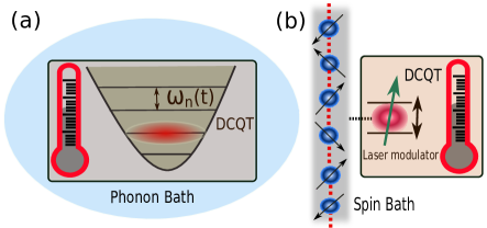
Another example of a DCQT is the internal state of either a two-level or a multilevel system coupled to a spin-chain bath ghosh11 ; ghosh12 . The level separation is periodically modulated by a control field (e.g. a field-induced alternating current Stark shift) and its level populations are finally read out by laser-induced fluorescence in the optical range (Fig. 1b). Many of the advanced thermometers correa16 ; brunner17 ; matteo12 ; meschke11comparison ; raisanen18normal ; giazotto08ultrasensitive ; giazotto15ferromagnetic may be adapted to such dynamically controlled operation.

The proposed DCQT is described by a Hamiltonian $H(t)$, subjected to a modulation with time period $\tau=2\pi/\Delta$:

$$\hat{H}(t+\tau) = \hat{H}(t)=\sum_{k}\hat{H}_{k}(t);$$

$$\hat{H}_{k}(t+\tau) = \hat{H}_{k}(t).$$ (1)

The DCQT is coupled to a bath through the interaction Hamiltonian of the form $\hat{H}_{I}=\sum_{k}\hat{H}_{Ik}=\sum_{k}\hat{S}_{k}\otimes\hat{B}_{k}$. Here $\hat{S}_{k}$ and $\hat{B}_{k}$ are, respectively, the $k$-th mode DCQT and bath operators. In cases where the $k$-th bath mode acts as a Markovian environment characterized by a mode-dependent unknown temperature $T_{k}$, the corresponding DCQT mode thermalizes to the temperature $T_{k}$ at long times, thus enabling us to perform mode-dependent thermometry. Alternatively, if the bath is thermal with an unknown temperature $T$, a single-mode DCQT suffices for bath temperature estimation.

Analysis: For simplicity, we restrict our analysis below to a thermal bath with temperature $T$, probed by an $\mathcal{N}$-level DCQT that is described by the Hamiltonian $\hat{H}(t)=\hbar\sum_{n=0}^{\mathcal{N}}\omega_{n}(t)|n\rangle\langle n|$ with energy spectrum $\omega_{n}(t)=n\omega(t)$ for real positive $\omega(t)$, and an interaction Hamiltonian $\hat{H}_{I}=\hat{S}\otimes\hat{B}$. Here $n$ denotes the level index, and we assume $\hat{S}$ to be a system operator belonging to a Lie algebra. For a two-level system, $\hat{S}\equiv\hat{\sigma}_{x}$, the $x$ Pauli operator, while for a harmonic oscillator, $\hat{S}\equiv\left(\hat{a}+\hat{a}^{\dagger}\right)$, where $\hat{a}$, $\hat{a}^{\dagger}$ denote the annihilation and creation operators, respectively. For a single-mode DCQT, we consider a generic, periodic, diagonal (frequency) modulation:

$$\omega(t) = \sum_{m^{\prime}=0}^{\infty}\Big{(}s(m^{\prime})\sin(m^{\prime}t\Delta)$$ (2)

$$+ c(m^{\prime})\cos(m^{\prime}t\Delta)\Big{)},$$

where $s(m^{\prime}),c(m^{\prime})$ are adjustable real constants, corresponding to the $m^{\prime}$-th frequency harmonic. One can extend this analysis to a multi-mode DCQT probing a multi-mode bath (see Methods).

Here we focus on controls with $\tau$ much smaller than the thermalization time of the system, such that one can adopt the secular approximation, thereby averaging out all rapidly oscillating terms and arriving at a time $t\gg\tau$ at the steady state $\hat{\rho}(t\to\infty)=\sum_{n=0}^{\mathcal{N}}\varrho_{n}|n\rangle\langle n|$ klimovsky13 ; alicki14 ; klimovsky15 . The level populations $\varrho_{n}$ are functions of the bath temperature $T$, the bath response (correlation) functions $G(\omega_{m})$ (see Methods) breuer02 ; yan18distinguishing at the $m$-th sideband frequency $\omega_{m}=\omega_{0}+m\Delta$, and the modulation-dependent $m$-th sideband weight $P_{m}\geq 0$ (see Methods and Apps. A - E). Here the sidebands $m=0,\pm 1,\pm 2,\ldots$ arise due to the periodic modulation, the mean frequency $\omega_{0}=\left(\int^{\tau}_{0}\omega(t)dt\right)/\tau$, and $P_{m}$’s satisfy the constraint $\sum_{m}P_{m}=1$ klimovsky13 ; alicki14 ; klimovsky15 . As can be expected in experiments, we impose an upper bound on the available resources for dynamical control, by considering only frequency modulations such that ${\rm max}\left[m^{\prime}\right]\Delta<\omega_{0}$. Unless otherwise stated, we take $\hbar$ and $k_{B}$ to be unity, and assume the bath response obeys the standard Kubo-Martin-Schwinger condition $G(-\omega)/G(\omega)={\rm exp}\left(-\omega/T\right)$ breuer02 .

We may infer the bath temperature $T$ from measurements of $\varrho_{n}$ of the thermometer: e.g., through measurement of the average phonon occupation number of a trapped-wavepacket probe (Fig. 1a) raymer04experimental , or the fluorescence of a two-level system probe (Fig. 1b). We can assess the effectiveness of our measuring scheme from the QFI as a function of the system and bath parameters. The relative error $\delta T/T$ is bounded by the minimal achievable error $\xi$, dictated by the Cramer-Rao bound for optimal positive-operator valued measure, which in this case are the level-population measurements. It obeys the relation paris09 ; brunelli11 ; zwick16

$$\frac{\delta T}{T}\geq\xi=\frac{1}{T\sqrt{\mathcal{M}\mathcal{H}}}.$$ (3)

Here $\mathcal{M}$ denotes the number of measurements, and $\mathcal{H}=-2\lim_{\epsilon\to 0}\partial^{2}F(\hat{\rho}(T,t),\hat{\rho}(T+\epsilon,t))/\partial\epsilon^{2}=\sum_{n=0}^{\mathcal{N}}|\partial\varrho_{n}/\partial T|^{2}/\varrho_{n}$ is the QFI at temperature $T$ caves94 ; pezze09 ; Kacprowicz10 ; correa15 , $F(\hat{\rho}_{1},\hat{\rho}_{2})={\rm Tr}\left[\sqrt{\sqrt{\hat{\rho}_{1}}\hat{\rho}_{2}\sqrt{\hat{\rho}_{1}}}\right]$ being the fidelity between $\hat{\rho}_{1}$ and $\hat{\rho}_{2}$.

The dynamics of the DCQT, and consequently also the resultant steady state, depends crucially on the factors $P_{m}G(\omega_{m})$; in general, a large $P_{m}G(\omega_{m})$ is beneficial for estimating temperatures $T\sim\omega_{m}$ (see below, Methods and Apps A - E Notes 1 - 5) klimovsky15 . Although we cannot control the bath correlation functions (spectral response) $G(\omega_{m})$, nevertheless for a given $G(\omega_{m})$, we can tailor the thermometry QFI to our advantage by judicious choices of the periodic control fields, and hence of the corresponding $P_{m}$’s and $\omega_{m}$’s. For example, a versatile thermometer which can measure a wide range of temperatures with high accuracy bound would require a modulation that corresponds to large QFI over a broad range of temperatures, in order to yield $\xi\ll 1$ for finite $\mathcal{M}$. The above scenario can be realized using modulations which give rise to multiple non-negligible $P_{m}$’s, or equivalently, large $P_{m}G(\omega_{m})$ over a broad range of frequencies. In particular, it is exemplified below using a sinusoidal modulation characterized by a single, or few frequencies. On the other hand, a different modulation would enable the same thermometer to measure temperatures with higher accuracy bound (or, equivalently, larger QFI), but at the expense of the changing of the temperature range over which the DCQT can measure accurately. This can for example be realized using periodic $\pi$-pulses, which give rise to only two sidebands, viz, non-negligible $P_{\pm 1}$ klimovsky13 .

Therefore, in contrast to thermometry in the absence of any control, DCQT gives us the possibility of tuning the range and accuracy bound of measurable temperatures. This necessitates an appropriate choice of control parameters ($\Delta,m^{\prime},s(m^{\prime}),c(m^{\prime})$) in Eq. (2) depending on the temperatures of interest.

Figure 2: Relative error bound and quantum Fisher information: Relative error bound $\xi$ for estimation of bath temperature $T$ (in units of $\omega_{0}$) by a harmonic oscillator dynamically controlled quantum thermometer (DCQT) under sinusoidal modulation for the following bath spectra: nearly flat bath spectrum (magenta solid curve), sub-Ohmic bath spectrum with $s=0.1,\omega_{c}=100$ (black dashed curve) and the same spectra in the absence of control (turquoise dotted curve). For low temperatures in the absence of control, $\xi\to\infty$, thus making it impossible to measure low temperatures as shown. In contrast, our dynamical control scheme reduces $\xi$ to finite values at low temperatures, for nearly flat, as well as sub-Ohmic bath spectra, thus showing the advantage of DCQT. Inset: Quantum Fisher Information ($\mathcal{H}$) as a function of temperature $T$ (in units of $\omega_{0}$) for DCQT under sinusoidal modulation and in the absence of control, for the bath spectra in the main figure (same curve colors). DCQT increases the quantum Fisher information significantly at lower temperatures, giving rise to a peak at $T\approx T_{-1}$ (magenta dot), in addition to the peak at $T\approx T_{0}$ (turquoise dot). Here the modulation amplitude $\mu=0.2,\omega_{0}=1,\Delta=0.9$ (see Eq. (6)), $m=0,\pm 1,\pm 2,\pm 3$ and the number of measurements $\mathcal{M}=1$. The thermalization time $\sim\gamma^{-1}$ is assumed to be long enough such that the secular approximation is valid.

Harmonic-oscillator DCQT for sub-Ohmic baths: As a generic example of DCQT, we consider the probe to be a periodically modulated harmonic oscillator. The interaction Hamiltonian is $\hat{H}_{I}=\left(\hat{a}+\hat{a}^{\dagger}\right)\otimes\hat{B}$, where $\hat{a}$ ($\hat{a}^{\dagger}$) denotes the annihilation (creation) operator of the DCQT, and $\hat{B}$ is a bath operator.

We first consider the thermometry of a broad class of bath spectral-response functions hovhannisyan18measuring ; milotti02onebyf

$$G(\omega)=\gamma\frac{\omega^{s}}{\omega_{c}^{s-1}}e^{-\omega/\omega_{c}}\leavevmode\nobreak\ \leavevmode\nobreak\ \leavevmode\nobreak\ \text{for $\omega\geq 0$},$$ (4)

under the Kubo-Martin-Schwinger condition. Here $\gamma$ is a positive constant determining the system-bath coupling strength. Since we focus on the weak-coupling limit, such that the thermalization time $\sim\gamma^{-1}\gg\tau,\omega_{m}^{-1}$, the secular approximation is valid breuer02 . Expression (4) yields sub-Ohmic, Ohmic and super-Ohmic bath spectra for $s<1$, $s=1$ and $s>1$ respectively.

To show the full advantage of our control scheme, we start by focusing on a sub-Ohmic bath spectrum, since it has a non-zero $G(\omega)$ infinitesimally close to $\omega=0$, even though $G(\omega)$ vanishes at $\omega=0$ (Cf. Eq. (4)), which is ideal for low-temperature thermometry potts19fundamental . To simplify the treatment, we take the limit of small $\gamma$ in Eq. (4) to ensure weak coupling, $s\to 0$ to generate small $\omega_{\rm min}$, and $\omega_{c}\to\infty$ to realize high cutoff frequency, and arrive at the nearly-flat bath spectrum (NFBS)

$$G(\omega)\approx G_{0}\approx\gamma s^{s}\omega_{c}\exp(-s)$$ (5)

for $\omega_{\rm min}\lesssim\omega\ll\omega_{c}$, with $\omega_{\rm min}\approx s\omega_{c}$ (see Apps D and E). Hence, $\omega_{\rm min}$ can be as small as $s\omega_{c}$, thus enabling us to probe the bath very close to the absolute zero (see below). The comparison of our results with those obtained for a sub-Ohmic bath spectrum with finite $s$ and $\omega_{c}$ is shown in Figs. 2 and 3. The extension of our results to the case of a generic bath spectrum is presented below.

Below we choose the control scheme Eq. (2) to have $c(m^{\prime})=\omega_{0}\delta_{m^{\prime},0}$ and $s(m^{\prime})=\mu\Delta\delta_{m^{\prime},1}$, so that $\omega(t)$ is varied sinusoidally:

$$\omega(t) = \omega_{0}+\mu\Delta\sin\left(t\Delta\right).$$ (6)

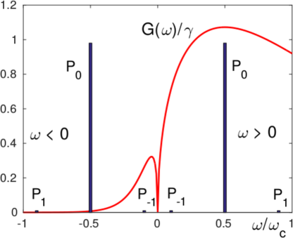
In the limit of weak-modulation ($0\leq\mu\ll 1$), only the sidebands $m=0$ and $m=\pm 1$ have significant weights $P_{m}$ in the harmonic (Floquet) expansion of the system response klimovsky13 : the $m$th sideband weight $P_{m}$, corresponding to the Floquet (harmonic) frequency $\omega_{m}=\omega_{0}+m\Delta$, falls off rapidly with increasing $|m|$. The QFI can then be written as (see App. D)

$$\mathcal{H} = \mathcal{H}_{-1}+\mathcal{H}_{0}+\mathcal{H}_{1};$$

$$\mathcal{H}_{\pm 1} = \frac{P_{\pm 1}e^{\frac{\omega_{\pm 1}}{T}}\omega_{\pm 1}^{2}}{\left(-1+e^{\frac{\omega_{\pm 1}}{T}}\right)^{2}T^{4}},$$ (7)

Here $\mathcal{H}_{\pm 1}$ are the contributions to the QFI arising from to the $m=\pm 1$ sidebands with $P_{\pm 1}\simeq\mu^{2}/4$, and $\mathcal{H}_{0}$ includes the $m=0$ contribution.

The advantages of DCQT are then revealed for a control scheme with $\Delta$ chosen such that

$$\omega_{-1}\sim T\ll\omega_{0},\omega_{1},$$ (8)

so that

$$\varrho_{n}=\frac{1}{N_{\rm avg}+1}\left(\frac{N_{\rm avg}}{N_{\rm avg}+1}\right)^{n}$$ (9)

with the average occupation number given by

$$N_{\rm avg} = N_{\rm eff}\approx\frac{1}{\frac{1}{P_{1}}e^{\omega_{-1}/T}-1}$$ (10)

The QFI is then predominantly associated with the $\mathcal{H}_{-1}$ term, with the maximum located at the temperature

$$T\approx T_{-1}:=\left(\omega_{0}-\Delta\right)/4=\omega_{-1}/4.$$ (11)

If higher sidebands ($|m|\geq 2$) are taken into account, the results remain valid, except for a marginal increase of the relative error bound $\xi$ at low temperatures (see Apps. LABEL:B-LABEL:E).

By contrast, in the absence of any control ($\mu=0$), $\varrho_{n}$ is still given by Eq. (8), with the average phonon occupation number

$$N_{\rm avg}=N_{0}=\frac{1}{e^{\omega_{0}/T}-1},$$ (12)

which vanishes in the limit $T\ll\omega_{0}$. The corresponding QFI is given by

$$\mathcal{H}(\mu=0)=\mathcal{H}_{0}(\mu=0)=\frac{e^{\frac{\omega_{0}}{T}}\omega_{0}^{2}}{\left(-1+e^{\frac{\omega_{0}}{T}}\right)^{2}T^{4}},$$ (13)

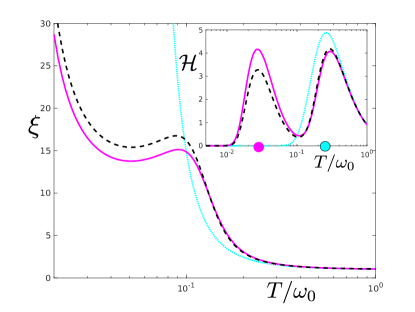
which has a single peak at $T=T_{0}$, where $T_{0}$ satisfies the equation $T_{0}=\omega_{0}\coth\left(\omega_{0}/2T_{0}\right)/4$ (Cf. inset of Fig. 2).

One can infer from the above results that a weak sinusoidal modulation (small $\mu$) with appropriately large $\Delta$ results in a double-peaked QFI, attaining maxima at $T\approx T_{-1}$ and $T\approx T_{0}$, owing to contributions from $\mathcal{H}_{-1}$ and $\mathcal{H}_{0}$ respectively (Fig. 2). This double peaked QFI signifies the applicability of DCQT for estimating a much broader range of temperatures, viz., in the vicinity of $T=T_{-1}$, which can be tuned according to our temperature of interest by tuning $\omega_{-1}$, and $T=T_{0}$. In comparison, an uncontrolled quantum thermometer can accurately measure temperatures only in the vicinity of $T=T_{0}$ for probes characterized by a single energy gap, or at multiple fixed (untunable) temperatures, for probes characterized by highly degenerate multiple energy-levels with arbitrary spacings campbell18precision .

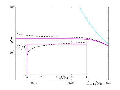
For a sub-Ohmic bath spectrum with a low-frequency edge $\omega_{\rm min}$, the minimum error bound $\xi(T=T_{-1})$ per measurement ($\mathcal{M}=1$) remains finite and approximately constant at (see App. D)

$$\lim_{\Delta\uparrow\omega_{0}}\xi(T=T_{-1}\gtrsim\omega_{\rm min}/4)\to\frac{\exp\left(2\right)}{2\mu},$$ (14)

where $\Delta\uparrow\omega_{0}$ signifies $\Delta$ approaching $\omega_{0}$ from below. Condition (14) yields the maximum possible advantage offered by our control scheme close to the absolute zero (i.e., for $T\approx T_{-1}\ll\omega_{0}$), and is valid in the regime

$$G_{0}\ll\omega_{-1}\sim T;\leavevmode\nobreak\ \leavevmode\nobreak\ \omega_{\rm min}<\omega_{-1}\sim T.$$ (15)

An error bound $\xi$ which does not diverge at low temperatures $T\ll\omega_{0}$ (as in standard quantum thermometry), but instead stays constant as the temperature decreases in that range, is deemed to be highly advantageous, since it allows us to measure such low temperatures. We have thus obtained a remarkable result: the advantage offered by our control scheme, expressed by the bound Eq. (14) close to the absolute zero (i.e., for $T\ll\omega_{0}$), is maximal for a sub-Ohmic, nearly-flat bath spectrum (NFBS) with small, but non-zero, lower edge, such that the bath interacts weakly with the DCQT at all non-zero frequencies. Regime (15) ensures that the dynamics is Markovian (see Methods).

Conditions (14), (15) allow us to achieve thermometry with a high-precision bound for very low temperatures; viz., only a finite number of measurements $\mathcal{M}\gg e^{4}/(4\mu^{2})$ ensures a relative error bound which is constant, i.e., temperature-independent, and has the finite value $\exp\left(2\right)/2\mu\sqrt{\mathcal{M}}$. For given small values of $G_{0}$ and $\omega_{\rm min}$, we then arrive at a minimum (limiting) temperature bound that is measurable with the error bound (14) per measurement:

$$T = {\rm max}\left[T_{\rm lim1},T_{\rm lim2}\right];$$

$$T_{\rm lim1} \gg G_{0};\leavevmode\nobreak\ \leavevmode\nobreak\ \leavevmode\nobreak\ T_{\rm lim2}>\omega_{\rm min},$$ (16)

In particular, for a sub-Ohmic NFBS (Eq. (5)) coupled very weakly with the thermometer at all frequencies such that $G_{0}\ll\omega_{\rm min}\to 0$, one has $T_{\rm lim}\to 0$, thus enabling us (at least under ideal circumstances, i.e., in absence of any other source of error) to accurately measure temperatures very close to the absolute zero.

The only penalty for a small $G_{0}\ll\omega_{\rm min}$ is long thermalization time. Yet, even if $G_{0}$ corresponds to divergent thermalization times (e.g., for $G_{0},\omega_{\rm min}\to 0$), one can use optimal control to reach the steady state at the minimal (quantum speed limit) time sugny10 : one can initially apply a strong brief pulse to take the thermometer to an optimal state, from which it takes the least time to thermalize, as detailed in mukherjee13 . Following this initial pulse, one can periodically modulate the system, as presented here. This behavior is in sharp contrast to that of an unmodulated thermometer, where $\xi(T)$ diverges for $T\to 0$, thus precluding any possibility of precise temperature estimation at very low temperatures potts19fundamental .

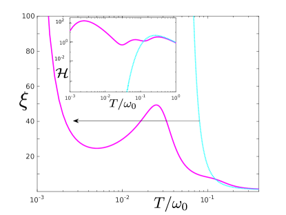
This novel effect of keeping $\xi$ finite even in close proximity to the absolute zero is a direct consequence of our control scheme, and is unachievable without modulation for any non-zero $\omega_{0}$. Extension of the analysis to multipeak QFI is given in the App. F (also see Fig. (4)).

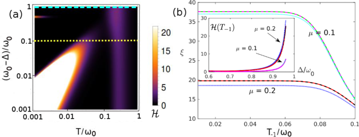
As discussed above, optimal thermometry demands choosing a $\Delta$ such that the QFI has a maximum at the temperature regime of interest, which is always possible for small enough $\omega_{\rm min}$ (cf. Eq. (16)). However, even for a bath spectrum with small but finite $\omega_{\rm min}$, one can perform low-temperature thermometry with a low relative error bound in the regime $G_{0}\ll T<\omega_{\rm min}$ via sub-optimal DCQT whose response is peaked at a temperature close to, but larger than $\omega_{\rm min}$. In this case the QFI, albeit not maximal, would be still significantly higher than that of the same thermometer in the absence of dynamical control. For example, in order to measure temperatures of the order $T\sim 10^{-3}\omega_{0}$, ideally one would need $\omega_{m}\sim 10^{-3}\omega_{0}$. However, even a suboptimal modulation with $\omega_{m}\sim 10^{-2}\omega_{0}$, which leads to QFI with a maximum at $T\sim\omega_{m}\sim 10^{-2}\omega_{0}$, results in $\mathcal{H}\approx 14.3$ at $T=10^{-3}\omega_{0}$ (see inset of Fig. (4)). In contrast, $\mathcal{H}$ is vanishingly small (i.e., $\mathcal{H}\ll 1/T^{2}$ such that $\xi\gg 1/\sqrt{\mathcal{M}}$; Cf. Eq. (3)) for the same temperature regime in the absence of control, thus exhibiting the advantage of our DCQT even for suboptimal thermometry at $T<\omega_{\rm min}$.

Figure 3: Temperature-independent relative error bound with dynamical control: Relative error bound $\xi$ for the estimation of bath temperature at $T=T_{-1}=(\omega_{0}-\Delta)/4$, by a harmonic oscillator dynamically controlled quantum thermometer under sinusoidal modulation (Cf. Eq. (6)), for the following bath spectra: nearly flat bath spectrum (magenta solid curve), sub-Ohmic bath spectrum with $s=0.1,\omega_{c}=100$ (black dashed curve) and the same spectra in the absence of control (turquoise dotted curve). Dynamical control reduces the relative error bound significantly, with $\xi$ remaining constant over a broad range of low temperatures $T\ll\omega_{0}$. The sidebands $m=0,\pm 1,\pm 2,\pm 3$ are included in the calculation. Here the modulation amplitude $\mu=0.2$, and $\omega_{0}=1$. Inset: Corresponding spectral response functions scaled by $\gamma$.

Figure 4: Dynamical control with multiple harmonics: Relative error bound $\xi$ and Quantum Fisher Information $\mathcal{H}$ (in inset) as a function of temperature $T$ (in units of $\omega_{0}$) in the absence of any modulation (turquoise dotted curve) and under multi-harmonic modulation $\omega(t)=\omega_{0}+\Delta\left(\mu_{l}\sin\left(lt\Delta\right)+\mu_{l^{\prime}\neq l}\sin\left(l^{\prime}t\Delta\right)\right)$ (magenta solid curve), for harmonic oscillator dynamically controlled quantum thermometer probing a bath with nearly-flat bath spectrum. Our control scheme reduces the lowest temperatures measurable with finite $\xi$ by almost two orders of magnitude (arrow). Here $l=80,\leavevmode\nobreak\ l^{\prime}=99,\leavevmode\nobreak\ \mu_{80}=0.394,\leavevmode\nobreak\ \mu_{99}=0.115,\leavevmode\nobreak\ \leavevmode\nobreak\ \Delta=0.01$, $\omega_{0}=1$, $\omega_{\rm min}\ll 0.01$ and $\mathcal{M}=1$.

Thermometry of arbitrary bath spectra: The advantage offered by DCQT is not restricted to the specific bath spectra considered above. In fact, the key result of significant improvement in low-temperature thermometry by dynamical control holds for arbitrary bath spectra satisfying the Kubo-Martin-Schwinger condition (see Eq. (30) of Methods), as long as $G(\omega>0)$ is independent of temperature. Choosing a control scheme satisfying (see Eq. (11))

$$\omega_{-1}=\kappa T$$ (17)

for a positive constant $\kappa$ of the order of unity, leads to a QFI which diverges quadratically with temperature:

$$\mathcal{H}\approx\frac{\eta e^{\kappa}\kappa^{2}}{\left(-1+\eta e^{\kappa}\right)^{2}T^{2}}.$$ (18)

The above result Eq. (18), which is valid for any bath spectra, arises due to $\omega_{-1}$ being vanishingly small (see Eq. (17)). The lowest temperature for which Eq. (18) is valid is given by the condition

$$\omega_{-1}\sim T\gg T_{\rm lim}=G(\omega_{-1}).$$ (19)

As in the case of sub-Ohmic NFBS, condition (19) ensures that the thermalization time is long enough for the secular approximation to remain valid. This in turn results in a relative error bound

$$\xi \approx \sqrt{\frac{\left(-1+\eta e^{\kappa}\right)^{2}}{\eta\kappa^{2}e^{\kappa}}}\frac{1}{\sqrt{\mathcal{M}}},$$

$$\eta = \frac{P_{0}G(\omega_{0})+P_{1}\left(G(\omega_{1})+G(\omega_{-1})\right)}{P_{1}G(\omega_{-1})}.$$ (20)

which is not explicitly dependent on the temperature, even for low temperatures $T\ll\omega_{0}$ (see Fig. (3)). Although the relative error bound $\xi$ is not explicitly dependent on temperature, the QFI and consequently $\xi$ still depend on the details of the bath spectral function $G(\omega)$ at $\omega=\omega_{-1}$, which in turn is determined by the temperature through Eq. (17). The maximum QFI in this case is obtained by modulations satisfying the optimal condition

$$P_{1}G(\omega_{-1})\gg P_{0}G(\omega_{0}),P_{1}G(\omega_{1}).$$ (21)

The above condition ensures that the sidebands $m\neq-1$ are insignificant, so as to yield a small relative error bound at $T\sim\omega_{-1}$ (see App. C).

Condition (21) shows that one needs to tailor the control scheme to the bath spectrum at hand. For example, in the case of a bath spectrum characterized by $G(\omega_{0})\gg G(\omega_{-1})$, one needs to design a modulation with $P_{-1}\gg P_{0}$, in order for our control scheme to be beneficial for estimating temperatures $T\sim T_{-1}\ll\omega_{0}$. This can be realized using a periodic $\pi$-pulse modulation, in which case $P_{\pm 1}\approx 4/\pi^{2}$ and $P_{m\neq\pm 1}\approx 0$ klimovsky13 .

Discussion

We have shown that by subjecting a generic quantum thermometer to an appropriate dynamical control, we may increase its maximum accuracy bound of measuring a chosen range of temperatures. The class of quantum thermometers considered here relies on the measurement of the energy-level populations $\varrho_{n}$ at the steady-state, as well as knowledge of the resonant frequency $\omega_{0}$ of the thermometer, the modulation parameters $\mu$ and $\Delta$ (cf. (6)) and (at least crudely) the bath spectral density $G(\omega)$ (see App. A). It falls in the category of secondary thermometers. The advantage of the proposed DCQT becomes especially apparent at low temperatures, where, for generic bath spectra $G(\omega)$, its accuracy bound of measuring the bath temperature, quantified by the QFI, is dramatically higher than that of its unmodulated counterpart. Namely, dynamical control allows us to perform low-temperature thermometry with temperature-independent relative error bound, at temperatures above the bound set by Eq. (16). Our proposed control scheme can be tailored according to the bath spectra at hand, in order to maximize the QFI, and determine the number of its peaks and sensitivity ranges, thus making it highly versatile.

In addition to our diagonal Hamiltonian $\hat{H}(t)=\sum_{n=0}^{\mathcal{N}}\omega_{n}(t)|n\rangle\langle n|$, off-diagonal interaction terms of the form $\sum_{n,m=0}^{\mathcal{N}}\left(h_{n,m}|n\rangle\langle m|+h.c.\right)$ may incur non-adiabatic effects, which may cause spurious transitions between the energy levels, even in the absence of any external bath. In order to avoid such excitations one should require $\omega(t)\gg h_{n,m}$ for all $t,n,m$, thereby ensuring adiabaticity.

The dynamical control studied here has already been realized experimentally, in the context of probing the system-environment coupling spectrum almog11direct . One can utilize similar dynamical control to realize DCQT in different multilevel systems (see App. A): i) a harmonic oscillator DCQT can be implemented by the mode of a cavity of length $l(t)$, whose frequency $\omega(t)\propto 1/l(t)$ is modulated with the inverse of the cavity length macri18nonperturbative . ii) A two-level DCQT can be implemented by a qubit whose level spacing is modulated by a time-dependent magnetic field, for example in NMR prigl96a and NV-center casola18probing experiments. Experimentally, one can probe the thermal steady-state $\hat{\rho}(t\to\infty)$ of the DCQT at large times, after decoupling it from the bath, followed by ceasing the dynamical control (i.e., first setting $\gamma=0$, and then $\mu=0$). In a harmonic-oscillator thermometer one can then estimate the temperature $T$ through measurement of the mean number of quanta of the thermometer $N_{\rm avg}$, for example through motional sideband spectroscopy, which relies on the asymmetry between phonon absorption (proportional to $N_{\rm avg}$) and phonon emission (proportional to $N_{\rm avg}+1$) safavi-naeini12observation . In a two-level NV-center thermometer hopper18spin ; tran18anti , spin readout using photoluminescence may enable us to measure the N-V temperature.

The thermal energy-level population measurements $\varrho_{n}$ (see Eq. (9)), which constitute the optimal positive-operator valued measure for estimating temperature brunelli11 , are characterized solely by the average number of quanta $N_{\rm avg}$. Consequently, measurement of $N_{\rm avg}$ gives us the complete knowledge of $\hat{\rho}(t\to\infty)$, which in turn enables us to approach the minimum error bound $\xi$ of bath-temperature estimation. However, while DCQT can dramatically reduce the error bound of temperature estimation (see Eqs. (19) and (60)), additional experimental errors may arise from the finite accuracy of measuring $\Delta$, or the energy-level populations. These errors, which depend on the experimental apparatus, may prevent us from reaching the fundamental theoretical bound of Eq. (60) (see App. B).

DCQT can be highly advantageous for thermometry of diverse baths realized by many-body quantum systems in condensed matter and ultracold atomic gases, with spectra and modulations satisfying the optimal condition Eq. (21).

The temperatures measurable with low relative error bound using our control scheme are presented in Table 1.

Parameters	Values
$\omega_{-1}$	$\sim 10^{x}$ Hz
$T_{-1}$	$\approx 1.9\times 10^{x-12}$ K
$\small{\mathcal{H}(T=T_{-1})}$	$\approx\frac{P_{1}e^{\frac{\hbar\omega_{-1}}{k_{B}T}}\hbar^{2}\omega_{-1}^{2}}{\left(-P_{1}+e^{\frac{\hbar\omega_{-1}}{k_{B}T}}\right)^{2}k_{B}^{2}T^{2}}\frac{1}{T^{2}}{\rm K}^{-2}\approx\frac{4\mu^{2}}{e^{4}}\frac{1}{T^{2}}{\rm K}^{-2}$
$\xi(T=T_{-1})$	$\approx\exp\left(2\right)/\left(2\mu\sqrt{\mathcal{M}}\right)$

Table 1: Illustrative values: Values of $T_{-1}=\hbar\omega_{-1}/4k_{B}$, quantum Fisher information $\mathcal{H}(T=T_{-1})$ and relative error bound $\xi(T=T_{-1})$ for $\omega_{-1}=\omega_{0}-\Delta\sim 10^{x}$ Hz, for a harmonic oscillator dynamically controlled quantum thermometer under sinusoidal modulation probing a nearly-flat bath spectrum. Here $x$ is a real number.

In a microwave cavity subjected to sinusoidal modulation with $\omega_{0}-\Delta\sim 10^{x}$ Hz, DCQT results in QFI attaining a peak at temperatures of the order of $10^{x-12}$ K, $x$ being real. We thereby open new avenues for the study of cavity quantum electrodynamics and quantum information processing hauke16 at extremely low temperatures. The caveat noted above is that although the dynamical control can be expected to significantly reduce the error in low-temperature thermometry, however, experimental errors may preclude the attainment of theoretical bound of temperature resolution.

DCQT can be expected to be highly beneficial in baths exhibiting the widely studied $1/f^{\alpha}$ ($\alpha\geq 0$) noise spectra milotti02onebyf in vacuum tubes johnson25the or in thick film resistors pellegrini83noise . This kind of spectra ensures that for a sinusoidal modulation with small $\omega_{-1}$, the most dominant contribution arises from the $m=-1$ sideband, thus enabling us to probe low frequencies with high precision bound.

An intriguing application of the proposed DCQT concerns experimentally studying the third law of thermodynamics for low-temperature many-body quantum systems, in the sense of understanding the scaling of the cooling rate with temperature masanes17a ; freitas17fundamental ; cleuren12 . In view of predictions that the cooling rate does not vanish as the absolute zero is approached for baths with anomalous dispersion, such as magnon (ferromagnetic) spin chains kolar12 , high-precision low-temperature thermometry is imperative.

In many-body quantum systems rigol08 ; eisert15 ; calabrese11 ; alvarez15 ; kaufman16 , interactions may keep a system non-equilibrated for a long time after a quench breuer02 , during which time its different collective modes $k$ may have their own temperatures $T_{k}$. High-precision multi-mode thermometry over a wide range of temperatures using our DCQT can verify whether different modes have different temperatures, and thus avoid thermalization.

The versatility of our DCQT can be well-suited for simultaneous multi-mode probing of a bath with high accuracy bound, which can be especially useful for nanometer-scale thermometry in biological systems kucsko13 ; baffou14a .

The recently discussed need for thermometers with vanishing energy gaps for measuring low-temperatures in many-body quantum systems potts19fundamental and in strongly coupled quantum systems hovhannisyan18measuring , suggests the importance of control schemes capable of tuning the gap of a quantum thermometer to our advantage. Application of our control scheme to thermometers modelled by many-body quantum systems, or to thermometers coupled strongly to the bath, in order to achieve high-precision low-temperature thermometry, is an interesting question which we aim to address in the future.

The control scheme presented above may have diverse applications in quantum metrology beyond thermometry. For example, periodic modulation of energy levels in many-body quantum critical systems may be applicable to precise probing of inter-particle coupling strengths in these systems zanardi08quantum .

Methods

Thermalization under periodic modulation

We consider a multi-mode DCQT system with its state $\rho(t)$ given as a direct product of single-mode states $\rho_{k}$: $\rho(t)=\otimes_{k}\rho_{k}(t)$, interacting with a multi-mode bath, again described by the direct product state $\rho_{B}=\otimes_{k}\rho_{B_{k}}$. Here $\rho_{B_{k}}$ denotes the state of the $k$-th mode of the bath. For each $k$, $\rho_{k}(t)$ evolves under the action of a periodic Hamiltonian, satisfying Eq. (1). The system is coupled to the bath mode through the interaction Hamiltonian

$$\hat{H}_{Ik}=\hat{S}_{k}\otimes\hat{B}_{k},$$ (22)

where each of the independent $k$-th mode baths has a spectrum wide enough to give rise to Markovian dynamics; for example, a finite-Q cavity mode, or a finite-lifetime phonon mode. In case the above assumption is violated, leading to non-Markovian dynamics breuer02 ; zwick14 , the DCQT may be useful for revealing the absence of thermalization. Here we allow for baths with mode-dependent temperatures $T_{k}$, which we aim to measure accurately using our DCQT.

We sketch below the derivation of the master equation describing the thermalization of a system under periodic control. We refer to breuer02 ; klimovsky13 ; klimovsky15 ; alicki14 for details of the derivation, and almog11direct for experimental studies of open quantum system in presence of dynamical control. (For reviews on periodically driven open quantum systems, see klimovsky15 ; kosloff13 .)

The time evolution operator for the periodic Hamiltonian Eq. (1) is given by

$$\hat{U}_{k}(t,0)=\hat{\mathcal{T}}\exp\left(-i\int^{t}_{0}\hat{H}_{k}(t^{\prime})dt^{\prime}\right),$$ (23)

$\hat{\mathcal{T}}$ being the time ordering operator. According to the Floquet theorem, one can decompose the time evolution operator as $\hat{U}_{k}(t,0)=\hat{P}_{k}(t)e^{\hat{R}_{k}t}$, where $\hat{P}_{k}(t+\tau)=\hat{P}_{k}(t)$ and $\hat{R}_{k}$ is a constant operator. Taking into account $\hat{U}_{k}(0,0)=\mathds{1}$, and the periodicity of $\hat{P}_{k}(t)$, one obtains $\hat{P}_{k}(0)=\mathds{1}$ and hence $\hat{U}_{k}(\tau,0)=\hat{P}_{k}(\tau)e^{\hat{R}_{k}\tau}=\hat{P}(0)e^{\hat{R}_{k}\tau}=e^{\hat{R}_{k}\tau}$. One can now identify the operator $\hat{R}_{k}$ with an effective Hamiltonian $\hat{H}_{k,\rm eff}$ averaged over a period of $\hat{H}_{k}(t)$, as

$$\hat{U}_{k}(\tau,0)=e^{\hat{R}_{k}\tau}=:e^{-i\hat{H}_{k,\rm eff}\tau},$$ (24)

with eigenenergies $\Omega_{k,r}$ and eigenstates $|r_{k}\rangle$, through the relation

$$\hat{H}_{k,\rm eff}=\sum_{r}\Omega_{k,r_{k}}|r_{k}\rangle\langle r_{k}|.$$ (25)

The Fourier components $\hat{S}_{\omega_{k},m}$ of the system operator $\hat{S}_{k}(t)$ (Cf. Eq. (22)) in the interaction picture with respect to the evolution (23), are given as

$$\hat{S}_{k}(t) = \hat{U}_{k}^{\dagger}(t,0)\hat{S}_{k}\hat{U}_{k}(t,0)$$ (26)

$$= \sum_{\{\omega_{k}\}}\sum_{m\in\mathbb{Z}}\hat{S}_{\omega_{k},m}e^{i\left(\omega_{k}+m\Delta\right)t},$$

where $\Delta=2\pi/\tau$, $m$ are integers, and $\{\omega_{k}\}$ is defined as the set of all transition frequencies $\Omega_{k,r^{\prime}}-\Omega_{k,r}$ between the levels of $\hat{H}_{k,\rm eff}$ and the operators $\hat{S}_{\omega_{k},m}$ are the $m$th-harmonic transition operators associated with these levels klimovsky15 .

Next we focus only on the dynamics of the $k$-th mode of the thermometer and the bath. Under the standard Born-Markov approximation in the weak thermometer-bath coupling limit, we arrive at the master equation breuer02

$$\frac{d}{dt}\hat{\rho}_{k}(t)$$

$$= -\int^{\infty}_{0}ds{\rm Tr}_{B_{k}}\Big{[}H_{Ik}(t),\left[\hat{H}_{Ik}(t-s),\hat{\rho}_{k}(t)\otimes\hat{\rho}_{B_{k}}\right]\Big{]},$$

where ${\rm Tr}_{B_{k}}$ denotes trace over the bath mode $k$, and $\hat{H}_{Ik}(t)$ is the $k$-th mode interaction Hamiltonian in the interaction picture.

We now assume that the thermalization time of the thermometer induced by the bath is much longer than $\tau$ or $\omega_{k,m}^{-1}\equiv\left(\omega_{k}+m\Delta\right)^{-1}$. Consistently, we adopt the secular approximation (SA) to average out the rapidly oscillating terms of the form $\exp\left[\pm i\left(\omega_{k,m}-\omega_{k^{\prime},m^{\prime}}\right)t\right]$ at times $t\gg\tau,\omega_{k,m}^{-1}$, such that only the terms with $k=k^{\prime},\leavevmode\nobreak\ m=m^{\prime}$ survive mukherjee16speed . We then finally arrive at the master equation klimovsky13 ; klimovsky15 ; alicki14 ; breuer02 , which is a weighted sum of Lindbladian superoperators, each valid for system-bath coupling centered at $\omega_{k,m}:=\omega_{k}+m\Delta$:

$$\dot{\hat{\rho}}_{k}(t)=\mathcal{L}_{k}\left[\hat{\rho}_{k}(t)\right]=\sum_{\{\omega_{k}\}}\sum_{m}\mathcal{L}_{\omega_{k},m}\left[\hat{\rho}_{k}(t)\right].$$ (28)

Here

$$\mathcal{L}_{\omega_{k},m}\left[\hat{\rho}_{k}(t)\right] = G(\omega_{k}+m\Delta)\mathcal{D}_{\omega_{k},m}[\hat{\rho}_{k}(t)]$$

$$+ G(-\omega_{k}-m\Delta)\mathcal{D}_{\omega_{k},m}^{\dagger}[\hat{\rho}_{k}(t)],$$

$$\mathcal{D}_{\omega_{k},m}[\hat{\rho}_{k}(t)] = \Big{(}\hat{S}_{\omega_{k},m}\hat{\rho}_{k}(t)\hat{S}^{\dagger}_{\omega_{k},m}$$ (29)

$$- \frac{1}{2}\hat{S}^{\dagger}_{\omega_{k},m}\hat{S}_{\omega_{k},m}\hat{\rho}_{k}(t)$$

$$- \frac{1}{2}\hat{\rho}_{k}(t)\hat{S}^{\dagger}_{\omega_{k},m}\hat{S}_{\omega_{k},m}\Big{)},$$

and

$$G(\pm\left(\omega_{k}+m\Delta\right))$$

$$= \int_{-\infty}^{\infty}e^{\pm i\left(\omega_{k}+m\Delta\right)t}\langle\hat{B}_{k}(t)\hat{B}_{k}(0)\rangle dt,$$

where $\hat{B}_{k}(t)=e^{i\hat{H}_{B}t}\hat{B}_{k}e^{-i\hat{H}_{B}t}$, $\hat{H}_{B}$ being the bath Hamiltonian, represents the bath spectral response or auto-correlation function sampled at the frequency harmonics $\pm\left(\omega_{k}+m\Delta\right)$. The Kubo-Martin-Schwinger condition must be imposed, i.e.,

$$\frac{G(\omega_{k}+m\Delta)}{G(-\omega_{k}-m\Delta)}=\exp\left[\left(\omega_{k}+m\Delta\right)/T_{k}\right].$$ (30)

Eqs. (29) - (30) imply that, within the approximations assumed above, $\rho_{k}$ equilibrates to a thermal (Gibbs) state at temperature $T_{k}$. The level populations are determined by the weighted bath response at the resonance frequencies $\omega_{k}$ shifted by Floquet harmonics of modulation, $\omega_{k,m}=\omega_{k}+m\Delta$.

Data availability

All relevant data are available to any reader upon reasonable request.

Code availability

All relevant codes are available to any reader upon reasonable request.

Author Contributions

V.M. and G.K. conceived the idea. V.M. and A.Z. performed the analytical calculations and numerical simulations. V.M., A.Z., A.G., X.C. and G.K. were involved in the interpretation of the results and in the discussions during the writing of the manuscript. V.M. and G.K. wrote the manuscript.

Appendix A $\mathcal{N}$ level dynamically controlled thermometer

A single bath probed by a single-mode $\mathcal{N}$ level system, subject to a (generic) diagonal modulation is described by the Hamiltonian

$$\hat{H}(t)=\sum_{n=0}^{\mathcal{N}}\omega_{n}(t)|n\rangle\langle n|=\sum_{n=0}^{\mathcal{N}}n\omega(t)|n\rangle\langle n|,$$ (31)

with

$$\omega_{0}=\frac{1}{\tau}\int^{\tau}_{0}\omega(t)dt,\leavevmode\nobreak\ \leavevmode\nobreak\ \leavevmode\nobreak\ \leavevmode\nobreak\ \hat{H}_{\rm eff}=\sum_{n=0}^{\mathcal{N}}n\omega_{0}|n\rangle\langle n|.$$ (32)

The interaction Hamiltonian has the form

$$\hat{H}_{I}=\hat{S}\otimes\hat{B},$$ (33)

where $\hat{S}$ is a system-operator belonging to a Lie algebra, and the operator $\hat{B}$ acts on the bath. Under modulation with period $\tau$ the master equation for the state of the system reduces to the Floquet expansion alicki12periodically ; szczygielski13 ; kosloff13 ; klimovsky13 ; klimovsky115laser ; klimovsky15 ; alicki14 ; breuer02 ; carmichael02 ; agarwal13 ; alicki18introduction ; kofman01universal ; kofman04unified ; gordon07universal ; clausen10bath ; shahmoon13 ; zwick14 ; mukherjee16speed ; sillanpaa09autler

$$\dot{\hat{\rho}}(t) = \sum_{m}\mathcal{L}_{m}\left[\hat{\rho}(t)\right]$$

$$\mathcal{L}_{m}[\hat{\rho}(t)] = \left[G(\omega_{m})\mathcal{D}_{m}[\hat{\rho}(t)]+G(-\omega_{m})\mathcal{D}_{m}^{\dagger}[\hat{\rho}(t)]\right]$$

$$\mathcal{D}_{m}[\hat{\rho}] = P_{m}\mathcal{D}[\hat{\rho}]$$

$$= \Big{(}\hat{S}_{m}\hat{\rho}\hat{S}_{m}^{\dagger}-\frac{1}{2}\hat{S}_{m}^{\dagger}\hat{S}_{m}\hat{\rho}-\frac{1}{2}\hat{\rho}\hat{S}_{m}^{\dagger}\hat{S}_{m}\Big{)}$$

$$\hat{S}_{m} = P_{m}\hat{S}_{-};\leavevmode\nobreak\ \leavevmode\nobreak\ \hat{S}_{m}^{\dagger}=P_{m}\hat{S}_{+}.$$ (34)

Figure 5: Floquet sidebands: A sub-Ohmic bath spectral function $G(\omega>0)=\gamma\left(\omega^{s}/\omega_{c}^{s-1}\right)\exp\left[-\omega/\omega_{c}\right]$ (scaled by $\gamma$) (red curve); $\gamma$ determines the amplitude of $G(\omega)$. According to the Kubo-Martin-Schwinger condition, $G(-\omega)=G(\omega)\exp\left(-\omega/T\right)$. The weights $P_{m}$ at frequencies $\omega_{m}=\omega_{0}+m\Delta$ are shown for a weak sinusoidal modulation (Eq. (45)) for $m=0,\pm 1$ (blue lines). As seen above, $P_{\pm 1}\ll P_{0}$. The higher sidebands ($|m|>1$) are associated with negligible weights $P_{m}$’s, and can be neglected in this regime. Here $s=0.5,\leavevmode\nobreak\ \omega_{c}=1,\leavevmode\nobreak\ \omega_{0}=0.5\omega_{c},\leavevmode\nobreak\ T=0.1\omega_{c},\leavevmode\nobreak\ \Delta=0.4\omega_{c}$ and $\mu=0.2$.

Here the Floquet sideband frequencies labeled by integer $m$ are $\omega_{m}=\omega_{0}+m\Delta$, $\Delta=2\pi/\tau$, $P_{m}=P_{-m}$ denotes the weight of the $m$-th sideband and $\hat{S}_{\pm}$ are the corresponding system excitation and deexcitation (ladder) operators. A physical bath has spectral response $G(\omega)$ that is non-zero and finite for $\omega>0$, satisfies $G(\omega\to 0)\to 0$. Here we consider $G(\omega>0)$ to be independent of temperature, while the Kubo-Martin-Schwinger (KMS) condition (Cf. Eq. (25) of main text), determines $G(\omega<0)$ through the relationbreuer02 :

$$G(-\omega)=G(\omega)e^{-\omega/T}.$$ (35)

For such bath-response spectra one can rewrite Eq. (34) as

$$\dot{\hat{\rho}}(t) = \sum\nolimits_{m}P_{m}\Big{[}G(\omega_{m})\mathcal{D}[\hat{\rho}(t)]+G(-\omega_{m})\mathcal{D}^{\dagger}[\hat{\rho}(t)]\Big{]}$$ (36)

$$= \Big{(}\sum\nolimits_{m}^{+}P_{m}G(\omega_{m})$$

$$+ \sum\nolimits_{m}^{-}P_{m}G(|\omega_{m}|)e^{-|\omega_{m}|/T}\Big{)}\mathcal{D}[\hat{\rho}(t)]$$

$$+ \Big{(}\sum\nolimits_{m}^{+}P_{m}G(\omega_{m})e^{-\omega_{m}/T}$$

$$+ \sum\nolimits_{m}^{-}P_{m}G(|\omega_{m}|)\Big{)}\mathcal{D}^{\dagger}[\hat{\rho}(t)].$$

Here $\sum_{m}$ denotes the Floquet summation over all integers $m$, while $\sum^{+}_{m}$ ($\sum^{-}_{m})$ denotes summation over integer $m$ such that $\omega_{m}\geq 0$ ($\omega_{m}<0$).

As the thermometer thermalizes with the bath, its state converges to the thermal (Gibbs) state upon neglecting the fast oscillating terms:

$$\hat{\rho}(t\to\infty) = \sum_{n=0}^{\mathcal{N}}\varrho_{n}|n\rangle\langle n|;$$

$$\varrho_{n} = \frac{e^{-n\omega_{\rm eff}/T}}{\sum_{n=0}^{\mathcal{N}}e^{-n\omega_{\rm eff}/T}},$$ (37)

where the probability ratios (Boltzmann factors) of levels $n$ and $n+1$ satisfy

$$\frac{\varrho_{n+1}}{\varrho_{n}} = e^{-\omega_{\rm eff}/T}$$ (38)

$$= \frac{\sum_{m}G(-\omega_{m})P_{m}}{\sum_{m}G(\omega_{m})P_{m}};\leavevmode\nobreak\ \leavevmode\nobreak\ m=0,\pm 1,\pm 2,\ldots$$

Taking into account the definition of $G(\omega)$ and the KMS condition, we get the general Floquet form of the Boltzmann factors

$$e^{-\omega_{\rm eff}/T}=\frac{\sum^{+}_{m}G(\omega_{m})P_{m}e^{-\omega_{m}/T}+\sum^{-}_{m}G(|\omega_{m}|)P_{m}}{\sum^{+}_{m}G(\omega_{m})P_{m}+\sum^{-}_{m}G(|\omega_{m}|)P_{m}e^{-|\omega_{m}|/T}}.$$ (39)

From Eq. (39) for the asymptotic thermalized populations, we may calculate the quantum Fisher Information (QFI), which is defined as correa15 ; paris09

$$\mathcal{H} = -2\lim_{\epsilon\to 0}\partial^{2}F(\hat{\rho}(T,t),\hat{\rho}(T+\epsilon,t))/\partial\epsilon^{2}$$ (40)

$$= \sum_{n=0}^{\mathcal{N}}\frac{|\frac{\partial\varrho_{n}}{\partial T}|^{2}}{\varrho_{n}},$$

where $F(\hat{\rho}_{1},\hat{\rho}_{2})={\rm Tr}\left[\sqrt{\sqrt{\hat{\rho}_{1}}\hat{\rho}_{2}\sqrt{\hat{\rho}_{1}}}\right]$ is the fidelity between $\hat{\rho}_{1}$ and $\hat{\rho}_{2}$. This expression can be shown to assume the generic form

$$\mathcal{H}=\sum_{m}f(\{G_{m}\},\{P_{m}\},\{\exp\left(-|\omega_{m}|/T\right)\},\frac{\{\omega_{m}\}}{T^{2}},\mathcal{N}).$$ (41)

Here $\{x_{m}\}$ denotes the set of all $x_{m}$, and $f$ is an analytic functional form.

In the regime of weak modulation (see App. B below) and $\Delta<\omega_{0}$, all the leading harmonics contributing significantly to the dynamics are associated with $\omega_{m}>0$, and one can neglect all terms with $\omega_{m}<0$. In Fig. (5) we show as an example a sub-Ohmic bath spectrum satisfying the KMS condition, and the $P_{m}$’s due to a weak sinusoidal modulation (see Eq. (45) below). Eq. (39) then reduces to

$$\frac{\varrho_{n+1}}{\varrho_{n}}=e^{-\omega_{\rm eff}/T}\approx\frac{\sum^{+}_{m}G(\omega_{m})P_{m}e^{-\omega_{m}/T}}{\sum^{+}_{m}G(\omega_{m})P_{m}}.$$ (42)

It is seen that the $m$-th sideband contributes significantly to the Boltzmann factors in the steady state for $\omega_{m}\lesssim T$, provided $P_{m}G(\omega_{m})$, also known as the spectral-filter values kofman01universal ; kofman04unified , is large enough. The explicit form of the QFI is obtained from Eqs. (40) and (42) as

$$\mathcal{H}\approx\frac{A_{\rm gen}}{B_{\rm gen}},$$ (43)

where,

$$A_{\rm gen}=\sum_{n=0}^{\mathcal{N}}\left(\left(\frac{\kappa}{\zeta}\right)^{-2+n}\left(-\kappa\sum_{n=0}^{\mathcal{N}}\frac{n\left(\frac{\kappa}{\zeta}\right)^{-1+n}C}{\zeta}+n\left(\sum_{n=0}^{\mathcal{N}}\left(\frac{\kappa}{\zeta}\right)^{n}\right)C\right)^{2}\right),$$

$$B_{\rm gen}=T^{4}\zeta^{2}\Big{(}\sum_{n=0}^{N}\Big{(}\frac{\kappa}{\zeta}\Big{)}^{n}\Big{)}^{3},$$

and

$$C=\sum_{m}e^{-\frac{\omega_{m}}{T}}P_{m}G_{m}\omega_{m};\quad\kappa=\sum_{m}e^{-\frac{\omega_{m}}{T}}P_{m}G_{m};$$

$$\zeta=\sum_{m}P_{m}G_{m};\quad\quad\quad\omega_{m}>0.$$ (44)

As shown for specific examples in the main text, as well as in Apps. B - D, the QFI in Eq. (41) can be strongly enhanced at specific $T$ by an appropriate choice of the leading Floquet harmonics (sidebands) for a given bath response spectrum (see Fig. 6a for the QFI dependence on modulation frequencies and bath temperatures, considering the zeroth and the first three sidebands). Because of the restriction $\sum_{m}P_{m}=1$, in general only a few of the harmonics, which correspond to the frequency of the unmodulated system shifted by low multiples of the modulation frequency $\Delta$, contribute to the expressions for $A_{\rm gen}$, $B_{\rm gen}$, and thus to the QFI.

Appendix B Generic bath spectrum

Here we focus on a harmonic oscillator dynamically controlled quantum thermometer (DCQT) under a weak (small-amplitude) sinusoidal modulation

$$\hat{H}(t) = \omega(t)\hat{a}^{\dagger}\hat{a}=\sum_{n=0}^{\infty}n\omega(t)|n\rangle\langle n|,$$

$$\omega(t) = \omega_{0}+\mu\Delta\sin\left(t\Delta\right),$$ (45)

with $0<\mu\ll 1$.

For $\hat{S}=\left(\hat{a}+\hat{a}^{\dagger}\right)$, the interaction Hamiltonian becomes

$$\hat{H}_{I}=\left(\hat{a}+\hat{a}^{\dagger}\right)\otimes\hat{B}.$$ (46)

In the interaction picture, we have

$$\hat{S}(t) = \hat{U}^{\dagger}(t,0)\hat{S}\hat{U}(t,0)$$ (47)

$$= \exp\left[{-i\int^{t}_{0}\omega(t^{\prime})\hat{a}^{\dagger}\hat{a}dt^{\prime}}\right]\hat{S}$$

$$\exp\left[{i\int^{t}_{0}\omega(t^{\prime})\hat{a}^{\dagger}\hat{a}dt^{\prime}}\right],$$

which one can expand as

$$\hat{S}(t) = \sum_{m}\left[\varepsilon_{m}e^{-i\left(\omega_{0}+m\Delta\right)t}\hat{a}+\varepsilon_{m}^{*}e^{i\left(\omega_{0}+m\Delta\right)t}\hat{a}^{\dagger}\right],$$

$$m = 0,\pm 1,\pm 2,\pm 3,\ldots.$$ (48)

From Eqs. (47) and (48), one can show that the harmonic weights are given by alicki12periodically ; klimovsky13 ; klimovsky15

$$P_{m} = |\varepsilon_{m}|^{2}=\left|\frac{1}{\tau}\int^{\tau}_{0}e^{-i\int_{0}^{t}\left(\omega(t^{\prime})-\omega_{0}\right)dt^{\prime}}e^{it\Delta}dt\right|^{2}$$ (49)

$$= P_{-m}.$$

The weights $P_{m}$ can be evaluated in terms of Bessel functions. Since we assume that the amplitude $\mu\ll 1$, the lowest order terms are given by klimovsky13 ; alicki14 ; klimovsky15

$$P_{0} \approx 1-\frac{\mu^{2}}{2}+\frac{3\mu^{4}}{32}-\frac{5\mu^{6}}{576}+\mathcal{O}\left(\mu^{8}\right),$$

$$P_{\pm 1} \approx \frac{\mu^{2}}{4}-\frac{\mu^{4}}{16}+\frac{5\mu^{6}}{768}+\mathcal{O}\left(\mu^{8}\right),$$

$$P_{\pm 2} \approx \frac{\mu^{4}}{64}-\frac{\mu^{6}}{384}+\mathcal{O}\left(\mu^{8}\right),$$

$$P_{\pm 3} \approx \frac{\mu^{6}}{2304}+\mathcal{O}\left(\mu^{8}\right).$$ (50)

These weights decrease rapidly with increasing harmonic index $m$.

Unless otherwise stated, we consider below the limit $\Delta\uparrow\omega_{0}$, where we define $A\uparrow B$ as $A$ approaching $B$ from below. In this case $\omega_{m}<0$ for $m\leq-2$, while $\omega_{m}>0$ for $m\geq-1$. The master equation (36) is then evaluated to be

$$\dot{\hat{\rho}}(t) \approx C_{1}\left(\hat{a}\hat{\rho}(t)\hat{a}^{\dagger}-\frac{1}{2}\hat{a}^{\dagger}\hat{a}\hat{\rho}(t)-\frac{1}{2}\hat{\rho}(t)\hat{a}^{\dagger}\hat{a}\right)$$ (51)

$$+ C_{2}\left(\hat{a}^{\dagger}\hat{\rho}(t)\hat{a}-\frac{1}{2}\hat{a}\hat{a}^{\dagger}\rho(t)-\frac{1}{2}\hat{\rho}(t)\hat{a}\hat{a}^{\dagger}\right),$$

where

$$C_{1}=\Big{[}G(\omega_{0})P_{0}+P_{1}\left(G(\omega_{1})+G(\omega_{-1})\right)+P_{2}\left(G(\omega_{2})+G(|\omega_{-2}|)e^{-|\omega_{-2}|/T}\right)+P_{3}\left(G(\omega_{3})+G(|\omega_{-3}|)e^{-|\omega_{-3}|/T}\right)\Big{]}$$ (52)

and

$$C_{2}=\Big{[}G(\omega_{0})P_{0}e^{-\omega_{0}/T}+P_{1}\left(G(\omega_{1})e^{-\omega_{1}/T}+G(\omega_{-1})e^{-\omega_{-1}/T}\right)+P_{2}\left(G(\omega_{2})e^{-\omega_{2}/T}+G(|\omega_{-2}|)\right)$$ (53)

$$+P_{3}\left(G(\omega_{3})e^{-\omega_{3}/T}+G(|\omega_{-3}|)\right)\Big{]}.$$

Here we have neglected terms of the order $\mathcal{O}\left(\mu^{8}\right)$, and involved the KMS condition (see main text) $G(-\omega)=G(\omega)\exp\left(-\omega/T\right)$. Equivalent forms of the master equation (51) can be written for other limits of $\Delta$ obeying Eq. (36). As before, we assume the thermalization time ($\sim G(\omega)^{-1}$) of the DCQT is much longer than $\tau$, or $\omega_{m}^{-1}$, such that the secular approximation is valid. One can write down the steady state in the form of Eqs. (37) - (39).

One can simplify the analysis by noting that for $\mu\to 0$, the higher sidebands do not contribute significantly to the QFI, compared to $m=0,\pm 1$, as also verified numerically by comparing results for different numbers of sidebands (see Fig. 6b). The average occupation number $N_{\rm eff}$ of the DCQT in thermal equilibrium with the bath has then contributions from the three harmonics ($m=0,\pm 1$):

$$N_{\rm eff} = \frac{1}{e^{\omega_{\rm eff}/T}-1},\quad\quad\quad e^{-\omega_{\rm eff}/T} = \frac{P_{0}G(\omega_{0})e^{-\omega_{0}/T}+P_{1}\left(G(\omega_{-1})e^{-\omega_{-1}/T}+G(\omega_{1})e^{-\omega_{1}/T}\right)}{P_{0}G(\omega_{0})+P_{1}\left(G(\omega_{1})+G(\omega_{-1})\right)},$$ (54)

and the $n$-th level occupation probability is breuer02

$$\varrho_{n}=\frac{1}{N_{\rm eff}+1}\left(\frac{N_{\rm eff}}{N_{\rm eff}+1}\right)^{n}.$$ (55)

Here $\omega_{0},\omega_{\pm 1}>0$, as noted above.

Under the condition $\Delta\uparrow\omega_{0}$, we obtain a small $\omega_{-1}$. In this regime, for $T\sim\omega_{-1}\ll\omega_{0},\omega_{1}$, we get $\exp\left(-\omega_{0}/T\right),\exp\left(-\omega_{1}/T\right)\to 0$; consequently, we have

$$N_{\rm eff} \approx \frac{1}{\eta e^{\omega_{-1}/T}-1},$$

$$\eta = \frac{P_{0}G(\omega_{0})+P_{1}\left(G(\omega_{1})+G(\omega_{-1})\right)}{P_{1}G(\omega_{-1})}$$ (56)

$$\geq 1,$$

which leads to (see Eq. (40))

$$\mathcal{H}\approx\frac{\eta e^{\frac{\omega_{-1}}{T}}\omega_{-1}^{2}}{\left(-1+\eta e^{\frac{\omega_{-1}}{T}}\right)^{2}T^{4}}.$$ (57)

Further, for measuring temperatures of the order of $\sim\leavevmode\nobreak\ T$, one can choose a control scheme with $\Delta=\omega_{0}-\kappa T$, such that

$$\omega_{-1}=\kappa T,$$ (58)

where $\kappa$ is a constant of the order of unity. In this case one gets

$$\mathcal{H}\approx\frac{\eta e^{\kappa}\kappa^{2}}{\left(-1+\eta e^{\kappa}\right)^{2}T^{2}}\sim 1/T^{2},$$ (59)

which finally leads to a relative-error bound in the estimation of $T$ correa15 ; paris09

$$\xi=\frac{1}{T\sqrt{\mathcal{M}\mathcal{H}}}=\sqrt{\frac{\left(-1+\eta e^{\kappa}\right)^{2}}{\eta\kappa^{2}e^{\kappa}}}\frac{1}{\sqrt{\mathcal{M}}},$$ (60)

where $\mathcal{M}$ denotes the number of measurements. We emphasize that the above relative error bound $\xi$ (Eq. (60)) has no explicit dependence on temperature, and is valid for arbitrary bath spectra. The control scheme enables us to measure ultra-low temperatures with high precision, as long as $\eta$ in Eq. (56) is not large. However, even though $\xi$ has no explicit temperature dependence in Eq. (60), $\eta$ is a function of $G(\omega_{\pm 1})$, while $\omega_{\pm 1}$ depends on temperature through Eq. (58). This implicit temperature dependence becomes negligible for a $G(\omega)$ varying weakly with $\omega$, for example, in the case of a NFBS (see App. D). On the other hand, for a bath spectrum strongly varying with $\omega$ over a certain frequency interval, for example:

$$G(\omega) = \gamma/\omega^{\alpha}\quad\quad\alpha>0;$$

$$G(-\omega) = G(\omega)e^{-\omega/T},$$ (61)

one would require a sufficiently small $\gamma$, such that $G(\omega_{-1}=\kappa T)=\gamma/(\kappa T)^{\alpha}$ is small enough to ensure that the secular approximation is valid.

One can estimate $T$ by experimentally measuring the average phonon population $N_{\rm eff}$ through the relation (see Eq. (56))

$$T\approx\frac{\omega_{0}-\Delta}{\ln\left[\frac{N_{\rm eff}+1}{\eta N_{\rm eff}}\right]}.$$ (62)

We note that $\xi$ in Eq. (60) denotes the fundamental lower bound of the relative error arising due to reduction in the rate of change of the state $\hat{\rho}(t\to\infty)$ of the DCQT, under a change in $T$, for $T\ll\omega_{0}$. However, additional sources of error can originate from classical uncertainty in the values of the different parameters involved. For example, uncertainties $\pm\delta_{\Delta}$ in the modulation frequency $\Delta$ and $\pm\delta_{N_{\rm eff}}$ in the estimation of the phonon population $N_{\rm eff}$ results in the following error $\delta T_{\Delta}$ in the estimation of $T$:

$$T\pm\delta T_{\Delta} \approx \frac{\omega_{-1}\pm\delta_{\Delta}}{\ln\left[\frac{N_{\rm eff}\pm\delta_{N_{\rm eff}}+1}{\eta N_{\rm eff}\pm\eta\delta_{N_{\rm eff}}}\right]}\approx\frac{\omega_{-1}}{\ln\left[\frac{N_{\rm eff}+1}{\eta N_{\rm eff}}\right]}\pm\frac{\delta_{N_{\rm eff}}}{N_{\rm eff}\left(N_{\rm eff}+1\right)\ln\left[\frac{N_{\rm eff}+1}{\eta N_{\rm eff}}\right]}\cdot\frac{\omega_{-1}}{\ln\left[\frac{N_{\rm eff}+1}{\eta N_{\rm eff}}\right]}\pm\frac{\delta_{\Delta}}{\ln\left[\frac{N_{\rm eff}+1}{\eta N_{\rm eff}}\right]}$$

$$\implies\frac{\delta T_{\Delta}}{T} = \frac{\delta_{N_{\rm eff}}}{N_{\rm eff}\left(N_{\rm eff}+1\right)\ln\left[\frac{N_{\rm eff}+1}{\eta N_{\rm eff}}\right]}+\frac{\delta_{\Delta}}{T\ln\left[\frac{N_{\rm eff}+1}{\eta N_{\rm eff}}\right]}\approx\frac{\delta_{N_{\rm eff}}}{N_{\rm eff}\left(N_{\rm eff}+1\right)\ln\left[\frac{N_{\rm eff}+1}{\eta N_{\rm eff}}\right]}+\frac{\delta_{\Delta}}{\omega_{-1}}.$$ (63)

Here we have used Eqs. (56) and (58), and neglected factors of the order $\delta_{\rm N_{eff}}^{2}$ and $\delta_{\rm N_{eff}}\delta_{\Delta}$. One can reduce the uncertainty $\delta_{N_{\rm eff}}$ in the estimation of $N_{\rm eff}$ by increasing the number of measurements, and neglect the uncertainty caused by $\delta_{\Delta}$ for $\delta_{\Delta}\ll\omega_{-1}$.

Appendix C Optimal thermometry

The QFI Eq. (57) is a monotonically decreasing function of $\eta$. The maximal (optimal) low-temperature QFI is obtained from Eq. (57) for $\eta=1$ (for a given $\omega_{-1}$ and $T$), which according to Eq. (56) requires that the bath coupling spectrum weighted by the Floquet harmonic probability satisfies

$$P_{1}G(\omega_{-1})\gg P_{0}G(\omega_{0}),P_{1}G(\omega_{1}).$$ (64)

Under this condition we obtain

$$\mathcal{H}=\mathcal{H}_{\rm max}\approx\frac{e^{\frac{\omega_{-1}}{T}}\omega_{-1}^{2}}{\left(-1+e^{\frac{\omega_{-1}}{T}}\right)^{2}T^{4}}.$$ (65)

Condition (64) can be satisfied by Ohmic spectra with low cutoff frequency. By contrast, the corresponding QFI in the absence of control,

$$\mathcal{H}\approx\frac{e^{\frac{\omega_{0}}{T}}\omega_{0}^{2}}{\left(-1+e^{\frac{\omega_{0}}{T}}\right)^{2}T^{4}}\approx\frac{\omega_{0}^{2}}{T^{4}}e^{-\omega_{0}/T}\to 0,$$ (66)

is significantly smaller than that obtained in Eq. (65) for temperatures $T\sim\omega_{-1}\ll\omega_{0},\omega_{1}$, thus revealing the advantage of our proposed control scheme.

Appendix D Thermometry for a nearly flat bath spectrum

The significant improvement in temperature estimation offered by dynamical control is not restricted to bath spectra satisfying the condition Eq. (64). Namely, in what follows, we consider a nearly flat bath spectral response, defined by

$$G(\omega\geq\omega_{\rm min}>0)\approx G_{0}>0,\leavevmode\nobreak\ \leavevmode\nobreak\ G(\omega\to 0)\to 0.$$ (67)

Under the above conditions, Eq. (54) simplifies to

$$N_{\rm eff} = \frac{1}{e^{\omega_{\rm eff}/T}-1},$$ (68)

$$e^{-\omega_{\rm eff}/T} = (1-\frac{\mu^{2}}{2})e^{-\omega_{0}/T}$$

$$+ \frac{\mu^{2}}{4}\left(e^{-\omega_{-1}/T}+e^{-\omega_{1}/T}\right),$$

where we have taken

$$P_{0}\approx 1-\frac{\mu^{2}}{2}\quad\quad\text{and}\quad\quad P_{\pm 1}\approx\frac{\mu^{2}}{4}.$$ (69)

One can use Eqs. (40) and (D) to evaluate the QFI for sinusoidal modulation in a simple harmonic oscillator thermometer:

$$\mathcal{H}\approx\frac{A_{\sin}}{B_{\sin}},$$ (70)

where (see Fig. 6),

$$A_{\sin} = 16e^{\frac{3\Delta+\omega_{0}}{T}}\Big{[}\left(-2+\mu^{2}\right)\omega_{0}+\mu^{2}\Big{(}-\omega_{0}\cosh\left(\frac{\Delta}{T}\right)+\Delta\sinh\left(\frac{\Delta}{T}\right)\Big{)}\Big{]}^{2},$$

$$B_{\sin} = T^{4}\left(\mu^{2}+e^{\frac{\Delta}{T}}\left(4-4e^{\frac{\omega_{0}}{T}}-2\mu^{2}+e^{\frac{\Delta}{T}}\mu^{2}\right)\right)^{2}\left(\mu^{2}+e^{\frac{\Delta}{T}}\left(4+\left(-2+e^{\frac{\Delta}{T}}\right)\mu^{2}\right)\right).$$ (71)

Figure 6: (a) Quantum Fisher information: Quantum Fisher information (QFI) $\mathcal{H}$ as a function of $\left(\omega_{0}-\Delta\right)/\omega_{0}$ and $T/\omega_{0}$ (in log-log scale) for sinusoidal modulation (Cf. Eq. (45)) with a harmonic oscillator DCQT, probing a bath with a nearly flat bath spectrum. Here we have considered the zeroth and first three sidebands ($m=0,\pm 1,\pm 2,\pm 3$). As seen from the plot, $\mathcal{H}$ is large as $T\to 0$ and $\Delta\uparrow\omega_{0}$. The turquoise dashed line at $\Delta=0$ corresponds to thermometry in absence of control, and the yellow dotted line shows the variation of QFI with temperature for $\Delta=0.9$ (see Fig. 2 of main text). The second sideband results in non-zero QFI for small temperatures close to $2\Delta\uparrow\omega_{0}$. The color scheme for $\mathcal{H}$ is shown in the colorbar CS. (b) Relative error bound: The relative error bound $\xi$ per measurement ($\mathcal{M}=1$), for estimation of bath temperature at $T=T_{-1}=(\omega_{0}-\Delta)/4$ remains finite and approximately constant, even as $T_{-1}$ approaches absolute zero (Cf. Eq. (74)). The blue (cyan) dotted line, red (magenta) dashed line and black (green) solid line show $\xi$ for $\mu=0.2$ ($\mu=0.1$) considering only the sidebands $m=0,\pm 1$, $m=0,\pm 1,\pm 2$ and $m=0,\pm 1,\pm 2,\pm 3$ respectively. As seen above, higher sidebands have negligible effect on $\xi$, specially for small $\mu$. The results with $m=0,\pm 1,\pm 2$ and $m=0,\pm 1,\pm 2,\pm 3$ overlap, showing that inclusion of the higher sidebands fails to change the results in any significant way. Inset: QFI $\mathcal{H}$ at $T=T_{-1}$ increases with increasing $\Delta$, finally diverging as $\Delta\uparrow\omega_{0}$, for $\mu=0.1$ and $\mu=0.2$. QFI does not change significantly for analysis with sidebands $m=0,\pm 1$; $m=0,\pm 1,\pm 2$ and $m=0,\pm 1,\pm 2,\pm 3$. Here $\omega_{0}=1$, and we have considered a nearly flat bath spectral response (Eq. 67) with $G_{0}\ll\omega_{\rm min}\ll T_{-1}$.

QFI under sinusoidal control, Eq. (71), given by can be rewritten as the sum of three terms that can be ascribed to the $m=-1,0,1$ sidebands:

$$\mathcal{H} \approx \mathcal{H}_{-1}+\mathcal{H}_{0}+\mathcal{H}_{1},$$

$$\mathcal{H}_{\pm 1} = \frac{P_{\pm 1}e^{\frac{\omega_{\pm 1}}{T}}\omega_{\pm 1}^{2}}{\left(-1+e^{\frac{\omega_{\pm 1}}{T}}\right)^{2}T^{4}};\leavevmode\nobreak\ \leavevmode\nobreak\ \mathcal{H}_{0}=\tilde{\mathcal{H}}_{0}+\mathcal{H}_{\rm rem}$$

$$\tilde{\mathcal{H}}_{0} = \frac{P_{0}e^{\frac{\omega_{0}}{T}}\omega_{0}^{2}}{\left(-1+e^{\frac{\omega_{0}}{T}}\right)^{2}T^{4}},$$

$$\mathcal{H}_{\rm rem} = \mathcal{H}-\left(\mathcal{H}_{-1}+\tilde{\mathcal{H}}_{0}+\mathcal{H}_{1}\right)=\frac{A_{\sin}}{B_{\sin}}-\left(\mathcal{H}_{-1}+\tilde{\mathcal{H}}_{0}+\mathcal{H}_{1}\right),$$ (72)

$$= \frac{1}{4T^{4}}e^{\omega_{0}/T}\Big{[}-\frac{e^{\Delta/T}\mu^{2}(\Delta-\omega_{0})^{2}}{\left(e^{\Delta/T}-e^{\omega_{0}/T}\right)^{2}}+\frac{2\left(-2+\mu^{2}\right)\omega_{0}^{2}}{\left(-1+e^{\omega_{0}/T}\right)^{2}}-\frac{e^{\Delta/T}\mu^{2}(\Delta+\omega_{0})^{2}}{\left(-1+e^{\frac{\Delta+\omega_{0}}{T}}\right)^{2}}+\frac{l_{1}}{l_{2}}\Big{]},$$

where

$$l_{1} = 64e^{\frac{3\Delta}{T}}\Big{(}\left(-2+\mu^{2}\right)\omega_{0}+\mu^{2}\left(-\omega_{0}\cosh\left[\frac{\Delta}{T}\right]+\Delta\sinh\left[\frac{\Delta}{T}\right]\right)\Big{)}^{2},$$

$$l_{2} = \left(\mu^{2}+e^{\Delta/T}\left(4-4e^{\omega_{0}/T}-2\mu^{2}+e^{\Delta/T}\mu^{2}\right)\right)^{2}\Big{(}\mu^{2}+e^{\Delta/T}\left(4+\left(-2+e^{\Delta/T}\right)\mu^{2}\right)\Big{)}.$$ (73)

In the limit of low temperatures, $\mathcal{H}\approx\mathcal{H}_{-1}\gg\mathcal{H}_{0},\mathcal{H}_{1}$. One can show that in this regime, assuming $T\to 0$, both $\mathcal{H}_{-1}$, and $\mathcal{H}$, attain maximum at $T\approx T_{-1}=\omega_{-1}/4$. Upon replacing $T$ by $T_{-1}\to 0$ in the expression for $\mathcal{H}_{-1}$ in Eq. (72), one gets

$$\lim_{\Delta\uparrow\omega_{0}}\xi\left(T=T_{-1}\to 0\right) \approx \frac{1}{T_{-1}\sqrt{\mathcal{H}_{-1}}\mathcal{M}}$$ (74)

$$\to \frac{e^{2}}{2\mu\sqrt{\mathcal{M}}}.$$

One can estimate the range of $\mu,\Delta$ for which the first sideband dominates at $T\approx T_{-1}$, thereby giving rise to a maxima there, by defining the quantity

$$R=\ln\frac{\mathcal{H}_{-1}(T_{-1})}{{\rm Abs}\left[\mathcal{H}(T_{-1})-\mathcal{H}_{-1}(T_{-1})\right]}.$$ (75)

A positive $R$ denotes $\mathcal{H}_{-1}(T=T_{-1})$ is the major contribution to $\mathcal{H}(T=T_{-1})$, thus resulting in a maxima at $T\approx T_{-1}$.

For $\mu$ that is small, but finite, and $2\Delta\uparrow\omega_{0}$, the second sideband enhances the QFI marginally for $T\sim\omega_{0}-2\Delta$ (Cf. Fig. 6). However, as mentioned before, the contributions of the higher sidebands decrease rapidly for small $\mu$. Optimal control of low-temperature thermometry would demand $\Delta\uparrow\omega_{0}$, in which case only the first sidebands contribute ($m=0,\pm 1$) significantly.

Appendix E Sub-Ohmic bath spectrum

Here we focus on bath spectral-response functions satisfying Eq. (4) of the main text and the KMS condition Eq. (35), in the $s<1$ regime that corresponds to sub-Ohmic bath spectrum. The QFI and relative error bound $\xi$ are independent of $\gamma$, where we consider $\gamma>0$ to be small enough to justify the secular approximation (see App. A). In the limit of small $\gamma$, $s\to 0$ and $\omega_{c}\to\infty$, the solution of the equation

$$\frac{\partial G(\omega)}{\partial\omega}=0$$ (76)

implies that one gets a nearly flat bath spectrum $G(\omega)\approx G_{0}\approx\gamma s^{s}\omega_{c}\exp(-s)$ for $\omega_{\rm min}\lesssim\omega\ll\omega_{c}$, with $\omega_{\rm min}\approx s\omega_{c}$. Even though $s\to 0$, we have

$$\lim_{s\to 0}s^{s} = \lim_{s\to 0}e^{s\ln s}=\exp\left[\lim_{s\to 0}\frac{\ln s}{1/s}\right]=\exp\left[-\lim_{s\to 0}\frac{1/s}{1/s^{2}}\right]$$ (77)

$$= \lim_{s\to 0}e^{-s}=1,$$

which can eventually result in a finite $G_{0}$. In deriving Eq. (77) we have used L’Hospital’s rule. Here the secular approximation demands $G_{0}\ll\omega_{\rm min}$.

Thermometry with DCQT in this NFBS limit of sub-Ohmic bath spectrum would allow us to estimate temperatures with a constant and small relative error very close to the absolute zero. It would also enable us to measure low temperatures with high precision for a broad variety of bath spectra, as long as $P_{1}G(\omega_{-1}\sim T)$ is large enough to contribute significantly to the dynamics, and consequently to the QFI.

Appendix F QFI with more than two peaks

Depending on the form of QFI we wish to engineer, one can extend the control scheme detailed in the main text to arbitrary periodic modulations of $\omega(t)$. For example, one can adapt the control scheme to the generation of multiple (two or more) peaks of QFI, which would in turn allow precise thermometry in the vicinity of all the temperature values which correspond to QFI peaks. As before, below we consider a DCQT aimed at measuring a temperature $T$ of a thermal bath with a NFBS. Similar arguments apply for probing a multimode bath, with different modes $k$ thermalized at different temperatures $T_{k}$. In either case, it is advantageous to choose a modulation of the form (with $m^{\prime}=l,l^{\prime}$)

$$\omega(t)=\omega_{0}+\Delta\left(\mu_{l}\sin\left(lt\Delta\right)+\mu_{l^{\prime}\neq l}\sin\left(l^{\prime}t\Delta\right)\right),$$ (78)

which gives rise to significant $P_{m}$’s only for the sidebands close to $m=0,l,l^{\prime}$.

Proper tuning of the parameters $l,\mu_{l},l^{\prime},\mu_{l^{\prime}}$, and $\Delta$ can give rise to QFI with 3 peaks of our choice, allowing us to accurately measure a wide range of temperatures (Cf. Fig. 4 of main text). Similarly, one can increase the number of frequency components in $\omega(t)$ in order to increase the number of peaks in the QFI, thus broadening the range of temperatures that can be measured accurately with our DCQT. We note that a recent work has studied the emergence of multiple peaks of QFI by considering a probe with multi-gapped spectra, and highly degenerate excited states campbell18precision . In contrast, our control scheme enables us to achieve multi-peak probing by a non-degenerate system characterized by a single energy spacing, yet with a QFI tunable according to our temperature(s) of interest.

References

- (1) Giovannetti, V., Lloyd, S. & Maccone, L. Advances in quantum metrology. Nature Photonics 5, 222 (2011).
- (2) Braun, D. et al. Quantum-enhanced measurements without entanglement. Rev. Mod. Phys. 90, 035006 (2018).
- (3) Kurizki, G. et al. Quantum technologies with hybrid systems. Proceedings of the National Academy of Sciences 112, 3866–3873 (2015).
- (4) Hauke, P., Heyl, M., Tagliacozzo, L. & Zoller, P. Measuring multipartite entanglement through dynamic susceptibilities. Nat. Phys. 12, 778 (2016).
- (5) Strobel, H. et al. Fisher information and entanglement of non-gaussian spin states. Science 345, 424 (2014).
- (6) PARIS, M. G. A. Quantum estimation for quantum technology. International Journal of Quantum Information 07, 125–137 (2009).
- (7) Braunstein, S. L. & Caves, C. M. Statistical distance and the geometry of quantum states. Phys. Rev. Lett. 72, 3439–3443 (1994).
- (8) Correa, L. A., Mehboudi, M., Adesso, G. & Sanpera, A. Individual quantum probes for optimal thermometry. Phys. Rev. Lett. 114, 220405 (2015).
- (9) Zwick, A., Álvarez, G. A. & Kurizki, G. Maximizing information on the environment by dynamically controlled qubit probes. Phys. Rev. Applied 5, 014007 (2016).
- (10) Pasquale, A. D., Rossini, D., Fazio, R. & Giovannetti, V. Local quantum thermal susceptibility. Nat. Comm. 7, 12782 (2016).
- (11) Gefen, T., Jelezko, F. & Retzker, A. Control methods for improved fisher information with quantum sensing. Phys. Rev. A 96, 032310 (2017).
- (12) Campbell, S., Genoni, M. G. & Deffner, S. Precision thermometry and the quantum speed limit. Quantum Science and Technology 3, 025002 (2018).
- (13) Zwick, A., Álvarez, G. A. & Kurizki, G. Criticality of environmental information obtainable by dynamically controlled quantum probes. Phys. Rev. A 94, 042122 (2016).
- (14) Correa, L. A. et al. Enhancement of low-temperature thermometry by strong coupling. Phys. Rev. A 96, 062103 (2017).
- (15) Hofer, P. P., Brask, J. B., Perarnau-Llobet, M. & Brunner, N. Quantum thermal machine as a thermometer. Phys. Rev. Lett. 119, 090603 (2017).
- (16) Brunelli, M., Olivares, S., Paternostro, M. & Paris, M. G. A. Qubit-assisted thermometry of a quantum harmonic oscillator. Phys. Rev. A 86, 012125 (2012).
- (17) Potts, P. P., Brask, J. B. & Brunner, N. Fundamental limits on low-temperature quantum thermometry with finite resolution. Quantum 3, 161 (2019).
- (18) Hovhannisyan, K. V. & Correa, L. A. Measuring the temperature of cold many-body quantum systems. Phys. Rev. B 98, 045101 (2018).
- (19) Kiilerich, A. H., De Pasquale, A. & Giovannetti, V. Dynamical approach to ancilla-assisted quantum thermometry. Phys. Rev. A 98, 042124 (2018).
- (20) Tuoriniemi, J. Physics at its coolest. Nat. Phys. 12, 11 (2016).
- (21) Mehboudi, M., Sanpera, A. & Correa, L. A. Thermometry in the quantum regime: recent theoretical progress. Journal of Physics A: Mathematical and Theoretical 52, 303001 (2019).
- (22) De Pasquale, A. & Stace, T. M. Quantum Thermometry, 503–527 (Springer International Publishing, Cham, 2018).
- (23) Agarwal, G. S. Control of decoherence and relaxation by frequency modulation of a heat bath. Phys. Rev. A 61, 013809 (1999).
- (24) Agarwal, G. S., Scully, M. & Walther, H. Accelerating decay by multiple 2 pulses. Phys. Rev. A 63, 044101 (2001).
- (25) Shiokawa, K. & Lidar, D. A. Dynamical decoupling using slow pulses: Efficient suppression of noise. Phys. Rev. A 69, 030302 (2004).
- (26) Zwick, A., Álvarez, G. A., Bensky, G. & Kurizki, G. Optimized dynamical control of state transfer through noisy spin chains. New Journal of Physics 16, 065021 (2014).
- (27) Suter, D. & Álvarez, G. A. Colloquium. Rev. Mod. Phys. 88, 041001 (2016).
- (28) Meschke, M., Engert, J., Heyer, D. & Pekola, J. P. Comparison of coulomb blockade thermometers with the international temperature scale plts-2000. International Journal of Thermophysics 32, 1378 (2011).
- (29) Räisänen, I. M. W., Geng, Z., Kinnunen, K. M. & Maasilta, I. J. Normal metal - insulator - superconductor thermometers and coolers with titanium-gold bilayer as the normal metal. Journal of Physics: Conference Series 969, 012090 (2018).
- (30) Giazotto, F. et al. Ultrasensitive proximity josephson sensor with kinetic inductance readout. Applied Physics Letters 92, 162507 (2008). eprint https://doi.org/10.1063/1.2908922.
- (31) Giazotto, F., Solinas, P., Braggio, A. & Bergeret, F. S. Ferromagnetic-insulator-based superconducting junctions as sensitive electron thermometers. Phys. Rev. Applied 4, 044016 (2015).
- (32) Ghosh, A., Sinha, S. S. & Ray, D. S. Langevin–bloch equations for a spin bath. The Journal of Chemical Physics 134, 094114 (2011).
- (33) Ghosh, A., Sinha, S. S. & Ray, D. S. Canonical formulation of quantum dissipation and noise in a generalized spin bath. Phys. Rev. E 86, 011122 (2012).
- (34) Gelbwaser-Klimovsky, D., Alicki, R. & Kurizki, G. Minimal universal quantum heat machine. Phys. Rev. E 87, 012140 (2013).
- (35) Alicki, R. Quantum thermodynamics. an example of two-level quantum machine. Open Systems And Information Dynamics 21, 1440002 (2014).
- (36) Gelbwaser-Klimovsky, D., Niedenzu, W. & Kurizki, G. Chapter twelve - thermodynamics of quantum systems under dynamical control. Advances In Atomic, Molecular, and Optical Physics 64, 329 – 407 (2015).
- (37) Breuer, H. P. & Petruccione, F. The Theory of Open Quantum Systems (Oxford University Press, 2002).
- (38) Yan, F. et al. Distinguishing coherent and thermal photon noise in a circuit quantum electrodynamical system. Phys. Rev. Lett. 120, 260504 (2018).
- (39) Raymer, M. G. & Beck, M. 7 Experimental Quantum State Tomography of Optical Fields and Ultrafast Statistical Sampling, 235–295 (Springer Berlin Heidelberg, Berlin, Heidelberg, 2004).
- (40) Brunelli, M., Olivares, S. & Paris, M. G. A. Qubit thermometry for micromechanical resonators. Phys. Rev. A 84, 032105 (2011).
- (41) Pezzé, L. & Smerzi, A. Entanglement, nonlinear dynamics, and the heisenberg limit. Phys. Rev. Lett. 102, 100401 (2009).
- (42) Kacprowicz, M., Demkowicz-Dobrzanski, R., Wasilewski, W., Banaszek, K. & Walmsley, I. A. Experimental quantum-enhanced estimation of a lossy phase shift. Nat. Photonics 4, 357 (2010).
- (43) Milotti, E. noise: a pedagogical review. arXiv:physics/0204033 (2002).
- (44) Lapert, M., Zhang, Y., Braun, M., Glaser, S. J. & Sugny, D. Singular extremals for the time-optimal control of dissipative spin particles. Phys. Rev. Lett. 104, 083001 (2010).
- (45) Mukherjee, V. et al. Speeding up and slowing down the relaxation of a qubit by optimal control. Phys. Rev. A 88, 062326 (2013).
- (46) Almog, I. et al. Direct measurement of the system–environment coupling as a tool for understanding decoherence and dynamical decoupling. Journal of Physics B: Atomic, Molecular and Optical Physics 44, 154006 (2011).
- (47) Macrì, V. et al. Nonperturbative dynamical casimir effect in optomechanical systems: Vacuum casimir-rabi splittings. Phys. Rev. X 8, 011031 (2018).
- (48) Prigl, R., Haeberlen, U., Jungmann, K., zu Putlitz, G. & von Walter, P. A high precision magnetometer based on pulsed nmr. Nuclear Instruments and Methods in Physics Research Section A: Accelerators, Spectrometers, Detectors and Associated Equipment 374, 118 – 126 (1996).
- (49) Casola, F., van der Sar, T. & Yakoby, A. Probing condensed matter physics with magnetometry based on nitrogen-vacancy centres in diamond. Nat Rev Mater 3, 17088 (2018).
- (50) Safavi-Naeini, A. H. et al. Observation of quantum motion of a nanomechanical resonator. Phys. Rev. Lett. 108, 033602 (2012).
- (51) Hopper, D. A., Shulevitz, H. J. & Bassett, L. C. Spin readout techniques of the nitrogen-vacancy center in diamond. Micromachines 9 (2018).
- (52) Tran, T. T. et al. Anti-stokes excitation of solid-state quantum emitters for nanoscale thermometry. arXiv:1810.05265 (2018).
- (53) Johnson, J. B. The schottky effect in low frequency circuits. Phys. Rev. 26, 71–85 (1925).
- (54) Pellegrini, B., Saletti, R., Terreni, P. & Prudenziati, M. noise in thick-film resistors as an effect of tunnel and thermally activated emissions, from measures versus frequency and temperature. Phys. Rev. B 27, 1233–1243 (1983).
- (55) Masanes, L. & Oppenheim, J. A general derivation and quantification of the third law of thermodynamics. Nat. Commun. 8, 14538 (2017).
- (56) Freitas, N. & Paz, J. P. Fundamental limits for cooling of linear quantum refrigerators. Phys. Rev. E 95, 012146 (2017).
- (57) Cleuren, B., Rutten, B. & Van den Broeck, C. Cooling by heating: Refrigeration powered by photons. Phys. Rev. Lett. 108, 120603 (2012).
- (58) Kolář, M., Gelbwaser-Klimovsky, D., Alicki, R. & Kurizki, G. Quantum bath refrigeration towards absolute zero: Challenging the unattainability principle. Phys. Rev. Lett. 109, 090601 (2012).
- (59) Rigol, M., Dunjko1, V. & Olshanii, M. Thermalization and its mechanism for generic isolated quantum systems. Nature 452, 854 (2008).
- (60) Eisert, J., Friesdorf, M. & Gogolin, C. Quantum many-body systems out of equilibrium. Nat. Phy. 11, 124 (2015).
- (61) Calabrese, P., Essler, F. H. L. & Fagotti, M. Quantum quench in the transverse-field ising chain. Phys. Rev. Lett. 106, 227203 (2011).
- (62) Álvarez, G. A., Suter, D. & Kaiser, R. Localization-delocalization transition in the dynamics of dipolar-coupled nuclear spins. Science 349, 846–848 (2015).
- (63) Kaufman, A. M. et al. Quantum thermalization through entanglement in an isolated many-body system. Science 353, 794–800 (2016).
- (64) Kucsko, G. et al. Nanometre-scale thermometry in a living cell. Nature 500, 54 (2013).
- (65) Baffou, G., Rigneault, H., Marguet, D. & Jullien, L. A critique of methods for temperature imaging in single cells. Nature Methods 9, 899 (2014).
- (66) Zanardi, P., Paris, M. G. A. & Campos Venuti, L. Quantum criticality as a resource for quantum estimation. Phys. Rev. A 78, 042105 (2008).
- (67) Kosloff, R. Quantum thermodynamics: A dynamical viewpoint. Entropy 15, 2100–2128 (2013).
- (68) Mukherjee, V., Niedenzu, W., Kofman, A. G. & Kurizki, G. Speed and efficiency limits of multilevel incoherent heat engines. Phys. Rev. E 94, 062109 (2016).
- (69) Alicki, R., Gelbwaser-Klimovsky, D. & Kurizki, G. Periodically driven quantum open systems: Tutorial. arXiv:1205.4552 (2012).
- (70) Szczygielski, K., Gelbwaser-Klimovsky, D. & Alicki, R. Markovian master equation and thermodynamics of a two-level system in a strong laser field. Phys. Rev. E 87, 012120 (2013).
- (71) Gelbwaser-Klimovsky, D. et al. Laser-induced cooling of broadband heat reservoirs. Phys. Rev. A 91, 023431 (2015).
- (72) Carmichael, H. J. Statistical Methods in Quantum Optics 1 (Springer, 2002).
- (73) Agarwal, G. S. Quantum Optics (Cambridge University Press, 2013).
- (74) Alicki, R. & Kosloff, R. Introduction to quantum thermodynamics: History and prospects. arXiv:1801.08314 (2018).
- (75) Kofman, A. G. & Kurizki, G. Universal dynamical control of quantum mechanical decay: Modulation of the coupling to the continuum. Phys. Rev. Lett. 87, 270405 (2001).
- (76) Kofman, A. G. & Kurizki, G. Unified theory of dynamically suppressed qubit decoherence in thermal baths. Phys. Rev. Lett. 93, 130406 (2004).
- (77) Gordon, G., Erez, N. & Kurizki, G. Universal dynamical decoherence control of noisy single- and multi-qubit systems. Journal of Physics B: Atomic, Molecular and Optical Physics 40, S75–S93 (2007).
- (78) Clausen, J., Bensky, G. & Kurizki, G. Bath-optimized minimal-energy protection of quantum operations from decoherence. Phys. Rev. Lett. 104, 040401 (2010).
- (79) Shahmoon, E. & Kurizki, G. Engineering a thermal squeezed reservoir by energy-level modulation. Phys. Rev. A 87, 013841 (2013).
- (80) Sillanpää, M. A. et al. Autler-townes effect in a superconducting three-level system. Phys. Rev. Lett. 103, 193601 (2009).