UV-IR Mixing in nonassociative Snyder $\phi^{4}$ theory

Abstract

Using a quantization of the nonassociative and noncommutative Snyder $\phi^{4}$ scalar field theory in a Hermitian realization, we present in this article analytical formulas for the momentum-conserving part of the one-loop two-point function of this theory in $D$-, 4-, and 3-dimensional Euclidean spaces, which are exact with respect to the noncommutative deformation parameter $\beta$. We prove that these integrals are regularized by the Snyder deformation. These results indicate that the Snyder deformation does partially regularize the UV divergences of the undeformed theory, as it was proposed decades ago. Furthermore, it is observed that different nonassociative $\phi^{4}$ products can generate different momentum-conserving integrals. Finally most importantly, a logarithmic infrared divergence emerges in one of these interaction terms. We then analyze sample momentum nonconserving integral qualitatively and show that it could exhibit IR divergence too. Therefore infrared divergences should exist, in general, in the Snyder $\phi^{4}$ theory. We consider infrared divergences at the limit $p\to 0$ as UV/IR mixings induced by nonassociativity, since they are associated to the matching UV divergence in the zero-momentum limit and appear in specific types of nonassociative $\phi^{4}$ products. We also discuss the extrapolation of the Snyder deformation parameter $\beta$ to negative values as well as certain general properties of one-loop quantum corrections in Snyder $\phi^{4}$ theory at the zero-momentum limit.

I Introduction

Several well-known arguments indicate that at very short spacetime distances the very concept of point and localizability may no longer be adequate. That this must be described by different geometrical structures is one of the oldest motivations for the introduction of noncommutative geometry Moyal:1949sk ; Connes:1994yd ; Doplicher:1994tu ; Landi:1997sh ; Madore:1999bi ; Madore:2000aq ; GraciaBondia:2001tr . The simplest kind of noncommutative geometry is the so-called canonical one Doplicher:1994tu ; Szabo:2001kg ; Douglas:2001ba ; Szabo:2009tn , that can also be derived from string theories Seiberg:1999vs .

Construction of a field theory on a noncommutative space is usually performed by deforming the product of functions (and hence of fields) with the introduction of a noncommutative star product. The noncommutative coordinates $\hat{x}^{\mu}$ satisfy

$$[\hat{x}^{\mu},\hat{x}^{\nu}]=i\Theta^{\mu\nu},$$ (1)

where $\hat{x}^{\mu}$’s are Hermitian operators, and at the right-hand side of (1) the $\Theta^{\mu\nu}$ is constrained to be a real rank two antisymmetric tensor (or, more generally, an anti-Hermitian matrix as, for example, in the Wick-Voros star product.

The simplest case $\Theta^{\mu\nu}=\theta^{\mu\nu}\sim$ constant is establishing the well-known Moyal noncommutative spacetime Moyal:1949sk (for a review see Szabo:2001kg ; Douglas:2001ba , and references therein): $\theta^{\mu\nu}$ does not depend on $x$ (coordinate), and scales like length${}^{2}\sim\Lambda^{-2}_{\rm NC}$, $\Lambda_{\rm NC}$ being the scale of noncommutativity, with the dimension of energy. Field theories on Moyal space admit relatively simple perturbative quantization based on a functional method, which, on the other hand, leads to a number of unconventional properties thereafter. One subtle and remarkable finding is the ultraviolet/infrared (UV/IR) mixing Minwalla:1999px , where the noncommtativity turns the UV divergence of the commutative theory into a matching IR divergence. Also, in the case of timelike noncommutativity, i.e., when one of the $\mu,\nu$ indices is a timelike, the noncommutative theories, in general, do not satisfy the unitarity condition Gomis:2000zz . However, there is a case of so-called lightlike unitarity condition, $\Theta^{0i}=-\Theta^{1i},\;\forall i=1,2,3$ Aharony:2000gz , which is regarded as being acceptable with respect to the general unitarity condition of quantum field theories (QFTs) on noncommutative spaces. For Moyal geometry, recently it was proven that there exists a $\theta$-exact formulation of noncommutative gauge field theory based on the Seiberg-Witten map Schupp:2002up ; Schupp:2008fs ; Horvat:2011bs ; Horvat:2011qg ; Trampetic:2015zma ; Horvat:2015aca that preserves unitarity Aharony:2000gz , and has improved UV/IR behavior at the quantum level in its supersymmetric version Martin:2016zon ; Martin:2016hji ; Martin:2016saw . Noncommutativity may also have implications on cosmology, as for example through the determination of the maximal decoupling/coupling temperatures of the right-handed neutrino species in the early universe Horvat:2017gfm ; Horvat:2017aqf . Finally, an important requirement is that the quantum theory must be formulated without expansion/approximation with respect to $\Theta$, which adds considerable difficulties especially when the Seiberg-Witten map is turned on, while yielding most trustable answers as payback.

The exact mathematical formulation of classical field theories on geometries, like $\kappa$-Minkowski Lukierski:1991pn ; Lukierski:1992dt ; Meljanac:2007xb ; Meljanac:2011cs ; Govindarajan:2009wt ; Grosse:2005iz and Snyder Snyder:1946qz , with respect to deformation parameters $\kappa$ and $\beta$, respectively, is also very important. However, quantum properties of these sibling theories are not as easy to characterize as the Moyal theories Grosse:2005iz ; Meljanac:2011cs .

In his seminal paper, Snyder Snyder:1946qz , assuming a noncommutative structure of spacetime and hence a deformation of the Heisenberg algebra, observed that it is possible to define a discrete spacetime without breaking the Lorentz invariance. This is in contrast with the Moyal and $\kappa$-Minkowski case, where the Lorentz invariance is either broken or deformed. It is therefore interesting to investigate the Snyder model from the point of view of noncommutative geometry. Meanwhile, new models of noncommutative geometry have been introduced Lukierski:1991pn , and new methods, like the formalism of Hopf algebras, have been applied to their study Majid:1996kd .

Snyder spacetime Snyder:1946qz , the subject of the present investigation, belongs to a class of models that have been introduced and investigated using the Hopf-algebra formalism in Maggiore:1993kv ; Battisti:2010sr ; Meljanac:2016gbj ; Meljanac:2017ikx ; Meljanac:2016jwk . These generalizations can be studied in terms of noncommutative coordinates $\hat{x}_{\mu}$ and momentum generators $p_{\mu}$, that span a deformed Heisenberg algebra Meljanac:2017ikx

$$[\hat{x}_{\mu},\hat{x}_{\nu}]=i\beta M_{\mu\nu}\Psi(\beta p^{2}),\quad[p_{\mu},\hat{x}_{\nu}]=-i\Phi_{\mu\nu}(p),\quad[p_{\mu},p_{\nu}]=0,$$ (2)

where Lorentz generators $M_{\mu\nu}$ satisfy standard commutation relations and $\beta$ is a real deformation parameter of dimension $\rm length^{2}$ $(\beta\propto\ell^{2}_{P})$, with $\ell_{P}$ being the Planck length. Functions $\Psi(\beta p^{2})$ and $\Phi_{\mu\nu}(p)$ are constrained so that the Jacobi identities hold. Detailed computations and discussions of the Snyder realizations are given in previous works Battisti:2010sr ; Meljanac:2017ikx . The Snyder model has also been treated from different points of view in Girelli:2010wi ; Lu:2011it ; Lu:2011fh ; Mignemi:2013aua ; Mignemi:2015fva . Most recently, in Meljanac:2017ikx the construction of QFT on Snyder spacetime has finally started and some general formulation have been proposed, but limited to the perturbative expansion with respect to deformation parameter $\beta$ only Meljanac:2017grw .

A few general comments are in order. First, from the underlying mathematics, like $L_{\infty}$ algebras (see Hohm:2017cey and references within Hohm:2017pnh ), new structures arise, for example the star-product algebra of functions, which were studied through nongeometric strings, probing noncommutative and nonassociative deformations of closed string background geometries Blumenhagen:2010hj ; Lust:2010iy ; Gunaydin:2016axc , see also celebrated paper by Kontsevich Kontsevich:1997vb . Second, the quantization of these backgrounds through explicit constructions of phase space star products were provided in Kupriyanov:2015dda ; Mylonas:2012pg , and subsequently applied to construct nonassociative theories Kupriyanov:2017oob . In this article we show the active role originating from the nonassociativity of the star product. The impact of these nonassociative structures on the correlation functions is also expected, so that their physical significance will be clearly visible.

In this paper, we construct the $\beta$-deformation exact Snyder $\phi^{4}$ action, based on the $\beta$-exact star product. This should give the same results as a summation over all orders in a perturbative expansion in $\beta$, like the one of Meljanac:2017grw . We expect nonperturbative quantum effects like the celebrated UV/IR mixing in Moyal space Minwalla:1999px to reappear in this approach. Thus, the main purpose of this article is to see whether for the $\beta$-exact Snyder $\phi^{4}$ action these effects really occur. UV/IR mixing is, in principle, a very important quantum property and among other things, connects the noncommutative field theories with holography in a model-independent way Cohen:1998zx ; Horvat:2010km . In the literature, both holography and UV/IR mixing are known as possible windows to quantum gravity Cohen:1998zx . In addition, recently, by using results from Palti:2017elp , the very notion of UV/IR mixing was interconnected with the weak gravity conjecture with scalar fields in the Lust and Palti article Lust:2017wrl ; it manifests itself as a form of hierarchical UV/IR mixing and is tied to the interaction between the weak gravity conjecture and nonlocal (possibly noncommutative) gauge operators Lust:2017wrl .

The paper is organized as follows: in Sec. II we introduce the Hermitian realization of the Snyder algebra, the star product corresponding to this realization and the Snyder-deformed $\phi^{4}$ action based on that star product. The one-loop two-point function evaluation is given in Sec. III. Next, in Sec. IV we present our arguments regarding the existence of the UV/IR mixing in Snyder $\phi^{4}$ theory. We discuss the effect of negative $\beta$ value on the two-point function and general properties of the one-loop quantum corrections in Snyder $\phi^{4}$ theory at zero-momentum limit in Sec. V. Finally, conclusions are given in Sec. VI.

II Exact $\phi^{4}$ Scalar theory in the Hermitian realization of the Snyder space

Considering a simplified version of Eq. (2) we write the following deformed Heisenberg algebra associated with the Snyder model as

$$[\hat{x}_{\mu},\hat{x}_{\nu}]=i\beta M_{\mu\nu},\quad[p_{\mu},\hat{x}_{\nu}]=-i(\eta_{\mu\nu}+\beta p_{\mu}p_{\nu}),\quad[p_{\mu},p_{\nu}]=0.$$ (3)

The star product for the Hermitian Snyder realization is given by Meljanac:2016gbj ; Meljanac:2017ikx

$$e^{ikx}\star e^{iqx}=e^{iD(k,q)x}e^{iG(k,q)},$$ (4)

with the following exact expressions for $D_{\mu}(k,q)$ and $G(k,q)$:

$$D_{\mu}(k,q)=\frac{1}{1-\beta k\cdot q}\Bigg{(}\bigg{(}1-\frac{\beta k\cdot q}{1+\sqrt{1+\beta k^{2}}}\bigg{)}k_{\mu}+\sqrt{1+\beta k^{2}}q_{\mu}\Bigg{)},$$ (5)

$$G(k,q)=i\frac{D+1}{2}\ln\left(1-\beta k\cdot q\right),$$ (6)

where $D$ is dimension of the spacetime.

The Snyder momentum addition $D_{\mu}(k,q)$ satisfies the following relations

$$D_{\mu}(k,-k)=0,\;D_{\mu}(k,0)=k,\;D_{\mu}(0,q)=q.$$ (7)

Taking into account the integration by part identity, there are three possible candidates for the Snyder-exact $\phi^{4}$ interaction:

$$S_{1}=\frac{\lambda}{4!}\int\phi\big{(}\phi\star(\phi\star\phi)\big{)},$$ (8)

$$S_{2}=\frac{\lambda}{4!}\int\phi\big{(}(\phi\star\phi)\star\phi\big{)},$$ (9)

$$S_{3}=\frac{\lambda}{4!}\int(\phi\star\phi)(\phi\star\phi).$$ (10)

The arbitrary linear combination of these three terms can be taken to write the general Snyder-exact $\phi^{4}$ interaction:

$$S=c_{1}S_{1}+c_{2}S_{2}+c_{3}S_{3},\;c_{1}+c_{2}+c_{3}=1.$$ (11)

Normalization $c_{1}+c_{2}+c_{3}=1$ is introduced to recover the conventional $\phi^{4}$ interaction in the commutative limit.

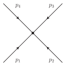
Figure 1: Four-point Feynman rule.

III ONE-LOOP TWO-POINT FUNCTIONS

Using the functional method in momentum space, the generating functional of the scalar field theory with $\phi^{4}$ interactions on the Snyder deformed Euclidean space can be defined Meljanac:2017grw . Considering Figs. 1 and 2, the one-loop two-point function is then given by

$$\begin{split}G_{1-loop}(x_{1},x_{2})=&-\frac{1}{2}\frac{\lambda}{4!}\int\frac{d^{D}p_{1}}{(2\pi)^{D}}\frac{d^{D}p_{2}}{(2\pi)^{D}}\frac{d^{D}\ell}{(2\pi)^{D}}\frac{e^{ip_{1}x_{1}}}{p_{1}^{2}+m^{2}}\frac{e^{ip_{2}x_{2}}}{p_{2}^{2}+m^{2}}\frac{(2\pi)^{D}}{\ell^{2}+m^{2}}\\ &\cdot\sum\limits_{\sigma\in P_{4}}\delta\Big{(}D_{4}\big{(}\sigma\big{(}p_{1},p_{2},\ell,-\ell\big{)}\big{)}\Big{)}\cdot g_{3}\Big{(}\sigma\big{(}p_{1},p_{2},\ell,-\ell\big{)}\Big{)}.\end{split}$$ (12)

The general definitions of $\delta(D_{4}(\sigma(p_{1},p_{2},\ell,-\ell)))$ and $g_{3}(\sigma(p_{1},p_{2},\ell,-\ell))$ are given in Meljanac:2017grw . In particular, $\sigma$ denotes a permutation $P_{4}$ over the momenta in both arguments, respectively. We are going to compute some of them for each of the interactions $S_{1},S_{2}$, and $S_{3}$ in the following subsections.

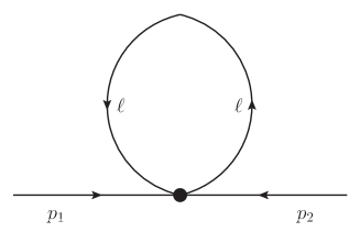
Figure 2: The one-loop tadpole contribution to the two-point function.

III.1 Momentum-conserving integrals

III.1.1 The one-loop two-point function from the action $S_{1}$

Out of 24 $P_{4}$ permutations, we observe that the equation $D_{4}=0$ for the arguments $(p_{1},p_{2},\ell,-\ell)$, $(p_{1},p_{2},-\ell,\ell)$, $(p_{2},p_{1},\ell,-\ell)$, $(p_{2},p_{1},-\ell,\ell)$, $(\ell,-\ell,p_{1},p_{2})$, $(-\ell,\ell,p_{1},p_{2})$, $(\ell,-\ell,p_{2},p_{1})$ and $(-\ell,\ell,p_{2},p_{1})$ admit the same unique solution $p_{1}=-p_{2}$. The remaining sixteen can be shown to be momentum nonconserving by checking the iterative solution to the $\delta$ functions up to the $\beta^{2}$ order. We then work on the Jacobian determinant with respect to $p_{2}$ and the $g_{3}$ factor. For the first four cases we have

$$\det\left(\frac{\partial D_{4_{\mu}}}{\partial p_{2_{\nu}}}\right)\bigg{|}_{p_{2}=-p_{1}}=1,\quad g_{3}=\left(1+\beta\ell^{2}\right)^{-\frac{D+1}{2}},$$ (13)

while, for the others,

$$\begin{split}\det\left(\frac{\partial D_{4_{\mu}}}{\partial p_{2_{\nu}}}\right)\bigg{|}_{p_{2}=-p_{1}}=&\det\left(\frac{\partial D_{\mu}}{\partial q_{\nu}}\right)\bigg{|}_{\stackrel{{\scriptstyle q=0}}{{k=\pm\ell}}}\cdot\det\left(\frac{\partial D_{\mu}}{\partial k_{\nu}}\right)\bigg{|}_{\stackrel{{\scriptstyle q=-k}}{{k=\pm p_{1}}}}\\ =&\det\left(\frac{\partial D_{\mu}}{\partial q_{\nu}}\right)\bigg{|}_{\stackrel{{\scriptstyle q=0}}{{k=\pm\ell}}}\cdot\det\left(\frac{\partial D_{\mu}}{\partial q_{\nu}}\right)\bigg{|}_{\stackrel{{\scriptstyle q=-k}}{{k=\pm p_{1}}}}\\ =&\left(1+\beta\ell^{2}\right)^{\frac{D+1}{2}}\left(1+\beta p_{1}^{2}\right)^{-\frac{D+1}{2}},\\ g_{3}=&\left(1+\beta p_{1}^{2}\right)^{-\frac{D+1}{2}}.\end{split}$$ (14)

Thus all eight integrals take the same form and sum to

$$\begin{split}&-\frac{\lambda}{6}\int\frac{d^{D}p_{1}}{(2\pi)^{D}}\frac{d^{D}p_{2}}{(2\pi)^{D}}\frac{d^{D}\ell}{(2\pi)^{D}}\cdot\frac{e^{ip_{1}x_{1}}}{p_{1}^{2}+m^{2}}\frac{e^{ip_{2}x_{2}}}{p_{2}^{2}+m^{2}}\frac{1}{\left(\ell^{2}+m^{2}\right)\left(1+\beta\ell^{2}\right)^{\frac{D+1}{2}}}.\end{split}$$ (15)

We then extract a universal tadpole integral for the momentum-conserving part of the Snyder two-point function

$$\begin{split}\mathcal{I}_{1}=\int\frac{d^{D}\ell}{(2\pi)^{D}}\frac{1}{\left(\ell^{2}+m^{2}\right)\left(1+\beta\ell^{2}\right)^{\frac{D+1}{2}}}.\end{split}$$ (16)

One can immediately notice that this integral is UV finite in any dimension because of the fast $\mathcal{O}\left(|\ell|^{-(D+1)}\right)$ damping term $(1+\beta\ell^{2})^{-\frac{D+1}{2}}$. For general $D$ the integral can be expressed analytically using hypergeometric functions

$$\mathcal{I}_{1}=(4\pi)^{-\frac{D}{2}}\beta^{1-\frac{D}{2}}\left(\frac{\sqrt{\pi}}{\Gamma\left(\frac{D+1}{2}\right)}\frac{1}{m^{2}\beta}\;{{}_{2}F_{1}}\left(1,\frac{D}{2};\frac{1}{2};\frac{1}{m^{2}\beta}\right)-\frac{(m^{2}\beta)^{\frac{D}{2}-1}}{(m^{2}\beta-1)^{\frac{D+1}{2}}}\frac{\pi}{\Gamma\left(\frac{D}{2}\right)}\right).$$ (17)

Further simplifications occur for specific values of $D$. When $D=4$,

$$\mathcal{I}_{1}\Big{|}_{D=4}=\frac{1}{(4\pi)^{2}\beta}\frac{2}{3}\left(\frac{1+2m^{2}\beta}{(1-m^{2}\beta)^{2}}-\frac{3m^{2}\beta}{\sqrt{(m^{2}\beta-1)^{5}}}\sec^{-1}\sqrt{m^{2}\beta}\right),$$ (18)

and when $D=3$

$$\mathcal{I}_{1}\Big{|}_{D=3}=\frac{1}{8\pi\sqrt{\beta}}\frac{1}{(1+m\sqrt{\beta})^{2}}.$$ (19)

III.1.2 The one-loop two-point function from the action $S_{2}$

We now move from $S_{1}$ to $S_{2}$. There are again eight momentum-conserving permutations for $S_{2}$: they are $(p_{1},\ell,-\ell,p_{2})$, $(p_{1},-\ell,\ell,p_{2})$, $(p_{2},\ell,-\ell,p_{1})$, $(p_{2},-\ell,\ell,p_{1})$, $(\ell,p_{1},p_{2},-\ell)$, $(-\ell,p_{1},p_{2},\ell)$, $(\ell,p_{2},p_{1},-\ell)$ and $(-\ell,p_{2},p_{1},\ell)$. The first four of them have Jacobian equal to one and $g_{3}=(1+\beta\ell^{2})^{-\frac{D+1}{2}}$, while the others satisfy

$$\begin{split}\det\left(\frac{\partial D_{4_{\mu}}}{\partial p_{2_{\nu}}}\right)\bigg{|}_{p_{2}=-p_{1}}=&\det\left(\frac{\partial D_{\mu}}{\partial k_{\nu}}\right)\bigg{|}_{\stackrel{{\scriptstyle k=0}}{{q=\pm\ell}}}\cdot\det\left(\frac{\partial D_{\mu}}{\partial k_{\nu}}\right)\bigg{|}_{\stackrel{{\scriptstyle k=-q}}{{q=\mp p_{1}}}}\\ =&\det\left(\frac{\partial D_{\mu}}{\partial k_{\nu}}\right)\bigg{|}_{\stackrel{{\scriptstyle k=0}}{{q=\pm\ell}}}\cdot\det\left(\frac{\partial D_{\mu}}{\partial q_{\nu}}\right)\bigg{|}_{\stackrel{{\scriptstyle k=-q}}{{q=\mp p_{1}}}}\\ =&\left(1+\beta\ell^{2}\right)\left(1+\beta p_{1}^{2}\right)^{-\frac{D+1}{2}},\\ g_{3}=&(1+\beta p_{1}^{2})^{-\frac{D+1}{2}}.\end{split}$$ (20)

We then have a second type of tadpole integral

$$\mathcal{I}_{2}=\int\frac{d^{D}\ell}{(2\pi)^{D}}\frac{1}{(\ell^{2}+m^{2})(1+\beta\ell^{2})},$$ (21)

which converges only when $D<4$. This integral can nevertheless be evaluated using the standard dimensional regularization prescription

$$\begin{split}\mathcal{I}_{2}=&\int\frac{d^{D}\ell}{(2\pi)^{D}}\frac{1}{(\ell^{2}+m^{2})(1+\beta\ell^{2})}=\beta^{1-\frac{D}{2}}\int\frac{d^{D}\ell}{(2\pi)^{D}}\frac{1}{(\ell^{2}+\beta m^{2})(1+\ell^{2})}\\ =&\beta^{1-\frac{D}{2}}\frac{\Gamma\left(2-\frac{D}{2}\right)}{(4\pi)^{\frac{D}{2}}}\int\limits_{0}^{1}dx\,\Big{(}1-x\big{(}1-\beta m^{2}\big{)}\Big{)}^{\frac{D}{2}-2}=-\beta^{1-\frac{D}{2}}\;\frac{\Gamma\left(1-\frac{D}{2}\right)}{(4\pi)^{\frac{D}{2}}}\;\frac{1-(\beta m^{2})^{\frac{D}{2}-1}}{1-\beta m^{2}}.\end{split}$$ (22)

In the $D\to 4-\epsilon$ limit this integral reduces to

$$\mathcal{I}_{2}\Big{|}_{D\to 4-\epsilon} = \frac{1}{(4\pi)^{2}\beta}\left(\frac{2}{\epsilon}+1-\gamma_{E}+\ln(4\pi\beta)+\frac{m^{2}\beta}{1-m^{2}\beta}\ln\big{(}m^{2}\beta\big{)}\right)+\mathcal{O}(\epsilon).$$ (23)

On the other hand, when $D=3$, $\mathcal{I}_{2}$ takes a simple finite value

$$\mathcal{I}_{2}\Big{|}_{D=3}=\frac{1}{4\pi\sqrt{\beta}}\frac{1}{1+m\sqrt{\beta}},$$ (24)

which is regularization independent.

III.1.3 The one-loop two-point function from the action $S_{3}$

An even more complicated situation occurs with the third term of the interaction (11). There we have 16 different momentum-conserving permutations. Twelve of them take the same form as $\mathcal{I}_{1}$. There are four other momentum-conserving permutations $(p_{1},\ell,p_{2},-\ell)$, $(p_{1},-\ell,p_{2},\ell)$, $(p_{2},\ell,p_{1},-\ell)$ and $(p_{2},\ell,p_{1},-\ell)$ which are different, because the determinant $\det\left(\frac{\partial D_{\mu}}{\partial k_{\nu}}\right)$ must be evaluated at a general point $\left(k=\pm p,q=\pm\ell\right)$ with $p$ being an external momentum, as shown in Appendix A. The result leads to the following loop integral

$$\begin{split}\mathcal{I}_{3}=&\int\frac{d^{D}\ell}{(2\pi)^{D}}\frac{1}{(\ell^{2}+m^{2})(1+\beta\ell^{2})}\left(1-\frac{\beta p\cdot\ell}{1+\sqrt{1+\beta p^{2}}}\right)^{1-D}.\end{split}$$ (25)

This integral can be evaluated using dimensional regularization techniques, as demonstrated in Appendix B. The result clearly shows that there is no $1/\epsilon$ UV divergence in the $D\to 4$ limit; however, a logarithmic IR divergent term $\ln\big{(}\beta p^{2}\big{)}$ does emerge in the same limit. Since taking away the last, momentum dependent factor from (25) simply turns $\mathcal{I}_{3}$ back to $\mathcal{I}_{2}$, we conclude that an effect of this factor is to turn the UV divergence in $\mathcal{I}_{2}$ into an IR divergence, or, in other words, to induce UV/IR mixing.

III.2 Momentum nonconserving integrals

III.2.1 General considerations of the momentum nonconserving integral

In previous subsections III.A1, III.A2, and III.A3, we have only considered the momentum-conserving integrals $\mathcal{I}_{1}$, $\mathcal{I}_{2}$, and $\mathcal{I}_{3}$, respectively. There are, as already discussed in Meljanac:2017grw and in the prior parts of this article, a number of momentum nonconserving ones as well. Unlike the momentum-conserving integrals, we do not have explicit integrated expression for such integrals. Nevertheless, we shall presently discuss certain of their properties which may be accessible without full integration.

Before we start our technical discussion it is also worthy to mentioning that momentum nonconservation, causing loss of translation invariance, could be a much more fundamental issue regarding certain basis of quantum field theory, which we are not going to study in this article. Instead we follow the prescription in Meljanac:2017grw to eliminate the deformed $\delta$ functions in (12) by an integration over one fixed external momentum, here $p_{2}$, i.e., making it a function of $(p_{1},\ell)$: $p_{2}^{\sigma}(p_{1},\ell)$ with $\sigma$ permutations. The to-be-evaluated loop integral would formally bear the following form:

$$\begin{split}G_{1-loop}(x_{1},x_{2})=&-\frac{1}{2}\frac{\lambda}{4!}\int\frac{d^{D}p_{1}}{(2\pi)^{D}}\frac{d^{D}\ell}{(2\pi)^{D}}\\ &\cdot\frac{e^{ip_{1}x_{1}}}{p_{1}^{2}+m^{2}}\frac{1}{\ell^{2}+m^{2}}\cdot\sum\limits_{\sigma\in P_{4}}\frac{e^{ip_{2}^{\sigma}(p_{1},\ell)x_{2}}}{p_{2}^{\sigma}(p_{1},\ell)^{2}+m^{2}}g_{3}\Big{(}\sigma\big{(}p_{1},p_{2}^{\sigma}(p_{1},\ell),\ell,-\ell\big{)}\Big{)}\left(\frac{\delta D_{4}}{\delta p_{2}}\right)^{-1}.\end{split}$$ (26)

At this point, the remaining task is to solve each of the $\sigma$-permuted functions $p_{2}^{\sigma}(p_{1},\ell)$ explicitly, which is not really easy though. What one could try is to use the fact that star product (4) contains only vector objects (vectors and scalar products), therefore it could be convenient to project $\ell$ and $p_{2}$ momenta to the external moment $p_{1}$ component and to the perpendicular component $\ell_{\perp}$ of loop moment $\ell$, making it $\ell=(xp_{1},\ell_{\perp})$, and set up a simple ansatz for $p_{2}$ as: $p_{2}=f_{1}(x,p_{1},\ell_{\perp})p_{1}+f_{2}(x,p_{1},\ell_{\perp})\ell_{\perp}$. With this setting the Snyder-deformed momentum conservation in one-loop two-point function becomes a set of algebraic equations with respect to $f_{1}$ and $f_{2}$, respectively.

III.2.2 Superficial UV divergence of the momentum nonconserving integral

As an example, we study the nonconserving integral with modified $\delta$ function $\delta(D\left(p_{2},-\ell)+D(\ell,p_{1})\right)$ coming from $S_{3}$ term (10). In this case the momentum $p_{2}$ is not equal to $-p_{1}$ from Fig.2, and the difference starts at $\beta^{1}$ order. The relevant integral is given below:

$$I=\int\frac{d^{D}\ell}{(2\pi)^{D}}\frac{1}{\ell^{2}+m^{2}}\frac{e^{ip_{2}x_{2}}}{p_{2}^{2}+m^{2}}\frac{1}{1+\beta\ell^{2}}\left(1+\frac{\beta\ell\cdot p_{2}}{1+\sqrt{1+\beta p_{2}^{2}}}\right)^{1-D}\left(\frac{1+\beta\ell\cdot p_{2}}{1-\beta\ell\cdot p_{1}}\right)^{\frac{D+1}{2}},$$ (27)

where defining an equation for $p_{2}$, in accordance to the ansatz setup,

$$p_{2}^{\sigma}(p_{1},\ell)=f^{\sigma}_{1}(x,\ell_{\perp},p_{1})p_{1}+f^{\sigma}_{2}(x,\ell_{\perp},p_{1})\ell_{\perp},\;\forall\sigma\in P_{4}-{\rm permutations},$$ (28)

is resolved by using the Snyder momentum addition relations (7)

$$D_{\mu}(p_{2},-\ell)=-D_{\mu}(\ell,p_{1}).$$ (29)

The above simple equation (29) then, after using (28), transfers into two complicated algebraic relations for, generically $f_{1}$ and $f_{2}$, respectively,

$$\frac{1}{1+\beta(xf_{1}p_{1}^{2}+f_{2}\ell_{\perp}^{2})}\left(f_{1}-x+\frac{\beta\ell_{\perp}^{2}(f_{1}f_{2}-f_{2}^{2})}{1+\sqrt{1+\beta(f_{1}^{2}p_{1}^{2}+f_{2}^{2}\ell_{\perp}^{2})}}\right)=-\frac{1}{1-x\beta p_{1}^{2}}\left(1+x+\frac{\beta\ell_{\perp}^{2}}{1+\sqrt{1+\beta(x^{2}p_{1}^{2}+\ell_{\perp})}}\right),$$ (30)

$$\frac{1}{1+\beta(xf_{1}p_{1}^{2}+f_{2}\ell_{\perp}^{2})}\left(f_{2}-1+\frac{\beta p_{1}^{2}(xf_{1}f_{2}-f_{1}^{2})}{1+\sqrt{1+\beta(f_{1}^{2}p_{1}^{2}+f_{2}^{2}\ell_{\perp}^{2})}}\right)=-\frac{1}{1-x\beta p_{1}^{2}}\left(1-\frac{x\beta p_{1}^{2}}{1+\sqrt{1+\beta(x^{2}p_{1}^{2}+\ell_{\perp})}}\right).$$ (31)

While it is hard to obtain closed form solution for $f_{1}$ and $f_{2}$ from these two equations, one can use them to analyze the large $|\ell|$ behavior of $f_{1}$ and $f_{2}$ by realizing that $x\sim\ell_{\perp}\sim|\ell|^{1}$. Using an ansatz $f_{i}\sim|\ell|^{k_{i}}$ for large $|\ell|$, we find that $k_{1}=1$ and $k_{2}=0$, i.e., $p_{2}\sim|\ell|^{1}$. Using this scaling we find that (27) is superficially UV finite for $D<9$. Thus the integral (27) is superficially UV finite at four dimensions.

Finally full solutions, if obtainable, are lengthy and yet the analytical solution to the integration over $\ell$ in (27) is still at large. We hope such integral could be solved in near future.

IV UV/IR mixing

Generally speaking, when a UV-divergent loop integral is regularized by deformation, turning off the deformation would lead to divergences in the commutative limit at the quantum level. For example, in the Moyal $\phi^{4}$ theory, the nonplanar/regularized integral of the two-point function reads

$$I(p,\theta)=\int\frac{d^{D}\ell}{(2\pi)^{D}}\frac{e^{-\frac{1}{2}{\ell_{\mu}\theta^{\mu\nu}p_{\nu}}}}{\ell^{2}+m^{2}}.$$ (32)

When either $\theta$ or $p$ goes to zero in the integrand, this integral becomes the UV divergent commutative tadpole

$$I(p,0)=I(0,\theta)=\int\frac{d^{D}\ell}{(2\pi)^{D}}\frac{1}{\ell^{2}+m^{2}}.$$ (33)

For this reason one expects that the integral $I(p,\theta)$ would exhibit a $(\theta p)$-dependent divergence, which was indeed found Minwalla:1999px .

A more careful look at the discussion above forces us to conclude that we are here actually considering two divergences, $\theta\to 0$ and $p\to 0$. The first divergence, occurring at the commutative limit $\theta\to 0$, is less surprising since an UV divergence is already present in the undeformed theory. So, this limit could be simply interpreted as a recovery.

The second divergence $p\to 0$ is more intriguing. It shifts the UV divergence in the commutative/undeformed theory to the IR regime ($p\to 0$), which is a big modification to the quantum field theory, and leads to the (in-)famous UV/IR mixing. It is not hard to see that the reason why these two divergences become associated with each other in the Moyal theory is the regulator momentum dependence, which is a consequence of the tensorial nature of the Moyal deformation parameter $\theta^{\mu\nu}$.

Now we move from Moyal to the Snyder $\phi^{4}$ theory. First we consider the same vanishing external momentum limit of (12). Since such a limit brings (32) to (33), it could be considered as an indicator of the UV behavior without momentum-dependent regularization. Using (7) it is not hard to find that, in the limit of vanishing external momenta and for any normalized combination of $c_{1}$, $c_{2}$, and $c_{3}$, the integrand of (12) satisfies the following relation

$$\begin{split}\lim\limits_{p_{1}\to 0}-\frac{1}{2}\frac{\lambda}{4!}&\int{(2\pi)^{D}}\frac{d^{D}p_{2}}{(2\pi)^{D}}\frac{d^{D}\ell}{(2\pi)^{D}}\frac{e^{ip_{1}x_{1}}}{p_{1}^{2}+m^{2}}\frac{e^{ip_{2}x_{2}}}{p_{2}^{2}+m^{2}}\frac{(2\pi)^{4}}{\ell^{2}+m^{2}}\\ &\cdot\sum\limits_{\sigma\in P_{4}}\delta\Big{(}D_{4}\big{(}\sigma\big{(}p_{1},p_{2},\ell,-\ell\big{)}\big{)}\Big{)}\cdot g_{3}\Big{(}\sigma\big{(}p_{1},p_{2},\ell,-\ell\big{)}\Big{)}\sim-\frac{\lambda}{6}\big{(}2\mathcal{I}_{1}+\mathcal{I}_{2}\big{)}.\end{split}$$ (34)

In other words the $4!=24$ momentum permutations reduce to only two types: 16 $\mathcal{I}_{1}$ and 8 $\mathcal{I}_{2}$, respectively. Therefore, the zero-momentum limit is UV divergent because of the $\mathcal{I}_{2}$ integral. However, $\mathcal{I}_{2}$ is, unlike the Moyal theory, regulated from the commutative quadratic to logarithmic UV divergences. From this observation we conclude that the commutative and IR limits discussed above become independent from each other in Snyder theory, since the Snyder deformation parameter $\beta$ is a scalar. The $\beta\to 0$ limit of the integrals $\mathcal{I}_{1}$ and $\mathcal{I}_{2}$ is divergent, which is the expected recovery of the divergence of the commutative theory.

Next we turn to the momentum dependence of the Snyder one-loop two-point functions. We have only computed one part of it as the integral $\mathcal{I}_{3}$. When $D\geq 4$, this integral is superficially UV finite only when the external momentum $p\neq 0$, and therefore it can exhibit an infrared divergence when $p\to 0$. Indeed, once we evaluate $\mathcal{I}_{3}$ properly, we find in the limit $p\to 0$,

$$\mathcal{I}_{3}\,\bigg{|}_{\hskip 1.42262pt{\begin{subarray}{c}D=4\\ p\to 0\end{subarray}}}\;\sim\;-\frac{1}{(4\pi)^{2}\beta}\ln\big{(}-\beta p^{2}\big{)},$$ (35)

and hence a $\ln p^{2}$ divergence when $p\to 0$. (See Appendix B for more details.) This UV/IR mixing may be considered as a new type induced by nonassociativity in comparison with the Moyal $\phi^{4}$ theory, since the corresponding UV divergence is of the $\mathcal{I}_{2}$ type, i.e. already regulated by the Snyder deformation when compared with the commutative theory, while the additional momentum-dependent regulator in $\mathcal{I}_{3}$ (25) comes as a consequence of the nonassociativity of the Snyder star product.

More generally speaking, the full four-dimensional Snyder one-loop two-point function, including the momentum nonconserving integrals, depends on the external momentum. Although we do not know explicitly the results of the momentum nonconserving integrals, we do know that when taking the external momentum zero limit at the integrand level, part of them, for example (27) discussed in Sec. III.B.2., becomes the UV divergent integral $\mathcal{I}_{2}$ (21) in accord with the aforementioned universal zero-momentum limit (34). On the other hand, when $p=p_{1}\neq 0$, this integral exhibits a superficially finite UV power counting divergence as shown in Sec. III.B.2., so we may qualitatively conclude that (some of) those integrals in the full one-loop two-point function, which converge to $\mathcal{I}_{2}$ in the $p\to 0$ limit, would exhibit IR divergence in 4D if they are finite, at finite nonzero value of the momentum $p$. Therefore, we consider UV/IR mixing as a general property of the Snyder one-loop two-point function.

V Discussions

Before concluding the article, it is worth noting that a variant of our model exists for $\beta<0$ Mignemi:2011gr . In such a case, the momenta are bounded by $p^{2}<1/\beta$ and the integrals run over a finite range. We can express the external momentum-independent integrals $\mathcal{I}_{1}$ and $\mathcal{I}_{2}$ in this case by introducing the adimensional loop momenta $L^{\mu}=\sqrt{|\beta|}\ell^{\mu}$. The integrals then run from $L=|L^{\mu}|=0$ to $L=1$. It is not hard to show that in this setting $\mathcal{I}_{2}$ reduces to the following expression

$$\mathcal{I}_{2}=\frac{2\beta}{\Gamma\left(\frac{D}{2}\right)}(4\pi\beta)^{-\frac{D}{2}}\int\limits_{0}^{1}dL\,\frac{L^{D-1}}{(L^{2}+m^{2})(1-L^{2})}.$$ (36)

The integral above is divergent at its upper limit for any $D$, and therefore it is not regularizable by dimensional regularization. Similarly, $\mathcal{I}_{1}$ becomes

$$\mathcal{I}_{1}=\frac{2\beta}{\Gamma\left(\frac{D}{2}\right)}(4\pi\beta)^{-\frac{D}{2}}\int\limits_{0}^{1}dL\,\frac{L^{D-1}}{(L^{2}+m^{2})(1-L^{2})^{\frac{D+1}{2}}}.$$ (37)

This integral is still superficially divergent at the upper limit, and one can only assign it a dimensionally regularized value in terms of the Gauss hypergeometric function:

$$\mathcal{I}_{1}=\frac{\Gamma\left(\frac{1-D}{2}\right)\Gamma\left(\frac{D}{2}\right)}{2m^{2}\Gamma\left(\frac{1}{2}\right)}\,_{2}F_{1}\left(1,\frac{D}{2};\frac{1}{2};\frac{-1}{m^{2}}\right).$$ (38)

This expression is finite for even dimensions, but divergent for odd dimensions as $\Gamma\left(\frac{1-D}{2}\right)$. Technically, the complicated divergences we have encountered in this section are not surprising as the cutoff at $L=1$ still leaves the same pole at the upper boundary of the integral. It appears that the negative $\beta$ case could be more difficult to handle at loop level than positive $\beta$. Thus we leave this issue for future investigation.

Another technical possibility is to define and compute an analogue to the Coleman-Weinberg effective potential Coleman:1973jx by using the same zero external momentum limit integrand in Eq. (34), which yields

$$\begin{split}V_{\rm eff}(\varphi)=\frac{\lambda}{4!}\varphi^{4}+\beta^{-\frac{D}{2}}\int\frac{d^{D}\ell}{(2\pi)^{D}}\frac{1}{2}\sum\limits_{n=1}^{\infty}\frac{(-1)^{n+1}}{n}\Bigg{(}\frac{\beta\lambda\varphi^{2}}{6\ell^{2}(1+\ell^{2})}\bigg{(}1+\frac{2}{(1+\ell^{2})^{\frac{D-1}{2}}}\bigg{)}\Bigg{)}^{n}\\ =\frac{\lambda}{4!}\varphi^{4}+\frac{1}{2}\beta^{-\frac{D}{2}}\int\frac{d^{D}\ell}{(2\pi)^{D}}\ln\Bigg{(}1+\frac{\beta\lambda\varphi^{2}}{6\ell^{2}(1+\ell^{2})}\bigg{(}1+\frac{2}{(1+\ell^{2})^{\frac{D-1}{2}}}\bigg{)}\Bigg{)},\end{split}$$ (39)

where $\varphi$ denotes the constant-valued field in the zero-momentum limit.

As already suggested by (16) and (21), the above loop integral (39) is finite and computable for $D=3$, giving

$$V_{\rm eff}(\varphi)\Big{|}_{D=3}=\frac{\lambda}{4!}\varphi^{4}+\frac{1}{12\pi^{2}\sqrt{\beta^{3}}}\bigg{(}2\pi-\sum\limits_{i=1}^{6}f(x_{i})\bigg{)},$$ (40)

where

$$f(x)=\frac{2(a-1)x^{4}+(7a-2)x^{2}-6a}{3x^{5}+4x^{3}+(1+a)x}\ln(-x),\quad a=\frac{1}{6}\beta\lambda\varphi^{2},$$ (41)

and $x_{1,2,...,6}$ are the solutions to the sixth-order polynomial equation

$$x^{6}+2x^{4}+(1+a)x^{2}+3a=0.$$ (42)

Once we analyze (40) numerically, it is not hard to find out that the aforementioned $\beta\to 0$ divergence could be considered as enhancing the one-loop contribution against the tree level at small $\beta$ values, as illustrated in Fig. 3.

Figure 3: The one-loop corrected effective potential of Snyder deformed three-dimensional $\phi^{4}$ theories for $\lambda=0.1$ and $\beta=0.001$ (solid line), $\lambda=\beta=0.1$ (dashed line) and the tree level effective potential for $\lambda=0.1$ (dotted line). The smaller $\beta$ value clearly increases the deviation from the tree level value. One may also notice that unlike the commutative theory Peskin:1995ev , no artificial new minima emerge despite large loop correction.

In general, large loop corrections suggest that certain nonperturbative effects may occur Peskin:1995ev . One natural question is then whether it is possible to follow the Wilson-Fisher $4-\epsilon$ analysis Wilson:1971dc ; Glimm:1987ng ; Kleinert:2001ax instead of going naively to dimension three, as the Wilson-Fisher approach is long proven to be correct in extracting the critical behavior of $\phi^{4}$ and related theories in lower dimensions. Besides the large perturbation issue, this procedure is not yet possible since we do not really know how to define the wave function renormalization without the full two-point function solution. One may, however, notice two properties if we choose to use the zero-momentum limit at integrand level as in the naive effective potential analysis above. First, the four field vertex at zero-momentum limit, i.e., the second term of the sum in the first line for (39), remains finite when $D\to 4$. Also, the UV divergence in (23), when compared with usual mass renormalization, receives its corresponding mass dimension via $\beta^{-1}$ instead of $m^{2}$. One may wander how such modification would affect the usual renormalization group analysis. All these observations seem to hint that Snyder deformed $\phi^{4}$ theory could possess more complicated quantum behavior than the UV/IR mixing analyzed in the prior sections and require analysis beyond the fixed order loop calculations too.

VI Conclusions

In this article we have studied the effect of Hermitian realization of the nonassociative and noncommutative Snyder deformation of the scalar $\phi^{4}$ quantum field theory, by computing tadpole diagram contribution to the one-loop two-point function. We have shown that the nonassociativity increases the number of different possible terms in the action with respect to the associative case and affects the results at the quantum level.

We have calculated the momentum-conserving tadpole integrals for the three different inequivalent terms $S_{1}$, $S_{2}$ and $S_{3}$ that can appear in the general $\beta$-exact Snyder $\phi^{4}$ interaction (11). They are found to possess remarkably different properties. Of the three integrals $\mathcal{I}_{1}$, $\mathcal{I}_{2}$ and $\mathcal{I}_{3}$ coming from the three terms $S_{1}$, $S_{2}$ and $S_{3}$, $\mathcal{I}_{1}$ is finite in all dimensions, $\mathcal{I}_{2}$ is finite when $D<4$ but logarithmically divergent when $D=4$, whereas $\mathcal{I}_{3}$ is finite for finite momentum, yet exhibits a logarithmic IR divergence when $p\to 0$ in the $D=4$ case.

The integrals $\mathcal{I}_{1},\mathcal{I}_{2}$ and $\mathcal{I}_{3}$ exhibit uniform divergent behavior in the commutative limit when $\beta\to 0$, as expected. On the other hand, their infrared limits can be quite different: $\mathcal{I}_{1}$ and $\mathcal{I}_{2}$ are independent of external momentum, and therefore remain unchanged in the IR limit. However, $\mathcal{I}_{3}$ is momentum dependent and exhibits a logarithmic infrared divergence when $D=4$. The logarithmic IR divergence of $\mathcal{I}_{3}$ matches the logarithmic UV divergence of $\mathcal{I}_{2}$ at $D\to 4$, which, at the integrand level, is exactly the $p\to 0$ limit of $\mathcal{I}_{3}$. For this reason we conclude that a new type of UV/IR mixing, induced by nonassociativity on top of noncommutativity, occurs in $\mathcal{I}_{3}$ and represents a general quantum feature of Snyder deformed scalar $\phi^{4}$ field theory at the level of the one-loop two-point function. We also extend our analysis on UV/IR mixing into the momentum nonconserving integrals (26) by obtaining through UV power counting as qualitative evidence that UV/IR mixing also emerge in momentum nonconserving integrals and therefore should be considered as a general property of the Snyder $\phi^{4}$ quantum field theory.

At present, the problem of computing complete momentum non-conserving parts of the two-point functions is still open. The method presented in Sec III.B. does allow us to integrate over deformed $\delta$ functions explicitly or implicitly, as well as to analyze certain properties of the loop integrand by using the UV power counting. Yet any analytical solution in closed form of the final integration over the loop momentum is still too far to reach. It is without a doubt that knowing some of such solutions would efficiently improve our overall understanding of the one-loop quantum properties of Snyder $\phi^{4}$ theory. However many questions, both practical ones (like what would be the total sum of UV/IR mixing terms, and/or whether certain cancellation mechanism for UV/IR mixing could emerge), and conceptual ones (like whether the full one-loop corrected two-point function can bear sound meaning as a QFT), unfortunately still remain unanswered. Anyway, we hope that some of the above issues could be settled in the future.

While the full one-loop two-point function is not yet available, its zero-momentum limit at integrand level can be defined completely. We exploited this fact discussing an analogue of the Coleman-Weinberg effective potential, noticing that finite one-loop results can be obtained analytically for the three-dimensional theory. Also the UV divergence is clearly reduced when $D=4$. The loop correction tends to diverge when $\beta\to 0$ and therefore could become large when $\beta$ is small. We consider these findings as suggestions towards nonperturbative studies on the Snyder $\phi^{4}$ theory.

VII Acknowledgments

This work is supported by the Croatian Science Foundation (HRZZ) under Contract No. IP-2014-09-9582. We acknowledge the support of the COST Action MP1405 (QSPACE). S. M. and J. Y. acknowledges support by the H2020 Twining project No. 692194, RBI-T-WINNING. S. M. acknowledges the support from ESI and COST, from his participation to the workshop ”Noncommutative geometry and gravity” and wishes to thank H. Grosse for a discussion. J. T. and J. Y. would like to acknowledge the support of W. Hollik and the Max-Planck-Institute for Physics, Munich, for hospitality, as well as C. P. Martin and P. Schupp for discussions. Also J. T. would like to thank E. Seiler for useful discussions, and V. G. Kupriyanov and D. Lust for useful discussions and pointing new Refs. Hohm:2017cey ; Hohm:2017pnh to us.

Appendix A THE DETERMINANTS

We present here an evaluation for the determinants $\det\left(\frac{\partial D_{\mu}}{\partial k_{\nu}}\right)$ and $\det\left(\frac{\partial D_{\mu}}{\partial q_{\nu}}\right)$. We start with an ansatz for $D_{\mu}(k,q)$, which contains only scalar and vector objects but not pseudovectors and pseudoscalars, i.e.

$$D_{\mu}(k,q)=f\left(k^{2},k\cdot q,q^{2}\right)k_{\mu}+g\left(k^{2},k\cdot q,q^{2}\right)q_{\mu}.$$ (43)

It is then easy to find that

$$\begin{split}\frac{\partial D_{\mu}}{\partial k_{\nu}}=&\delta^{\nu}_{\mu}f\left(k^{2},k\cdot q,q^{2}\right)\\ &+k_{\mu}(2k^{\nu}f^{(1,0,0)}\left(k^{2},k\cdot q,q^{2}\right)+q^{\nu}f^{(0,1,0)}\left(k^{2},k\cdot q,q^{2}\right))\\ &+q_{\mu}(2k^{\nu}g^{(1,0,0)}\left(k^{2},k\cdot q,q^{2}\right)+q^{\nu}g^{(0,1,0)}\left(k^{2},k\cdot q,q^{2}\right)),\end{split}$$ (44)

$$\begin{split}\frac{\partial D_{\mu}}{\partial q_{\nu}}=&\delta^{\nu}_{\mu}g\left(k^{2},k\cdot q,q^{2}\right)\\ &+q_{\mu}(k^{\nu}g^{(0,1,0)}\left(k^{2},k\cdot q,q^{2}\right)+2q^{\nu}g^{(0,0,1)}\left(k^{2},k\cdot q,q^{2}\right))\\ &+k_{\mu}(k^{\nu}f^{(0,1,0)}\left(k^{2},k\cdot q,q^{2}\right)+2q^{\nu}f^{(0,0,1)}\left(k^{2},k\cdot q,q^{2}\right)),\end{split}$$ (45)

where $f^{(1,0,0)}(x,y,z)=\frac{\partial}{\partial x}f(x,y,z)$, $f^{(0,1,0)}(x,y,z)=\frac{\partial}{\partial y}f(x,y,z)$ and $f^{(0,0,1)}(x,y,z)=\frac{\partial}{\partial z}f(x,y,z)$.

Now, using the Sylvester’s determinant identity

$$\det(I_{m}+AB)=\det(I_{n}+BA),$$ (46)

one can show that

$$\det\left(\delta_{\mu}^{\nu}+a_{1_{\mu}}b_{1}^{\nu}+a_{2_{\mu}}b_{2}^{\nu}\right)=1+a_{1}\cdot b_{1}+a_{2}\cdot b_{2}+(a_{1}\cdot b_{1})(a_{2}\cdot b_{2})-(a_{1}\cdot b_{2})(a_{2}\cdot b_{1}).$$ (47)

Therefore

$$\begin{split}\det\left(\frac{\partial D_{\mu}}{\partial k_{\nu}}\right)=&f^{D}\Big{(}1+f^{-1}\left(2k^{2}f^{(1,0,0)}+k\cdot q(f^{(0,1,0)}+2g^{(1,0,0)})+q^{2}g^{(0,1,0)}\right)\\ &+2f^{-2}\left(k^{2}q^{2}-(k\cdot q)^{2}\right)\left(f^{(1,0,0)}g^{(0,1,0)}-g^{(1,0,0)}f^{(0,1,0)}\right)\Big{)},\end{split}$$ (48)

$$\begin{split}\det\left(\frac{\partial D_{\mu}}{\partial q_{\nu}}\right)=&g^{D}\Big{(}1+g^{-1}\left(k^{2}f^{(0,1,0)}+k\cdot q(g^{(0,1,0)}+2f^{(0,0,1)})+2q^{2}g^{(0,0,1)}\right)\\ &+2g^{-2}\left(k^{2}q^{2}-(k\cdot q)^{2}\right)\left(g^{(0,0,1)}f^{(0,1,0)}-f^{(0,0,1)}g^{(0,1,0)}\right)\Big{)}.\end{split}$$ (49)

Finally we insert the Snyder realization (5), and after some algebra we get

$$\det\left(\frac{\partial D_{\mu}}{\partial k_{\nu}}\right)=\frac{1+\beta q^{2}}{(1-\beta k\cdot q)^{D+1}}\left(1-\frac{\beta k\cdot q}{1+\sqrt{1+\beta k^{2}}}\right)^{D-1},$$ (50)

and

$$\det\left(\frac{\partial D_{\mu}}{\partial q_{\nu}}\right)=\frac{(1+\beta k^{2})^{\frac{D+1}{2}}}{(1-\beta k\cdot q)^{D+1}}.$$ (51)

We list few special values of these two determinants which are relevant for the calculation in the main text:

$$\begin{split}&k=0{\;\;\>}:\;\det\left(\frac{\partial D_{\mu}}{\partial k_{\nu}}\right)=1+\beta q^{2},\;\det\left(\frac{\partial D_{\mu}}{\partial q_{\nu}}\right)=1,\\ &q=0{\;\;\>}:\;\det\left(\frac{\partial D_{\mu}}{\partial k_{\nu}}\right)=1,\;\det\left(\frac{\partial D_{\mu}}{\partial q_{\nu}}\right)=(1+\beta k^{2})^{\frac{D+1}{2}},\\ &k=-q:\;\det\left(\frac{\partial D_{\mu}}{\partial k_{\nu}}\right)=\det\left(\frac{\partial D_{\mu}}{\partial q_{\nu}}\right)=(1+\beta k^{2})^{-\frac{D+1}{2}}.\end{split}$$ (52)

Appendix B DIMENSIONAL REGULARIZATION OF $\mathcal{I}_{3}$

In this section we present the detailed evaluation of (25). We start by rescaling the mass and momenta with respect to $\beta$:

$$L=\ell\sqrt{\beta},\;P=p\sqrt{\beta},\;M=m\sqrt{\beta}.$$ (53)

Then, after a further redefinition $\mathcal{P}=\frac{P}{1+\sqrt{1+P^{2}}}$, (25) reduces to

$$\begin{split}\mathcal{I}_{3}=&\beta^{1-\frac{D}{2}}\int\frac{d^{D}L}{(2\pi)^{D}}\frac{1}{(L^{2}+M^{2})(1+L^{2})}\left(1-\mathcal{P}\cdot L\right)^{1-D}.\end{split}$$ (54)

The integrand can then be parametrized by two parameters, one for the $L$-quadratic factors while the other for the $L$-linear factor, i.e.

$$\begin{split}\mathcal{I}_{3}=&\beta^{1-\frac{D}{2}}\int\limits_{0}^{1}dx\,\int\limits_{0}^{\infty}dy\,\frac{\Gamma\left(D+1\right)}{\Gamma\left(D-1\right)}\int\frac{d^{D}L}{(2\pi)^{D}}\frac{y^{D-2}}{\left(L^{2}+1+x(M^{2}-1)+y-y\mathcal{P}\cdot L\right)^{D+1}}.\end{split}$$ (55)

It is then straightforward to integrate over $L$ using the (Schwinger) $\alpha$ parametrization

$$\begin{split}\mathcal{I}_{3}=&\frac{\beta^{1-\frac{D}{2}}}{\Gamma\left(D-1\right)}\int\limits_{0}^{1}dx\,\int\limits_{0}^{\infty}dy\,\int\limits_{0}^{\infty}d\alpha\int\frac{d^{D}L}{(2\pi)^{D}}y^{D-2}\,\alpha^{D}\\ &\exp\left[-\alpha\left(\left(L-\frac{y}{2}\mathcal{P}\right)^{2}+x(M^{2}-1)+1+y-y^{2}\frac{\mathcal{P}^{2}}{4}\right)\right]\\ =&\frac{\beta(4\pi\beta)^{-\frac{D}{2}}}{\Gamma\left(D-1\right)}\int\limits_{0}^{1}dx\,\int\limits_{0}^{\infty}dy\,\int\limits_{0}^{\infty}d\alpha\,y^{D-2}\alpha^{\frac{D}{2}}\exp\left[-\alpha\left(x(M^{2}-1)+1+y-y^{2}\frac{\mathcal{P}^{2}}{4}\right)\right]\\ =&\beta(4\pi\beta)^{-\frac{D}{2}}\frac{\Gamma\left(\frac{D}{2}+1\right)}{\Gamma\left(D-1\right)}\int\limits_{0}^{1}dx\,\int\limits_{0}^{\infty}dy\,y^{D-2}\left(x(M^{2}-1)+1+y-y^{2}\frac{\mathcal{P}^{2}}{4}\right)^{-1-\frac{D}{2}}\\ =&\beta(4\pi\beta)^{-\frac{D}{2}}\frac{\Gamma\left(\frac{D}{2}\right)}{\Gamma\left(D-1)\right)}\frac{1}{1-M^{2}}\left(\mathcal{F}\Big{(}M^{2},-\frac{\mathcal{P}^{2}}{4}\Big{)}-\mathcal{F}\Big{(}1,-\frac{\mathcal{P}^{2}}{4}\Big{)}\right)\end{split}$$ (56)

where

$$\mathcal{F}\left(a,b\right)=\int\limits_{0}^{\infty}dy\,\frac{y^{D-2}}{\left(a+y+by^{2}\right)^{\frac{D}{2}}}=\int\limits_{0}^{\infty}dt\,\frac{1}{\left(at^{2}+t+b\right)^{\frac{D}{2}}}.$$ (57)

The integral (57) can then be expressed in terms of the Gauss hypergeometric function

$$\mathcal{F}\left(a,b\right)=(4a)^{\frac{D}{2}-1}\frac{2}{D-1}\,_{2}F_{1}\left(\frac{D-1}{2},\frac{D}{2};\frac{D+1}{2};1-4ab\right).$$ (58)

The expansion of $\mathcal{F}\left(a,b\right)$ within the small $b$ regime can be done by using the analytical continuation formula of hypergeometric functions, which yields a finite expansion in the $D\to 4$ limit,

$$\mathcal{F}\left(a,b\right)\underset{D\to 4}{\longrightarrow}\frac{1}{b}+4a\sum\limits_{n=0}^{\infty}\,(4ab)^{n}\frac{\Gamma\left(n+\frac{3}{2}\right)}{\Gamma\left(\frac{1}{2}\right)\Gamma\left(n+1\right)}\left(\psi\Big{(}n+\frac{3}{2}\Big{)}-\psi\left(n+1\right)+\ln(4ab)\right).$$ (59)

Thus the IR limit of $\mathcal{I}_{3}$ at $D=4$ boils down to

$$\mathcal{I}_{3}=-\frac{1}{16\pi^{2}\beta}\ln(-\beta p^{2})+\mathcal{O}(1).$$ (60)

By using the same method it is straightforward to show that, when $D=3$, in the zero external momentum limit $\mathcal{I}_{3}$ does converge to $\mathcal{I}_{2}$ from (24).

References

- (1) A. Connes Noncommutative Geometry (Academic Press, New York, 1994).
- (2) S. Doplicher, K. Fredenhagen, and J. E. Roberts, The Quantum structure of space-time at the Planck scale and quantum fields, Commun. Math. Phys. 172, 187 (1995).
- (3) G. Landi, An introduction to noncommutative spaces and their geometry, Lect. Notes Phys. Monogr. 51, 1 (1997).
- (4) J. Madore, Noncommutative geometry for pedestrians, arXiv:gr-qc/9906059.
- (5) J. Madore, An introduction to noncommutative differential geometry and its physical applications, Lond. Math. Soc. Lect. Note Ser. 257, 1 (2000).
- (6) J. M. Gracia-Bondia, J. C. Varilly, and H. Figueroa, Elements Of Noncommutative Geometry, (Birkhaeuser, Boston, 2001).
- (7) J. E. Moyal, Quantum mechanics as a statistical theory, Proc. Cambridge Phil. Soc. 45, 99 (1949).
- (8) R. J. Szabo, Quantum field theory on noncommutative spaces, Phys. Rep. 378, 207 (2003).
- (9) M. R. Douglas and N. A. Nekrasov, Noncommutative field theory, Rev. Mod. Phys. 73, 977 (2001).
- (10) R. J. Szabo, Quantum Gravity, Field Theory and Signatures of Noncommutative Spacetime, Gen. Relativ. Gravit. 42 , 1 (2010).
- (11) N. Seiberg and E. Witten, String theory and noncommutative geometry, J. High Energy Phys. 9909 032 (1999).
- (12) S. Minwalla, M. Van Raamsdonk and N. Seiberg, Noncommutative perturbative dynamics, J. High Energy Phys. 0002 (2000) 020.
- (13) J. Gomis and T. Mehen, Space-time noncommutative field theories and unitarity, Nucl. Phys. B591, 265 (2000).
- (14) O. Aharony, J. Gomis, and T. Mehen, On theories with lightlike noncommutativity, J. High Energy Phys. 0009 023 (2000).
- (15) P. Schupp, J. Trampetic, J. Wess, and G. Raffelt, The Photon neutrino interaction in noncommutative gauge field theory and astrophysical bounds, Eur. Phys. J. C 36, 405 (2004).
- (16) P. Schupp and J. You, UV/IR mixing in noncommutative QED defined by Seiberg-Witten map, J. High Energy Phys. 0808 107 (2008).
- (17) R. Horvat, A. Ilakovac, J. Trampetic and J. You, On UV/IR mixing in noncommutative gauge field theories, J. High Energy Phys. 1112 081 (2011).
- (18) R. Horvat, A. Ilakovac, P. Schupp, J. Trampetic and J. You, Neutrino propagation in noncommutative spacetimes, J. High Energy Phys. 1204 108 (2012).
- (19) J. Trampetic and J. You, -exact Seiberg-Witten maps at the e3 order, Phys. Rev. D 91, 125027 (2015).
- (20) R. Horvat, J. Trampetic, and J. You, Photon self-interaction on deformed spacetime, Phys. Rev. D 92, 125006 (2015).
- (21) C. P. Martin, J. Trampetic, and J. You, Super Yang-Mills and -exact Seiberg-Witten map: absence of quadratic noncommutative IR divergences, J. High Energy Phys. 1605 169 (2016).
- (22) C. P. Martin, J. Trampetic, and J. You, Equivalence of quantum field theories related by the -exact Seiberg-Witten map, Phys. Rev. D 94, 041703 (2016).
- (23) C. P. Martin, J. Trampetic, and J. You, Quantum duality under the -exact Seiberg-Witten map, J. High Energy Phys. 1609 052 (2016).
- (24) R. Horvat, J. Trampetic, and J. You, Spacetime Deformation Effect on the Early Universe and the PTOLEMY Experiment, Phys. Lett. B 772, 130 (2017).
- (25) R. Horvat, J. Trampetic, and J. You, Inferring type and scale of noncommutativity from the PTOLEMY experiment, arXiv:1711.09643 [hep-ph].
- (26) J. Lukierski, H. Ruegg, A. Nowicki, and V. N. Tolstoi, Q deformation of Poincare algebra, Phys. Lett. B 264, 331 (1991).
- (27) J. Lukierski, A. Nowicki, and H. Ruegg, New quantum Poincare algebra and k deformed field theory, Phys. Lett. B 293, 344 (1992).
- (28) S. Meljanac, A. Samsarov, M. Stojic, and K. S. Gupta, Kappa-Minkowski space-time and the star product realizations, Eur. Phys. J. C 53 295 (2008).
- (29) S. Meljanac, A. Samsarov, J. Trampetic, and M. Wohlgenannt, Scalar field propagation in the -Minkowski model, J. High Energy Phys. 1112 010 (2011).
- (30) T. R. Govindarajan, K. S. Gupta, E. Harikumar, S. Meljanac, and D. Meljanac, Deformed Oscillator Algebras and QFT in -Minkowski Spacetime, Phys. Rev. D 80, 025014 (2009).
- (31) H. Grosse and M. Wohlgenannt, On -deformation and UV/IR mixing, Nucl. Phys. B 748, 473 (2006).
- (32) H. S. Snyder, Quantized space-time, Phys. Rev. 71, 38 (1947).
- (33) S. Majid, Foundations of Quantum Group Theory, (Cambridge University Press, Cambridge, 1995).
- (34) M. Maggiore, The Algebraic structure of the generalized uncertainty principle, Phys. Lett. B 319, 83 (1993).
- (35) M. V. Battisti and S. Meljanac, Scalar Field Theory on Non-commutative Snyder Space-Time, Phys. Rev. D 82, 024028 (2010).
- (36) S. Meljanac, D. Meljanac, S. Mignemi, and R. Štrajn, Snyder-type spaces, twisted Poincaré algebra and addition of momenta, Int. J. Mod. Phys. A 32, 1750172 (2017).
- (37) S. Meljanac, D. Meljanac, S. Mignemi, and R. Štrajn, Quantum field theory in generalised Snyder spaces, Phys. Lett. B 768, 321 (2017).
- (38) S. Meljanac, D. Meljanac, F. Mercati, and D. Pikutić, Noncommutative spaces and Poincaré symmetry, Phys. Lett. B 766, 181 (2017).
- (39) S. Mignemi, Classical dynamics on Snyder spacetime, Int. J. Mod. Phys. D 24, 1550043 (2015).
- (40) S. Mignemi and R. Strajn, Path integral in Snyder space, Phys. Lett. A 380, 1714 (2016).
- (41) L. Lu and A. Stern, Snyder space revisited, Nucl. Phys. B 854, 894 (2012).
- (42) L. Lu and A. Stern, Particle Dynamics on Snyder space, Nucl. Phys. B 860, 186 (2012).
- (43) F. Girelli and E. R. Livine, Scalar field theory in Snyder space-time: Alternatives, J. High Energy Phys. 1103 132 (2011).
- (44) S. Meljanac, S. Mignemi, J. Trampetic, and J. You, Nonassociative Snyder Quantum Field Theory, Phys. Rev. D 96, 045021 (2017).
- (45) O. Hohm, V. Kupriyanov, D. Lust, and M. Traube, General constructions of L∞ algebras, arXiv:1709.10004 [math-ph].
- (46) O. Hohm and B. Zwiebach, Algebras and Field Theory, Fortsch. Phys. 65, 1700014 (2017).
- (47) R. Blumenhagen and E. Plauschinn, Nonassociative gravity in string theory, J. Phys. A 44, 015401 (2011).
- (48) D. Lust, T-duality and closed string non-commutative (doubled) geometry, J. High Energy Phys. 1012 084 (2010).
- (49) M. Gunaydin, D. Lust, and E. Malek, Non-associativity in non-geometric string and M-theory backgrounds, the algebra of octonions, and missing momentum modes, J. High Energy Phys. 1611, 027 (2016).
- (50) M. Kontsevich, Deformation quantization of Poisson manifolds, I, Lett. Math. Phys. 66, 157 (2003).
- (51) V. G. Kupriyanov and D. V. Vassilevich, Nonassociative Weyl star products, J. High Energy Phys. 1509 103 (2015).
- (52) D. Mylonas, P. Schupp, and R. J. Szabo, Membrane Sigma-Models and Quantization of Non-Geometric Flux Backgrounds, J. High Energy Phys. 1209 (2012) 012.
- (53) V. G. Kupriyanov and R. J. Szabo, G2-structures and quantization of non-geometric M-theory backgrounds, J. High Energy Phys. 1702 (2017) 099.
- (54) R. Horvat, J. Trampetic, Constraining noncommutative field theories with holography, J. High Energy Phys. 1101 (2011) 112.
- (55) A. G. Cohen, D. B. Kaplan, and A. E. Nelson, Effective field theory, black holes, and the cosmological constant, Phys. Rev. Lett. 82, 4971 (1999).
- (56) E. Palti, The Weak Gravity Conjecture and Scalar Fields, J. High Energy Phys. 1708 (2017) 034.
- (57) D. Lust and E. Palti, Scalar Fields, Hierarchical UV/IR Mixing and The Weak Gravity Conjecture, J. High Energy Phys. 1802 (2018) 040.
- (58) S. Mignemi, Classical and quantum mechanics of the nonrelativistic Snyder model, Phys. Rev. D 84, 025021 (2011).
- (59) S. R. Coleman and E. J. Weinberg, Radiative Corrections as the Origin of Spontaneous Symmetry Breaking, Phys. Rev. D 7, 1888(1973).
- (60) M. E. Peskin and D. V. Schroeder, An Introduction to Quantum Field Theory, (Avalon Publishing, New York, 1995).
- (61) K. G. Wilson and M. E. Fisher, Critical exponents in 3.99 dimensions, Phys. Rev. Lett. 28, 240 (1972).
- (62) J. Glimm and A. M. Jaffe, Quantum Physics: A Functional Integral Point Of View, (Springer, New York, 1987).
- (63) H. Kleinert and V. Schulte-Frohlinde, Critical Properties of -Theories, (World Scientific, Singapore, River Edge, 2001).