Superconductivity in correlated BEDT-TTF molecular conductors: critical temperatures and gap symmetries

Abstract

Starting from an ab initio-derived two-site dimer Hubbard hamiltonian on a triangular lattice, we calculate the superconducting gap functions and critical temperatures for representative $\kappa$-(BEDT-TTF)₂X superconductors by solving the linearized Eliashberg equation using the Two-Particle Self-Consistent approach (TPSC) extended to multi-site problems. Such an extension allows for the inclusion of molecule degrees of freedom in the description of these systems. We present both, benchmarking results for the half-filled dimer model as well as detailed investigations for the 3/4-filled molecule model. Remarkably, we find in the latter model that the phase boundary between the two most competing gap symmetries discussed in the context of these materials – d_xy and the recently proposed eight-node s+d${}_{x^{2}-y^{2}}$ gap symmetry – is located within the regime of realistic model parameters and is especially sensitive to the degree of in-plane anisotropy in the materials as well as to the value of the on-site Hubbard repulsion. We show that these results provide a more complete and accurate description of the superconducting properties of $\kappa$-(BEDT-TTF)₂X than previous Random Phase Approximation (RPA) calculations and, in particular, we discuss predicted critical temperatures in comparison to experiments. Finally, our findings suggest that it may be even easier to experimentally switch between the two pairing symmetries as previously anticipated by invoking pressure, chemical doping or disorder effects.

I Introduction

Among the classes of quasi two-dimensional organic charge transfer salts, the $\kappa$-(BEDT-TTF)₂X family, often abbreviated as $\kappa$-(ET)₂X, is of special interest since its members exhibit rich phase diagrams with antiferromagnetic Mott insulating, superconducting (SC), and spin-liquid states Toyota et al. (2007); Powell and McKenzie (2005); Shimizu et al. (2003). Besides chemical substitution of the monovalent anion $X^{-}$ and/or physical pressure Dumm et al. (2009); Kawaga et al. (2005) the $\kappa$-(BEDT-TTF)₂X salts offer the possibility to tune between the different states by endgroup disorder freezing Toyota et al. (2007); Hartmann et al. (2014); Guterding et al. (2015).

Measurements of electronic properties such as specific heat, conductivity or magnetic susceptibility Toyota et al. (2007) evidence a strong anisotropy between the stacking direction and the two-dimensional ET-planes, which may even become superconducting below transition temperatures of about $10$ K Hiramatsu et al. (2015); Kato et al. (1987); Mori et al. (1990); Kini et al. (1990). Even though a large variety of experimental techniques has been employed to study the character of the superconducting order parameter, no consensus on the symmetry of the gap function has been reached so far and proposals range from $s$-wave Elsinger et al. (2000); Müller et al. (2002); Wosnitza et al. (2003) to $d$-wave Taylor et al. (2007, 2008); Malone et al. (2010); Milbradt et al. (2013); Izawa et al. (2001); Schrama et al. (1999); Arai et al. (2001); Ichimura et al. (2008); Oka et al. (2015) states. Even within the group of researchers that agree on a $d$-wave superconducting order parameter, there are controversial measurements regarding the position of the nodes on the Fermi surface Izawa et al. (2001); Malone et al. (2010); Guterding et al. (2016a); Kühlmorgen et al. (2017). However, the similar phase diagrams (antiferromagnetic Mott and SC phase) of the high-temperature cuprate superconductors and $\kappa$-(ET)₂X suggest a common pairing mechanism based on antiferromagnetic spin fluctuations, although the additional effect of geometrical frustration in the $\kappa$-(ET)₂X family yields another degree of complexity with not yet completely understood consequences McKenzie (1997); Zhou et al. (2017).

In a recent studyGuterding et al. (2016b, a), a comparison of the widely used dimer model and the more accurate molecule model has provided evidence that a strong degree of dimerization, characterized by the intra-dimer hopping, is not sufficient to guarantee the validity of the dimer approximation. In contrast, it was shown that due to the in-plane anisotropy of the hopping parameters this approximation is not applicable to the whole $\kappa$-(ET)₂X family, where the more accurate description within the molecule model even results in a different gap symmetry. All materials were found to be located in the eight-node gap s+d${}_{x^{2}-y^{2}}$ region of the phase diagram with some compounds close to the phase boundary to a d_xy symmetry. Scanning tunneling spectroscopy measurements for $\kappa$-(ET)₂Cu[N(CN)₂]Br showed compatibility with the proposed eight-node gap symmetry Guterding et al. (2016a). However, as these measurement can only access the absolute value of the gap function, phase sensitive measurements will be required to uniquely settle this discussion also for the other members of the $\kappa$-ET family.

All the previously mentioned analyses were based on weak-coupling RPA calculations. Since providing an accurate location of the boundary between the two gap symmetries may help to unveil the origin of apparent contradicting experimental observations in the $\kappa$-(ET)₂X family, in the present work we go beyond RPA and reanalyze the superconducting properties in these materials. We employ the linearized Eliashberg theory combined with an extension of the single-band intermediate-coupling Two-Particle Self-Consistent (TPSC) approach introduced by Vilk and Tremblay Vilk and Tremblay (1997). This enables us to not only calculate the gap symmetries in the dimer and molecule model but also, in general, to determine the critical temperatures associated with the different models and materials. We find that in the dimer model the critical temperatures show an approximately linear dependence on the frustration ratio with d_xy symmetry of the order parameter in agreement to previous studies Kuroki et al. (2002); Schmalian (1998). In contrast, the real $\kappa$-(ET)₂X compounds do not follow this simple relation further evidencing the inadequacy of the dimer approximation. In the molecule model we find that the inclusion of the TPSC self-energy gives rise to pseudogap physics preventing the transition to the superconducting state. Although this hampers the calculation of critical temperatures, we can determine the gap symmetries by carefully approaching the SC phase and find that besides a large in-plane anisotropy and large intra-dimer hopping, strong correlations stabilize gap functions with extended s+d${}_{x^{2}-y^{2}}$ symmetry at low temperatures. Hence, the gap symmetry in these materials is determined by the complex interplay of these experimentally highly tunable parameters. Based on these results we conclude that small changes on the crystal structure introduced via pressure, chemical doping, or disorder may easily switch between the different symmetry states.

II Methods and Models

II.1 Ab-initio calculations and model Hamiltonian

As the electronic properties of the $\kappa$-(ET)₂X systems, such as the conductivities, are highly anisotropic with the largest contribution within the ET planes, it is justified to focus only on these two-dimensional planes. The $\kappa$ packing motif allows for two distinct model descriptions with different degrees of approximation. The dimer model constitutes the strongest simplification, in which the center of two parallel ET molecules is taken as a single lattice site, resulting in a half-filled anisotropic triangular lattice model with two dimers in the crystallographic unit cell Guterding et al. (2016b) (two-band model). The molecular model further resolves the inner structure of each dimer as each individual molecule corresponds to a tight binding lattice site yielding a three quarter filled model with four molecules per crystallographic unit cell (four-band model).

Using the projective Wannier function method as implemented in FPLO, the hopping amplitudes between the localized molecular orbitals have been calculated Guterding et al. (2016b), where the large differences in the order of magnitude allow us to neglect all but four hopping parameters ($t_{1},t_{2},t_{3},t_{4}$, see Fig. 1) in a first approximation since the next order of hopping elements is about 10% of the smallest hopping $t_{4}$. Our kinetic energy Hamiltonian is then given by

$$H_{\text{kin}} =\sum_{ij,\alpha,\beta,\sigma}t_{ij}^{\alpha\beta}(c^{\dagger}_{\beta\sigma}(\vec{r}_{j})c^{\,}_{\alpha\sigma}(\vec{r}_{i})+h.c.)$$

$$-\mu\sum_{i,\alpha,\sigma}c^{\dagger}_{\alpha,\sigma}(\vec{r}_{i})c_{\alpha,\sigma}(\vec{r}_{i})$$ (1)

where $t_{ij,\alpha\beta}$ are the hoppings from site $\alpha$ in unit cell $i$ to site $\beta$ in unit cell $j$, $\mu$ is the chemical potential, $c^{\dagger}_{\alpha\sigma}(\vec{r}_{i})$ creates an electron in unit cell $i$ at site $\alpha$ with spin $\sigma$ while $c^{\,}_{\alpha\sigma}(\vec{r}_{i})$ annihilates an electron in unit cell $i$ at site $\alpha$ with spin $\sigma$.

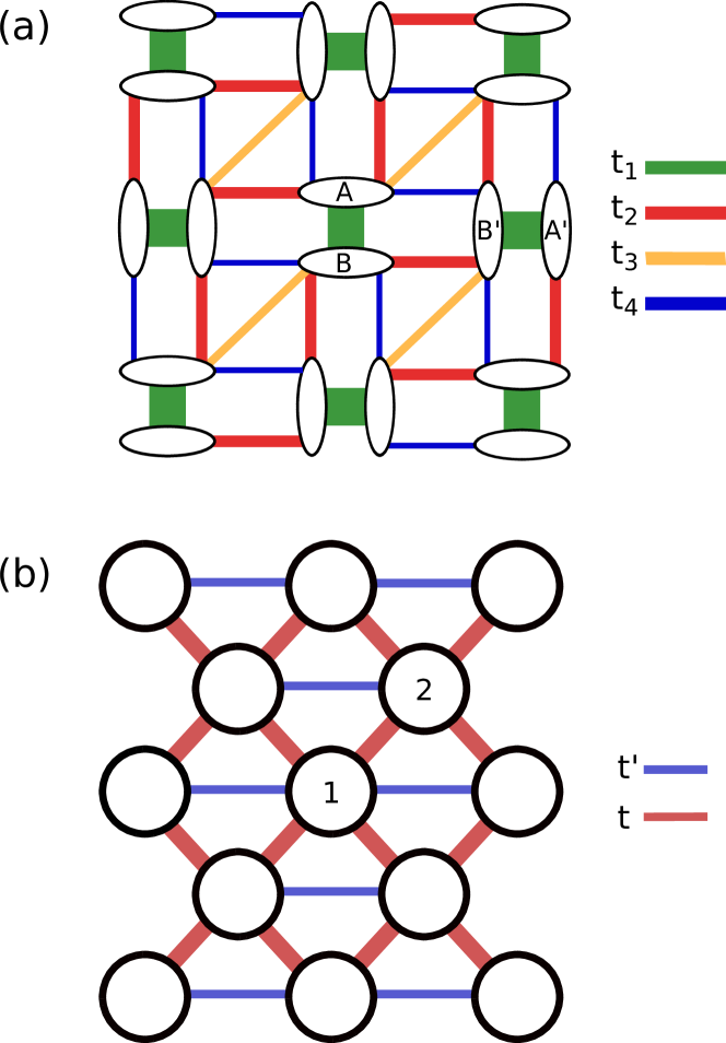
Figure 1: (a) Lattice structure within the molecule model of the $\kappa$-(ET)${}_{2}^{+}$ layer. ET molecules are single lattice sites (ellipsoids in figure). The amplitude of the four dominant hopping integrals ($t_{1}$,$t_{2}$,$t_{3}$,$t_{4}$) are shown by the thickness of the line. (b) In the dimer model one has to integrate out $t_{1}$ and average between $t_{2}$ and $t_{4}$ that results in the dominant hopping integral $t$ while $t^{\prime}$ is connected to the former $t_{3}$ by dividing contributions from the two separate ET molecules that are counted now as one.

The parameters of the dimer model

$$H_{\text{kin}} =\sum_{\langle ij\rangle,\alpha,\sigma}t\left(c^{\dagger}_{\alpha,\sigma}(\vec{r}_{i})c_{\alpha,\sigma}(\vec{r}_{j})+h.c.\right)$$

$$+\sum_{[ij],\alpha,\beta,\alpha\neq\beta}t^{\prime}\left(c^{\dagger}_{\alpha,\sigma}(\vec{r}_{i})c_{\beta,\sigma}(\vec{r}_{j})+h.c.\right)$$

$$-\mu\sum_{i,\alpha,\sigma}c^{\dagger}_{\alpha,\sigma}(\vec{r}_{i})c_{\alpha,\sigma}(\vec{r}_{i})$$ (2)

can be derived using the geometrical relations

$$t =(|t_{2}|+|t_{4}|)/2$$ (3a)

$$t^{\prime} =|t_{3}|/2.$$ (3b)

The tight binding dispersions can be easily determined analytically through the four matrix elements between the two dimer states $|\alpha=0\rangle$ and $|\alpha=1\rangle$ in the dimer model,

$$\langle 0|H_{\text{kin}}|0\rangle(\vec{k})= \langle 1|H_{\text{kin}}|1\rangle(\vec{k})=2t^{\prime}\text{cos}(k_{x}a)-\mu$$ (4a)

$$\langle 0|H_{\text{kin}}|1\rangle(\vec{k})= t\left(e^{ik_{x}a/2+ik_{y}b/2}+e^{-ik_{x}a/2+ik_{y}b/2}+\right.$$

$$\left.+e^{ik_{x}a/2-ik_{y}b/2}+e^{-ik_{x}a/2-ik_{y}b/2}\right)$$

$$= \langle 1|H_{\text{kin}}|0\rangle^{\ast}(\vec{k})$$ (4b)

and six distinct contributions between the four molecule states for the molecule model

$$\langle 0|H_{\text{kin}}|1\rangle(\vec{k}) =t_{1}+t_{3}\,e^{ik_{x}a}$$ (5a)

$$\langle 0|H_{\text{kin}}|2\rangle(\vec{k}) =t_{4}\left(1+e^{-ik_{y}b}\right)$$ (5b)

$$\langle 0|H_{\text{kin}}|3\rangle(\vec{k}) =t_{2}\left(1+e^{-ik_{x}a}\right)$$ (5c)

$$\langle 1|H_{\text{kin}}|2\rangle(\vec{k}) =t_{2}\,e^{-ik_{y}b}\left(1+e^{-ik_{x}a}\right)$$ (5d)

$$\langle 1|H_{\text{kin}}|3\rangle(\vec{k}) =t_{4}\,e^{-ik_{x}a}\left(1+e^{-ik_{y}b}\right)$$ (5e)

$$\langle 2|H_{\text{kin}}|3\rangle(\vec{k}) =t_{1}+t_{3}\,e^{-ik_{x}a}$$ (5f)

$$\langle\alpha|H_{\text{kin}}|\alpha\rangle(\vec{k}) =-\mu,$$ (5g)

where $a$ and $b$ are lattice constants of the two-dimensional ET plane and the remaining matrix elements are obtained from $H=H^{\dagger}$. Note that the chemical potential was determined numerically to ensure the correct filling in both models.

II.2 Two-Particle Self-Consistent calculations

Due to the similarity of the phase diagram of cuprates and $\kappa$-(ET)₂ materials we can assume a spin-fluctuation based mechanism for the superconductivity. We will use an extension of the Two-Particle Self-Consistent (TPSC) approach as introduced by Vilk and Tremblay Vilk and Tremblay (1997) to find an approximate solution for our multi-site dimer and molecule models with Hubbard on-site interaction,

$$\begin{array}[]{rl}H=&H_{\text{kin}}+H_{\text{int}}\\ =&H_{\text{kin}}+\frac{U}{2}\sum\limits_{i,\alpha,\sigma}n_{\alpha\sigma}(\vec{r}_{i})n_{\alpha\bar{\sigma}}(\vec{r}_{i}),\end{array}$$ (6)

where $U$ is the Hubbard on-site interaction and $n_{i\alpha\sigma}$ is the number operator for electrons in unit cell $i$ at site $\alpha$ with spin $\sigma$. Note that the on-site $U$ term in the dimer model corresponds to the Coulomb interaction in the dimer where one can approximate Powell and McKenzie (2005, 2006) $U_{\text{dim}}\approx 2t_{1}$, while the on-site $U$ in the molecule model corresponds to the Coulomb interaction in the molecule $U_{\text{mol}}$. In the present work we do not include inter-site Coulomb contributions Kaneko et al. (2017). Please note that the inclusion of intermolecular Coulomb repulsion allows for the possibility of describing charge density wave phases in proximity to superconductivity Sekine et al. (2013); Watanabe et al. (2017). However, the observed solutions are very similar and we can only speculate that this may be due to a robustness of the instabilities that yield the resulting gap symmetries against further-neighbor interactions.

So far, TPSC has been successfully applied, f.i., to investigate pseudogap physics Tremblay (2011) and the dome-like shape of the superconducting critical temperature Ogura and Kuroki (2015); Kyung et al. (2003) for the Hubbard model on a square lattice. TPSC is a conserving and self-consistent approximation, in which higher order contributions to the four-point vertices are reduced to their averages. As a consequence, the resulting equations yield a weak- to intermediate-coupling approach for the solution of the Hubbard model.

We define the non-interacting multi-site Green’s function

$$\begin{array}[]{rl}G^{0}_{\mu\nu}(\vec{k},i\omega_{n})=\left[i\omega_{n}\mathbb{I}-H_{\text{kin}}(\vec{k})\right]^{-1}_{\mu\nu},\end{array}$$ (7)

where $\mu,\nu$ are site indices, $\vec{k}$ is a two-dimensional reciprocal lattice vector, and $\omega_{n}=(2n+1)\pi~{}T$ are fermionic Matsubara frequencies at temperature $T$. Moreover, we calculate the non-interacting susceptibility $\chi^{0}$

$$\begin{array}[]{rl}\chi^{0}_{\lambda\mu\nu\xi}(\vec{q},iq_{m})=-\frac{1}{N_{\vec{k}}}\sum\limits_{\vec{k},b,c}&a^{\nu}_{b}(\vec{k})a^{\lambda\ast}_{b}(\vec{k})a^{\mu}_{c}(\vec{k}+\vec{q})a^{\xi\ast}_{c}(\vec{k}+\vec{q})\\ &\displaystyle\times\frac{f(\epsilon_{b}(\vec{k}))-f(\epsilon_{c}(\vec{k}+\vec{q}))}{iq_{m}+\epsilon_{b}(\vec{k})-\epsilon_{c}(\vec{k}+\vec{q})}\end{array}$$ (8)

where matrix elements $a_{\mu,a}$ as well as energy eigenvalues $\epsilon_{a}(\vec{k})$ are obtained by diagonalization of the tight-binding Hamiltonian $H_{\text{kin}}$. In order to facilitate the assignment of indices, we will follow the convention that greek letters denote site indices and latin letters denote band indices. Moreover, the susceptibility depends on the difference of the thermal occupation probability $f(x)=\frac{1}{1+e^{x/(k_{B}T)}}$, which follows from Fermi-Dirac statistics, and bosonic Matsubara frequencies $iq_{m}=2m\pi~{}T$. For $iq_{m}=0$, the denominator becomes divergent for equal band energies, which we treat by means of the rule of l’Hospital. Due to the fact that the considered Hamiltonians bear no non-local interactions, for susceptibilities of the form $\chi_{\mu\mu\nu\nu}$ (see below) we can reduce the tensor product of vector spaces from $\mathbb{C}^{N}\otimes\mathbb{C}^{N}\otimes\mathbb{C}^{N}\otimes\mathbb{C}^{N}$ to $\mathbb{C}^{N}\otimes\mathbb{C}^{N}$.

Spin and charge fluctuations within TPSC are treated by spin and charge susceptibilities ($\chi^{\text{sp}}$ and $\chi^{\text{ch}}$ respectively) from linear response theory.

$$\begin{array}[]{rl}\chi^{\text{sp}}(\vec{q},iq_{m})&=[\mathbb{I}-U^{\text{sp}}\chi^{0}(\vec{q},iq_{m})]^{-1}2\chi^{0}(\vec{q},iq_{m})\\ \chi^{\text{ch}}(\vec{q},iq_{m})&=[\mathbb{I}+U^{\text{ch}}\chi^{0}(\vec{q},iq_{m})]^{-1}2\chi^{0}(\vec{q},iq_{m}).\end{array}$$ (9)

The renormalized irreducible vertices in the spin channel $U^{\text{sp}}$ and in the charge channel $U^{\text{ch}}$ are determined by local spin and charge sum rules

$$\begin{array}[]{rl}\frac{T}{N_{\vec{q}}}\sum\limits_{\vec{q},iq_{m}}\chi^{\text{sp}}_{\mu\mu}(\vec{q},iq_{m})&=n_{\mu}-2\langle n_{\mu\uparrow}n_{\mu\downarrow}\rangle\\ \frac{T}{N_{\vec{q}}}\sum\limits_{\vec{q},iq_{m}}\chi^{\text{ch}}_{\mu\mu}(\vec{q},iq_{m})&=n_{\mu}+2\langle n_{\mu\uparrow}n_{\mu\downarrow}\rangle-n^{2}_{\mu},\end{array}$$ (10)

where the spin vertex $U^{\text{sp}}$ is calculated from an ansatz equation that is motivated by the Kanamori-Brueckner screening Vilk and Tremblay (1997)

$$\begin{array}[]{rl}U^{\text{sp}}_{\mu\nu}=\frac{\langle n_{\mu\uparrow}n_{\mu\downarrow}\rangle}{\langle n_{\mu\uparrow}\rangle\langle n_{\mu\downarrow}\rangle}U\delta_{\mu,\nu}\end{array}$$ (11)

and the diagonal elements of the charge vertex $U^{\text{ch}}_{\mu\mu}$ are directly calculated from the local charge sum rule while off-diagonal elements are zero. Correlation effects within the Green’s function $G$ are taken into account using a single-shot self-energy $\Sigma$ and incorporated by the Dyson equation

$$\Sigma_{\mu\nu}(\vec{k},i\omega_{n}) =Un_{\mu,-\sigma}\delta_{\mu,\nu}+\frac{UT}{8N_{\vec{q}}}\sum\limits_{\vec{q},iq_{m}}\left[3U^{\text{sp}}_{\mu\mu}\chi^{\text{sp}}_{\mu\nu}(\vec{q},iq_{m})+U^{\text{ch}}_{\mu\mu}\chi^{\text{ch}}_{\mu\nu}(\vec{q},iq_{m})\right]G^{0}_{\mu\nu}(\vec{k}-\vec{q},i\omega_{n-m})$$ (12)

$$G_{\mu\nu}(\vec{k},i\omega_{n}) =\left[{G^{0}}^{-1}_{\mu\nu}(\vec{k},i\omega_{n})-\Sigma_{\mu\nu}(\vec{k},i\omega_{n})\right]^{-1}.$$ (13)

In this framework, we employ Migdal-Eliashberg theory to calculate the superconducting gap $\Delta_{\mu\nu}(\vec{k},i\omega_{n})$. We restrict our calculations to singlet and even-frequency and -orbital solutions, i.e.

$$\Delta_{\mu\nu}(\vec{k},i\omega_{n})=\Delta_{\mu\nu}(-\vec{k},i\omega_{n})=\Delta_{\mu\nu}(\vec{k},-i\omega_{n}).$$ (14)

The linearized Eliashberg equation takes the form

$$\lambda\Delta_{\mu\nu}(\vec{k},i\omega_{n}) =\frac{T}{N_{\vec{k}^{\prime}}}\sum_{\vec{k}^{\prime},i\omega_{n^{\prime}}}V_{\mu\nu}(\vec{k}-\vec{k}^{\prime},iq_{n-n^{\prime}})\sum_{\alpha,\beta}G_{\mu\alpha}(\vec{k}^{\prime},i\omega_{n^{\prime}})\Delta_{\alpha\beta}(\vec{k}^{\prime},i\omega_{n^{\prime}})G^{\ast}_{\nu\beta}(\vec{k}^{\prime},i\omega_{n^{\prime}})$$ (15)

where the temperature at which the largest positive eigenvalue $\lambda$ becomes unity indicates the onset of superconductivity. The singlet pairing potential is calculated within the Random Phase Approximation (RPA Bickers et al. (1989); Scalapino et al. (1986)) and given by

$$V(\vec{q},iq_{m})=-\frac{3}{4}U^{\text{sp}}\chi^{\text{sp}}(\vec{q},iq_{m})U+\frac{1}{4}U^{\text{ch}}\chi^{\text{ch}}(\vec{q},iq_{m})U-\frac{1}{2}U.$$

We enforce singlet solutions by symmetrization of the gap $(G\Delta G)_{\mu\nu}^{s}(\vec{k},i\omega_{n})=\frac{1}{2}\left[(G\Delta G)_{\mu\nu}(\vec{k},i\omega_{n})+(G\Delta G)_{\nu\mu}(-\vec{k},-i\omega_{n})\right]$ entering on the right-hand-side of the linearized Eliashberg equation (Eq. 15). For the numerical evaluation of the non-interacting susceptibility we employed adaptive cubature based on a three-point formula for triangles with an integration tolerance of $10^{-6}$. The interacting susceptibilities are strongly peaked when approaching the critical temperature. Therefore they were calculated on a $200\times 200$ k grid for the molecule model and $300\times 300$ k grid for the dimer model, while all other quantitities were well-converged on $70\times 70$ grids. For the evaluation of Eqs. 12 and 15, we additionally employed fast Fourier transforms and the circular convolution theorem for a highly efficient implementation. The summation over Matsubara frequencies was performed for $N_{\text{Mats}}=40\cdot(0.025/T)$ points, whereas high-frequency corrections up to the order of $\frac{1}{\omega^{2}}$ were included by extrapolation.

III Results and Discussion

III.1 Half-filled dimer model

Although the insufficiency of the dimer model for capturing the physics of the $\kappa$-(ET)₂X systems has been discussed Guterding et al. (2016b); Watanabe et al. (2017), we will first use this well-explored model as a benchmark for our TPSC calculations.

In the context of the high-Tc cuprate superconductors it is already well known that the half-filled single-band Hubbard model on the square lattice stabilizes d${}_{x^{2}-y^{2}}$ pairing solutions. Introducing anisotropic diagonal couplings $t^{\prime}$ one expects superconductivity to become unstable for high values of the frustration $t^{\prime}/t$, while the d-wave solution will be retained for intermediate frustration strengths, as it is the case for the half-filled single-band triangular lattice model for $\kappa$-(ET)₂X. In order to compare the results of this section to the molecule model considered in the following section, we have to transform this solution to the physical Brillouin zone (BZ) of the $\kappa$-(ET)₂X (corresponding to two dimers per crystallographic unit cell), which is half as large as of the single-band model. Folding the BZ corners and rotating by 45° Guterding et al. (2016b), we expect a d_xy solution with gap maxima at ($\pm\pi,\pm\pi$). Additionally, the $2\pi$ periodicity of the gap function enforces node-lines along the BZ boundaries ($k_{x},\pi$) and ($\pi,k_{y}$). Note that there is a sign change between the two bands at the Fermi surface (see Fig. 2), which previously has been attributed to strong inter-band coupling Schmalian (1998).

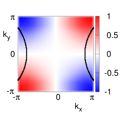
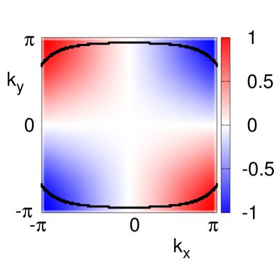
Figure 2: Superconducting gap $\Delta(\vec{k},i\omega_{0})$ of the dimer model in the first physical Brillouin zone (see main text). The dominant d_xy character shows nodes along the boundaries, since it has to be 2$\pi$ periodic, and a sign change between (a) the first band and (b) the second band that has been previously assigned to strong inter-band coupling Schmalian (1998).

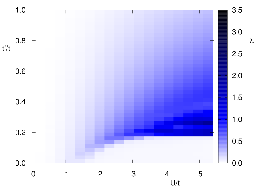
Figure 3: Largest positive eigenvalue of the linearized Eliashberg equation at T=0.003 eV within the dimer model. Moderate on-site interactions are crucial to obtain superconductivity, while too strong correlations ($U_{\text{dim}}/t\gtrsim 1.5$) result in the opening of a pseudogap and Mott insulator physics. Strong afm insulating tendencies can be reduced by next nearest neighbor hoppings and the implicit geometric frustration. A combination of both ($t^{\prime}/t\approx 0.25$ and $U_{\text{dim}}/t>3.4$) is most favorable for superconductivity.

material	$t^{\prime}/t$	$t_{4}/t_{2}$	$U_{\text{dim}}$ [eV]	$T^{\text{TPSC}}_{c}$ [K]	$T_{c}$ Hiramatsu et al. (2015); Kato et al. (1987); Mori et al. (1990); Kini et al. (1990) [K]
$\kappa$-(ET)2Ag(CF3)4(TCE)	0.449	0.362	0.336	32.5	2.6
$\kappa$-(ET)2I3	0.346	0.266	0.36	44.1	3.6
$\kappa$-(ET)2Ag(CN)2I$\cdot$H2O	0.473	0.305	0.37	31.3	5.0
$\kappa$-$\alpha^{\prime}_{1}$-(ET)2Ag(CF3)4(TCE)	0.495	0.362	0.332	27.1	9.5
$\kappa$-(ET)2Cu(NCS)2	0.69	0.171	0.38	15	10.4
$\kappa$-$\alpha^{\prime}_{2}$-(ET)2Ag(CF3)4(TCE)	0.495	0.369	0.33	26.2	11.1
$\kappa$-(ET)2Cu[N(CN)2](CN)	0.669	0.172	0.35	13.9	11.2
$\kappa$-(ET)2Cu[N(CN)2]Br	0.455	0.379	0.354	32.5	11.6

Table 1: Comparison of the calculated and experimental critical temperatures $T_{c}$ for several organic charge transfer salts. The calculations within the dimer model do not reproduce the general trend of the experimental results but can be understood by means of geometric frustration (see Fig. 4).

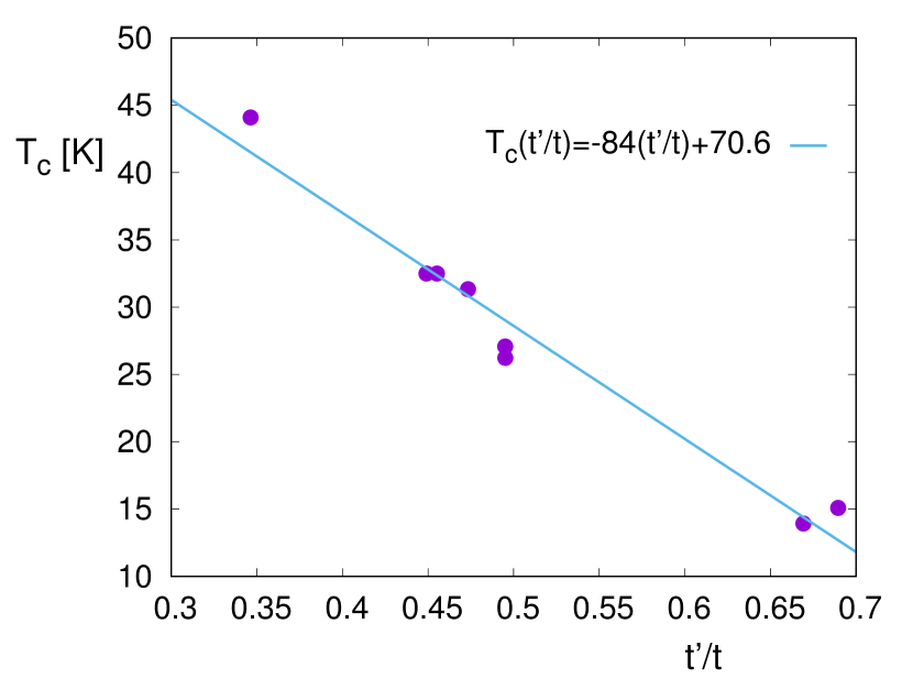
Figure 4: Critical temperature T_c calculated within the combined TPSC + Eliashberg approach as a function of $t^{\prime}/t$ for the eight $\kappa$-(ET)₂X materials listed in Table 1. T_c drops monotonically with increasing $t^{\prime}/t$ since the geometric frustration suppresses an afm state und reduces therefore spin fluctuations that are key ingredients for large T_c. As a guide to the eye we show the linear fit to the data points.

In order to explore the role of the diagonal hopping $t^{\prime}$ we have calculated the largest positive eigenvalue of the linearized Eliashberg equation (Eq. 15) at $T=0.003$ eV$\approx 35$ K in dependence of the hopping ratio $t^{\prime}/t$ and the relative on-site repulsion $U_{\text{dim}}/t$ (Fig. 3), where a large eigenvalue implies a close proximity to the superconducting state that is realized at $\lambda=1$. We find that several effects compete: at large $t^{\prime}/t$ ratios the antiferromagnetic (afm) fluctuations that drive superconductivity, are strongly suppressed, while for large correlations a pseudogap opens, reducing the number of states close to the Fermi level and therefore the total energy gained by the formation of superconducting pairs. Therefore, both effects are needed to enhance spin fluctuations but they should be kept moderate enough to prevent magnetic ordering.

Finally, we calculate critical temperatures for eight representatives of the $\kappa$-(ET)₂X family for $U_{\text{dim}}\approx 2t_{1}$ (see Tab. 1). We observe no obvious relation to the measured critical temperatures. However, plotting the calculated critical temperatures against the corresponding frustration values (Fig. 4), we find a monotonous decrease with increasing geometric frustration, i.e., the diagonal hopping suppresses the afm spin fluctuations that drive the superconductivity. As the measured critical temperatures do not follow this simple trend, it is obvious that we have to go beyond the dimer model in order to understand the superconductivity in the $\kappa$-(ET)₂X family.

III.2 3/4-filled molecule model

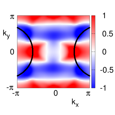
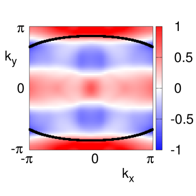
Figure 5: s_±+d${}_{x^{2}-y^{2}}$ superconducting gap $\Delta(\vec{k},i\omega_{0})$ as obtained in the four band molecule model at low temperatures. This kind of symmetry was already observed in Ref. Guterding et al., 2016b in the context of RPA calculations.

Figure 6: Largest positive eigenvalue $\lambda$ of the linearized Eliashberg equation for $U_{\text{mol}}=0.65$ eV. We see only small differences between the values for each material which can be understood from the similarity of the hopping parameters. The four band model based on the largest hopping elements is not sufficient to reproduce the trends of $T_{c}$.

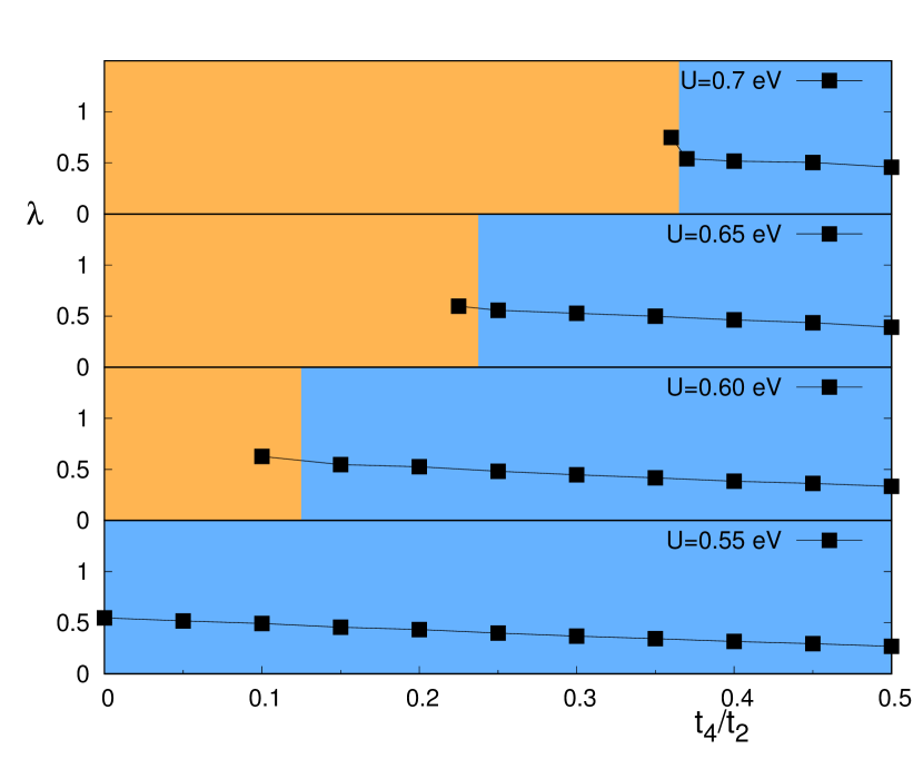
Figure 7: Largest positive eigenvalue $\lambda$ of the linearized Eliashberg equation for $U_{\text{mol}}=0.55,0.6,0.65\text{ and }0.7~{}eV$ ($t_{1},t_{2}$ and $t_{3}$ averaged from GGA results Guterding et al. (2016b)). We see an overall increase in $\lambda$ by going to larger values of $U_{\text{mol}}$ and an inset of extended $s+d_{x^{2}-y^{2}}$ gap symmetry (orange background) at small values of $t_{4}/t_{2}$ while $d_{xy}$ symmetry (blue background) is dominant otherwise.

We consider now the proposed four-parameter molecule model Guterding et al. (2016b) as the starting point of the present study (the comparison to the full ab initio derived tight-binding model is discussed in Appendix B).

In the molecule model, the center of each ET molecule constitutes a lattice site in the tight binding model yielding a three quarter filled four-band system (four molecules per unit cell). Compared to the dimer model two additional degrees of freedom are accessible: the strength of the intra-dimer hopping and the in-plane anisotropy. In a previous study Guterding et al. (2016b) it was demonstrated that already a small degree of in-plane anisotropy results in considerable symmetry changes of the gap function. For all realistic parameter sets the exotic eight-node gap function was found to be favorable, whereas several compounds were shown to lie close to a phase boundary to d_xy symmetry.

As the previous static RPA approach may only give qualitative results on the gap symmetry, in this study we apply the above introduced combination of the linearized Eliashberg equation, the RPA expression for the pairing vertex and the TPSC self-energy corrected Green’s functions and renormalized vertices.

Interestingly, the gap symmetries calculated with the more advanced TPSC approach differ from the RPA predictions. For moderate on-site molecule $U_{\text{mol}}$ values, only $\kappa$-(ET)₂Cu(NCS)₂ and $\kappa$-(ET)₂Cu[N(CN)₂](CN), with the highest in-plane anisotropies feature s_±+d${}_{x^{2}-y^{2}}$ symmetry (see Fig. 5), while the other compounds exhibit a simple d_xy symmetry as in the dimer model. Only for larger values of $U_{\text{mol}}$ s_±+d${}_{x^{2}-y^{2}}$ is stabilized in a large region in parameter space including all superconducting materials studied with RPA if $U_{\text{mol}}\gtrsim 0.7eV$ (see Fig. 7). This result and the experimental evidence of s_±+d${}_{x^{2}-y^{2}}$ gap symmetry in $\kappa$-(ET)₂Cu[N(CN)₂]Br Guterding et al. (2016a) indicate the importance of correlations in these materials not only for the enhancement of spin-fluctuations but also for the symmetry of the gap function. Although the TPSC approach - in general - also allows us to determine the critical temperatures for superconductivity, we find that correlation effects give rise to strong antiferromagnetic fluctuations (as indicated by diverging spin susceptibilities) in TPSC, that do not allow us to obtain meaningful results in the $\lambda\approx 1$ regime for the molecule model. Therefore, we can only estimate trends for the critical temperatures from the magnitude of the eigenvalue of the Eliashberg equation at higher temperatures above the superconducting transition, as displayed in Fig. 6, where we assumed $U_{\text{mol}}=0.65~{}$eV. We find that although the two materials with the $s_{\pm}+d_{x^{2}-y^{2}}$ solution show the strongest deviations in the hopping parameters, they are located on the same branch as most of the other materials. Instead, $\kappa$-(ET)₂Ag(CN)₂I$\cdot$H₂O and $\kappa$-(ET)₂Cu[N(CN)₂]Br, exhibit especially high eigenvalues in the considered temperature range that do not coincide with experimental observations. Nevertheless, it is interesting to note that also the $s_{\pm}+d_{x^{2}-y^{2}}$ compounds prefer a $d_{xy}$ solution at high temperatures above the superconducting transition (see appendix A). Only below $\sim 20$ K the eight-node solution is stabilized, although the susceptibilities already reveal the tendency towards the $s_{\pm}+d_{x^{2}-y^{2}}$ solution at higher temperatures (see Fig. 8 in the appendix A). While the spin susceptibilities of the materials displaying $d_{xy}$ symmetry in the considered parameter range peak at reciprocal vectors $q\sim(0.6\pi,0.37\pi)$, the peaks are significantly shifted to higher $q_{x}$ values for the two compounds with high in-plane anisotropies, $q\sim(0.76\pi,0.41\pi)$. Moreover, as mentioned above, in the TPSC calculations the magnitude of the on-site Hubbard repulsion strongly influences the gap symmetry. At low values of the Hubbard interaction it is not possible to access the $s_{\pm}+d_{x^{2}-y^{2}}$ region for any strength of the in-plane anisotropy, while slightly larger values shift the transition line towards $t_{4}/t_{2}$ values of up to $0.365$ for $U_{\text{mol}}=0.7eV$ (see Fig. 7).

IV Summary and Outlook

To summarize, we have applied a combination of TPSC and the Eliashberg framework for superconductivity in order to derive the gap symmetries and trends for the critical temperatures in the dimer and molecule models for several superconducting $\kappa$-(ET)₂X materials. Within the dimer model we find that the critical temperatures only reflect the frustration of the system but do not reproduce the experimental trends. Our calculations for the molecule model confirm previous findings that the additional degrees of freedom, i.e. the intra-dimer hopping and the in-plane anisotropy, are decisive for the gap symmetry and can result in $s_{\pm}+d_{x^{2}-y^{2}}$ solutions. However, we find that the $s_{\pm}+d_{x^{2}-y^{2}}$ gap is further stabilized by increasing correlations and may therefore be realized within the range of realistic model parameters. These three tuning parameters are known to be very sensitive to pressure or strain as well as to endgroup disorder. Switching between the different gap symmetries may therefore be easily realizable and should be observable in f.i. state-of-the-art scanning tunneling spectroscopy measurements.

Appendix A Temperature dependence of gap symmetry

Our combined TPSC and Eliashberg framework allows us to track the gap symmetry and the corresponding eigenvalue at temperatures above the superconducting transition. Interestingly, we find that at high temperatures, $T\gg T_{c}$, all materials yield a $d_{xy}$ symmetry. Only at temperatures close to the superconducting transition, the materials with high in-plane anisotropy and/or large correlations undergo a transition to the extended s+d${}_{x^{2}-y^{2}}$ symmetry accompanied by a change of the slope and a non-monotonous jump in the Eliashberg eigenvalue, as shown in Fig. 8 for the $\kappa$-(ET)₂Cu(NCS)₂ compound. This small drop in the eigenvalue can be interpreted in terms of a competition between the different order parameter symmetries, which destabilizes the superconducting state.

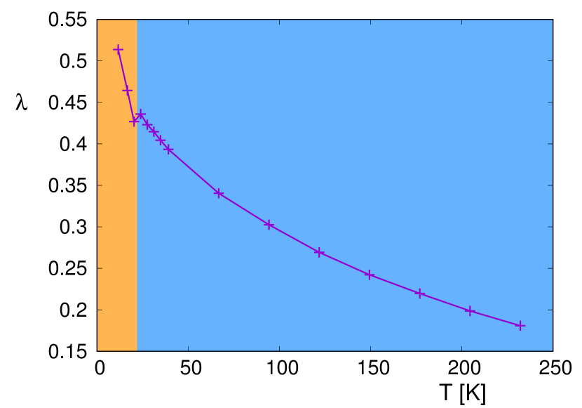
Figure 8: Largest eigenvalue $\lambda$ of the linearized Eliashberg equation for $\kappa$-(ET)₂Cu(NCS)₂ in the four-parameter model with $U_{mol}=0.65$ eV. A change in the gap symmetry (from d_xy to extended s+d${}_{x^{2}-y^{2}}$) becomes visible at T$\approx$22 K and is accompanied by a sudden drop in the eigenvalue that can be understood as a suppression of the superconducting state due to competing symmetries.

Appendix B Susceptibilities and gap symmetries

Based on the discussion of the temperature dependence of the gap symmetries, we think that all materials might exhibit $s_{\pm}+d_{x^{2}-y^{2}}$ gap symmetry at very low temperatures, at which we can not perform meaningful calculations due to diverging factors in the linearized Eliashberg equation. In order to resolve this issue, we further investigate the driving force of the superconducting transition, i.e., the spin susceptibilities. Indeed, we can find two clear distinctions between the high in-plane anisotropy materials and the other $\kappa$-ET materials (see Fig. 9): First, the broad shoulder connecting the one-dimensional parts of the Fermi surface is much less pronounced in the materials with high in-plane anisotropy. Second, the peak position is further shifted towards the Brillouin zone boundaries. While the strongest peaks in most of the materials are located at $(0.6\pi,0.37\pi)$, it is shifted to higher $k_{x}$, $k_{y}$ values, $(0.76\pi,0.41\pi)$, in $\kappa$-(ET)₂Cu(NCS)₂ and $\kappa$-(ET)₂Cu[N(CN)₂](CN).

Hence, a careful inspection of the spin susceptibilities even at high temperatures can give clues as to the necessary strength of the correlations to realize $s_{\pm}+d_{x^{2}-y^{2}}$ gap symmetries.

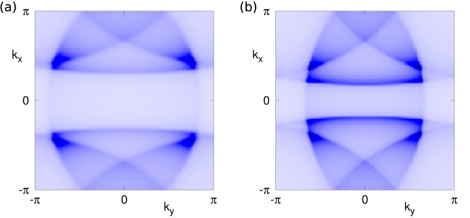
Figure 9: Static spin susceptibility $\sum_{\mu}\chi^{sp}_{\mu\mu}(\vec{q},0)$ for $s_{\pm}+d_{x^{2}-y^{2}}$ (a) and $d_{xy}$ (b) gap symmetries. The dominant spin fluctuations in the compounds with smaller in-plane anisotropy have wave vectors of about $(0.6\pi,0.37\pi)$, while the dominant vector is shifted towards large k values in the materials with high in-plane anisotropies, $Q\sim(0.76\pi,0.41\pi)$.

Appendix C Reduction to largest hopping elements

In order to rule out the possibility that inclusion of further hopping parameters crucially influences the gap symmetries or transition temperatures, we have performed test calculation, where we compare the four-parameter calculations with the results of calculations, in which we take into account the full Hamiltonian as obtained by the Wannier projection method in DFT. In Fig. 10 we show the temperature evolution of the largest Eliashberg eigenvalue for the two models for one representative of the $\kappa$-ET family. While we always obtain the same gap symmetry independent of the considered model, the eigenvalue is considerably enhanced due to the additional hoppings. Hence, we want to stress that accurate calculations of critical temperatures do not only have to carefully choose the strength of the Hubbard repulsion but also have to go beyond the four-parameter model.

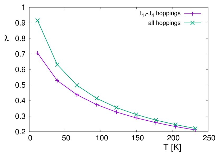
Figure 10: Temperature evolution of the largest Eliashberg eigenvalue $\lambda$ for the four-parameter (violet line) and full ab initio derived kinetic Hamiltonian (green line) for $\kappa$-(ET)₂Cu[N(CN)₂]Br with $U_{mol}=0.65$ eV. While the gap symmetry remains unchanged, the inclusion of long-range hoppings stabilizes the superconducting state.

References

- Toyota et al. (2007) N. Toyota, M. Lang, and J. Müller, Low-Dimensional Molecular Metals (Springer-Verlag Berlin Heidelberg, 2007).
- Powell and McKenzie (2005) B. J. Powell and R. H. McKenzie, Phys. Rev. Lett. 94, 047004 (2005).
- Shimizu et al. (2003) Y. Shimizu, K. Miyagawa, K. Kanoda, M. Maesato, and G. Saito, Phys. Rev. Lett. 91, 107001 (2003).
- Dumm et al. (2009) M. Dumm, D. Faltermeier, N. Drichko, M. Dressel, C. Mézière, and P. Batail, Phys. Rev. B 79, 195106 (2009).
- Kawaga et al. (2005) F. Kawaga, K. Miyagawa, and K. Kanoda, Nature 436, 534 (2005).
- Hartmann et al. (2014) B. Hartmann, J. Müller, and T. Sasaki, Phys. Rev. B 90, 195150 (2014).
- Guterding et al. (2015) D. Guterding, R. Valentí, and H. O. Jeschke, Phys. Rev. B 92, 081109(R) (2015).
- Hiramatsu et al. (2015) T. Hiramatsu, Y. Yoshida, G. Saito, A. Otsuka, H. Yamochi, M. Maesato, Y. Shimizu, H. Ito, and H. Kishida, J. Mater. Chem. C 3, 1378 (2015).
- Kato et al. (1987) R. Kato, H. Kobayashi, A. Kobayashi, S. Moriyama, Y. Nishio, K. Kajita, and W. Sasaki, Chem. Lett. 16, 507 (1987).
- Mori et al. (1990) H. Mori, I. Hirabayashi, S. Tanaka, T. Mori, and H. Inokuchi, Solid State Commun. 76, 35 (1990).
- Kini et al. (1990) A. M. Kini, U. Geiser, H. H. Wang, K. D. Carlson, J. M. Williams, W. K. Kwok, K. G. Vandervoort, J. E. Thompson, D. L. Stupka, D. Jung, and M.-H. Whangbo, Inorg. Chem. 29, 2555 (1990).
- Elsinger et al. (2000) H. Elsinger, J. Wosnitza, S. Wanka, J. Hagel, D. Schweitzer, and W. Strunz, Phys. Rev. Lett. 84, 6098 (2000).
- Müller et al. (2002) J. Müller, M. Lang, R. Helfrich, F. Steglich, and T. Sasaki, Phys. Rev. B 65, 140509(R) (2002).
- Wosnitza et al. (2003) J. Wosnitza, S. Wanka, J. Hagel, M. Reibelt, D. Schweitzer, and J. A. Schlueter, Synth. Met. 133, 201 (2003).
- Taylor et al. (2007) O. J. Taylor, A. Carrington, and J. A. Schlueter, Phys. Rev. Lett. 99, 057001 (2007).
- Taylor et al. (2008) O. J. Taylor, A. Carrington, and J. A. Schlueter, Phys. Rev. B 77, 060503(R) (2008).
- Malone et al. (2010) L. Malone, O. J. Taylor, J. A. Schlueter, and A. Carrington, Phys. Rev. B 82, 014522 (2010).
- Milbradt et al. (2013) S. Milbradt, A. A. Bardin, C. J. S. Truncik, W. A. Huttema, A. C. Jacko, P. L. Burn, S. C. Lo, B. J. Powell, and D. M. Broun, Phys. Rev. B 88, 064501 (2013).
- Izawa et al. (2001) K. Izawa, H. Yamaguchi, T. Sasaki, and Y. Matsuda, Phys. Rev. Lett. 88, 027002 (2001).
- Schrama et al. (1999) J. M. Schrama, E. Rzepniewski, R. S. Edwards, J. Singleton, A. Ardavan, M. Kurmoo, and P. Day, Phys. Rev. Lett. 83, 3041 (1999).
- Arai et al. (2001) T. Arai, K. Ichimura, K. Nomura, S. Takasaki, J. Yamada, S. Nakatsuji, and H. Anzai, Phys. Rev. B 63, 104518 (2001).
- Ichimura et al. (2008) K. Ichimura, M. Takami, and K. Nomura, J. Phys. Soc. Jpn. 77, 114707 (2008).
- Oka et al. (2015) Y. Oka, H. Nobukane, N. Matsunaga, K. Nomura, K. Katono, K. Ichimura, and A. Kawamoto, J. Phys. Soc. Jpn. 84, 064713 (2015).
- Guterding et al. (2016a) D. Guterding, S. Diehl, M. Altmeyer, T. Methfessel, U. Tutsch, H. Schubert, M. Lang, J. Müller, M. Huth, H. O. Jeschke, R. Valentí, M. Jourdan, and H.-J. Elmers, Phys. Rev. Lett. 116, 237001 (2016a).
- Kühlmorgen et al. (2017) S. Kühlmorgen, R. Schönemann, E. L. Green, J. Müller, and J. Wosnitza, Journal of Physics: Condensed Matter 29, 405604 (2017).
- McKenzie (1997) R. H. McKenzie, Science 278, 820 (1997).
- Zhou et al. (2017) Y. Zhou, K. Kanoda, and T.-K. Ng, Rev. Mod. Phys. 89 (2017).
- Guterding et al. (2016b) D. Guterding, M. Altmeyer, H. O. Jeschke, and R. Valentí, Phys. Rev. B 94, 024515 (2016b).
- Vilk and Tremblay (1997) Y. M. Vilk and A.-M. S. Tremblay, J. Phys. I France 7, 1309 (1997).
- Kuroki et al. (2002) K. Kuroki, T. Kimura, R. Arita, Y. Tanaka, and Y. Matsuda, Phys. Rev. B 65, 100516(R) (2002).
- Schmalian (1998) J. Schmalian, Phys. Rev. Lett. 81, 4232 (1998).
- Powell and McKenzie (2006) B. J. Powell and R. H. McKenzie, Journal of Physics: Condensed Matter 18, R827 (2006).
- Kaneko et al. (2017) R. Kaneko, L. F. Tocchio, R. Valentí, and F. Becca, New J. Phys. 19, 103033 (2017).
- Sekine et al. (2013) A. Sekine, J. Nasu, and S. Ishihara, Phys. Rev. B 87, 085133 (2013).
- Tremblay (2011) A.-M. S. Tremblay, Two-Particle-Self-Consistent Approach for the Hubbard Model, edited by A. Avella and F. Mancini, 409-453 (Springer Berlin Heidelberg, 2011).
- Ogura and Kuroki (2015) D. Ogura and K. Kuroki, Phys. Rev. B 92, 144511 (2015).
- Kyung et al. (2003) B. Kyung, J.-S. Landry, and A. M. S. Tremblay, Phys. Rev. B 68, 174502 (2003).
- Bickers et al. (1989) N. E. Bickers, D. J. Scalapino, and S. R. White, Phys. Rev. Lett. 62, 961 (1989).
- Scalapino et al. (1986) D. J. Scalapino, E. Loh, and J. E. Hirsch, Phys. Rev. B 34, 8190 (1986).
- Watanabe et al. (2017) H. Watanabe, H. Seo, and S. Yunoki, J. Phys. Soc. Jpn. 86, 033703 (2017).
- Note (1) Although it is possible to obtain below K, those solutions are not reliable since the corresponding susceptibilities are strongly peaked and the numerical integrations yield increasingly large errors.
- Note (2) For higher values it was not possible to perform calculations down to temperatures since the spin susceptibilities of some compound start to diverge and hamper numerical integrations. However our calculations (Fig. 7) show that the parameter region for extended gap symmetry increases with larger correlation strenghts.