Upper large deviations bound for singular-hyperbolic attracting sets

Abstract.

We obtain a exponential large deviation upper bound for continuous observables on suspension semiflows over a non-uniformly expanding base transformation with non-flat singularities and/or discontinuities, where the roof function defining the suspension behaves like the logarithm of the distance to the singular/discontinuous set of the base map. To obtain this upper bound, we show that the base transformation exhibits exponential slow recurrence to the singular set.

The results are applied to semiflows modeling singular-hyperbolic attracting sets of $C^{2}$ vector fields. As corollary of the methods we obtain results on the existence of physical measures and their statistical properties for classes of piecewise $C^{1+}$ expanding maps of the interval with singularities and discontinuities. We are also able to obtain exponentially fast escape rates from subsets without full measure.

1. Introduction

Arguably one of the most important concepts in Dynamical Systems theory is the notion of physical (or $SRB$) measure. We say that an invariant probability measure $\mu$ for a flow $X^{t}$ is physical if the set

$$B(\mu)=\left\{z\in M:\lim_{t\to\infty}\frac{1}{t}\int_{0}^{t}\psi(X^{s}(z))\,ds=\int\psi\,d\mu,\forall\psi\in C^{0}(M,{\mathbb{R}})\right\}$$

has non-zero volume, with respect to any volume form on the ambient compact manifold $M$. The set $B(\mu)$ is by definition the basin of $\mu$. It is assumed that time averages of these orbits be observable if the flow models a physical phenomenon.

On the existence of physical/SRB measures for uniformly hyperbolic diffeomorphisms and flows we mention the works of Sinai, Ruelle and Bowen [26, 27, 59, 60, 66]. More recently, Alves, Bonatti and Viana [3] obtained the existence of physical measures for partial hyperbolic diffeomorphism and non-uniformly expanding transformations. Many developments along these lines for non uniformly hyperbolic systems have been obtained; see e.g. [56, 29, 23, 24, 16]. Closer to our setting, Araujo, Pacifico, Pujals and Viana [18] obtained physical measures for singular-hyperbolic attractors.

It is natural to study statistical properties of physical measures, such as the speed of convergence of the time averages to the space average, among many other properties which have been intensely studied recently; see e.g. [40, 70, 71, 25, 2, 6, 28, 48, 47, 32, 37, 44, 14, 11]. The main motivation behind all these results is that for chaotic systems the family $\left\{\psi\circ X^{t}\right\}_{t>0}$ asymptotically behaves like an i.i.d. family of random variables.

One of the ways to quantify this is the volume of the subset of points whose time averages $\frac{1}{T}S_{T}\psi$ are away from the space average $\mu(\psi)$ by a given amount. More precisely, fixing $\varepsilon>0$ as the error size, we consider the set

$$B_{T}=\left\{x\in M:\left|\frac{1}{T}\int_{0}^{T}\psi(X^{s}(x))ds-\int\psi\,d\mu\right|>\varepsilon\right\}$$

and search for conditions under which the volume of this set decays exponentially fast with $T$. That is, there are constants $C,\xi>0$ so that

$$Leb(B_{T})\leq Ce^{-\xi T},\mbox{ for all }T>0.$$

The decay rate is related to the Thermodynamical Formalism, first developed for hyperbolic diffeomorphisms by Bowen, Ruelle and Sinai; see e.g. [26, 27, 61, 62]. However, in our setting Lebesgue measure is not necessarily an invariant measure and so some tools from the Thermodynamical Formalism are unavailable.

This work extends and corrects the proof of the first author’s result [7] of upper large deviation estimate for the geometric Lorenz attractor to the singular-hyperbolic attracting setting, encompassing a much more general family of singular three-dimensional flows, not necessarily transitive, with several singularities and with higher dimensional stable direction.

This demanded, first, the construction of a global Poincaré map as in [18] through adapted cross-sections to the flow obtained without assuming transitivity; and, second, to deal with the possible existence of finitely many distinct ergodic physical measures whose convex linear combinations form the set ${\mathbb{E}}$ of equilibrium states with respect to the $\log$ of the central unstable Jacobian. This led us to adapt the strategy of reduction of set of deviations for the flow to a set of deviations for a one-dimensional map while still following the general path presented in [7].

This extension is done through a special choice of adapted cross-sections in the definition of the global Poincaré map which is shown to be always possible for singular-hyperbolic attracting sets of $C^{2}$ flows.

Finally, and technically more delicate, we extend and correct the proof of exponentially slow recurrence from [7, Section 6] for a piecewise expanding one-dimensional interval map with only singular discontinuities (with unbounded derivative) to allow both singularities (with unbounded derivative) and discontinuities (with bounded derivative) as boundary points of the monotonicity intervals of the one-dimensional map. In particular, this result allows us to obtain many statistical properties of a new class of piecewise expanding interval maps. This can be seen as an extension of [31] to Hölder-$C^{1}$ piecewise expanding maps with singularities and discontinuities, and also assuming strong interaction between them; see Section 1.3 for more comments.

1.1. The setting: singular-hyperbolicity

We need some preliminary definitions.

From now on $M$ is a compact boundaryless $d$-dimensional manifold; ${\mathfrak{X}}^{2}(M)$ is the set of $C^{2}$ vector fields on $M$, endowed with the $C^{2}$ topology; we fix some smooth Riemannian structure on $M$ and an induced normalized volume form $\operatorname{Leb}$ that we call Lebesgue measure; and we write also $\operatorname{dist}$ for the induced distance on $M$.

Given $X\in{{\mathfrak{X}}}^{2}(M)$, we write $X^{t}$, $t\in{\mathbb{R}}$ the flow induced by $X$ and, for $x\in M$ and $[a,b]\subset{\mathbb{R}}$ we set $X^{[a,b]}(x)=\{X^{t}(x),a\leq t\leq b\}$.

For a compact invariant set $\Lambda$ for $X\in{\mathfrak{X}}^{2}(M)$, we say that it is isolated if we can find an open neighborhood $U\supset\Lambda$ so that $\Lambda=\bigcap_{t\in{\mathbb{R}}}X^{t}(U)$. If $U$ above also satisfies $X^{t}(U)\subset U$ for $t>0$ then we say that $\Lambda$ is an attracting set and that $U$ is a trapping region for $\Lambda$. The topological basin of the attracting set $\Lambda$ is $W^{s}(\Lambda)=\{x\in M:\lim_{t\to+\infty}\operatorname{dist}\big{(}X^{t}(x),\Lambda\big{)}=0\}.$

The invariant set $\Lambda$ is transitive if it coincides with the $\omega$-limit set of a regular $X$-orbit: $\Lambda=\omega_{X}(p)$ where $p\in\Lambda$ and $X(p)\neq\vec{0}$. If $\sigma\in M$ and $X(\sigma)=0$, then $\sigma$ is called an equilibrium or singularity.

A point $p\in M$ is periodic if $p$ is regular and there exists $\tau>0$ so that $X^{\tau}(p)=p$; its orbit ${\mathcal{O}}_{X}(p)=X^{{\mathbb{R}}}(p)=X^{[0,\tau]}(p)$ is a periodic orbit. An invariant set of $X$ is non-trivial if it is neither a periodic orbit nor a singularity.

An attractor is a transitive attracting set. An attractor is proper if it is not the whole manifold.

Definition 1.1.

Let $\Lambda$ be a compact invariant set of $X\in{\mathfrak{X}}^{2}(M)$ , $c>0$, and $0<\lambda<1$. We say that $\Lambda$ has a $(c,\lambda)$-dominated splitting if the tangent bundle over $\Lambda$ can be written as a continuous $DX^{t}t$-invariant sum of sub-bundles $T_{\Lambda}M=E^{1}\oplus E^{2},$ (that is, $DX^{t}E^{i}_{x}=E^{i}_{X^{t}x},\forall t\in{\mathbb{R}},i=1,2$) such that for every $t>0$ and every $x\in\Lambda$, we have

$$\|DX^{t}\mid E^{1}_{x}\|\cdot\|DX^{-t}\mid E^{2}_{X^{t}(x)}\|<c\,\lambda^{t}.$$ (1.1)

We say that a $X$-invariant subset $\Lambda$ of $M$ is partially hyperbolic if it has a $(c,\lambda)$-dominated splitting, for some $c>0$ and $\lambda\in(0,1)$, such that the sub-bundle $E^{1}=E^{s}$ is uniformly contracting: for every $t>0$ and every $x\in\Lambda$ we have $\|DX^{t}\mid E^{s}_{x}\|<c\,\lambda^{t}.$

We assume that $E^{s}$ has codimension $2$ so that $E^{cu}$ is two-dimensional: $\dim E^{cu}_{\Lambda}=2$ and $\dim E^{s}_{\Lambda}=d_{s}=d-2$.

Let now $J_{t}^{cu}(x)$ be the center Jacobian of $DX^{t}$ for $x\in\Lambda$, that is, the absolute value of the determinant of the linear map $DX^{t}\mid E^{cu}_{x}:E^{cu}_{x}\to E^{cu}_{X^{t}(x)}.$ We say that the sub-bundle $E^{cu}_{\Lambda}$ of the partially hyperbolic invariant set $\Lambda$ is $(c,\lambda)$-volume expanding if $J_{t}^{cu}(x)\geq c\,e^{\lambda t}$ for every $x\in\Lambda$ and $t\geq 0$, for some given $c,\lambda>0.$

Definition 1.2.

Let $\Lambda$ be a compact invariant set of $X\in{\mathfrak{X}}^{2}(M)$ with singularities. We say that $\Lambda$ is a singular-hyperbolic set for $X$ if all the singularities of $\Lambda$ are hyperbolic and $\Lambda$ is partially hyperbolic with volume expanding central direction.

Singular-hyperbolicity is an extension of the notion of hyperbolic set, which we now recall.

Definition 1.3.

Let $\Lambda$ be a compact invariant set of $X\in{\mathfrak{X}}^{2}(M)$. We say that $\Lambda$ is a hyperbolic set for $X$ if it admits a continuous $DX^{t}$-invariant splitting $T_{\Lambda}M=E^{s}\oplus[X]\oplus E^{u}$ where $[X]={\mathbb{R}}\cdot X$ is the flow direction; $E^{s}$ is $(c,\lambda)$ contracting and $E^{u}$ is $(c,\lambda)$-contracting for the inverse flow, for some $(c,\lambda)\in{\mathbb{R}}^{+}\times(0,1)$.

In particular, every equilibrium point in a hyperbolic set must be isolated in the set. The following result shows that singular-hyperbolicity is a natural extension of notion of hyperbolicity for singular flows.

Theorem 1.4 (Hyperbolic Lemma).

A compact invariant singular-hyperbolic set without singularities is a hyperbolic set.

Proof.

See [52, Lemma 3] or [17, Proposition 6.2]. ∎

The most representative example of a singular-hyperbolic attractor is the Lorenz attractor; see e.g. [67, 68]. Singular-hyperbolic attracting sets form a class of attracting set sharing similar topological/geometrical features with the Lorenz attractor. For more on singular-hyperbolic attracting sets see e.g. [17].

1.1.1. Lorenz-like singularities

A Lorenz-like singularity is an equilibrium $\sigma$ of $X$ contained in a singular-hyperbolic set having index (dimension of the stable direction) equal to $d-1$. Since we are assuming that $\dim E^{c}=2$, this ensures the existence of the $DX(\sigma)$-invariant splitting $T_{\sigma}M=E^{s}_{\sigma}\oplus F^{s}_{\sigma}\oplus F^{u}_{\sigma}$ so that

• $E^{c}_{\sigma}=F^{s}\oplus F^{u}$ and $\dim F^{s}_{\sigma}=\dim F^{u}_{\sigma}=1$;

• $F^{u}_{\sigma}$ uniformly expands and $F^{s}_{\sigma}$ uniformly contracts: there exists $0<\widetilde{\lambda}<\lambda$ such that $\|DX^{t}\mid F^{u}_{\sigma}\|\geq C^{-1}\lambda^{-t}$ and $\|DX^{t}t\mid F^{s}_{\sigma}\|\leq C\widetilde{\lambda}^{t}$ for all $t\geq 0$.

Remark 1.5.

1. Partial hyperbolicity of $\Lambda$ implies that the direction $X(p)$ of the flow is contained in the center-unstable subbundle $E^{2}_{p}=E^{cu}_{p}$ at every point $p$ of $\Lambda$; see [8, Lemma 5.1].

2. The index of a singularity $\sigma$ in a singular-hyperbolic set $\Lambda$ equals either $\dim E^{s}_{\Lambda}$ or $1+\dim E^{s}_{\Lambda}$. That is, $\sigma$ is either a hyperbolic saddle with codimension $2$, or a Lorenz-like singularity.

3. If a singularity $\sigma$ in a singular-hyperbolic set $\Lambda$ is not Lorenz-like, then there is no orbit of $\Lambda$ that accumulates $\sigma$ in the positive time direction.

   Indeed, in this case ($\dim W^{s}_{\sigma}=\dim M-2$ and $\dim W^{u}_{\sigma}=2$), if $\sigma\in\omega(z)$ for $z\in\Lambda\setminus\{\sigma\}$, then there exists $p\in(W^{s}_{\sigma}\setminus\{\sigma\})\cap\omega(z)\subset\Lambda$ by the local behavior of trajectories near hyperbolic saddles. By the properties of the stable manifold $W^{s}_{\sigma}$, we have $X^{p}(p)\in W^{s}_{\sigma}\cap\Lambda,\forall t\geq 0$ and $T_{X^{t}(p)}W^{s}_{\sigma}\xrightarrow[t\to+\infty]{}E^{s}_{\sigma}$. Moreover, since $X(X^{t}(p))=\partial_{u}X^{u}(p)\mid_{u=t}\in T_{X^{t}(p)}W^{s}_{\sigma}$ and $T_{\Lambda}M=E^{s}_{\Lambda}\oplus E^{cu}_{\Lambda}$ is a continuous splitting, then $T_{X^{t}(p)}W^{s}_{\sigma}=E^{s}_{X^{t}(p)},t\geq 0$.

   But $X(p)\in E^{cu}_{p}$ by the previous item (1). This contradiction shows that $\sigma$ is not accumulated by any positive regular trajectory within $\Lambda$.

1.2. Statement of the results

In [7] Araujo obtained exponential upper large deviations decay for continuous observables on suspension semiflows over a non-uniformly expanding base transformation with non-flat criticalities/singularities, where the roof function defining the suspension grows as the $\log$ of the distance to the singular/critical set.

Here we extend this result to a more general class of base transformations which, after constructing a global Poincaré map describing the dynamics of singular-hyperbolic attracting sets and reducing this dynamics to that of a certain semiflow, enables us to obtain the following.

1.2.1. Upper bound for large deviations

Theorem A.

Let $X$ be a $C^{2}$ vector field on a compact manifold exhibiting a connected singular-hyperbolic attracting set on the trapping region $U$ having at least one Lorenz-like singularity. Let $\psi:U\to{\mathbb{R}}$ be a bounded continuous function. Then

1. the set of equilibrium states with respect to the central Jacobian ${\mathbb{E}}=\{\mu\in\mathcal{M}_{X}(U):h_{\mu}(X^{1})=\int\log\big{|}\det(DX^{1}\mid E^{cu})\big{|}\,d\mu\}$ is nonempty and contains finitely many ergodic probability measures, where $\mathcal{M}_{X}$ is the family of all $X$-invariant probability measures supported in $U$; and

2. for every $\varepsilon>0$

   $$\limsup_{T\rightarrow\infty}\frac{1}{T}\log Leb\left\{z\in U:\inf_{\mu\in{\mathbb{E}}}\left|\frac{1}{T}\int_{0}^{T}\psi(X^{t}(z))dt-\mu(\psi)\right|>\varepsilon\right\}<0.$$

Remark 1.6.

If the singular-hyperbolic attracting set $\Lambda$ in $U$ has several connected components (recall that an attracting set might not have a dense trajectory), then each is an attracting set and Theorem A applies to each singular component. Those components which have no singularities, or only non-Lorenz-like equilibria, are necessarily (by Remark 1.5) hyperbolic basic sets to which we can apply known large deviations results [70, 69].

From this result it is easy to deduce escape rates from subsets of the attracting set. Fix $K\subset U$ a compact subset. Given $\varepsilon>0$ we can find an open subset $W\supset K$ contained in $U$ and a smooth bump function $\varphi:U\to{\mathbb{R}}$ so that $\operatorname{Leb}(W\setminus K)<\varepsilon$; $0\leq\varphi\leq 1$; $\varphi|_{K}\equiv 1$ and $\varphi|_{M\setminus W}\equiv 0$. Then

$$\left\{z\in K:X^{t}(z)\in K,0<t<T\right\}\subset\left\{z\in\mathcal{U}:\frac{1}{T}\int_{0}^{T}\varphi(X^{t}(z))dt\geq 1\right\},$$

for all $T>0$, and using Theorem A we deduce the following.

Corollary B.

In the same setting of Theorem A, let $K$ be a compact subset of $M$ such that $\sup_{\mu\in\mathbb{E}}\mu(K)<1$. Then

$$\limsup_{T\to+\infty}\frac{1}{T}\log\operatorname{Leb}\Big{(}\left\{x\in K:X^{t}(x)\in K,0<t<T\right\}\Big{)}<0.$$

1.2.2. Exponentially slow recurrence to singular set

In Section 2 we show that each singular-hyperbolic attracting set $\Lambda$ for $X\in{\mathfrak{X}}^{2}(M)$ admits a finite family $\Xi$ of Poincaré sections to $X$ and a global Poincaré map $R:\Xi_{0}\to\Xi,R(x)=X^{\tau(x)}(x)$ for a Poincaré return time function $\tau:\Xi_{0}\to{\mathbb{R}}^{+}$, where $\Xi_{0}=\Xi\setminus\Gamma$ and $\Gamma$ is a finite family of smooth hypersurfaces within $\Xi$.

Moreover, by a proper choice of coordinates in $\Xi$ the map $R$ can be written $F:(I\setminus{\mathcal{D}})\times B^{d_{s}}\to I\times B^{d_{s}},F(x,y)=(f(x),g(x,y))$ where

• $f:I\setminus{\mathcal{D}}\to I$ is uniformly expanding and piecewise $C^{1+\alpha}$, for some $\alpha>0$, on the connected components of $I\setminus{\mathcal{D}}$, where ${\mathcal{D}}$ is a finite subset of $I=[0,1]$ and $B^{d_{s}}$ denotes the $d_{s}$-dimensional open unit disk endowed with the Euclidean distance induced by the Euclidean norm $\|\cdot\|_{2}$; and

• $g:(I\setminus{\mathcal{D}})\times B^{d_{s}}\to B^{d_{s}}$ is a contraction in the second coordinate; see Theorem 2.8.

The main technical result in this work is that a map with the properties of the above $f$ has exponentially slow recurrence to the set ${\mathcal{D}}$, as follows.

Let $f$ be a piecewise $C^{1+\alpha}$ map of the interval $I$ for a given fixed $\alpha\in(0,1)$, that is, there exists a finite subset ${\mathcal{C}}$ such that $f$ is (locally) $C^{1+\alpha}$ and monotone on each connected component of $I\setminus{\mathcal{C}}$ and admits a continuous extension to the boundary so that $f(c^{\pm})=\lim_{t\to c^{\pm}}f(t)$ exists for each $c\in{\mathcal{C}}$. We denote by ${\mathcal{D}}$ the set of all “one-sided critical points” $c^{+}$ and $c^{-}$ and define corresponding one-sided neighborhoods

$$\Delta(c^{+},\delta)=(c^{+},c^{+}+\delta)\quad\text{and}\quad\Delta(c^{-},\delta)=(c^{-}-\delta,c^{-}),$$ (1.2)

for each small enough $\delta>0$. For simplicity, from now on we use $c$ to represent the generic element of ${\mathcal{D}}$. We assume that each $c\in{\mathcal{D}}$ has a well-defined (one-sided) critical order $0<\alpha(c)\leq 1$ in the sense that

$$|f(t)-f(c)|\approx|t-c|^{\alpha(c)}\quad\text{and}\quad|f^{\prime}(t)|\approx|t-c|^{\alpha(c)-1},\quad t\in\Delta(c,\delta)$$ (1.3)

for some $\delta>0$, where we write $f\approx g$ if the ratio $f/g$ is bounded above and below uniformly in the stated domain.

We set ${\mathcal{S}}=\{c\in{\mathcal{D}}:0<\alpha(c)<1\}$ in what follows. Moreover, note that there exists a global constant $H=H(\alpha,f)>0$ such that for $c\in{\mathcal{D}}\setminus{\mathcal{S}}$, i.e. $\alpha(c)=1$, we also have

$$|f^{\prime}(t)-f^{\prime}(s)|\leq H|t-s|^{\alpha},\quad t,s\in\Delta(c,\delta).$$ (1.4)

Let us write $\Delta_{\delta}(x)=|\log d_{\delta}(x,{\mathcal{D}})|$ for the smooth $\delta$-truncated distance of $x$ to ${\mathcal{D}}$ on $I$, that is, for any given $\delta>0$ we set

$$d_{\delta}(x,{\mathcal{D}})=\left\{\begin{array}[]{lll}d(x,{\mathcal{D}})&\textrm{if $0<d(x,{\mathcal{D}})\leq\delta$;}\\ \left(\frac{1-\delta}{\delta}\right)d(x,{\mathcal{D}})+2\delta-1&\textrm{if $\delta<d(x,{\mathcal{D}})<2\delta$;}\\ 1&\textrm{if $d(x,{\mathcal{D}})\geq 2\delta$.}\end{array}\right.,$$

where $d(x,y)=|x-y|,x,y\in I$ is the usual Euclidean distance on $I$.

Theorem C.

Let $\alpha>0$ and $f$ be a piecewise $C^{1+\alpha}$ one-dimensional map, with monotonous branches on the connected components of $I\setminus{\mathcal{D}}$ so that $\inf\{|f^{\prime}x|:x\in I\setminus{\mathcal{D}}\}>1$. In addition, assume that ${\mathcal{S}}\neq\emptyset$ and that

discontinuities visit singularities:

$\exists T_{0}\in{\mathbb{Z}}^{+}\,\forall c\in{\mathcal{D}}\setminus{\mathcal{S}}\,\exists T=T(c)\leq T_{0}$ so that $f^{T}(c)\in{\mathcal{S}}$ and $\forall 0<j<T\exists c_{j}\in{\mathcal{D}}\setminus{\mathcal{S}}:d(f^{j}(c),{\mathcal{S}})=d(f^{j}(c),c_{j})$, and we can find $\varepsilon,\delta>0$ such that $f\mid_{\Delta(c,\delta)}$ is a diffeomorphism into $\Delta(f^{T}(c),\varepsilon)$.

Then $f$ has exponentially slow recurrence to the singular/discontinuous subset ${\mathcal{D}}$, that is, for each $\varepsilon>0$ we can find $\delta>0$ so that there exists $\xi>0$ satisfying

$$\limsup_{n\to\infty}\frac{1}{n}\log\lambda\left\{t\in I:\frac{1}{n}\sum_{j=0}^{n-1}\Delta_{\delta}(f^{j}(t))>\varepsilon\right\}<-\xi$$ (1.5)

where $\lambda$ is Lebesgue measure on $I$.

The proof of Theorem C provides another result on escape rates in the setting of piecewise expanding maps with small holes, in our case restricted to neighborhoods of the singular/discontinuity subset.

Corollary D.

Let $f$ be a piecewise $C^{1+\alpha}$ one-dimensional map in the setting of Theorem C. Then there exist $\delta_{0}>0$ and $\varepsilon_{0}>0$ such that, for every $0<\delta<\delta_{0}$ we have

$$\limsup_{n\to\infty}\frac{1}{n}\log\lambda\left\{x\in I:d(f^{i}(x),{\mathcal{D}})>\delta,\forall 0<j<n\right\}<-\varepsilon_{0}.$$

1.3. Comments, corollaries and possible extensions

The construction of adapted cross-sections for general singular-hyperbolic attracting sets provides an extension of the results of [18] in line with the work of [64, 63].

From the representation of the global Poincaré map as a skew-product given by Theorem 2.8, we can follow [18, Sections 6-8] to obtain

Theorem 1.7.

Let $\Lambda$ be a singular-hyperbolic attracting set for a $C^{2}$ vector field $X$ with the open subset $U$ as trapping region. Then

1. there are finitely many ergodic physical/SRB measures $\mu_{1},\dots,\mu_{k}$ supported in $\Lambda$ such that the union of their ergodic basins covers $U$ Lebesgue almost everywhere:

   $$\operatorname{Leb}\left(U\setminus\big{(}\cup_{i=1}^{k}B(\mu_{i})\big{)}\right)=0.$$ (1.6)

2. Moreover, for each $X$-invariant ergodic probability measure $\mu$ supported in $\Lambda$ the following are equivalent

   1. $h_{\mu}(X^{1})=\int\log|\det DX^{1}\mid_{E^{cu}}|\,d\mu>0$;

   2. $\mu$ is a $SRB$ measure, that is, admits an absolutely continuous disintegration along unstable manifolds;

   3. $\mu$ is a physical measure, i.e., its basin $B(\mu)$ has positive Lebesgue measure.

3. In addition, the family ${\mathbb{E}}$ of all $X$-invariant probability measures which satisfy item (2a) above is the convex hull ${\mathbb{E}}=\{\sum_{i=1}^{k}t_{i}\mu_{i}:\sum_{i}t_{i}=1;0\leq t_{i}\leq 1,i=1,\dots,k\}.$

The proof of Theorem 1.7 , characterizing physical/SRB measures and the set ${\mathbb{E}}$ of equilibrium states for the logarithm of the central Jacobian, in the same way as for hyperbolic attracting sets, is presented in Subsection 2.3. This result proves item (1) of Theorem A.

We note that there are many examples of singular-hyperbolic attracting sets, non-transitive and containing non-Lorenz-like singularities; see Figure 1 for an example obtained by conveniently modifying the geometric Lorenz construction, and many others in [51].

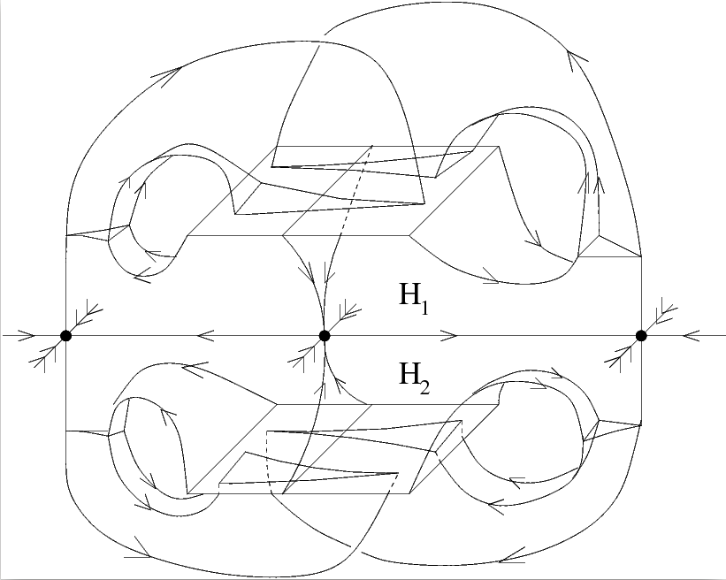
Figure 1. Example of a singular-hyperbolic attracting set, non-transitive and containing non-Lorenz like singularities.

In addition, recent results obtained in [9, 10] depend on the skew-product representation of a global Poincaré map given by Theorem 2.8 (corresponding to [9, Theorem 5] ensuring the application of [9, Theorem A and Proposition 1] to singular-hyperbolic attractors), which now holds without assuming transitivity or that all equilibria are non-resonant Lorenz-like singularities for $3$-dimensional vector fields only.

Hence, exponential decay of correlations for the physical measures of the Global Poincaré map together with exact dimensionality and the logarithm law for hitting times for the physical/SRB measures of the flow on $\Lambda$ [9, Corollaries 1 and 2] are true in the same setting of Theorem A.

1.3.1. Consequences for one-dimensional maps

In the statement of Theorem C we assume that

• each discontinuity point with finite lateral derivative (in ${\mathcal{D}}\setminus{\mathcal{S}}$) admits a one-sided neighborhood which is sent to a one-sided neighborhood of a singular point (in ${\mathcal{S}}$, a discontinuity point with unbounded lateral derivative) in a finite and uniformly bounded number of iterates;

• the set ${\mathcal{S}}$ is non-degenerate in the usual sense from one-dimensional dynamics [30] as in assumption (1.3), that is, $|f^{\prime}|$ grows as a power of the distance to ${\mathcal{S}}$ (see also e.g. the conditions on the critical/singular set in [31] for a similar statement in the $C^{2}$ setting).

Near singular points the rate of expansion is proportional to a power of the distance to the singularity, which allows distortion control. The coexistence of singularities and discontinuity points in the same map makes it more difficult to control distortion near the boundaries of the monotonicity intervals. The assumption that each point in ${\mathcal{D}}\setminus{\mathcal{S}}$ is eventually sent in ${\mathcal{S}}$ enables us to adapt the combinatorial method of proof from [7, Section 6] to this setting, which uses partition refinement techniques first developed in the works of Benedicks and Carleson [21, 22] later expanded in [50, 53, 45, 16].

Similar techniques were used by Freitas [33] applied to the quadratic family to obtain exponentially slow approximation to the critical point on Benedicks-Carleson parameters; and by Diaz-Ordaz, Holland and Luzzatto [31] to study one-dimensional $C^{2}$ maps with critical points or singularities.

In contrast to these works, where only one or finitely many criticalities and/or singularities were allowed and with no interaction between them, here we deal with a Hölder-$C^{1}$ map having non-degenerate singularities and criticalities and assume a strong interaction between them.

In most works seeking the construction of a Gibbs-Markov tower for non-uniformly expanding maps, asymptotic conditions on the recurrence to an exceptional subset (of criticalities, discontinuities or singularities) are assumed providing existence of hyperbolic times, which are endowed with automatic recurrence control to the singular/discontinuity set. This control however does not ensure specific rates of decay and other finer statistical properties, which are often stated conditionally on the class of decay rates (polynomial, super-polynomial, stretched exponential, exponential etc); e.g. [5, 4, 44, 34].

Here we want to deduce this asymptotic recurrence control from weaker assumptions on $f$, in a similar vein as [21, 22, 50, 53, 45] but in a much simpler setting, which then provides hyperbolic times and many strong statistical properties, as explained below.

However in [7] a problem with the bounded distortion argument was unfortunately overlooked: the derivative $f^{\prime}$ of the map $f$ (even in the case of the Lorenz map from the geometric Lorenz attractor) is not Hölder continuous on a whole one-sided neighborhood of the singularities, since $f^{\prime}$ is unbounded there. In fact, for $x,y\in\Delta(c,\delta_{c})$ near a singularity $c\in{\mathcal{S}}$ we have $|f^{\prime}x-f^{\prime}y|/|f^{\prime}x|\approx|x-y|/|x-c|$ from (1.3), so to be able to bound $|f^{\prime}x-f^{\prime}y|$ we need $|x-y|\approx|x-c|^{\theta}$ for some convenient $0<\theta<1$ and $x,y$ in the same atom of a convenient partition. But this is not provided by any exponential partition around the points of ${\mathcal{D}}$, even with polynomial refinement (since in this case $|x-y|/|x-c|\approx 1/|\log|x-c||$) as used in all the works [21, 22, 50, 53, 45] (and many others) related to the Benedicks-Carleson refinement technique.

We overcome this issue by changing the way the initial partition is chosen: the length of its elements (intervals) is comparable to a suitable power of the distance to ${\mathcal{D}}$ in order to ensure bounded distortion. However, we do not change the refinement strategy with respect to [7], but the finer details have been thoroughly presented in Section 4. To the best of the authors’ knowledge, this is the first time non-exponential initial partitions are used in this setting and still provide upper exponential decay for the Lebesgue measure of the deviations subset.

Applications of this result are given by singular-hyperbolic attracting sets as in Theorem A, where we reduce the analysis to a one-dimensional map with a finite singular/discontinuity subset ${\mathcal{D}}$; see Section 3. Coupling with well-known results on non-uniformly expanding maps we obtain results on existence of absolutely continuous invariant probability measures and its statistical properties.

We say that $f$ is non-uniformly expanding if there exists $c>0$ such that

$$\liminf_{n\to+\infty}\frac{1}{n}\sum_{j=0}^{n-1}\log|f^{\prime}(f^{j}x)|\geq c\quad{for}\quad\lambda-\text{a.e.}x.$$

This condition implies in particular that the lower Lyapunov exponent of the map $f$ is strictly positive Lebesgue almost everywhere.

Condition (1.5) implies that $S_{n}\Delta_{\delta}/n\to 0$ in measure, i.e., the map $f$ has slow recurrence to ${\mathcal{D}}$: for every $\varepsilon>0$ there exists $\delta>0$ such that

$$\limsup_{n\to\infty}\frac{1}{n}S_{n}\Delta_{\delta}(x)\leq\varepsilon\quad{for}\quad\lambda-\text{a.e.}x,$$

where from now on $S_{n}g(z)=S_{n}^{f}g(z)=\sum_{i=0}^{n-1}g(f^{i}z)$ denotes the ergodic sum of the function $g:Q\to{\mathbb{R}}$ with respect to $f$ in $n\geq 1$ iterates.

We note that from properties (1.3) and (1.4) together show that the singular set ${\mathcal{D}}$ is non-flat/non-degenerate similarly to the assumptions on [3]

These notions suitably generalized to an arbitrary dimensional setting were presented in [3] and in [3, 1] the following result on existence of finitely many absolutely continuous invariant probability measures was obtained.

Theorem 1.8 ([3, 1]).

Let $f:M\circlearrowleft$ be a $C^{2}$ local diffeomorphism outside a non-degenerate singular set ${\mathcal{D}}$. Assume that $f$ is non-uniformly expanding with slow recurrence to ${\mathcal{D}}$. Then there are finitely many ergodic absolutely continuous (in particular physical or Sinai-Ruelle-Bowen) $f$-invariant probability measures $\mu_{1},\dots,\mu_{k}$ whose basins cover the manifold Lebesgue almost everywhere, that is $B(\mu_{1})\cup\dots\cup B(\mu_{k})=M,\quad\operatorname{Leb}-\bmod 0$. Moreover the support of each measure contains an open disk in $M$.

Clearly, $f$ in the setting of Theorem C satisfies both the non-uniformly expanding and slow recurrence conditions. Moreover, considering the tail sets ${\mathcal{E}}(x)=\min\{N\geq 1:|(f^{n})^{\prime}(x)|>\sigma^{n/3},\forall n\geq N\}$ and ${\mathcal{R}}(x)=\min\{N\geq 1:S_{n}\Delta_{\delta}<\zeta n,\forall n\geq N\}$, the exponentially slow recurrence (1.5) can be translated as: there are constants $\delta,\zeta,C_{1},\xi>0$ so that

$$\lambda\Big{(}\{x\in I:{\mathcal{R}}(x)>n\}\Big{)}\leq C_{1}\cdot e^{-\xi_{1}\cdot n}\quad\text{for all}\quad n\geq 1;$$

and the uniform expanding assumption on $f$ means that there exist $\sigma>1$ and $N\in{\mathbb{Z}}^{+}$ so that $\{x\in I:{\mathcal{E}}(x)>n\}$ equals $I$ except finitely many points, for all $n>N$. Hence we have

$$\lambda\Big{(}\{x\in I:{\mathcal{R}}(x)>n\quad\text{and}\quad{\mathcal{E}}(x)>n\}\Big{)}\leq C_{1}\cdot e^{-\xi_{1}\cdot n}\quad\text{for all}\quad n\geq 1.$$ (1.7)

This allows us to deduce the following ergodic/statistical properties of $f$.

Corollary E.

Let $f$ be as in the statement of Theorem C. Then

1. ([3] and [5, Theorem 3]) there are finitely many absolutely continuous invariant probability measures $\mu_{1},\dots,\mu_{k}$ such that $B(\mu_{1})\cup\dots\cup B(\mu_{k})=M,\quad\lambda-\bmod 0$ and some finite power of $f$ is mixing with respect to $\mu_{i},i=1,\dots,k$;

2. [34] there exists an interval $Y_{i}$ with a return time function $R_{i}:Y_{i}\to{\mathbb{Z}}^{+}$ defining a Markov Tower over $f$ so that $\limsup\frac{1}{n}\log\mu_{i}\{R_{i}>n\}<0$ for each $i=1,\dots,k$;

3. ([5] and [34, Theorem 1.1]) there exist constants $C,c>0$ such that the correlation function $\mathrm{Corr}_{n}(\varphi,\psi)=\left|\int(\varphi\circ g^{n})\cdot\psi\,d\mu_{i}-\int\varphi\,d\mu_{i}\int\psi\,d\mu_{i}\right|,$ for Hölder continuous observables $\varphi,\psi:I\to{\mathbb{R}}$, satisfy $\mathrm{Corr}_{n}(\varphi,\psi)\leq C\cdot e^{-c\cdot n}$ for all $n\geq 1$ and each $i=1,\dots,k$;

4. [5, Theorem 4] $\mu_{i}$ satisfies the Central Limit Theorem: given a Hölder continuous function $\phi:I\to{\mathbb{R}}$ which is not a coboundary ($\phi\neq\psi\circ f-\psi$ for any continuous $\psi:I\to{\mathbb{R}}$) there exists $\theta>0$ such that for every interval $J\subset{\mathbb{R}}$ and each $i=1,\dots,k$

   $$\lim_{n\to\infty}\mu_{i}\Big{(}\Big{\{}x\in I:\frac{1}{\sqrt{n}}\sum_{j=0}^{n-1}\Big{(}\phi(f^{j}(x))-\int\phi d\mu_{i}\Big{)}\in J\Big{\}}\Big{)}=\frac{1}{\theta\sqrt{2\pi}}\int_{J}e^{-t^{2}/2\theta^{2}}dt.$$

5. [48, 35] For each $i=1,\dots,k$ let $\phi:I\to{\mathbb{R}}$ be a Hölder observable so that $\mu_{i}(\phi)=0$. Then $\phi$ satisfies the Almost Sure Invariance Principle: there exist $\varepsilon>0$, a sequence $S_{N}$ of random variables and a Brownian motion $W$ with variance $\sigma^{2}>0$ such that $\{\sum_{j=0}^{N-1}\phi\circ f^{j}\}=_{d}\{S_{N}\}$ and

   $$S_{N}=W(N)+O(N^{\frac{1}{2}-\varepsilon})\quad\text{as}\quad N\to\infty\quad\mu_{i}-\text{almost everywhere}.$$

Remark 1.9.

The Almost Sure Invariance Principle implies the Central Limit Theorem and also the functional CLT (weak invariance principle), and the law of the iterated logarithm together with its functional version, and many other results; see e.g. [58] for a comprehensive list.

1.3.2. Possible extensions and conjectures

A natural issue is whether is it possible to remove the assumption that ${\mathcal{S}}$ is nonempty or to relax the assumption that there are only finitely many discontinuity points all of which are sent to singular points in a uniformly bounded number of iterates.

Example with countable infinite ${\mathcal{D}}$

An example of a transformation with infinitely many monotonicity domains and ${\mathcal{S}}$ a single point, satisfying the conditions of Theorem C except that ${\mathcal{D}}$ is countably infinite, is given by a topologically exact Lorenz transformation in the interval $[f(0^{+}),f(0^{-})]$ strictly contained in $J=[-1/2,1/2]$ whose graph we complete as a function $J\to J$ with affine pieces between points having the same values of $f$ at some element of the preorbits of the unique singularity at $0$; see Figure 2.

Figure 2. Example of a piecewise expading maps with infinitely many branches in the setting of Theorem C but with an infinite ${\mathcal{D}}$.

We can perform this extension in a way that

• the slope of the affine branches be larger than $2$;

• the monotonicity domains form a denumerable partition of $J$;

• the singularity at $0$ is a Lorenz-like singularity which together with the discontinuity points for a non-degenerate singular set;

• every discontinuity point of the map is sent to $0$ in finitely many iterates and the orbit of the discontinuities up to arriving at $0$ forms a finite subset.

Conjecture 1.

Exponential slow recurrence to the singular/discontinuous set still holds in the setting of Theorem C with ${\mathcal{S}}=\emptyset$ and countably many discontinuities.

Extensions of Theorem A to the class of sectional-hyperbolic attracting sets for flows in higher dimensions, with dimension of the central direction higher than two, introduced by Metzger-Morales in [49], seem to involve subtle questions on the smoothness of the stable foliation of these sets which, on the one hand, might prevent the existence of a smooth quotient map of the Poincaré return map over the stable foliation in a natural way and, on the other hand, the dynamics of higher dimensional piecewise expanding maps is not so well understood as its one-dimensional couterpart, where the boundaries of the domains of smoothness have low complexity.

Conjecture 2.

Large deviations with respect to Lebesgue measure versus physical measures, for continuous observables on a neighborhood of general sectional-hyperbolic attracting sets for $C^{2}$ flows have exponential upper bound.

Another issue is regularity: what can we say about large deviations for singular-hyperbolic attracting sets of $C^{1}$ flows?

Conjecture 3.

The statements of Theorem A and Conjecture 2 are still valid for $C^{1}$ flows.

Using the existence of Markov towers with exponential tails for the one-dimensional map as in Corollary E it is natural to search for statistical properties for the flows in the setting of Theorem A along the lines of [14, 11, 12]. This will be done in a systematic way in [13].

1.4. Organization of the text

The proof of Theorem A demanded the extension of the construction of adapted cross-sections used in [18] for singular-hyperbolic attractors (i.e. transitive attracting sets) since the existence of a dense forward orbit inside the attracting set was crucial to find Poincaré sections whose boundaries are contained in stable manifolds of some singularity of the attracting set. Moreover, since we are not assuming the existence of a dense regular orbit, we need to consider the possible existence of singularities in the attracting set which are not Lorenz-like.

This construction, without the transitivity assumption, is presented in Section 2 were a global Poincaré map is built and Theorem 2.8 on the representation of this map as a skew-product over a one-dimensional transformation is proved.

The proof of item (1) of Theorem A follows from Theorem 2.8, whose proof is presented in Subsectionc 2.2, together with Theorem 1.7 presented in Subsection 1.3. The deduction of item (2) of Theorem A from the reduction to a one-dimensional transformation in the setting of Theorem C, following the route in [15, 7], is presented in Section 3 assuming the statement of Theorem C. Then Theorem C together with Corollary D are proved in Section 4.

Acknowledgments

We thank the referee for the careful reading of the manuscript and the many detailed questions which greatly helped to improve the statements of the results and the readability of the text.

This is the PhD thesis of A. Souza and part of the PhD thesis work of E. Trindade at the Instituto de Matemática e Estatística-Universidade Federal da Bahia (UFBA, Salvador) under a CAPES (Brazil) scholarship. Both thank the Mathematics and Statistics Institute at UFBA for the use of its facilities and the financial support from CAPES during their M.Sc. and Ph.D. studies.

2. Existence of adapted cross-sections and construction of global Poincaré map

We let $X\in{{\mathfrak{X}}}^{2}(M)$ admit an singular-hyperbolic attracting set $\Lambda=\bigcap_{t>0}\overline{X^{t}(U_{0})}$ for some open neighborhood $U_{0}$, with $DX^{t}$-invariant splitting $T_{\Lambda}M=E^{s}\oplus E^{cu}$, $d_{s}=\dim E^{s}=d-2$ and $d_{cu}=\dim E^{cu}=2$.

2.1. Properties of singular-hyperbolic attracting sets

We extend the stable direction on $\Lambda$ to a $DX^{t}$-invariant stable bundle over $U_{0}$ and then integrate these directions into a topological foliation of $U_{0}$ which admits Hölder-$C^{1}$ holonomies, combining the following results.

Proposition 2.1.

Let $\Lambda$ be a partially hyperbolic attracting set. The stable bundle $E^{s}$ over $\Lambda$ extends to a continuous uniformly contracting $DX^{t}$-invariant bundle $E^{s}$ over an open neighborhood of $\Lambda$.

Proof.

See [12, Proposition 3.2] and note [12, Remark 3.3] ensuring that the existence of this extension does not depend on transitivity. ∎

We assume without loss of generality that $E^{s}$ extends as in Proposition 2.1 to $U_{0}$.

Recall that $B^{k}$ is the $k$-dimensional open unit disk endowed with the Euclidean distance induced by the Euclidean norm $\|\cdot\|_{2}$, and let $\mathrm{Emb}^{2}(B^{k},M)$ denote the set of $C^{2}$ embeddings $\phi:B^{k}\to M$ endowed with the $C^{2}$ distance.

Proposition 2.2.

Let $\Lambda$ be a partially hyperbolic attracting set. There exists a positively invariant neighborhood $U_{0}$ of $\Lambda$, and constants $\lambda\in(0,1),c>0$, such that the following are true:

1. For every point $x\in U_{0}$ there is a $C^{2}$ embedded $d_{s}$-dimensional disk $W^{s}_{x}\subset M$, with $x\in W^{s}_{x}$, such that

   1. $T_{x}W^{s}_{x}=E^{s}_{x}$.

   2. $X^{t}(W^{s}_{x})\subset W^{s}_{X^{t}x}$ for all $t\geq 0$.

   3. $d(X^{t}x,X^{t}y)\leq c\lambda^{t}d(x,y)$ for all $y\in W^{s}_{x}$, $t\geq 0$.

2. The disks $W^{s}_{x}$ depend continuously on $x$ in the $C^{0}$ topology: there is a continuous map $\gamma:U_{0}\to{\rm Emb}^{0}(B^{d_{s}},M)$ such that $\gamma(x)(0)=x$ and $\gamma(x)(B^{d_{s}})=W^{s}_{x}$. Moreover, there exists $L>0$ such that $\operatorname{Lip}\gamma(x)\leq L$ for all $x\in U_{0}$.

3. The family of disks $\{W^{s}_{x}:x\in U_{0}\}$ defines a topological foliation of $U_{0}$.

Proof.

See [12, Theorem 4.2 and Lemma 4.8], where $\operatorname{Lip}\gamma(x)$ is the Lipschitz constant of $\gamma(x)$, given by $\sup\{\frac{\operatorname{dist}(\gamma(x)(u),\gamma(x)(v))}{\|u-v\|_{2}}:u\neq v,w,v\in B^{d_{s}}\}$. Note also that the results in [12, Section 4] do not use either transitivity or central volume expansion in its proofs, that is, these results hold for partial hyperbolic attracting sets. ∎

The splitting $T_{\Lambda}M=E^{s}\oplus E^{cu}$ extends continuously to a splitting $T_{U_{0}}M=E^{s}\oplus E^{cu}$ where $E^{s}$ is the invariant uniformly contracting bundle in Proposition 2.1 and, in general, $E^{cu}$ is not invariant. Given $a>0$, we consider the center-unstable cone field

$$\mathcal{C}^{cu}_{x}(a)=\{v=v^{s}+v^{cu}\in E^{s}_{x}\oplus E^{cu}_{x}:\|v^{s}\|\leq a\|v^{cu}\|\},\quad x\in U_{0}.$$

Proposition 2.3.

Let $\Lambda$ be a partially hyperbolic attracting set. There exists $T_{0}>0$ such that for any $a>0$, after possibly shrinking $U_{0}$,

$$DX^{t}\cdot\mathcal{C}^{cu}_{x}(a)\subset\mathcal{C}^{cu}_{X^{t}x}(a)\quad\text{for all $t\geq T_{0}$, $x\in U_{0}$}.$$

Proof.

See [12, Proposition 3.1] and again note that the results in [12, Section 3] do not use either transitivity or central volume expansion in its proofs. ∎

Proposition 2.4.

Let $\Lambda$ be a singular hyperbolic attracting set. After possibly increasing $T_{0}$ and shrinking $U_{0}$, there exist constants $K,\theta>0$ such that $|\det(DX^{t}|E^{cu}_{x})|\geq K\,e^{\theta t}$ for all $x\in U_{0}$, $t\geq 0$.

Proof.

See [13, Proposition 2.10] ∎

2.1.1. The stable lamination is a topological foliation

The Stable Manifold Theorem [65] ensures the existence of an $X^{t}$-invariant stable lamination ${\mathcal{W}}^{s}_{\Lambda}$ consisting of smoothly embedded disks $W^{s}_{x}$ through each point $x\in\Lambda$. Although not true for general partially hyperbolic attractors, for singular-hyperbolic attractors in our setting ${\mathcal{W}}^{s}_{\Lambda}$ indeed defines a topological foliation in an open neighborhood of $\Lambda$.

Theorem 2.5.

Let $\Lambda$ be a singular hyperbolic attracting set. Then the stable lamination ${\mathcal{W}}^{s}_{\Lambda}$ is a topological foliation of an open neighborhood of $\Lambda$.

Proof.

See [13, Theorem 5.1] where it is shown that ${\mathcal{W}}^{s}_{\Lambda}$ coincides with the topological foliation $\{W_{x}^{s}:x\in U_{0}\}$ of item (3) of Proposition 2.2. ∎

From now on, we refer to ${\mathcal{W}}^{s}=\{W^{s}_{x}:x\in\Lambda\}$ as the stable foliation.

2.1.2. Absolute continuity of the stable foliation

A key fact for us is regularity of stable holonomies. Let $Y_{0},\,Y_{1}\subset U_{0}$ be two smooth disjoint $d_{cu}$-dimensional disks that are transverse to the stable foliation ${\mathcal{W}}^{s}$. Suppose that for all $x\in Y_{0}$, the stable leaf $W^{s}_{x}$ intersects each of $Y_{0}$ and $Y_{1}$ in precisely one point. The stable holonomy $H:Y_{0}\to Y_{1}$ is given by defining $H(x)$ to be the intersection point of $W^{s}_{x}$ with $Y_{1}$.

Theorem 2.6.

The stable holonomy $H:Y_{0}\to Y_{1}$ is absolutely continuous. That is, $m_{1}\ll H_{*}m_{0}$ where $m_{i}$ is Lebesgue measure on $Y_{i}$, $i=0,1$. Moreover, the Jacobian $JH:Y_{0}\to\mathcal{R}$ given by

$$JH(x)=\frac{dm_{1}}{dH_{*}m_{0}}(Hx)=\lim_{r\to 0}\frac{m_{1}(H(B(x,r)))}{m_{0}(B(x,r))},\quad x\in Y_{0},$$

is bounded above and below and is $C^{\varepsilon}$ for some $\varepsilon>0$.

Proof.

This essentially follows from [19, Theorems 8.6.1 and 8.6.13] or from [57, Theorem 7.1] applied to $f=X^{T}$ for a large enough fixed $T>0$ which satisfies conditions (4.1), (4.2) and (4.3) of [57, Section 4] in the open positively invariant set $U$; see [13, Theorem 6.3]. ∎

Hence, we can assume without loss of generality, that there exists a foliation ${\mathcal{W}}^{s}$ of $U_{0}$, which continuously extends the stable lamination of $\Lambda$ together with a positively invariant field of cones $(\mathcal{C}^{cu}_{x})_{x\in U_{0}}$ on $T_{U_{0}}M$. Moreover, the Jacobian of holonomies along contracting leaves on cross-sections of singular-hyperbolic attracting sets in our setting is a Hölder function.

2.2. Global Poincaré return map

In [18] the construction of a global Poincaré map for any singular-hyperbolic attractor is carried out based on the existence of “adapted cross-sections” and Hölder-$C^{1}$ stable holonomies on these cross-sections. With the results just presented this construction can be performed for any singular-hyperbolic attracting set.

This construction was presented in [13, Sections 3 and 4]: we obtain

• a finite collection $\Xi=\Sigma_{1}+\dots+\Sigma_{m}$ of (pairwise disjoint) cross-sections to $X$ so that

  • each $\Sigma_{i}$ is diffeomorphically identified with $(-1,1)\times{\mathcal{D}}^{d_{s}}$;

  • the stable boundary $\partial^{s}\Sigma_{i}\cong\{\pm 1\}\times{\mathcal{D}}^{d_{s}}$ consists of two curves contained in stable leaves; and

  • each $\Sigma_{i}$ is foliated by $W^{s}_{x}(\Sigma_{i})=\bigcup_{|t|<\varepsilon_{0}}X^{t}(W^{s}_{x})\cap\Sigma_{i}$ for a small fixed $\varepsilon>0$. We denote this foliation by $W^{s}(\Sigma_{i}),i=1,\dots,m$;

• a Poincaré map $R:\Xi\setminus\Gamma\to\Xi$ which is $C^{2}$ smooth in $\Sigma_{i}\setminus\Gamma,i=1,\dots,m$; preserves the foliation $W^{s}(\Xi)$ and a big enough time $T>0$, where $\Gamma=\Gamma_{0}\cup\Gamma_{1}$ is a finite family of stable disks $W^{s}_{x_{i}}(\Xi)$ so that

  • $\Gamma_{0}=\{x\in\Xi:X^{T+1}(x)\in\bigcup_{\sigma\in S}\gamma^{s}_{\sigma}\}$ for $S=S(X,\Lambda)=\{\sigma\in\Lambda:X(\sigma)=\vec{0}\}$ and $\gamma_{\sigma}^{s}$ is the local stable manifold of $\sigma$ in a small fixed neighborhood of $\sigma\in S$; and

  • $\Gamma_{1}=\{x\in\Xi:R(x)\in\partial^{s}\Xi=\cup_{i}\partial^{s}\Sigma_{i}\}$

• and an open neighborhood $V_{0}$ of $S$ of so that every orbit of a regular point $z\in U_{0}\setminus V_{0}$ eventually hits $\Xi$ or else $z\in\Gamma$.

Having this, the same arguments from [18] (see [13, Proposition 4.1 and Theorem 4.3]) show that $DR$ contracts $T_{\Xi}W^{s}(\Xi)$ and expands vectors on the unstable cones $\{C^{u}_{x}(\Xi)=C^{cu}_{x}(a)\cap T_{x}\Xi\}_{x\in\Xi\setminus\Gamma}$. The stable holonomies for $R$ enable us to reduce its dynamics to a one-dimensional map, as follows.

Let $\gamma_{i}\subset\Sigma_{i}$ be curves that cross $\Sigma_{i}$, that is, $\dot{\gamma}_{i}\in C^{u}_{\gamma}$ and for all $x\in\Sigma_{i}$ the stable leaf $W^{s}_{x}(\Sigma_{i})$ intersects $\gamma_{i}$ in precisely one point, $i=1,\dots,m$. The (sectional) stable holonomy $h:\Xi\to\gamma=\sum_{i}\gamma_{i}$ is defined by setting $h(x)$ to be the intersection point of $W^{s}_{x}(\Sigma_{i})$ with $\gamma_{i}$, $x\in\Sigma_{i},i=1,\dots,m$.

Lemma 2.7.

The stable holonomy $h$ is $C^{1+\varepsilon}$ for some $\varepsilon>0$.

Proof.

See [13, Lemma 7.1] ∎

Following the same arguments in [18] (see also [13, Section 7]) we obtain a one-dimensional piecewise $C^{1+\alpha}$ quotient map over the stable leaves $f:\gamma\setminus\Gamma\to\gamma$ for some $0<\alpha<1$ so that $h(Rx)=f(x)$ and $|f^{\prime}x|>2$. Choosing smooth parametrizations of $\gamma_{i}$ in a concatenated fashion we can write $I=I_{1}\cup\dots\cup I_{m}$ and $f:I\setminus{\mathcal{D}}\to I$ where ${\mathcal{D}}$ is a finite set of points identified with $h(\Gamma)$ and each $I_{i}$ is identified with $\gamma_{i},i=1,\dots,m$. In addition, as shown in [13, Proof of Lemma 8.4], $|f^{\prime}\mid_{I\setminus{\mathcal{D}}}|$ behaves near singular points ${\mathcal{S}}$, identified with $h(\Gamma_{0})$ as a subset of ${\mathcal{D}}$, as a power of the distance to ${\mathcal{S}}$, as in assumption of the statement of (1.3).

We can use the choice of coordinates and concatenation defining $I$ from $\gamma=\sum_{i}\gamma_{i}$ to choose coordinates in $\Xi=\sum_{i}\Sigma_{i}$ so that: $\Xi$ can be identified with $I\times B^{d_{s}}$; and each $\Sigma_{i}$ with $I_{i}\times B^{d_{s}},i=1,\dots,m$.

This construction can be summarized as in [9, Theorem 5] as follows, with adaptations to our more general setting: items (1-5) can be found in [18] but item (6), which is crucial for us, will be obtained in Remark 2.16 following Corollary 2.15 in Subsection 2.4.3. This is the only argument where the assumption of connectedness is used; see [12, 13].

In what follows, we say that a function $\varphi:\Xi_{0}=\Xi\setminus\Gamma\to{\mathbb{R}}$ has logarithmic growth near $\Gamma$ if there is $K=K(\varphi)>0$ so that $|\varphi|\chi_{B(\Gamma,\delta)}\leq K\Delta_{\delta}\circ h$ for every small enough $\delta>0$.

Theorem 2.8.

[9, Theorem 5, Section 4, p 1021] For a $C^{2}$ vector field $X$ on a compact manifold having a connected singular hyperbolic attracting set $\Lambda$, there exists $\alpha>0$ and a finite family $\Xi$ of adapted cross-sections and a global Poincaré map $R:\Xi_{0}\to\Xi$, $R(x)=X^{\tau(x)}(x)$ such that

1. the domain $\Xi_{0}=\Xi\setminus\Gamma$ is the entire cross-sections with a family $\Gamma$ of finitely many smooth arcs removed and

   1. $\tau:\Xi_{0}\to[\tau_{0},+\infty)$ is a smooth function with logarithmic growth near $\Gamma$ and bounded away from zero by some uniform constant $\tau_{0}>0$;

   2. there exists a constant $\kappa>0$ so that $|\tau(y)-\tau(w)|<\kappa\operatorname{dist}(y,w)$ for all points $w\in W^{s}(y,\Xi)$ in the stable leaf through a point $y$ inside a cross-section of $\Xi$;

2. We can choose coordinates on $\Xi$ so that the map $R$ can be written as $F:\tilde{Q}\to Q$, $F(x,y)=(f(x),g(x,y))$, where $Q=I\times B^{d_{s}}$, $I=[0,1]$ and $\tilde{Q}=Q\setminus\tilde{\Gamma}$ with $\tilde{\Gamma}={\mathcal{D}}\times B^{d_{s}}$ and ${\mathcal{D}}=\{c_{1},\dots,c_{n}\}\subset I$ a finite set of points.

3. The map $f:I\setminus{\mathcal{D}}\to I$ is a piecewise $C^{1+\alpha}$ map of the interval with finitely many branches defined on the connected components of $I\setminus{\mathcal{D}}$ and has a finite set of ergodic a.c.i.m. $\mu^{i}_{f},i=1,\dots,k$ whose ergodic basins cover $I$ Lebesgue modulo zero. Also

   1. $\inf\{|f^{\prime}x|:x\in I\setminus{\mathcal{D}}\}>2$;

   2. the elements $c$ of ${\mathcal{D}}$ have a one-sided critical order $0<\alpha(c^{\pm})\leq 1$ as in (1.3);

   3. $1/|Df|$ has universal bounded $p$-variation; and

   4. $d\mu^{i}_{f}/dm$ has bounded $p$-variation for some $p>0$.

4. The map $g:\tilde{Q}\to B^{d_{s}}$ preserves and uniformly contracts the vertical foliation ${\mathcal{F}}=\{\{x\}\times B^{d_{s}}\}_{x\in I}$ of $Q$: there exists $0<\lambda<1$ such that $\operatorname{dist}(g(x,y_{1}),g(x,y_{2}))\leq\lambda\cdot|y_{1}-y_{2}|$ for each $y_{1},y_{2}\in B^{d_{s}}$.

5. The map $F$ admits a finite family of physical ergodic probability measures $\mu^{i}_{F}$ which are induced by $\mu^{i}_{f}$ in a standard way. The Poincaré time $\tau$ is integrable both with respect to each $\mu^{i}_{f}$ and with respect to the two-dimensional Lebesgue area measure of $Q$.

6. The subset ${\mathcal{S}}=\{c\in{\mathcal{D}}:0<\alpha(c)<1\}$ is nonempty and satisfies $\exists T_{0}\in{\mathbb{Z}}^{+}\,\forall c\in{\mathcal{D}}\setminus{\mathcal{S}}\,\exists T=T(c)\leq T_{0}$ so that $f^{T}(c)\in{\mathcal{S}}$, $\forall 0<j<T\exists c_{j}\in{\mathcal{D}}\setminus{\mathcal{S}}:f^{j}(c)\in\Delta(c_{j},\delta_{c_{j}})$, and we can find $\varepsilon,\delta>0$ such that $f\mid_{\Delta(c,\delta)}$ is a diffeomorphism into $\Delta(f^{T}(c),\varepsilon)$. Moreover

   1. $c\in{\mathcal{S}}\ \iff\lim_{t\to c}|t-b|^{1-\alpha(c)}\cdot|f^{\prime}(t)|$ exists and is finite;

   2. $c\in{\mathcal{D}}\setminus{\mathcal{S}}\iff$ the limit $\lim_{t\to c}|f^{\prime}(t)|$ exists and is finite.

Remark 2.9.

Due to the dimension and codimension of ${\mathcal{D}}$ as a submanifold of the quotient $I=\Xi/W^{s}(\Xi)$ together with logarithmic growth of $\tau$ near $\Gamma$, there exists $C_{d},d>0$ such that for all small $\rho>0$ $\operatorname{Leb}\{x\in M:\operatorname{dist}(x,{\mathcal{D}})<\rho\}\leq C_{d}\rho^{d},$ that is, the Lebesgue measure of neighborhoods of ${\mathcal{D}}$ is comparable to a power of the distance to ${\mathcal{D}}$. In our sectional-hyperbolic case $d=1$.

2.3. Equivalence between SRB/physical measure and equilibrium state

We now prove Theorem 1.7 showing that in singular-hyperbolic attracting sets for a $C^{2}$ smooth flow we can characterize physical/SRB measures in the same way as in hyperbolic attracting sets.

Proof of Theorem 1.7.

Let $\mu$ be a $X$-invariant probability measure supported in the singular-hyperbolic attracting set $\Lambda$.

We start by recalling that from Theorem 2.8 we can follow [18, Sections 6-8] to obtain (1.6). More precisely: the arguments in [18, Sections 6-8] show that from the existence of a finite family $\Xi$ of adapted cross-sections and a global Poincaré map satisfying items (1-5) of Theorem 2.8, we induce finitely many physical/SRB ergodic probability measures $\mu_{1},\dots,\mu_{k}$ for the flow (one for each measure $\mu_{i}^{f}$ given in Theorem 2.8) whose ergodic basins cover the trapping region of the attracting set $\Lambda$ and if, in addition, $\Lambda$ is transitive, then these ergodic physical measures cannot be distinct; for this final reasoning see [18, Subsection 7.1]. This proves item (1) of the statement of Theorem 1.7.

To prove item (2), we note that, since (i) $\int\log|\det DX^{1}\mid_{E^{cu}}|\,d\mu_{i}>0$ by singular-hyperbolicity, (ii) each $\mu_{i}$ is an ergodic physical/SRB measure, (iii) the Lyapunov exponent along the direction of the flow is zero and (iv) this direction is contained in the central direction then, by the characterization of measures satisfying the Entropy Formula [43], we get

$$h_{\mu_{i}}(X^{1})=\int\lambda^{+}(x)\,d\mu_{i}(x)=\int\log|\det DX^{1}\mid_{E^{cu}}|\,d\mu_{i}$$ (2.1)

where $\lambda^{+}(x)$ is the positive Lyapunov exponent along the orbit of $x\in\Lambda$ in the direction of $E^{cu}_{x}$. That is, each $\mu_{i}$ satisfies property (a): it is an equilibrium state with respect to the central Jacobian, $i=1,\dots,k$.

We now prove the implication $(c)\implies(a)$.

If the basin $B(\mu)$ of $\mu$ has positive Lebesgue measure, then by invariance $B(\mu)\cap U$ must have positive Lebesgue measure. So we get a Lebesgue modulo zero decomposition $B(\mu)\cap U=U\cap\big{(}\sum_{i=1}^{k}B(\mu)\cap B(\mu_{i})\big{)}$. By definition of physical measure, this means that for each continuous observable $\varphi:U\to{\mathbb{R}}$

$$\int\varphi\,d\mu =\frac{1}{\operatorname{Leb}(U)}\int_{U}\int\varphi\,d\left(\lim_{n\to+\infty}\frac{1}{n}\sum_{j=0}^{n-1}\delta_{f^{j}x}\right)\,d\operatorname{Leb}(x)$$

$$=\sum_{i=1}^{k}\frac{\operatorname{Leb}(B(\mu)\cap B(\mu_{i})\cap U)}{\operatorname{Leb}(U)}\int\varphi\,d\mu_{i},$$

where the limit above is in the weak^∗ topology of the probability measures of the manifold. Hence, we obtain $\mu=\sum_{i=1}^{k}\frac{\operatorname{Leb}(B(\mu)\cap B(\mu_{i})\cap U)}{\operatorname{Leb}(U)}\mu_{i}$ and $\mu$ is a convex linear combination of the ergodic physical/SRB measures provided by item (1). In particular, $\mu=\mu_{i}$ for some $i\in\{1,\dots,k\}$ by ergodicity and $\mu$ is a equilibrium state with respect to the central Jacobian.

Next we prove that $(a)\implies(b)\implies(c)$. The assumption (a) implies, since $\mu$ is ergodic, the Lyapunov exponent along the flow direction is zero and this direction is contained in the two-dimensional central direction, that is, (2.1) is true for $\mu$ in the place of $\mu_{i}$.

Hence, by the work of Ledrappier [41, Theorem 2,7], we conclude that $\mu$ is a $SRB$ measure: $\mu$ has absolutely continuous disintegration along unstable manifolds $W^{u}(x)$ for $\mu$-a.e. $x\in\Lambda$ if the Entropy Formula (2.1) holds. Hence, by invariance of the unstable manifolds and smoothness of the flow, we see that $\mu$ has absolutely continuous disintegration along the central-unstable manifolds $W^{cu}(x)$ for $\mu$-a.e. $x$, where $W^{cu}(x)=\cup_{t\in{\mathbb{R}}}X_{t}W^{u}(x)$. This shows that $(a)\implies(b)$.

Let $\Lambda_{1}$ be a full $\mu$-measure subset of $\Lambda$ where the previous absolutely continuous disintegration property holds. Since $\Lambda$ is a attracting set, then $\Lambda$ contains all unstable manifolds and so all the central-unstable manifolds $W^{cu}(x)$ for $x\in\Lambda_{1}$. We recall that $W^{cu}(x)$ is tangent to $E^{c}(x)$ at $x\in\Lambda_{1}$.

In addition, because $\Lambda$ has a partially hyperbolic splitting, every point $y$ of $\Lambda$ admits a stable manifold $W^{s}(y)$ which is tangent to $E^{s}(y)$ at $y$. Thus $W^{s}(y)$ are transverse to $W^{cu}(x)$ for all $y\in W^{cu}(x)$ and $x\in\Lambda_{1}$.

Moreover, the future time averages of $z\in W^{s}(y)$ and $y$ are the same for all continuous observables. Also, the future time averages of $y\in A_{x}\subset W^{u}(x)$ and $x$ are the same for all continuous observables and some subset $A_{x}$ of $W^{cu}(x)$ with positive area (by the absolutely continuous disintegration) for each $x\in\Lambda_{1}$. Hence the subset

$$B=\{W^{s}(y):y\in A_{x},x\in\Lambda_{1}\}$$

is contained in the ergodic basin of the measure $\mu$.

For $C^{2}$ smooth partially hyperbolic flows it is well-known that the strong-stable foliation $\{W^{s}(x)\}_{x\in\Lambda}$ is an absolutely continuous foliation of $U$; recall Theorem 2.6 and see [57]. In particular, the set $B$ has positive Lebesgue measure. Hence $\operatorname{Leb}(B(\mu))\geq\operatorname{Leb}(B)>0$ and $\mu$ is a physical measure.

This shows that $(b)\implies(c)$ and completes the proof of item (2).

Finally, the characterization of ${\mathbb{E}}$ is a consequence of the equivalence obtained in item (2): using Ergodic Decomposition [46] applied to both sides of the Entropy Formula

$$h_{\mu}(X^{1}) =\int\log|\det DX^{1}\mid_{E^{cu}}|\,d\mu\iff$$

$$\int h_{\mu_{x}}(X^{1})\,d\mu(x) =\int\int\log|DX^{1}\mid_{E^{cu}}|\,d\mu_{x}\,d\mu(x)$$

together with Ruelle’s Inequality $h_{\mu_{x}}(X^{1})\leq\int\log|DX^{1}\mid_{E^{cu}}|\,d\mu_{x}$ ensures that $\mu_{x}\in{\mathbb{E}}$ for $\mu$-a.e $x$ and so $\mu_{x}=\mu_{i(x)}$ for some $i(x)\in\{1,\dots,k\}$, since $\mu_{x}$ is ergodic for $\mu$-a.e. $x$. Thus $\mu$ is a linear convex combination of $\mu_{1},\dots,\mu_{k}$, completing the proof of item (3). ∎

2.4. Density of stable manifolds of singularities

The following is essential to obtain the property in item (6) of Theorem 2.8.

From Subsection 2.2 the one-dimensional map $f:I\setminus{\mathcal{D}}\to I$ can be written $f:\sum_{j}I_{j}\to I:=\overline{\sum_{j}I_{j}}$, where the $I_{j}$ are the finitely many connected components of $I\setminus{\mathcal{D}}$ (that is, open subintervals).

2.4.1. Topological properties of the dynamics of $f$

The following provides the existence of a special class of periodic orbits for $f$.

Proposition 2.10.

Let $f:\sum_{j}I_{j}\to I$ be a piecewise $C^{1}$ expanding map with finitely many branches $I_{1},\dots,I_{l}$ such that each $I_{j}$ is a non-empty open interval, $|Df\mid I_{j}|\geq\sigma>2$ and $I\setminus(\sum_{j}I_{j})$ is finite.

Then, for each small $\delta>0$ there exists $n=n(\delta)$ such that, for every non-empty open interval $J\subset\sum_{j}I_{j}$ with $|J|\geq\delta$, we can find $0\leq k\leq n$, a sub-interval $\hat{J}$ of $J$ and $1\leq j\leq l$ satisfying

$$f^{k}\mid\hat{J}:\hat{J}\to I_{j}\quad\text{is a diffeomorphism}.$$

In addition, $f$ admits finitely many periodic orbits ${\mathcal{O}}(p_{1}),\dots,{\mathcal{O}}(p_{k})$ contained in $\sum_{j}I_{j}$ with the property that every non-empty open interval $J\subset\sum_{j}I_{j}$ admits an open sub-interval $\hat{J}$, a periodic point $p_{j}$ and an iterate $n$ such that $f^{n}\mid\hat{J}$ is a diffeomorphism onto a neighborhood of $p_{j}$.

Proof.

See [17, Lemma 6.30]. ∎

Remark 2.11.

1. For the bidimensional map $F$ this shows that there are finitely many periodic orbits ${\mathcal{O}}(P_{1}),\dots,{\mathcal{O}}(P_{k})$ for $F$ so that $\pi({\mathcal{O}}(P_{i}))={\mathcal{O}}(p_{i}),i=1,\dots,k$, where $\pi:Q\to I$ is the projection on the first coordinate. Moreover, the union of the stable manifolds of these periodic orbits is dense in $Q$. See [17, Section 6.2] for details.

2. This also implies that the stable manifolds of the periodic orbits $P_{i}$ obtained above are dense in a neighborhood $U_{0}$ of $\Lambda$.

   Indeed, we can write the flow $X_{t}$ on a neighborhood of $\Lambda$ as a suspension flow over $F$; see [18]. Then the orbit of each $P_{i}$ is periodic and hyperbolic and $W^{s}_{G}(P_{i})$ is the suspension of $W^{s}_{F}(P_{i})$. Therefore, the density of $\cup_{i}W^{s}_{F}(P_{i})$ in $Q$ implies the density of $\cup_{i}W^{s}_{G}(P_{i})$ in a neighborhood $U_{0}$ of $\Lambda$.

2.4.2. Ergodic properties of $f$

The map $f$ is piecewise expanding with Hölder derivative which enables us to use strong results on one-dimensional dynamics.

Existence and finiteness of acim’s

It is well known [36] that $C^{1}$ piecewise expanding maps $f$ of the interval such that $1/|Df|$ has bounded variation have absolutely continuous invariant probability measures whose basins cover Lebesgue almost all points of $I$.

Using an extension of the notion of bounded variation this result was extended in [39] to $C^{1}$ piecewise expanding maps $f$ such that $g=1/|f^{\prime}|$ is $\alpha$-Hölder for some $\alpha\in(0,1)$. In addition from [39, Theorem 3.3] there are finitely many ergodic absolutely continuous invariant probability measures $\upsilon_{1},\dots,\upsilon_{l}$ of $f$ and every absolutely continuous invariant probability measure $\upsilon$ decomposes into a convex linear combination $\upsilon=\sum_{i=1}^{l}a_{i}\upsilon_{i}$. From [39, Theorem 3.2] considering any subinterval $J\subset I$ and the normalized Lebesgue measure $\lambda_{J}=(\lambda\mid J)/\lambda(J)$ on $J$, every weak^∗ accumulation point of $n^{-1}\sum_{j=0}^{n-1}f_{*}^{j}(\lambda_{J})$ is an absolutely continuous invariant probability measure $\upsilon$ for $f$ (since the indicator function of $J$ is of generalized $1/\alpha$-bounded variation). Hence the basin of the $\upsilon_{1},\dots,\upsilon_{l}$ cover $I$ Lebesgue modulo zero: $\lambda\big{(}I\setminus(B(\upsilon_{1})+\dots+B(\upsilon_{l})\big{)}=0.$

Note that from [39, Lemma 1.4] we also know that the density $\varphi$ of any absolutely continuous $f$-invariant probability measure is bounded from above.

Absolutely continuous measures and periodic orbits

Now we relate some topological and ergodic properties.

Lemma 2.12.

For each periodic orbit ${\mathcal{O}}(p_{i})$ of $f$ given by Proposition 2.10, there exists some ergodic absolutely continuous $f$-invariant probability measure $\upsilon_{j}$ such that $p_{i}\in\operatorname{supp}\upsilon_{j}$, and vice-versa.

Proof.

Define $E=\{1\leq i\leq k:\exists 1\leq j\leq l$ s.t. ${\mathcal{O}}(p_{i})\in\operatorname{supp}\upsilon_{j}\}$. Note that since $\operatorname{int}(\operatorname{supp}\upsilon_{1})$ is nonempty, then for an interval $J\subset\operatorname{int}(\operatorname{supp}\upsilon_{1})$ we can by Proposition 2.10 find another interval $\hat{J}\subset J$ and $n>1$ so that $f^{n}\mid_{\hat{J}}:\hat{J}\to V(p_{i})$ is a diffeomorphism to a neighborhood $V(p_{i})$ of $p_{i}$, for some $1\leq i\leq k$. The invariance of $\operatorname{supp}\upsilon_{1}$ shows that $p_{i}\in\operatorname{int}(\operatorname{supp}\upsilon_{1})$ and $E\neq\emptyset$.

We set $B=\{1,\dots,k\}\setminus E$ and show that $B=\emptyset$. For that, we write $i\to j$ if the preorbit of ${\mathcal{O}}(p_{j})$ accumulates ${\mathcal{O}}(p_{i})$.

Claim 2.13.

If $i\to j$ and $j\in E$, then $i\in E$.

Hence orbits in $B$ cannot link to orbits in $E$. Since the union of the preorbits of ${\mathcal{O}}(p_{i})$ are dense in $I$, then $B$ can only be accumulated by preorbits of elements of $B$. Thus, the union $W$ of the preorbits of the elements of $B$ is $f$-invariant and dense in a neighborhood of the orbits of the elements of $B$. Therefore, $\overline{W}$ is a compact $f$-invariant set with nonempty interior of $I$ and so $\overline{W}$ contains the support of some $\upsilon_{j}$. Consequently, the preorbit of some element of $B$ intersects $\operatorname{int}(\operatorname{supp}\upsilon_{j})$ and so $B\cap E\neq\emptyset$. This contradiction proves that $B$ must be empty, except for the proof of the claim.

Proof of Claim 2.13.

There exists $x_{n}\xrightarrow[n\to\infty]{}p_{i}$ so that $x_{n}\in\cup_{m\geq 0}f^{-m}p_{j}$ and then we can find $V_{n}$ neighborhood of $x_{n}$ and $m_{n}>1$ such that $f^{m_{n}}\mid_{V_{n}}:V_{n}\to V(p_{i})$ is a diffeomorphism onto a neighborhood $V(p_{j})$ of $p_{j}$.

But $V(p_{j})\cap\operatorname{supp}\upsilon_{h}\neq\emptyset$ for some $1\leq h\leq l$ and so, by invariance of $\operatorname{supp}\upsilon_{h}$, there are points of $\operatorname{supp}\upsilon_{h}$ in $V_{n}$, for all $n\geq 1$. This shows that $p_{i}$ is a limit point of $\operatorname{supp}\upsilon_{h}$, and so $i\in E$. This proves the claim and finishes the proof of the lemma. ∎

∎

2.4.3. Stable manifolds of singularities

We are now ready to obtain the property in item (6) of Theorem 2.8.

Theorem 2.14.

The union of the stable manifolds of the singularities in a connected singular-hyperbolic attracting set is dense in the topological basin of attraction, that is

$$U_{0}\subset\overline{\bigcup_{\sigma\in\Lambda\cap S(G)}W^{s}(\sigma)}$$

We present a proof of Theorem 2.14 in Subsection 2.4.4.

One important consequence is the possibility of choosing adapted cross-sections with a special feature crucial to obtain item (6) of the statement of Theorem 2.8.

Corollary 2.15.

Every regular point of a connected singular-hyperbolic attracting set admits cross-sections with arbitrarily small diameter whose stable boundary is formed by stable manifolds of singularities of the set, for every small enough $\delta>0$.

Proof.

Since there is a dense subset of stable leaves in $U_{0}$ that are part of $W^{s}(S)=\bigcup_{\sigma\in S}W^{s}(\sigma)$, we can choose a cross-section $\Sigma$ to $X$ at any point $x\in U_{0}$ with diameter as small as we like having a stable boundary contained in $W^{s}(S)$. ∎

Remark 2.16.

As a consequence of Corollary 2.15, the one-dimensional map $f$ satisfies item (6) of Theorem 2.8.

Indeed, points in the stable manifold of a singularity $\sigma\in\Lambda$ are sent in finite positive time by the flow to the local stable manifold of the singularity in a cross-section close to the singularity. We can also ensure that orbits of such stable boundaries do not contain stable boundaries of other cross-sections. For the one-dimensional map the corresponding behavior is precisely given by item (6) of Theorem 2.8.

Items (6a-6b) are consequences of the properties of $f$; see [13, Proof of Lemma 8.4] for more details. Moreover, we can assume that all singular points of $f$ are related to Lorenz-like singularities, after Remark 1.5.

2.4.4. Density of stable manifolds of singularities

To prove Theorem 2.14 we use non-uniform hyperbolic theory through the following result.

Theorem 2.17.

Let $\mu$ be an ergodic $f$-invariant hyperbolic probability measure supported in a connected singular-hyperbolic attracting set $\Lambda$.

Let us assume that $\mu$ is a $u$-Gibbs state, that is, for $\mu$-a.e. $x$ the unstable manifold $W^{u}_{x}$ is well-defined and Lebesgue-a.e. $y\in W^{u}_{x}$ is $\mu$-generic: $\frac{1}{T}\int_{0}^{T}\delta_{X_{s}y}\,ds\xrightarrow[T\to\infty]{w^{*}}\mu$.

Then there exists $\sigma\in S$ such that $W^{u}(p)\pitchfork W^{s}(\sigma)\neq\emptyset$ for every $p\in\operatorname{supp}\mu$.

We prove Theorem 2.17 in Subsection 2.4.5 and, based on this result, we can now present the following.

Proof of Theorem 2.14.

This theorem really is a corollary of Theorem 2.17 since we already know that the stable manifolds of the periodic orbits ${\mathcal{O}}(p_{i})$ are dense in a neighborhood $U_{0}$ of $\Lambda$; see Remark 2.11(2). The transverse intersection provided by Theorem 2.17 ensures, through the Inclination Lemma, that each of these stable manifolds is accumulated the stable manifold of some singularity, and the statement of Theorem 2.14 follows. ∎

2.4.5. Transversal intersection between unstable manifolds of periodic orbits and stable manifolds of singularities

The proof of Theorem 2.17 is based on a few results.

In what follows, we say that a disk $\gamma\subset M$ is a (local) strong-unstable manifold, or a strong-unstable manifold, if $\operatorname{dist}(X_{-t}(x),X_{-t}(y))$ tends to zero exponentially fast as $t\to+\infty$, for every $x,y\in\gamma$. It is well-know [38, 55] that every point $x$ of a hyperbolic periodic orbit ${\mathcal{O}}_{X}(p)$ for a vector field $X$ admits a local strong-unstable manifold which is an embedded disk tangent at $x\in{\mathcal{O}}_{X}(p)$ to the unstable direction $E^{u}_{x}$.

Considering the action of the flow we get the (global) strong-unstable manifold

$$W^{uu}(x)=\bigcup_{t>0}X_{t}\Big{(}W^{uu}_{loc}\big{(}X_{-t}(x)\big{)}\Big{)}$$

for every point $x$ of a uniformly hyperbolic set: in particular, for a hyperbolic periodic orbit ${\mathcal{O}}(p)$ of the flow of $X$.

In the present setting, since the singular-hyperbolic attracting set $\Lambda$ has codimension $2$ and the central direction $E^{c}_{\Lambda}$ contains the flow direction, then every periodic orbit ${\mathcal{O}}_{X}(p)$ in $\Lambda$ is hyperbolic and its unstable direction is one-dimensional. Hence the strong-unstable manifold through any point $x\in{\mathcal{O}}_{X}(p)$ is an immersed curve.

Lemma 2.18.

In the setting of the statement of Theorem 2.17, fix $p_{0}\in\operatorname{Per}(X)\cap\operatorname{supp}\mu$ and let $J=[a,b]$ be an arc on a connected component of $W^{uu}(p_{0})\setminus\{p_{0}\}$ with $a\neq b$. Then $H=\overline{\cup_{t>0}X^{t}(J)}$ contains some singularity of $\Lambda$.

Proof.

It is well-known from the non-uniform hyperbolic theory (Pesin’s Theory) that the support of a non-atomic hyperbolic ergodic probability measure $\mu$ is contained in a homoclinic class of a hyperbolic periodic orbit ${\mathcal{O}}(p)$; see e.g. [38, Appendix] or [20].

Hence, for $\mu$-a.e. $x$ we have $W^{u}_{x}\subset\operatorname{supp}\mu$ (since $\mu$ is a $u$-Gibbs measure) and $W^{u}_{x}\pitchfork W^{s}({\mathcal{O}}(p))\neq\emptyset$. Thus by the Inclination Lemma (see [54]) we have $W^{u}(p)\subset\overline{W^{u}(x)}\subset\operatorname{supp}\mu$.

Since every periodic point $p_{0}\in\operatorname{supp}\mu$ is homoclinically related to $p$ (that is, $W^{s}(p)\pitchfork W^{u}(p_{0})\neq\emptyset\neq W^{s}(p_{0})\pitchfork W^{u}(p)$), then we also have $W^{uu}(p_{0})\subset W^{u}(p_{0})\subset\operatorname{supp}\mu$.

Note that $H\subset\overline{W^{u}_{0}(p_{0})}\subset\operatorname{supp}\mu$ and $H$ is a compact invariant set by construction, where $W^{u}_{0}(p_{0})$ is the connected component of $W^{u}(p_{0})\setminus{\mathcal{O}}(p_{0})$ containing $J$. In addition, $H$ is clearly connected, since $H$ is also the closure of the orbit of the connected set $J$ under a continuous flow.

If $H$ has no singularities, then $H$ is a compact connected hyperbolic set and so contains the strong-unstable manifolds through any of its points, since every point in $H$ is accumulated by forward iterates of the arc $J$. This means that $H$ is an attracting set and so $H=\Lambda$ by connectedness, and $H$ contains all singularities of $\Lambda$. This contradiction proves that $H$ must contain a singularity. ∎

Fix $p_{0}$ and $\sigma\in S\cap H$ as in the statement of Lemma 2.18. We have shown that there exists $\sigma\in\operatorname{supp}\mu\cap S$ so that $\sigma\in\overline{W^{u}(p_{0})}$. We assume that $J$ is a fundamental domain for $W^{u}(p_{0})$, that is, $b=X^{T}(a)$ with $T>0$ the first return time of the orbit of $a$ to $W^{uu}(p_{0})$, i.e., $X^{t}(a)\notin W^{uu}(p_{0})$ for all $0<t<T$. We now argue just as in [17, Section 6.3.2, pp 199-202] and show that there exists some singularity whose stable manifold transversely intersects $J$.

This is enough to conclude the proof of Theorem 2.17. Indeed, since all periodic orbits in $\operatorname{supp}\mu$ are homoclinically related, it is enough to obtain $W^{u}(p_{0})\pitchfork W^{s}(\sigma)\neq\emptyset$ for a periodic point $p_{0}\in\operatorname{supp}\mu$.

To complete the argument, since in [17, Section 6.3.2] it was assumed that $\Lambda$ was either a singular-hyperbolic attractor or attracting set with dense periodic orbits for a $3$-vector field, we state [17, Lemma 6.49] in our setting.

Lemma 2.19.

Let $\tilde{\Sigma}$ be a cross-section of $X$ containing a compact $cu$-curve $\zeta$, which is the image of a regular parametrization $\zeta:[0,1]\to\tilde{\Sigma}$, and assume that $\zeta$ is contained in $\operatorname{supp}\mu$. Let $\Sigma$ be another cross-section of $X$. Suppose that $\zeta$ falls off $\Sigma$, that is

1. the positive orbit of $\zeta(t)$ visits $\operatorname{int}(\Sigma)$ for all $t\in[0,1)$;

2. and the $\omega$-limit of $\zeta(1)$ is disjoint from $\Sigma$.

Then $\zeta(1)$ belongs either to the stable manifold of some periodic orbit $p$ in $\operatorname{supp}\mu$, or to the stable manifold of some singularity.

Proof.

Just follow the same arguments in the proof of [17, Lemma 6.49] since the proof assumes that stable manifolds of the flow intersected with cross-sections disconnect the cross-sections (that is, the transverse intersection is a hypersurface inside the cross-section); and either the existence of a dense regular orbit, or the denseness of periodic orbits, each of which is true in the invariant subset $\operatorname{supp}\mu$ in our setting. ∎

3. Dimensional reduction of large deviations subset

Here we explain how to use the representation of the global Poincaré map obtained in Subsection 2.2 to reduce the problem of estimating an upper bound for the large deviations subset of the flow to a similar problem for a expanding quotient map on the base dynamics of a suspension semiflow, in the setting of Theorem 2.8 assuming exponentially slow recurrence to the subset ${\mathcal{D}}$ as in Theorem C.

We start by representing the flow as a suspension semiflow over the global Poincaré map constructed in Section 2 to reduce the large deviations subset of a continuous bounded observable to a similar large deviations subset of an induced observable for the dynamics of $F$ and its quotient $f$ over stable leaves. Then we use the uniform expansion of $f$ and assume exponentially slow recurrence to a singular subset to deduce exponential decay of large deviations for continuous observables on a neighborhood of the attracting set.

3.1. Reduction to the global Poincaré map and quotient along stable leaves

Let $\phi^{t}:\hat{Q}^{\tau}\to\hat{Q}^{\tau}$ denote the suspension semiflow with roof function $\tau$ and base dynamics $F$, where $F$ and $\tau$ satisfying the properties stated in Theorem 2.8.

More precisely, we assume that

(P1) $\tau$ grows as $|\log\operatorname{dist}(\cdot,{\mathcal{D}})|$:

the roof function $\tau$ has logarithmic growth near ${\mathcal{D}}$; is uniformly bounded away from zero $\tau\geq\tau_{0}>0$;

and set $\hat{Q}^{\tau}=\{(x,y)\in Q\times[0,+\infty):0\leq y<\tau(x),x_{n}=F^{n}(x)\notin\tilde{\Gamma},\forall n\geq 1\}$. Then for each pair $(x_{0},s_{0})\in\hat{Q}^{\tau}$ and $t>0$ there exists a unique $n\geq 1$ such that

$$S_{n}\tau(x_{0})\leq s_{0}+t<S_{n+1}\tau(x_{0}).$$

We are now ready to define

$$\phi^{t}(x_{0},s_{0})=\big{(}x_{n},s_{0}+t-S_{n}\tau(x_{0})\big{)},\quad(x_{0},s_{0})\in\hat{Q}^{r},t\geq 0.$$

For each $F$-invariant physical measure $\mu^{i}_{F},i=1,\dots,k$ from Theorem 2.8, we denote by $\mu^{i}=\mu^{i}_{F}\ltimes\lambda$ the natural $\phi^{t}$-invariant extension of $\mu_{F}^{i}$ to $\hat{Q}^{\tau}$ and by $\lambda^{\tau}$ the natural extension of $\operatorname{Leb}$ induced on $Q$ to $\hat{Q}^{\tau}$, i.e. $\lambda^{\tau}=\operatorname{Leb}\ltimes\lambda$, where $\lambda$ is one-dimensional Lebesgue measure on ${\mathbb{R}}$: for any subset $A\subset\hat{Q}^{\tau}$ and $\chi_{A}$ its characteristic function

$$\mu^{i}(A) =\frac{1}{\mu_{F}^{i}(\tau)}\int d\mu_{F}^{i}(x)\int_{0}^{\tau(x)}\!\!\!\!ds\,\chi_{A}(x,s),\quad\text{and}$$

$$\lambda^{\tau}(A) =\frac{1}{\operatorname{Leb}(\tau)}\int d\operatorname{Leb}(x)\int_{0}^{\tau(x)}\!\!\!\!ds\,\chi_{A}(x,s).$$

From the construction of $F$ from the proof of Theorem 2.8 we see that the map $\Psi:\hat{Q}^{\tau}\to M,(x,s)\mapsto X^{s}(x)$ is a finite-to-$1$ locally $C^{2}$ smooth semiconjugation $\Psi\circ\phi^{t}=X^{t}\circ\Psi$ for all $t>0$ so that we can naturally identify $\Psi_{*}(\mu^{i})=\mu_{i}$, where $\mu_{i}$ are the physical measures supported on the singular-hyperbolic attracting set given by Theorem 1.7. In particular we get $\Psi_{*}(\lambda^{\tau})\leq\ell\cdot\operatorname{Leb}$ where $\ell$ is the maximum number of preimages of $\Psi$.

3.1.1. The quotient map

Let $Q$ be a compact metric space, $\Gamma\subset Q$ and $F:(Q\setminus\Gamma)\to\Xi$ be a measurable map. We assume that there exists a partition $\mathcal{F}$ of $Q$ into measurable subsets, having $\Gamma$ as the union of a collection of atoms of $\mathcal{F}$, which is

(P2) invariant:

the image of any $\xi\in\mathcal{F}$ not in $\Gamma$ is contained in some element $\eta$ of $\mathcal{F}$;

(P3) contracting:

the diameter of $F^{n}(\xi)$ goes to zero when $n\to\infty$, uniformly over all the $\xi\in\mathcal{F}$ for which $F^{n}(\xi)$ is defined.

We denote $p:Q\to\mathcal{F}$ the canonical projection, i.e. $p$ assigns to each point $x\in Q$ the atom $\xi\in\mathcal{F}$ that contains it. By definition, $A\subset\mathcal{F}$ is measurable if and only if $p^{-1}(A)$ is a measurable subset of $Q$ and likewise $A$ is open if, and only if, $p_{\Sigma}^{-1}(A)$ is open in $Q$. The invariance condition means that there is a uniquely defined map

$$f:(\mathcal{F}\setminus\{\Gamma\})\to\mathcal{F}\quad\text{such that}\quad f\circ p=p\circ F.$$

Clearly, $f$ is measurable with respect to the measurable structure we introduced in $\mathcal{F}$. We assume from now on that the leaves are sufficiently regular so that

(P4) regular quotient:

the quotient $M=Q/\mathcal{F}$ is a compact finite dimensional manifold with the topology induced by the natural projection $p$ and $\lambda=p_{*}\operatorname{Leb}$ is a finite Borel measure.

It is well-known (see e.g. [18, Section 6]) that each $F$-invariant probability measure $\mu_{F}$ is in one-to-one correspondence with the $f$-invariant probability measure $\mu_{f}$ by $p_{*}\mu_{F}=\mu_{f}$ and this map preserves ergodicity. We also need

(P5) uniform expansion and non-degenerate singular set:

the quotient map $f$ is uniformly expanding: there are $\sigma>2$ and $q\in{\mathbb{Z}}^{+},q\geq 2$ so that $f$ is expanding with rate $\|Df^{-1}\|<\sigma^{-1}$ and number of pre-images of a point (degree) bounded by $q$; also $p(\Gamma)$ is a non-degenerate singular set for $f$.

(P6) integrability:

1. $\tau$ satisfies condition (1b) of Theorem 2.8 and so there exists $\kappa_{0}>0$ so that $\hat{\tau}(p(x))=\sup\{\tau(y):y\in Q,p(y)=p(x)\}$ satisfies $|\tau(x)-\hat{\tau}(p(x))|\leq\kappa_{0},x\in Q$ and $\hat{\tau}$ is both $\lambda$-integrable and $\mu_{f}$-integrable;

2. $\tau$ is $\operatorname{Leb}$-integrable and $\mu_{F}$-integrable for any $F$ invariant probability measure $\mu_{F}$ such that $p_{*}\mu_{F}$ is absolutely continuous with respect to $\lambda$.

(P7) measure of singular neighborhoods:

there exists $d,C_{d}>0$ so that $\operatorname{Leb}\{x\in M:\operatorname{dist}(x,{\mathcal{D}})<\rho\}\leq C_{d}\rho^{d}$, for all small $\rho>0$.

In our singular-hyperbolic setting, we have $d=1$ in (P7).

Moreover, we identify the equilibrium states ${\mathbb{E}}$ for $\log J_{1}^{cu}$ with $\Psi_{*}{\mathbb{E}}$. In addition, the ergodic physical/SRB measures that are the extremes points of ${\mathbb{E}}$ are naturally induced uniquely by ergodic physical measures for $F$ which, in turn, are also related to a unique absolutely continuous ergodic invariant probability measure for $f$. We denote in what follows ${\mathbb{E}}_{F}$ and ${\mathbb{E}}_{f}$ to be the convex hull of these ergodic measures with respect to $F$ and $f$, respectively; and note that $p_{*}{\mathbb{E}}_{F}={\mathbb{E}}_{f}$.

3.1.2. Exponentially slow recurrence for the suspension flow

In the rest of this section we prove the following.

Theorem 3.1.

Let $\phi^{t}:\Xi_{0}^{\tau}\to\Xi_{0}^{\tau}$ be the suspension semiflow with roof function $\tau$ and base dynamics $F$, where $F$ and $\tau$ satisfy conditions (P1)-(P7) stated above. Let the quotient map $f$ have exponentially slow recurrence to the finite subset ${\mathcal{D}}$; set ${\mathbb{E}}$ to be the family of all measures that are sent into equilibrium states of $X$ for $\log J_{1}^{cu}$ on $\Lambda$; and let $\psi:\Xi^{\tau}\to{\mathbb{R}}$ be a bounded uniformly continuous observable. Then, for any given $\varepsilon>0$

$$\limsup_{T\to+\infty}\frac{1}{T}\log\lambda^{\tau}\left\{z\in\Xi^{\tau}:\inf_{\mu\in{\mathbb{E}}}\left|\frac{1}{T}\int_{0}^{T}\psi(\phi^{t}(z))\,dt-\mu(\psi)\right|>\varepsilon\right\}<0;$$

This result proves Theorem A as soon as we prove exponentially slow recurrence to ${\mathcal{D}}$ for the quotient base map $f$: this is Theorem C to be proved in Section 4

Remark 3.2.

We assumed that ${\mathcal{D}}$ is finite in several places along the following argument. This is a natural assumptiom for the quotient map induced from singular-hyperbolic attracting sets.

The proof of this result is based on the observation that, for a continuous function $\psi:\Xi^{\tau}\to{\mathbb{R}},T>0,z=(x,s)\in\Xi^{\tau}$ we have

$$\int_{0}^{T}\psi(\phi^{t}(z))\,dt =\int_{s}^{\tau(x)}\psi(\phi^{t}(x,0))\,dt+\sum_{j=1}^{n-1}\int_{0}^{\tau(F^{j}(x))}\psi(\phi^{t}(F^{j}(x),0))\,dt$$

$$+\int_{0}^{T+s-S_{n}\tau(x)}\psi(\phi^{t}(F^{n}(x),0))\,dt$$

where $n=n(x,s,T)$ is the lap number so that $0\leq T+s-S^{F}_{n}\tau(x)<\tau(F^{n}(x))$. So setting $\varphi(x)=\int_{0}^{\tau(x)}\psi(\phi^{t}(x,0))\,dt$ we obtain

$$\frac{1}{T}\int_{0}^{T}\psi(\phi^{t}(z))\,dt =\frac{1}{T}S^{F}_{n}\varphi(x)+I(x,s,T)$$

where

$$I=I(x,s,T)=\frac{1}{T}\left(\int_{0}^{T+s-S_{n}\tau(x)}\psi(\phi^{t}(F^{n}(x),0))\,dt-\int_{0}^{s}\psi(\phi^{t}(x,0))\,dt\right)$$

can be bounded as follows, with $\|\psi\|=\sup|\psi|$

$$I\leq\left(2\frac{s}{T}+\frac{S_{n+1}^{F}\tau(x)-S_{n}^{F}\tau(x)}{T}\right)\cdot\|\psi\|.$$

Hence, given $\omega>0$ for $0<s<\tau(x)$ and $n=n(x,s,T)$ the subset

$$\left\{(x,s)\in\Xi^{\tau}:\inf_{\mu\in{\mathbb{E}}}\left|\frac{1}{T}S_{n}^{F}\varphi(x)+I-\frac{\mu(\varphi)}{\mu(\tau)}\right|>\omega\right\}$$ (3.1)

is contained in the union

$$\left\{(x,s)\in\Xi^{\tau}:\inf_{\mu\in{\mathbb{E}}}\left|\frac{1}{T}S_{n}^{F}\varphi(x)-\frac{\mu(\varphi)}{\mu(\tau)}\right|>\frac{\omega}{2}\right\}\bigcup\left\{(x,s)\in\Xi^{\tau}:I>\frac{\omega}{2}\right\}.$$ (3.2)

Assuming that $\psi\neq 0$ (otherwise we consider only the right hand side of (3.2)) we estimate the $\lambda^{\tau}$-measure of each subset in (3.2) showing that they are deviations sets for the dynamics of $F$.

We note that assumption (P6) (consequence of Theorem 2.8(1b)), ensures that

$$I(x,s,T) \leq\frac{1}{T}(2s+\tau(F^{n}x))\|\psi\|\leq\frac{1}{T}(2s+\tau(f^{n}(p(x))))\|\psi\|+\frac{\kappa_{0}}{T}\|\psi\|$$

$$\leq\|\psi\|\frac{S_{n+1}^{f}\tau-S_{n}^{f}\tau}{T}\circ p(x)+\frac{2s+\kappa_{0}\|\psi\|}{T};$$ (3.3)

which shows that $I(x,s,T)$ is bounded by an expression depending essentially on the dynamics of $f$.

Now the left hand side subset of 3.2 is contained in

$$\left\{(x,s)\in\Xi^{\tau}:\inf_{\mu\in{\mathbb{E}}}\left|\frac{n}{T}\left(\frac{S_{n}^{F}\varphi}{n}-\mu(\varphi)\right)\right|>\frac{\omega}{4}\right\}\cup\left\{(x,s)\in\Xi^{\tau}:\inf_{\mu\in{\mathbb{E}}}\left|\frac{n}{T}-\frac{1}{\mu(\tau)}\right|>\frac{\omega}{4\left|\mu(\varphi)\right|}\right\}$$ (3.4)

since for each $\mu\in{\mathbb{E}}$ we have

$$\left|\frac{1}{T}S_{n}^{F}\varphi-\frac{\mu(\varphi)}{\mu(\tau)}\right| \leq\left|\frac{n}{T}\frac{S_{n}^{F}\varphi}{n}-\frac{n}{T}\mu(\varphi)\right|+\left|\frac{n}{T}\mu(\varphi)-\frac{\mu(\varphi)}{\mu(\tau)}\right|$$

$$\leq\frac{n}{T}\left|\frac{1}{n}S_{n}^{F}\varphi-\mu(\varphi)\right|+\mu(\varphi)\left|\frac{n}{T}-\frac{1}{\mu(\tau)}\right|,$$

and the lap number $n=n(x,s,T)$ satisfies

$$\frac{S_{n}^{f}\tau(p(x))}{n}-c\leq\frac{S_{n}^{F}\tau(x)}{n}\leq\frac{T+s}{n}<\frac{S_{n+1}^{F}\tau(x)}{n}\leq\frac{S_{n+1}^{f}\tau(p(x))}{n}+\frac{n+1}{n}c.$$

Therefore, bounds involving $n(x,s,T)/T$ can be replaced by others involving ergodic sums $\frac{S_{n}^{f}\tau(p(x))}{n}$ and hence we reduce its study to the dynamics of the one-dimensional map $f$. We deal with the sums $S_{n}^{F}\varphi$ in the next Subsection 3.2 and with the sums $S_{n}^{f}\tau$ in Subsection 3.3.

3.2. Reduction to the quotiented base dynamics

Here we use the contracting foliation that covers the cross-sections $\Xi$ to show that large deviations of an induced observable for the dynamics of $F$ can be reduced to a similar property for the dynamics of the quotient map $f$. Then we show how this large deviation bound for $f$ follows assuming exponentially slow recurrence to ${\mathcal{D}}$.

Proposition 3.3.

Let $\varepsilon>0$ and a continuous and bounded $\psi:U\to{\mathbb{R}}$ be given on the trapping neighborhood $U$ of $\Lambda$ and set $\varphi:\Xi_{0}\to{\mathbb{R}}$ as $\varphi(z)=\int_{0}^{\tau(z)}\psi(X^{t}(z))\,dt$, where $\tau(z)$ is the Poincaré time of $z\in\Xi_{0}$. Let $\mu$ be a measure on $\Xi$ such that $\int|\varphi|\,d\mu<\infty$. If we assume that there are $\sigma>2$ and $q\in{\mathbb{Z}}^{+}$ so that

• the quotient map $f:M\setminus{\mathcal{D}}\to M$ is a $C^{1}$ local diffeomorphism away from the finite subset ${\mathcal{D}}$ of the finite-dimensional compact manifold $M$,

• $f$ is expanding with rate $\|Df^{-1}\|<\sigma^{-1}$ and the number of pre-images of a point is at most $q$,

then there exist $N,k\in{\mathbb{Z}}^{+}$, $\delta>0$, a constant $\gamma>0$ depending only on $\psi$ and the flow, and a continuous function $\xi:M\setminus\cup_{j=0}^{k-1}f^{-j}{\mathcal{D}}\to{\mathbb{R}}$ with logarithmic growth near ${\mathcal{D}}_{k}=\cup_{j=0}^{k-1}f^{-j}{\mathcal{D}}$ such that, for all $n>N$

$$\left\{\left|\frac{1}{n}S_{n}^{F^{k}}\varphi-\mu(\varphi)\right|>3\varepsilon\right\}\subset p^{-1}\left(\left\{\frac{1}{n}S_{n}^{f^{k}}\Delta_{\delta}>\frac{\varepsilon}{\gamma}\right\}\cup\left\{\left|\frac{1}{n}S_{n}^{f^{k}}\xi-\mu(\xi)\right|>\varepsilon\right\}\right).$$

This shows that it is enough to obtain an exponential decay for large deviations for observables with logarithmic growth near ${\mathcal{D}}$ if we are able to obtain such exponential decay for a power of $f$ together with exponentially slow recurrence to ${\mathcal{D}}$.

Indeed, for $n=k\ell+m$ with $0\leq m<k$ and all big enough $\ell\in{\mathbb{Z}}^{+}$

$$\left\{\left|\frac{S_{n}^{F}\varphi}{n}-\mu(\varphi)\right|>(4k+1)\varepsilon\right\}\subset\bigcup_{i=0}^{k}\left\{\left|\frac{S_{\ell}^{F^{k}}\varphi}{\ell}\circ F^{m+i}-\mu(\varphi)\right|>3\varepsilon\right\}\cup\left\{\left|\frac{S_{m}^{F}\varphi}{k\ell+m}\right|>\varepsilon\right\}.$$

Then the Lebesgue measure of the right hand side subset can be bounded using that: $0\leq m<k$, $\varphi$ has logarithmic growth near the finite subset ${\mathcal{D}}$ and

$$\left\{\left|\frac{S_{m}^{F}\varphi}{k\ell+m}\right|>\varepsilon\right\}\subset p^{-1}\left(\bigcup_{i=0}^{k-1}f^{-i}\left\{x\in M:d(x,{\mathcal{D}})<\frac{e^{-k\ell\varepsilon}}{K}\right\}\right)$$

so that, since $p_{*}\operatorname{Leb}=\lambda$ and by Remark 2.9

$$\operatorname{Leb}\left\{\left|\frac{S_{m}^{F}\varphi}{k\ell+m}\right|>\varepsilon\right\}\leq\sum_{i=0}^{k-1}\left(\frac{q}{\sigma^{d}}\right)^{i}\frac{e^{-kd\ell\varepsilon}}{K}\leq\frac{\sigma^{d}}{q-1}\left(\frac{q}{\sigma^{d}}\right)^{k}\frac{e^{-kd\ell\varepsilon}}{K},$$

where $\sigma>1$ is the least expansion rate of $f$, $q$ is the maximum number of pre-images of the map $f$ and $d$ is the dimension of the quotient manifold $M$. For the remaining union of subsets we obtain

$$\operatorname{Leb}\left(\bigcup_{i=0}^{k}\left\{\left|\frac{S_{\ell}^{F^{k}}\varphi}{\ell}\circ F^{m+i}\!\!-\mu(\varphi)\right|>3\varepsilon\right\}\right)\leq k\left(\frac{q}{\sigma^{d}}\right)^{2k}\!\!\lambda\left(\left\{\left|\frac{S_{\ell}^{F^{k}}\varphi}{\ell}\circ F^{m+i}\!\!-\mu(\varphi)\right|>3\varepsilon\right\}\right).$$

Thus, from the statement of Proposition 3.3, we are left to study upper large deviations for continuous observables with logarithmic growth near ${\mathcal{D}}$ and exponentially slow recurrence to ${\mathcal{D}}$ for a power of $f$.

Proof of Proposition 3.3.

First note that since $\varphi$ is continuous on $\Xi_{0}$ and $\psi$ is bounded on $U$ we get $\varphi(x)\leq\tau(x)\cdot\sup|\psi|\leq K\Delta_{\delta}(p(x))\cdot\sup|\psi|$ for $x\in B({\mathcal{D}},\delta)$, some small enough $\delta>0$ and $K=K(\varphi)>0$, since the return time function has logarithmic growth near the singular set $\Gamma$.

From the assumptions (P1)-(P7) we can write $F$ as a skew-product as in Theorem 2.8 and so $\operatorname{dist}(F^{k}(x,y),F^{k}(x,y^{\prime}))<\lambda^{k}$ for all $1\leq k\leq n$ and points in the same stable leaf of $F$, where $n$ is the first time the points visit the singular lines $\Gamma$. These times $n$ are given by $f^{n}x\in{\mathcal{D}}$ and since $X_{0}=\cup_{n\geq 1}f^{-n}{\mathcal{D}}$ is enumerable the set of points which can be iterated indefinitely by $F$ has full Lebesgue measure in $Q$.

Moreover, there exists a constant $\kappa_{1}>0$ so that $\operatorname{dist}(X^{t}(x,y),X^{t}(x,y^{\prime}))\leq\kappa_{1}|y-y^{\prime}|$ for all $t>0$, since stable leaves of $F$ correspond to curves contained in central stable leaves of the flow $X^{t}$, by construction of $W^{s}_{x}(\Sigma_{i})$ in $\Sigma_{i}\in\Xi$. Indeed, central stable leaves are given by $W^{cs}(x)=\cup_{t\in{\mathbb{R}}}W^{s}(X^{t}x)$ and so there exists $\delta$ close to $0$ such that $(x,y^{\prime})$ can be identified with a point $z\in W^{s}(X^{\delta}x)$ and $\delta\approx|y-y^{\prime}|$. Hence the distance between $X^{t}z$ and $X^{t}x$ is comparable with the distance between $x$ and $X^{\delta}x$.

Altogether this ensures the bound

$$\left|\frac{1}{n}\sum_{j=0}^{n-1}\left(\varphi(F^{j}(x,y))-\varphi(F^{j}(x,y^{\prime}))\right)\right|\leq\frac{1}{n}\sum_{j=0}^{n-1}\bar{\varphi}_{j}(x)$$

where $\bar{\varphi}_{j}(x)=\sup_{y,y^{\prime}\in W^{s}(x,\Xi)}|\varphi(F^{j}(x,y))-\varphi(F^{j}(x,y^{\prime}))|$.

For each $\varepsilon>0$ there exist $\delta,\eta>0$ such that $-K\eta\log\delta<\varepsilon/3$ and $\eta\|\psi\|<\varepsilon/3$ and, using uniform continuity, we can also find $\zeta>0$ satisfying $\operatorname{dist}(y,y^{\prime})<\zeta\implies|\psi(x,y)-\psi(x,y^{\prime})|<\eta$. Hence, by the uniform contraction of stable leaves by $F$ and because we can assume without loss of generality that $\zeta/\kappa_{1}<\eta/\kappa$, there exists $j_{0}=j_{0}(\eta)\in{\mathbb{Z}}^{+}$ so that $|F^{j}(x,y)-F^{j}(x,y^{\prime})|\leq\frac{\zeta}{\kappa_{1}}<\frac{\eta}{\kappa},\forall j\geq j_{0}$. Thus, by the previous choices together with item (1b) from Theorem 2.8, we get

$$\bar{\varphi}_{j}(x) \leq K\max\{\Delta_{\delta}(x_{j}),\log\delta^{-1}\}\sup_{0<t<K\Delta_{\delta}(x_{j})}|\psi(X^{t}(F^{j}(x,y)))-\psi(X^{t}(F^{j}(x,y^{\prime}))))|$$

$$\quad+|\tau(F^{j}(x,y))-\tau(F^{j}(x,y^{\prime}))|\cdot\|\psi\|$$

$$\leq K\max\{\Delta_{\delta}(x_{j}),\log\delta^{-1}\}\eta+\kappa\frac{\zeta}{\kappa_{1}}\|\psi\|\leq K\Delta_{\delta}(x_{j})\eta+\frac{2}{3}\varepsilon,$$ (3.5)

where we write $x_{j}=f^{j}(x),j\geq 0$. Now take a continuous function $\xi:M\setminus{\mathcal{D}}\to{\mathbb{R}}$ such that for some $0<a<\varepsilon/3$

• $\int\xi\circ p\,d\mu=\int\varphi\,d\mu$;

• $\min_{y\in W^{s}(x,\Xi)}\varphi(F^{j_{0}}(y))-a\leq\xi(x)\leq a+\max_{y\in W^{s}(x,\Xi)}\varphi(F^{j_{0}}(y))$.

This is possible since $\varphi$ is $\mu$-integrable and disintegrating $\mu$ on the measurable partition of $Q$ given by the stable leaves we obtain the family $(\mu_{x})_{x\in M}$ of conditional probabilities and we set $\xi_{0}(x)=\int\varphi\,d\mu_{x}$. Then we approximate $\xi_{0}$ by a continuous function $\xi_{1}$ satisfying $\int|\xi_{0}-\xi_{1}|\circ p\,d\mu<\varepsilon/3$ and so for some $b\in(-\varepsilon/3,\varepsilon/3)$ the function $\xi=\xi_{1}+b$ satisfies the above items.

Now note that $\xi$ also has logarithmic growth near $\cup_{i=0}^{j_{0}-1}f^{-i}{\mathcal{D}}$. In addition, for $n\in{\mathbb{Z}}^{+}$ using (3.5) and $f\circ p=p\circ F$ and summing over orbits of $f^{j_{0}}$ and $F^{j_{0}}$ we get

$$|S_{n}^{F^{j_{0}}}(\xi\circ p)-S_{n}^{F^{j_{0}}}\varphi|(x,y) \leq|\xi\circ p-\varphi|(x,y)+|S_{n-1}^{F^{j_{0}}}(\xi\circ p-\varphi)|(x,y)$$

$$\leq K\eta\Delta_{\delta}(x)+\frac{2}{3}\varepsilon+a+\sum_{i=1}^{n-1}\left(K\eta\Delta_{\delta}(f^{ij_{0}}(x))+a+\frac{2}{3}\varepsilon\right)$$

$$\leq n\varepsilon+K\eta\cdot S_{n}^{f^{j_{0}}}\Delta_{\delta}(x)$$ (3.6)

We finally observe that

$$\big{\{}\big{|}\frac{S_{n}^{F^{j_{0}}}\varphi}{n}-\mu(\varphi)\big{|}>3\varepsilon\big{\}}\subseteq\big{\{}\big{|}\frac{S_{n}^{F^{j_{0}}}(\xi\circ p)-S_{n}^{F^{j_{0}}}\varphi}{n}\big{|}>2\varepsilon\}\cup\big{\{}\frac{1}{n}\big{|}S_{n}^{R^{j_{0}}}(\xi\circ p)-\mu(\varphi)\big{|}>\varepsilon\big{\}}.$$ (3.7)

and by (3.6) we obtain

$$\big{\{}\big{|}\frac{1}{n}\big{(}S_{n}^{F^{j_{0}}}(\xi\circ P)-S_{n}^{F^{j_{0}}}\varphi\big{)}\big{|}>2\varepsilon\}\subseteq p^{-1}\big{\{}\frac{1}{n}S_{n}^{f^{j_{0}}}\Delta_{\delta}>\frac{\varepsilon}{K\eta}\big{\}}$$

which together with (3.7) completes the proof of the proposition with $k=j_{0}$. ∎

3.2.1. Large deviations for observables with logarithmic growth near singularities

This is based in [7, Section 3] adapted to the setting where there might be several equilibria for the the potential $\log J_{1}^{cu}=\log|\det DX^{1}\mid E^{cu}|$ on $\Lambda$.

The main bound on large deviations for suspension semiflows over a non-uniformly expanding base will be obtained from the following large deviation statement for non-uniformly expanding transformations assuming exponentially slow recurrence to the singular/discontinuous set.

Theorem 3.4.

Let $f:M\setminus{\mathcal{D}}\to M$ be a regular $C^{1+\alpha}$ local diffeomorphism, where ${\mathcal{D}}$ is a non-flat critical set and $\alpha\in(0,1)$. Assume that $f$ is a non-uniformly expanding map with exponentially slow recurrence to the singular/discontinuous set ${\mathcal{D}}$ and let $\varphi:M\setminus{\mathcal{D}}\to{\mathbb{R}}$ be a continuous map which has logarithmic growth near ${\mathcal{D}}$. Moreover, assume that the family of ergodic equilibrium states with respect to $\log J$ is finite, where $J=|\det Df|$, and each of them is an absolutely continuous $f$-invariant probability measure. Then for any given $\omega>0$

$$\limsup_{n\to+\infty}\frac{1}{n}\log\operatorname{Leb}\Big{\{}x\in M:\inf_{\mu\in{\mathbb{E}}}\left|\frac{1}{n}S_{n}\varphi(x)-\mu(\varphi)\right|\geq\omega\Big{\}}<0,$$

where ${\mathbb{E}}$ is the family of all equilibrium states with respect to $\log J$.

Remark 3.5.

1. Since we assume in Theorem 3.1 that $f$ has exponentially slow recurrence to the non-degenerate singular set ${\mathcal{D}}$ and is also expanding, then $f$ is in particular non-uniformly expanding with slow recurrence to ${\mathcal{D}}$.

2. The statement of Theorem 3.4 and its proof does not assume that $f$ is a one-dimensional map: this reduction holds for local diffeomorphisms away from a singular subset of a compact manifold.

This finishes the reduction of the estimate of the Lebesgue measure of the large deviation subset (3.1) to obtaining exponentially slow recurrence to ${\mathcal{D}}$ as in Theorem C, through the inclusion (3.2), Proposition 3.3 and Theorem 3.4.

Proof of Theorem 3.4.

Fix $\varphi:M\setminus{\mathcal{S}}\to{\mathbb{R}}$ as in the statement, $\varepsilon_{0}>0$ and $c\in{\mathbb{R}}$. By assumption we may choose $\varepsilon_{1},\delta_{1}>0$ small enough such that the exponential slow recurrence condition (1.5) is true for the pair $(\varepsilon_{1},\delta_{1})$, $|\varphi\chi_{B({\mathcal{S}},\delta_{1})}|\leq K(\varphi)\Delta_{\delta_{1}}$ and $K(\varphi)\cdot\varepsilon_{1}\leq\varepsilon_{0}$, where $K(\varphi)$ is the constant given by the assumption of logarithmic growth of $\varphi$ near ${\mathcal{S}}$.

Let $\varphi_{0}:M\to{\mathbb{R}}$ be the continuous extension of $\varphi\mid_{B(\mathcal{S},\delta_{1})^{c}}$ given by the Tietze Extention Theorem, that is

• $\varphi_{0}$ is continuous; $\varphi_{0}\mid_{M\setminus B(\mathcal{S},\delta_{1})}=\varphi\mid_{M\setminus B(\mathcal{S},\delta_{1})}$, and

• $\sup_{x\in M}|\varphi_{0}(x)|=\sup_{x\in M\setminus B(\mathcal{S},\delta_{1})}|\varphi(x)|$.

We may choose $K\geq K(\varphi)$ big enough so that and $|(\varphi-\varphi_{0})\chi_{B(\mathcal{S},\delta_{1})}|\leq K\Delta_{\delta_{1}}$. Then for all $n\geq 1$ we have

$$S_{n}\varphi_{0}-S_{n}\big{|}\varphi-\varphi_{0}\big{|}\leq S_{n}\varphi=S_{n}\varphi_{0}+S_{n}(\varphi-\varphi_{0})\leq S_{n}\varphi_{0}+S_{n}\big{|}\varphi-\varphi_{0}\big{|}.$$

and deduce the following inclusions

$$\left\{\frac{1}{n}S_{n}\varphi>c\right\} \subseteq\left\{\frac{1}{n}S_{n}\varphi_{0}>c-\varepsilon_{0}\right\}\cup\left\{\frac{1}{n}S_{n}\Delta_{\delta_{1}}\geq\varepsilon_{1}\right\},$$ (3.8)

where in (3.8) we use the assumption that $\varphi$ is of logarithmic growth near ${\mathcal{S}}$ and the choices of $K,\varepsilon_{1},\delta_{1}$. Analogously we get with opposite inequalities

$$\left\{\frac{1}{n}S_{n}\varphi<c\right\} \subseteq\left\{\frac{1}{n}S_{n}\varphi_{0}<c+\varepsilon_{0}\right\}\cup\left\{\frac{1}{n}S_{n}\Delta_{\delta_{1}}\geq\varepsilon_{1}\right\};$$ (3.9)

see [7, Section 4, pp 352] for the derivation of these inequalities.

From (3.8) and (3.9) we see that to get the bound for large deviations in the statement of Theorem 3.4 it suffices to obtain a large deviation bound for the continuous function $\varphi_{0}$ with respect to the same transformation $f$ and to have exponentially slow recurrence to the singular set ${\mathcal{S}}$.

To obtain this large deviation bound, we use the following result from [15].

Theorem 3.6.

[15, Theorem B] Let $f:M\setminus{\mathcal{D}}\to M$ be a local diffeomorphism outside a non-flat singular set ${\mathcal{D}}$ which is non-uniformly expanding and has slow recurrence to ${\mathcal{D}}$. For $\omega_{0}>0$ and a continuous function $\varphi_{0}:M\to{\mathbb{R}}$ there exists $\varepsilon,\delta>0$ arbitrarily close to $0$ such that, writing

$$A_{n}=\{x\in M:\frac{1}{n}S_{n}\Delta_{\delta}(x)\leq\varepsilon\}\quad\text{and}\quad B_{n}=\left\{x\in M:\inf_{\mu\in{\mathbb{E}}}\left|\frac{1}{n}S_{n}\varphi_{0}(x)-\mu(\varphi_{0})\right|>\omega_{0}\right\}$$

we get $\limsup_{n\to+\infty}\frac{1}{n}\log\operatorname{Leb}\big{(}A_{n}\cap B_{n}\big{)}<0.$

Recall that ${\mathbb{E}}={\mathbb{E}}_{\varepsilon,\delta}=\{\nu\in\mathcal{M}_{f}:h_{\nu}(f)=\nu(\log J)$ and $\nu(\Delta_{\delta})<\varepsilon\}$ is the set of all equilibrium states of $f$ with respect to the potential $\log J$ which have slow recurrence to ${\mathcal{D}}$. From [7, Theorem 5.1] we have that ${\mathbb{E}}$ is a non-empty compact convex subset of the set of invariant probability measures, in the weak^∗ topology.

Note that exponentially slow recurrence implies $\limsup_{n\to+\infty}\frac{1}{n}\operatorname{Leb}(M\setminus A_{n})<0$. Under this assumption Theorem 3.6 ensures that for $(\varepsilon,\delta)$ close enough to $(0,0)$ we get $\limsup_{n\to+\infty}\frac{1}{n}\log\operatorname{Leb}(B_{n})<0.$

Now in Theorem 3.6 we take $\omega,\varepsilon_{0}>0$ small, choose $\varphi_{0}$ as before and $\omega_{0}=\omega+\varepsilon_{0}$. Hence $\{\mu(\varphi_{0}):\mu\in{\mathbb{E}}\}$ is a compact interval of the real line.

In (3.8) set $c=\inf_{\mu\in{\mathbb{E}}}\mu(\varphi_{0})-\omega$ and in (3.9) set $c=\sup_{\mu\in{\mathbb{E}}}\mu(\varphi_{0})+\omega$. Then we have the inclusion

$$\left\{\inf_{\mu\in{\mathbb{E}}}\Big{\{}\Big{|}\frac{1}{n}S_{n}\varphi-\mu(\varphi)\Big{|}\Big{\}}>\omega\right\}\subseteq B_{n}\cup\left\{\frac{1}{n}S_{n}\Delta_{\delta_{1}}\geq\varepsilon_{1}\right\}.$$ (3.10)

By Theorem 3.6 we may find $\varepsilon,\delta>0$ small enough so that the exponentially slow recurrence holds also for the pair $(\varepsilon,\delta)$ and hence

$$\limsup_{n\to+\infty}\frac{1}{n}\log\operatorname{Leb}\left\{\inf_{\mu\in{\mathbb{E}}}\Big{\{}\Big{|}\frac{1}{n}S_{n}\varphi_{0}-\mu(\varphi_{0})\Big{|}\Big{\}}>\omega_{0}\right\}<0.$$ (3.11)

Finally the choice of $\varepsilon_{1},\delta_{1}$ according to the condition on exponential slow recurrence to ${\mathcal{D}}$ ensures that the Lebesgue measure of the right hand subset in (3.10) is also exponentially small when $n\to\infty$. This together with (3.11) concludes the proof of Theorem 3.4. ∎

3.3. The roof function and the induced observable as observables over the base dynamics

We now proceed with the estimate of the Lebesgue measure of the sets in (3.2) using the results from the previous Subsection 3.2, assuming exponentially slow recurrence to ${\mathcal{D}}$ under the dynamics of $f$ and also that ${\mathcal{D}}$ is finite: we write $\#{\mathcal{D}}$ for the number of elements of ${\mathcal{D}}$ in what follows.

To estimate the Lebesgue measure of the right hand side subset in (3.2) we take a sufficiently large $N\in{\mathbb{Z}}^{+}$ so that $N\|\psi\|>2$ and note that for $\omega>0$ by using (3.3) and a large $T>0$

$$\lambda\Big{\{}I>\frac{\omega}{2}\Big{\}}=\int d\operatorname{Leb}(x)\int_{0}^{\tau(x)}\!\!\!ds\,\big{(}\chi_{(\omega/2,+\infty)}\circ I\big{)}(x,s,T)$$

$$\leq\operatorname{Leb}\{\tau>\omega T\}+\omega T\sum_{i=0}^{[T/\tau_{0}]+1}\lambda\left\{\frac{|S_{i+1}^{f}\tau-S_{i}^{f}\tau|}{T}>\frac{\omega}{4}\right\},$$ (3.12)

where $\tau_{0}=\inf\tau>0$. Because $\tau$ has logarithmic growth near the finite subset ${\mathcal{D}}$ together with (P7)

$$\operatorname{Leb}\{\tau>\omega T\}=\lambda\{x\in I:d(x,{\mathcal{D}})\leq e^{-\frac{\omega T}{K}}\}\leq C_{d}e^{-\frac{d\omega T}{K}}\#{\mathcal{D}}.$$

On the other hand, since $T\geq S_{i}\tau(x)\geq\tau_{0}i$ we obtain for each $i=0,\dots,[T/\tau_{0}]+1$

$$\lambda\left\{\frac{|S_{i+1}^{f}\tau-S_{i}^{f}\tau|}{T}>\frac{\omega}{4}\right\}\leq\sum_{j=0,1}\lambda\left\{\inf_{\mu\in{\mathbb{E}}_{f}}\left|\frac{1}{i+j}S^{f}_{i+j}\tau-\mu(\tau)\right|>\frac{\omega\tau_{0}}{4}\right\}\leq 2C_{0}e^{-\gamma i}$$ (3.13)

for some constants $C_{0},\gamma>0$. This follows from Theorem 3.6 assuming exponentially slow recurrence for $f$. Hence (3.12) is bounded from above by

$$C_{d}e^{-\frac{d\omega T}{K}}\#{\mathcal{D}}+\omega T2C_{0}\sum_{i=0}^{[T/r_{0}]+1}e^{-\gamma i}\leq C_{d}C_{0}\omega T\big{(}e^{-\frac{d\omega T}{K}}+e^{-\gamma T/\tau_{0}}\big{)}$$

for all big enough $T>0$. Hence we have proved

$$\limsup_{T\to\infty}\frac{1}{T}\log\lambda\Big{\{}I>\frac{\omega}{2}\Big{\}}<0.$$ (3.14)

3.3.1. Using $\varphi$ as an observable for the $f$ dynamics

Now we consider the measures of the subsets in (3.4). For the right hand side subset in (3.4) we can bound its Lebesgue measure by

$$\operatorname{Leb}\left\{(x,s)\in\Xi^{\tau}:\inf_{\mu\in{\mathbb{E}}}\left|\frac{n}{T}-\frac{1}{\mu(\tau)}\right|>\frac{\omega}{4|\mu(\varphi)|}\,\&\,\tau\leq T\right\}+\operatorname{Leb}\{(x,s)\in\Xi^{\tau}:\tau>T\}$$

$$\leq T\sum_{i=0}^{[T/r_{0}]+1}\sum_{j=0,1}\operatorname{Leb}\left\{\left|\frac{i}{S_{i+j}^{F}\tau}-\frac{1}{\mu(\tau)}\right|>\frac{\omega}{|\mu(\varphi)|}\right\}+\int_{\{\tau>T\}}\tau\,d\operatorname{Leb}$$ (3.15)

Since $\tau$ has logarithmic growth near ${\mathcal{D}}$ and ${\mathcal{D}}$ is finite, we get for $T$ large enough so that $i>[T]$ implies $C_{d}(i+1)e^{-id/K}\cdot\#{\mathcal{D}}<e^{-\gamma i}$ for some $\gamma>0$

$$\int_{\{\tau>T\}}\tau\,\,d\operatorname{Leb} \leq\sum_{i\geq[T]}\int_{i}^{i+1}\tau\,d\operatorname{Leb}\leq\sum_{i\geq[T]}(i+1)\operatorname{Leb}\{\tau>i\}$$

$$\leq\sum_{i\geq[T]}(i+1)C_{d}e^{-id/K}\#{\mathcal{D}}\leq\sum_{i\geq[T]}e^{-\gamma i}\leq\frac{e^{-\gamma T}}{1-e^{-\gamma}}.$$ (3.16)

For the double summation (3.15) we use again large deviations for $f$ on the observable $\tau$ as in (3.13) to get the upper bound $C_{1}Te^{-\gamma T/\tau_{0}}$ for a constant $C_{1}$ depending only on $f,C_{0},C_{d},\gamma$ and $\tau_{0}$.

This shows that the Lebesgue measure of the right hand side subset of (3.4) decays exponentially fast as $T\nearrow\infty$.

Finally, for a small $\hat{\omega}>0$ the left hand side subset of (3.4) is contained in the union

$$\left\{\inf_{\mu\in{\mathbb{E}}}\left|\frac{T}{n}-\mu(\tau)\right|>\hat{\omega}\right\}\bigcup\left\{\inf_{\mu\in{\mathbb{E}}_{F}}\left|\frac{S_{n}\varphi}{n}-\mu(\varphi)\right|>\frac{\omega}{4}\left(\hat{\omega}+\inf_{\mu\in{\mathbb{E}}_{F}}\mu(\tau)\right)\right\}.$$ (3.17)

The left hand side subset of (3.17) has Lebesgue measure which decays exponentially fast as $T\nearrow\infty$ following the same arguments as in (3.15). For the right hand side subset, we again use a large deviation bound for $\varphi$ with respect to the dynamics of $f$ as in (3.13). Putting all together we conclude the proof of Theorem 3.1.

4. Exponentially slow recurrence

As explained in Section 3, we are now left to prove Theorem C to complete the proof of Theorem A.

Let $f:I\setminus{\mathcal{D}}\to I$ be a piecewise $C^{1+\alpha}$ one-dimensional map, for some $\alpha>0$, in the setting of Theorem C. For every $c\in{\mathcal{D}}$ and small $\delta>0$ we recall that $\Delta(c,\delta)$ represents the one-sided neighborhood of $c$, we set $0<\beta_{0}=\inf_{c\in{\mathcal{S}}}\alpha(c)\leq\sup_{c\in{\mathcal{S}}}\alpha(c)=\beta_{1}<1$ and

$$\delta_{c}=\frac{1}{2}\sup\{\delta>0:\Delta(c,\delta)\subset I\setminus{\mathcal{D}}\}$$

half of the largest possible radius of this neighborhood not including other elements of ${\mathcal{D}}$. We write the boundary points $\partial\Delta(c,\delta_{c})=\{c,c+\delta_{c}\}$ if $c=c^{+}$ and $\partial\Delta(c,\delta_{c})=\{c,c-\delta_{c}\}$ if $c=c^{-}$, so that $c\pm\delta_{c}$ is the mid point between $c$ and the next element of ${\mathcal{D}}$, according to the side of the one-sided neighborhood; recall (1.2). We also fix a small $\varepsilon_{1}>0$ so that $1-\beta_{1}>\varepsilon_{1}\beta_{1}$.

We define a partition ${\mathcal{P}}_{0}$ of $I$ as follows.

4.1. Initial partition

The Lebesgue modulo zero partition of $I$ to be constructed consists of intervals whose length is comparable to a power of the distance to ${\mathcal{D}}$. For this, the following simple result will be very useful.

Lemma 4.1.

Let $a_{n}=n^{\gamma}$ with $\gamma=-1/(\varepsilon_{1}\beta_{1})$ and $n\geq 1$. Then there exists $K_{0}>1$ so that for all $n\geq 1$

$$\frac{1}{K_{0}}<\frac{a_{n}-a_{n+1}}{a_{n}^{1+\varepsilon_{1}\beta_{1}}}<K_{0}\quad\text{and}\quad\frac{a_{n-1}-a_{n+2}}{a_{n}-a_{n+1}}<K_{1}:=\max\{1+2K_{0},\sigma^{T_{0}}\}.$$

We define the partition in each $\Delta(c,\delta_{c})$ according to whether $c\in{\mathcal{S}}$ or $c\in{\mathcal{D}}\setminus{\mathcal{S}}$.

4.1.1. Near a singular point

If $c\in{\mathcal{S}}$, then we partition $\Delta(c,\delta_{c})$ into (see Figure 3)

$$M(c,p)=\Delta(c,a_{p})\setminus\Delta(c,a_{p+1}),\quad p\geq\rho(c)$$

where $\rho(c)=\inf\{\rho\in{\mathbb{Z}}^{+}:a_{p}<\delta_{c}\}$ is a threshold defined for each $c\in{\mathcal{S}}$.

Figure 3. Sketch of the partition in one-sided neighborhoods: right-side neighborhood of $c\in{\mathcal{S}}$ and left-side neighborhood of $c^{\prime}\in{\mathcal{D}}$.

In addition, from assumption (1.3), there is $B>0$ so that

$$|f^{\prime}x|\geq\frac{1}{B}d(x,{\mathcal{S}})^{\alpha(c)-1}\geq\frac{1}{B}d(x,{\mathcal{S}})^{\beta_{1}-1},\quad x\in\Delta(c,\delta_{c}),\forall c\in{\mathcal{S}}$$ (4.1)

4.1.2. Near a discontinuity point

According to the main assumption in the statement of Theorem C, we can map a (one-sided) neighborhood $\Delta(c,\delta)$ of $c\in{\mathcal{D}}\setminus{\mathcal{S}}$ into a (one-sided) neighborhood $\Delta(\tilde{c},\varepsilon)$ of some $\tilde{c}\in{\mathcal{S}}$ in finitely many $T=T(c)\leq T_{0}$ iterates of $f$, for some pair $\varepsilon,\delta>0$.

Hence, we can use this map to pull-back the partition elements defined in neighborhoods of ${\mathcal{S}}$ to obtain partition elements in neighborhoods of ${\mathcal{D}}\setminus{\mathcal{S}}$. More precisely, there exist $\rho(c)\in{\mathbb{Z}}^{+},\delta>0$ so that the following is well defined

$$M(c,p)=(f^{T}\mid_{\Delta(c,\delta)})^{-1}(M(\tilde{c},p)),\quad p\geq\rho(c).$$ (4.2)

Extra conditions on $\rho$ will be imposed at (4.14) (4.15) in Subsection 4.2.2.

We denote by ${\mathcal{P}}$ the family of all intervals $\{M(c,p):p\geq\rho(c),c\in{\mathcal{D}}\}$ defined up to this point. Since each $\rho(c),c\in{\mathcal{D}}\setminus{\mathcal{S}}$ needs to be big enough, ${\mathcal{P}}$ is not a partition of $I\setminus{\mathcal{D}}$.

4.1.3. Global initial partition

Let now ${\mathcal{P}}_{0}$ be formed by the collection of all intervals $M(c,p)$ for all $c\in{\mathcal{D}}$ and $p\geq\rho(c)$ together with the connected components of

$$I\setminus\left(\bigcup_{c\in{\mathcal{D}}}\bigcup_{p\geq\rho(c)}M(c,p)\right),$$

which will be the escape intervals. We denote these components by $M(c,\rho(c)-1)$, the escape interval of $c\in{\mathcal{D}}\setminus{\mathcal{S}}$, whenever they intersect $\Delta(c,\delta_{c})$; see Figure 4.

Figure 4. Sketch of the partition on one-sided neighborhoods of consecutive points $c,c^{\prime},c^{\prime\prime}\in{\mathcal{D}}\setminus{\mathcal{S}}$ and $\tilde{c}=f^{T}c$ with $\tilde{c}\in{\mathcal{S}}$, illustrating the pull-back from $\tilde{c}$ to $c$ and the one-sided neighborhoods and middle points between one-sided elements of ${\mathcal{D}}$.

Remark 4.2.

For any given escape interval there might be two points $c,c^{\prime}\in{\mathcal{D}}$ such that $M(c,\rho(c)-1)=M(c^{\prime},\rho(c)-1)$, but the focus will be the length of these intervals, and the length of $M(c,p)$ does not depend on $c\in{\mathcal{S}}$ for $p\neq\rho(c)-1$ by construction.

4.1.4. Estimates on atom lengths

For a subset $A$ of $I$ we denote by $|A|$ the Lebesgue measure of $A$. For each element $\eta=M(c,p)$ with $p>\rho(c)$ of ${\mathcal{P}}_{0}$ we denote by $\eta^{+}$ the interval obtained by joining $\eta$ with its two neighbors in ${\mathcal{P}}_{0}$.

From the definitions in Subsection 4.1.1 and Lemma 4.1, since $|M(c,p)|=a_{p}-a_{p+1}$

$$c\in{\mathcal{D}},p\geq\rho(c)\implies\left\{\begin{array}[]{rcl}{}|M(c,p)^{+}|&\leq&K_{1}|M(c,p)|\leq K_{1}K_{0}p^{-1-1/\varepsilon_{1}\beta_{1}}\\ \frac{p^{-1-1/\varepsilon_{1}\beta_{1}}}{K_{0}}&\leq&|M(c,p)|\end{array}\right..$$ (4.5)

For $c\in{\mathcal{D}}\setminus{\mathcal{S}}$ we recall that by assumption for $1\leq j<T=T(c)\leq T_{0}$ there exists $c_{j}\in{\mathcal{D}}\setminus{\mathcal{S}}$ satisfying $d(f^{j}(c),{\mathcal{D}})=d(f^{j}(c),c_{j})>0$ and the collection $\mathcal{C}=\{c_{j}:1\leq j<T(c),c\in{\mathcal{D}}\setminus{\mathcal{S}}\}$ is finite. Hence we get, from the Mean Value Theorem

$$\sigma|M(c,p)|\leq\sigma^{T}|M(c,p)|\leq|M(\tilde{c},p)|=|(f^{T})^{\prime}(\xi_{c,p})|\cdot|M(c,p)|\leq K_{1}|M(c,p)|$$ (4.6)

for some $\xi_{c,p}\in M(c,p)$, where $\tilde{c}\in{\mathcal{S}}$ is the singular point associated to $c$, $|(f^{T})^{\prime}(\xi_{k,p})|$ is uniformly bounded from below by $\sigma^{T}>\sigma$ and from above by $K_{1}\geq\sigma^{T_{0}}>1$ for all $p\geq\rho(c)$ and $c\in{\mathcal{D}}\setminus{\mathcal{S}}$, since $\mathcal{C}$ is finite. This implies in particular

$$c\in{\mathcal{D}}\setminus{\mathcal{S}},p\geq\rho(c)\implies|M(c,p)^{+}|\leq\frac{|M(\tilde{c},p)^{+}|}{\sigma^{T}}\leq\frac{K_{1}}{\sigma}|M(\tilde{c},p)|\leq K_{1}^{2}|M(c,p)|.$$ (4.7)

Using (4.5) for $p\geq\rho(c)$ we arrive at

$$\frac{p^{\gamma-1}}{K_{0}K_{1}} \leq\frac{|M(\tilde{c},p)|}{K_{1}}\leq|M(c,p)|\leq\frac{|M(\tilde{c},p)|}{\sigma}\leq\frac{K_{0}}{\sigma}p^{\gamma-1}.$$ (4.8)

From (4.5) and (4.8) we can relate distance to ${\mathcal{D}}$ with the length of the atoms of ${\mathcal{P}}$. For $c\in{\mathcal{S}}$ we can use Lemma 4.1 and the definition of the partition to deduce

$$d\big{(}M(c,p),{\mathcal{D}}) =a_{p+1}=a_{p}\left(1+\frac{1}{p}\right)^{\gamma}\approx\big{(}a_{p}^{1+\varepsilon_{1}\beta_{1}}\big{)}^{1/(1+\varepsilon_{1}\beta_{1})}\approx|M(c,p)|^{1/(1+\varepsilon_{1}\beta_{1})}\approx a_{p}.$$

For $c\in{\mathcal{D}}\setminus{\mathcal{S}}$, using the above relation together with (4.6) and (4.8) we again get

$$\frac{d\big{(}f^{T}(M(k,p)),{\mathcal{D}})}{K_{1}}\leq d\big{(}M(c,p),{\mathcal{D}}) \leq\frac{d\big{(}f^{T}(M(c,p)),{\mathcal{D}})}{\sigma^{T}}\approx|M(c,p)|^{1/(1+\varepsilon_{1}\beta_{1})}\approx a_{p};$$

hence, there exists a constant $K_{2}>0$ so that

$$\frac{1}{K_{2}}\leq\frac{d\big{(}M(c,p),{\mathcal{D}})}{|M(c,p)|^{1/(1+\varepsilon_{1}\beta_{1})}}\leq K_{2},\quad p\geq\rho(c),c\in{\mathcal{D}}.$$ (4.9)

4.2. Dynamical refinement of the partition and bounded distortion

Following [7, Section 6], the partition ${\mathcal{P}}_{0}$ is dynamically refined so that any pair $x,y$ of points in the same atom of the $n$th refinement ${\mathcal{P}}_{n}$, i.e. $y\in{\mathcal{P}}_{n}(x)$, belong to the same element $\eta^{+}$ during the first consecutive $n$ iterates: there are $\eta_{i}\in{\mathcal{P}}_{0}$ so that $f^{i}(x),f^{i}(y)\in\eta_{i}^{+}$ for $i=0,\dots,n$. Moreover, ${\mathcal{P}}_{n}$ is a collection of intervals for each $n\geq 1$ and $f^{n+1}\mid\omega:\omega\to f^{n+1}\omega$ is a diffeomorphism for every interval $\omega\in{\mathcal{P}}_{n}$.

The details of this refinement will be presented at Subsection 4.2.3. Before this, we first obtain a bounded distortion property for ${\mathcal{P}}_{n}$ which follows just from the above general properties of the refinement and the choice of the initial partition.

4.2.1. Bounded distortion

Slightly more general than in [7, Section 6.3] (where this was only stated for atoms of ${\mathcal{P}}_{n}$ in $n$ iterates while it is also valid for atoms of ${\mathcal{P}}_{n-1}$), uniform expansion and the domination of the length of atoms of ${\mathcal{P}}_{0}$ by a power of the distance to ${\mathcal{D}}$ imply bounded distortion on atoms of the partition ${\mathcal{P}}_{n-1}$.

Lemma 4.3.

There exists $D>0$ depending only on $f$ such that

$$y\in{\mathcal{P}}_{n-1}(x),n\geq 1\implies\log\left|\frac{(f^{n})^{\prime}(x)}{(f^{n})^{\prime}(y)}\right|\leq D.$$

Proof.

For $\omega\in{\mathcal{P}}_{n-1}$ for some $n\geq 1$ and $x,y\in\omega$, since $f^{i}\mid\omega:\omega\to\omega_{i}=f^{i}\omega$ is a diffeomorphism for $i=1,\dots,n$, then writing $x_{i}=f^{i}x,y_{i}=f^{i}y$

$$\left|\log\frac{|(f^{n})^{\prime}(x)|}{|(f^{n})^{\prime}(y)|}\right| \leq\sum_{i=0}^{n-1}\left|\log\frac{|f^{\prime}x_{i}|}{|f^{\prime}y_{i}|}\right|\leq\sum_{i=0}^{n-1}\frac{\big{|}|f^{\prime}x_{i}|-|f^{\prime}y_{i}|\big{|}}{\min\{|f^{\prime}x_{i}|,|f^{\prime}y_{i}|\}}.$$ (4.10)

If $\omega_{i}\in\Delta(c,\delta_{c})$ with $c\in{\mathcal{D}}\setminus{\mathcal{S}}$, then by uniform expansion and (1.4) we can bound the $i$th summand from above by

$$H\frac{|x_{i}-y_{i}|^{\alpha}}{|f^{\prime}\xi_{i}|}\leq\frac{H}{\sigma}\sigma^{\alpha(i-n+1)}|x_{n}-y_{n}|^{\alpha}.$$ (4.11)

Otherwise, $\omega_{i}\in\Delta(c,\delta_{c})$ with $c\in{\mathcal{S}}$. Then we set $\theta\in(0,1)$ such that $\theta/(1-\theta)=\varepsilon_{1}$ and $1-\beta_{1}>\varepsilon_{1}\beta_{1}$, use (1.3) together with the size of the partition elements near ${\mathcal{S}}$ to bound the middle $i$th summand of (4.10) as follows

$$\left|\log\frac{|f^{\prime}x_{i}|}{|f^{\prime}y_{i}|}\right|\leq C\left|\log\frac{|x_{i}-c|}{|y_{i}-c|}\right|\leq C\frac{|x_{i}-y_{i}|}{|x_{i}-c|} =C\frac{|x_{i+1}-y_{i+1}|^{\theta}}{|f^{\prime}\xi_{i}|^{\theta}}\cdot\frac{|x_{i}-y_{i}|^{1-\theta}}{|x_{i}-c|},$$ (4.12)

where $C$ depends only on $f$ and $\xi_{i}$ is between $x_{i}$ and $y_{i}$. Since $|f^{\prime}\xi_{i}|\approx|\xi_{i}-c|^{\theta(\alpha(c)-1)}$ from (1.3) again and

$$\left|\frac{x_{i}-c}{\xi_{i}-c}\right| =\left|\frac{x_{i}-c}{x_{i}-c+\xi_{i}-x_{i}}\right|\leq\frac{|x_{i}-c|}{|x_{i}-c|-|y_{i}-x_{i}|}\leq\frac{1}{1-(a_{p}-a_{p-1})/a_{p}}$$

for some $p\geq\rho(c)$ so that $\omega_{i}\in M(c,p)^{+}$ for some $c\in{\mathcal{S}}$, then Lemma 4.1 ensures that the last expression is bounded and we can find another constant to bound (4.12) by

$$\hat{C}|x_{i+1}-y_{i+1}|^{\theta}\left(\frac{|x_{i}-y_{i}|^{1-\theta}}{|\xi_{i}-c|^{\theta(\alpha(c)-1)+1}}\right).$$

The last expression in parenthesis is bounded from above by a constant since $\frac{\theta(\alpha(c)-1)+1}{1-\theta}={1+\alpha(c)\theta/(1-\theta)}=1+\alpha(c)\varepsilon_{1}\leq 1+\varepsilon_{1}\beta_{1}$ and

$$|x_{i}-y_{i}|\leq K_{2}|x_{i}-c|^{1+\varepsilon_{1}\beta_{1}}\leq K_{2}|x_{i}-c|^{1+\alpha(c)\varepsilon_{1}}$$

is precisely provided by (4.9) from the construction of the initial partition. Hence we can find a constant $\tilde{D}>0$ depending only on $f$ so that

$$\left|\log\frac{|f^{\prime}x_{i}|}{|f^{\prime}y_{i}|}\right|\leq C\frac{|x_{i}-y_{i}|}{|x_{i}-c|}\leq\tilde{D}|x_{i+1}-y_{i+1}|^{\theta}\leq\tilde{D}\sigma^{\theta(i-n+1)}|x_{n}-y_{n}|^{\theta}.$$ (4.13)

Finally, putting (4.11) and (4.13) together, since $|x_{n}-y_{n}|\leq 1$ we get

$$\left|\log\frac{|(f^{n})^{\prime}(x)|}{|(f^{n})^{\prime}(y)|}\right| \leq\max\left\{\frac{H}{\sigma},\tilde{D}\right\}\sum_{i=0}^{n-1}\sigma^{(i-n+1)\min\{\alpha,\theta\}}\leq D$$

where $D>0$ depends on $\sigma,H,\tilde{D},\alpha$ and $\theta$ which, in turn, depend on $f$. ∎

4.2.2. Conditions on $\rho_{0}$

We now specify a threshold $\rho_{0}\in{\mathbb{Z}}^{+}$ for the distance to ${\mathcal{D}}\setminus{\mathcal{S}}$ given by the family of intervals to consider in ${\mathcal{P}}_{0}$ near discontinuity points and its complementary escape intervals. We recall that for $c\in{\mathcal{D}}\setminus{\mathcal{S}}$ and $1\leq j<T=T(c)\leq T_{0}$ there exists $c_{j}\in{\mathcal{D}}\setminus{\mathcal{S}}$ satisfying $d(f^{j}(c),{\mathcal{D}})=d(f^{j}(c),c_{j})>0$ and so $\mathcal{C}=\{c_{j}:1\leq j<T(c),c\in{\mathcal{D}}\setminus{\mathcal{S}}\}$ is finite. Moreover, since ${\mathcal{S}}$ is finite, we assume that

$$\rho_{0}>\rho(c),\quad\forall c\in{\mathcal{S}}.$$ (4.14)

Hence we can choose $\rho_{0}\in{\mathbb{Z}}^{+}$ big enough and find $\bar{\delta}>0$ so that, setting $\rho(c)=\rho_{0},c\in{\mathcal{D}}\setminus{\mathcal{S}}$, then we have the following besides (4.2)

$$d(f^{j}(c),c_{j}) >(\rho_{0}-1)^{\gamma}\geq\bar{\delta},\quad 0<j<T(c),c\in{\mathcal{D}}\setminus{\mathcal{S}}.$$ (4.15)

This ensures that for $p\geq\rho_{0}$ we get $f^{j}M(c,p)\subset M(c_{j},\rho_{0}-1),0<j<T$, that is, the orbit of $M(c,p)$ is contained in the escape set near ${\mathcal{D}}\setminus{\mathcal{S}}$ until it reaches a one-sided neighborhood of some point of ${\mathcal{S}}$. We define

$$\kappa_{0}(\rho_{0}) =\sup_{c,c^{\prime}\in{\mathcal{D}}\setminus{\mathcal{S}}}\frac{|M(c,\rho_{0}-1)^{+}|}{|M(c^{\prime},\rho_{0}-1)|}\quad\text{and}\quad\underline{\beta}=\underline{\beta}_{\ell}=1+\frac{1}{\ell}\sup_{c\in{\mathcal{D}}\setminus{\mathcal{S}}}\frac{\log\sigma}{\log(2\delta_{c})};$$

and then set $\beta_{2}=\frac{(1+\varepsilon_{1})\beta_{1}}{1+\varepsilon_{1}\beta_{1}}$ and choose $\ell\in{\mathbb{Z}}^{+}$ big enough so that $\underline{\beta}\leq\beta_{2}$.

We note that $0<\underline{\beta}<1$ and $|M(c,\rho_{0}-1)|\xrightarrow[\rho_{0}\nearrow\infty]{}2\delta_{c}$ for each $c\in{\mathcal{D}}\setminus{\mathcal{S}}$ and also $\kappa_{0}(\rho_{0})\xrightarrow[\rho_{0}\nearrow\infty]{}\kappa_{0}=\sup\{2^{1-\beta_{2}}\delta_{c}\delta_{c^{\prime}}^{-\beta_{2}}:c,c^{\prime}\in{\mathcal{D}}\setminus{\mathcal{S}}\}$.

Then we define $\beta_{3}$ to be such that $\beta_{2}+(1+\varepsilon_{1}\beta_{1})/(\varepsilon_{1}\beta_{1})<\beta_{3}<1$. We also set $L=\kappa_{0}BD^{2}(K_{1}K_{0})^{\beta_{2}-1}$ and choose $\rho_{0}\in{\mathbb{Z}}^{+}$ so that, in addition to (4.2), (4.14) and (4.15), the following is also true

$$\frac{1}{2}\leq\frac{\kappa_{0}(\rho_{0})}{\kappa_{0}}\leq\frac{3}{2};\quad 2\delta_{c}\leq\frac{|M(c,\rho_{0}-1)|}{\sigma^{1/\ell(1-\underline{\beta})}}\quad\text{and}\quad p>\rho_{0}\implies\frac{|M(c,p)^{+}|}{|M(c,p)|^{\beta_{3}}}\leq L^{-3};$$ (4.16)

ensuring, in particular, that $|f(M(c,\rho_{0}-1))|\geq\sigma|M(c,\rho_{0}-1))|>|M(c,\rho_{0}-1))|^{\underline{\beta}}$, for all $c\in{\mathcal{D}}\setminus{\mathcal{S}}$. Moreover we also need that

$$p\geq\rho_{0},c\in{\mathcal{D}},c^{\prime}\in{\mathcal{D}}\setminus{\mathcal{S}}\implies\begin{cases}|M(c,p)|^{\beta_{3}}/|M(c^{\prime},\rho_{0}-1)|^{\beta_{2}}\leq|M(c,p)|^{\beta_{3}-\beta_{2}}\\ |M(c,p)|^{\beta_{3}-\beta_{2}}\cdot BK_{1}^{1-\beta_{2}}K_{2}^{1-\beta_{1}}\leq 1\\ |M(c,p)|^{1/(1+\varepsilon_{1}\beta_{1})}\geq K_{2}|M(c,p)|\end{cases}.$$ (4.17)

These conditions can be simultaneously achieved by a large enough $\rho_{0}$ and are crucial in the proof of Lemma 4.5 and in subsections 4.4 and 4.5.

4.2.3. The dynamical refinement algorithm

The refinement algorithm is defined inductively, assuming that ${\mathcal{P}}_{n}$ is already defined and, for each $\omega\in{\mathcal{P}}_{n}$, there are sets $R_{n}(\omega)=\{r_{1}<\dots<r_{s}\}$ (with $r_{1}\geq 0$ and $r_{s}\leq n$) of $u_{n}(\omega)=\#R_{n}(\omega)$ return times and $D_{n}(\omega)=\{(c_{1},p_{1}),\dots,(c_{s},p_{s})\}$ whose pairs give the corresponding return depths, to be defined below.

First for $\omega=M(c,p)\in{\mathcal{P}}_{0}$ for some $c\in{\mathcal{D}}$ we set $R_{0}(\omega)=\{0\}$ and $D_{0}(\omega)=\{(c,p)\}$. Then, for each $n\geq 1$ we assume that ${\mathcal{P}}_{n}$ is defined and for each $\omega\in{\mathcal{P}}_{n}$ that $R_{n}(\omega),D_{n}(\omega)$ are also defined. Then we analyze the interval $f^{n+1}\omega$:

• if $f^{n+1}(\omega)$ intersects more than three atoms of ${\mathcal{P}}_{0}$, then we set $\omega\in{\mathcal{P}}_{n+1}$, $R_{n+1}(\omega)=R_{n}(\omega)$ and $D_{n+1}(\omega)=D_{n}(\omega)$. For the points in $\omega$, the iterate $n+1$ is called a free time.

• otherwise the iterate $n+1$ is a return time for the points in $\omega$, and we consider the subsets $\bar{\eta}_{c,p}=\big{(}f^{n+1}\mid\omega\big{)}^{-1}(M(c,p))$ of the interval $\omega$ for all elements $M(c,p)$ of ${\mathcal{P}}_{0}$ which intersect $f^{n+1}(\omega)$; see Figure 5.

  

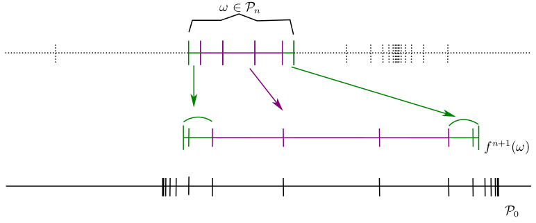
  Figure 5. Illustration of the refinement of $\omega\in{\mathcal{P}}_{n}$.

  This family $\bar{\mathcal{Q}}=\{\bar{\eta}_{c,p}\}$ is a partition of $\omega$ Lebesgue modulo zero such that $f^{n+1}(\bar{\eta}_{c,p})$ is either equal to $M(c,p)$; or strictly contained in $M(c,p)$.

  In the latter case, $f^{n+1}(\bar{\eta}_{c,p})$ is necessarily at an extreme of the interval $f^{n+1}(\omega)$ and we join $\bar{\eta}_{c,p}$ with its neighbor in ${\mathcal{Q}}$ obtaining an interval $\eta_{c,p}$.

  In this way we construct a new partition ${\mathcal{Q}}=\{\eta_{c,p}\}$ of $\omega$ which satisfies

  $$M(c,p)\subseteq f^{n+1}(\eta_{c,p})\subseteq M(c,p)^{+};$$ (4.18)

  for all $(c,p)$ with either $c\in{\mathcal{S}}$ and $p\geq\rho(c)$, or $c\in{\mathcal{D}}\setminus{\mathcal{S}}$ and $p\geq\rho_{0}-1$, so that $\eta_{c,p}\in{\mathcal{Q}}$; and we set

  $$\eta_{c,p}\in{\mathcal{P}}_{n+1},\quad R_{n+1}(\eta_{c,p}) =R_{n}(\eta_{c,p})\cup\{n+1\}\quad\text{and}\quad$$

  $$D_{n+1}(\eta_{c,p}) =D_{n}(\eta_{c,p})\cup\{(c,p)\}.$$

  The cases $\eta_{c,\rho_{0}-1}\in{\mathcal{Q}}$ with $c\in{\mathcal{D}}\setminus{\mathcal{S}}$ are a special kind of return time, identified in what follows by naming $n+1$ an escape time for the points of $\eta_{c,\rho_{0}-1}$.

Remark 4.4.

If $\eta_{c,\rho_{0}}\in{\mathcal{Q}}$, then we might have $M(c,\rho_{0}-1)\cap f^{n+1}\eta_{c,\rho_{0}}\neq\emptyset$ but even in this case $M(c,\rho_{0}-1)$ is not necessarily covered; see Figure 6.

To finish the refining algorithm, we repeat the procedure for each $\omega\in{\mathcal{P}}_{n}$ completing the construction of ${\mathcal{P}}_{n+1}$ from ${\mathcal{P}}_{n}$ for $n\geq 1$.

Clearly, since the atoms of the initial partition ${\mathcal{P}}_{0}$ are intervals, then this construction shows that all the atoms of ${\mathcal{P}}_{n}$ are intervals, for all $n\geq 1$.

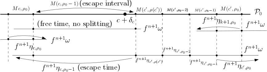
Figure 6. Illustration of different relative positions of $f^{n+1}\omega$ and atoms of ${\mathcal{P}}_{0}$ between consecutive elements of $c\in{\mathcal{D}}\setminus{\mathcal{S}}$ and $c^{\prime}\in{\mathcal{S}}$. Note how enforcing splitting of $f^{n+1}\omega$ only if it intersects more than $3$ elements of ${\mathcal{P}}_{0}$ ensures that a certain proportion of $\omega$ is removed to obtain any $\eta_{c,p}$.

4.3. Measure of atoms of ${\mathcal{P}}_{n}$ as a function of return depths

Here we estimate the measure of $\omega\in{\mathcal{P}}_{n}$ using $R_{n}(\omega)$ and $D_{n}(\omega)$ in a similar way to [7, Section 6.4] but with the new length/distance relations from (4.9).

We start by fixing $n\in{\mathbb{Z}}^{+}$, $u\in\{1,\dots,n\}$ and taking $\omega^{0}\in{\mathcal{P}}_{0}$. Let $\omega\in{\mathcal{P}}_{n}$ be such that $\omega\subset\omega^{0}$ and $u_{n}(\omega)=u=\#\mathcal{R}_{n}(\omega)$ is the number of return times $R_{n}(\omega)=\{t_{0},t_{1},\dots,t_{u}\}$ of $\omega$, where $0=t_{0}<t_{1}<\dots<t_{u}\leq n$; and $D_{n}(\omega)=\{(c_{1},p_{1}),\dots,(c_{u},p_{u})\}$ be the return depths determined by $\omega$ through the refinement algorithm.

For $m=1,\dots,u$ we write $\omega^{m}=\omega((c_{1},p_{1}),\dots,(c_{m},p_{m}))\in{\mathcal{P}}_{t_{m}}$ the subset of $\omega^{0}$ satisfying

$$f^{t_{i}}(\omega^{m})\subset M(c_{i},p_{i})^{+},1\leq i<m\,\mbox{ and }\,M(c_{m},p_{m})\subset f^{t_{m}}(\omega^{m})\subset M(c_{m},p_{m})^{+},$$ (4.19)

by the definition of the sequence of partitions ${\mathcal{P}}_{n}$. We get a nested sequence of sets

$$\omega^{0}\supsetneq\omega^{1}\supsetneq\dots\supsetneq\omega^{u}=\omega.$$

Fixing $u\leq n$ and $p_{1},\dots,p_{u}$, we define

$${\mathcal{T}}=\{\omega\in{\mathcal{P}}_{n}:\omega\subset\omega^{0},\,u_{n}(\omega)=u\quad\text{and}\quad D_{n}(\omega)=\{(c_{1},p_{1}),\dots,(c_{u},p_{u})\},c_{i}\in{\mathcal{D}}\},$$

this is, the set of points contained in atoms of ${\mathcal{P}}_{n}$ which lie inside $\omega^{0}$ and whose first $n$ iterates have a given number $u$ of return times and a given sequence $p_{1},\dots,p_{u}$ of return depths.

Now we define by induction a sequence of refinements of ${\mathcal{T}}$ which will enable us to determine the estimates we need. Start by putting ${\mathcal{V}}_{0}=\omega^{0}$. We define for $1\leq i\leq u$

$${\mathcal{V}}_{i}=\bigcup\{\omega^{i}:\omega\in{\mathcal{T}}\,\&\,\eqref{eq:nested}\text{ holds with }m=i\}$$

and note that ${\mathcal{V}}_{i}\subset{\mathcal{V}}_{i-1}$. Next we compare $\big{|}{\mathcal{V}}_{j}\big{|}$ with $\big{|}{\mathcal{V}}_{j-1}\big{|},j=1,\dots,u$, using the conditions on $\rho_{0}$ and definitions of $\beta_{2},\beta_{3},\underline{\beta}$ given in Subsection 4.2.2.

Lemma 4.5.

There exists $\zeta_{0}=\zeta_{0}(\rho_{0})>0$ such that

$$\big{|}{\mathcal{V}}_{m}\big{|} \leq e^{-\zeta_{0}}\big{|}{\mathcal{V}}_{m-1}\big{|},\quad m=1,\dots,u.$$ (4.20)

Moreover, if $p_{m}>\rho_{0}$ for any $m\in\{1,\dots,u\}$, then

$$\big{|}{\mathcal{V}}_{m}\big{|} \leq\frac{1}{L^{2}\kappa_{0}\sigma^{t_{m}-t_{m-1}-1}}\cdot\frac{|M(c_{m},p_{m})|^{\beta_{3}}}{|M(c_{m-1},p_{m-1})|^{\beta_{2}}}|{\mathcal{V}}_{m-1}|.$$ (4.21)

These estimates provide the general bound

$$|{\mathcal{V}}_{u}|\leq|\omega^{0}|^{1-\beta_{2}}e^{-\zeta_{0}(n-R)}\sigma^{-R+r}\prod_{p_{i}>\rho_{0}}|M(c_{i},p_{i})|^{\beta_{3}-\beta_{2}},$$ (4.22)

where $R$ is the number of iterates between the $r$ return times having depth larger than $\rho_{0}$.

Assuming the lemma, we fix $n\geq 1$, the escape/return times $0=t_{0}<t_{1}<\dots<t_{u}\leq n$ and $(c_{1},p_{1}),\dots,(c_{u},p_{u})$ and consider the subset

$$A^{u} =A^{u}_{(c_{1},p_{1}),\dots,(c_{u},p_{u})}(n)=\big{\{}x\in M:u_{n}(x)=u\text{ and }f^{t_{i}}(x)\in M(c_{i},p_{i}),\,i=1,\dots,u\big{\}}$$

$$=\big{\{}x\in\omega\in{\mathcal{P}}_{n}:D_{n}(\omega)=\{(c_{0},p_{0}),(c_{1},p_{1}),\dots,(c_{u},p_{u})\}\big{\}}$$

where $c_{i}\in{\mathcal{D}},p_{i}\geq\rho_{0}-1,i=0,1,\dots,u$ and $u_{n}(x)$ for $x\in\omega\in{\mathcal{P}}_{n}$ denotes the number of escape/returns of $\omega$ until the $n$th iterate. Then from (4.22) we get

$$|A^{u}_{(c_{1},p_{1}),\dots,(c_{u},p_{u})}(n)| \leq\sum_{\omega\in{\mathcal{P}}_{n}\cap A^{u}\atop\omega\subset\omega^{0}\in{\mathcal{P}}_{0}}e^{-\zeta_{0}(n-R)}\sigma^{-R+r}\prod_{p_{i}>\rho_{0}}|M(c_{i},p_{i})|^{\beta_{3}-\beta_{2}}\cdot|M(c_{0},p_{0})|^{1-\beta_{2}}$$

$$\leq e^{-\zeta_{0}(n-R)}\sigma^{-R+r}\prod_{p_{i}>\rho_{0}}|M(c_{i},p_{i})|^{\beta_{3}-\beta_{2}}\sum_{\omega_{0}\in{\mathcal{P}}_{0}}|\omega^{0}|^{1-\beta_{2}}$$

$$\leq C_{0}e^{-\zeta_{0}(n-R)}\sigma^{-R+r}\prod_{p_{i}>\rho_{0}}|M(c_{i},p_{i})|^{\beta_{3}-\beta_{2}},$$ (4.23)

where $C_{0}=\sum_{\omega_{0}\in{\mathcal{P}}_{0}}|\omega^{0}|^{1-\beta_{2}}>1$ depends only on $\beta_{1}$ and $\varepsilon_{1}$. This is well-defined since $1-\beta_{1}>\varepsilon_{1}\beta_{1}$, by the choice of $\varepsilon_{1}$, and denoting $\#{\mathcal{D}}$ the number of elements of ${\mathcal{D}}$:

$$C_{0}\leq\#{\mathcal{D}}\cdot\sum_{p\geq\rho_{0}}\big{(}p^{-1-1/(\varepsilon_{1}\beta_{1})}\big{)}^{(1-\beta_{1})(1+\varepsilon_{1}\beta_{1})}=\#{\mathcal{D}}\sum_{p\geq\rho_{0}}p^{-\frac{1-\beta_{1}}{\varepsilon_{1}\beta_{1}}}<\infty.$$

The proof of Lemma 4.5 is contained in the remaining of this subsection.

4.3.1. Between return times not considering relative depths

Now we start the proof of Lemma 4.5. Let us assume that $m\in\{1,\dots,u\}$ and $t_{m}$ is an escape time: $p_{m}=\rho_{0}-1$ and $c_{m}\in{\mathcal{D}}\setminus{\mathcal{S}}$. Then by the partition algorithm, bounded distortion and (4.5) (recall Figure 6)

$$\frac{|\omega^{m-1}\setminus\omega^{m}|}{|\omega^{m-1}|} \geq\frac{1}{D^{2}}\cdot\frac{|f^{t_{m}}(\omega^{m-1}\setminus\omega^{m})|}{|f^{t_{m}}\omega^{m-1}|}\geq\frac{1}{D^{2}}\cdot\frac{|M(c,p)|}{|M(c_{m},\rho_{0}-1)^{+}|}$$

where $M(c,p)$ is one of the neighbors of $M(c_{m},\rho_{0}-1)$ in ${\mathcal{P}}_{0}$: either $M(c_{m},\rho_{0})$; or $M(c,\rho_{0})$ for some $c\in{\mathcal{D}}\setminus{\mathcal{S}},c\neq c_{m}$; or else $c\in{\mathcal{S}}$ and $p=\rho(c)\leq\rho_{0}-1$.

If $t_{m}$ is such that $p_{m}=\rho_{0}$ and $c_{m}\in{\mathcal{D}}\setminus{\mathcal{S}}$, then analogously we obtain

$$\frac{|\omega^{m-1}\setminus\omega^{m}|}{|\omega^{m-1}|} \geq\frac{1}{D^{2}}\cdot\frac{|M(c_{m},\rho_{0}+1)|}{|M(c_{m},\rho_{0})^{+}|}.$$

Otherwise, either $p_{m}<\rho_{0}$ and then $c_{m}\in{\mathcal{S}}$; or $p_{m}>\rho_{0}$ and we similarly obtain

$$\frac{|\omega^{m-1}\setminus\omega^{m}|}{|\omega^{m-1}|} \geq\frac{1}{D^{2}}\cdot\frac{|M(c_{m},p)|}{|M(c_{m},p_{m})^{+}|}>\frac{1}{K_{1}D^{2}},$$

where $M(c_{m},p)$ is one of the neighbors of $M(c_{m},p_{m})$ in ${\mathcal{P}}_{0}$ in the one-sided neighborhood of $c_{m}$. So in all cases $\frac{|\omega^{m-1}\setminus\omega^{m}|}{|\omega^{m-1}|}\geq\frac{\xi(\rho_{0})}{D^{2}},$ where $\xi(\rho_{0})=\frac{1}{K_{0}K_{1}}\inf_{c\in{\mathcal{D}}\setminus{\mathcal{S}}}\frac{(\rho_{0}+1)^{-1-\varepsilon_{1}\beta_{1}}}{2\delta_{c}-(\rho_{0}+2)^{-1/(\varepsilon_{1}\beta_{1})}}$.

This proves (4.20) since

$$|{\mathcal{V}}_{m}| =\sum_{\omega^{m}\in{\mathcal{V}}_{m}}|\omega^{m}|=\sum_{\omega^{m}\in{\mathcal{V}}_{m}\atop\omega^{m}\subset\omega^{m-1}\in{\mathcal{V}}_{m-1}}\frac{\big{|}\omega^{m-1}\setminus(\omega^{m-1}\setminus\omega^{m})\big{|}}{|\omega^{m-1}|}|\omega^{m-1}|$$

$$\leq\left(1-\frac{\xi}{D^{2}}\right)\sum_{\omega^{m}\subset\omega^{m-1}\in{\mathcal{V}}_{m-1}}|\omega^{m-1}|\leq e^{-\zeta_{0}}|{\mathcal{V}}_{m-1}|,\text{ for }0<\zeta_{0}<\zeta=-\log(1-\xi/D^{2}).$$

Remark 4.6.

1. Note that $\zeta=\zeta(\rho_{0})\xrightarrow[\rho_{0}\nearrow\infty]{}0$. Moreover, the estimates in this subsection depend on the requirement in the refining algorithm of only splitting the intervals when they intersect more than three elements of ${\mathcal{P}}_{0}$.

2. Since $1\geq|f^{t_{m}}\omega^{m-1}|\geq\sigma^{t_{m}-t_{m-1}}|f^{t_{m-1}}\omega^{m-1}|\geq\sigma^{t_{m}-t_{m-1}}|M(c_{m-1},p_{m-1})|$ we deduce $t_{m}-t_{m-1}\leq-\log|M(c_{m-1},p_{m-1})|/\log\sigma$. Hence the number of iterates between consecutive return times is bounded by the depth of the first return.

3. In particular, if $t_{m-1}$ is an escape time, i.e. $p_{m-1}=\rho_{0}-1$ and $c_{m-1}\in{\mathcal{D}}\setminus{\mathcal{S}}$, then $t_{m}-t_{m-1}\leq L_{0}$ for a uniform constant $L_{0}$ depending only on the minimum length of $M(c,\rho_{0}-1)$ for $c\in{\mathcal{D}}\setminus{\mathcal{S}}$. Because $|M(c,\rho_{0}-1)|$ grows to $\delta_{c}$ as $\rho_{0}\nearrow\infty$, then this shows that the number of iterates between consecutive escape times is uniformly bounded by a constant which does not depend on $\rho_{0}$.

4.3.2. Between returns which are not escape times

We fix $m\in\{1,\dots,u\}$. On the one hand, note that if $p_{m-1}\geq\rho_{0}$, then by the partition algorithm, either $c=c_{m-1}\in{\mathcal{S}}$ and we get the bound

$$\frac{\big{|}\omega^{m}\big{|}}{\big{|}\omega^{m-1}\big{|}} \leq\frac{\big{|}\omega^{m}\big{|}}{\big{|}\widehat{\omega}^{m-1}\big{|}}\leq D^{2}\cdot\frac{\Big{|}f^{t_{m}}\omega^{m}\Big{|}}{\Big{|}f^{t_{m}}\widehat{\omega}^{m-1}\Big{|}},\text{ where }\widehat{\omega}^{m-1}=\omega^{m-1}\cap f^{-t_{m}}({\mathcal{U}}_{0})$$

$$\leq D^{2}\cdot\frac{\big{|}M(c_{m},p_{m})^{+}\big{|}}{\sigma^{t_{m}-t_{m-1}-1}|f^{\prime}(\xi)|\cdot\big{|}f^{t_{m-1}}\widehat{\omega}^{m-1}\big{|}}\text{ for some }\xi\in f^{t_{m-1}}\widehat{\omega}^{m-1};$$ (4.24)

or $c=c_{m-1}\in{\mathcal{D}}\setminus{\mathcal{S}}$ and we use (4.1)

$$\Big{|}f^{t_{m}}\widehat{\omega}^{m-1}\Big{|}\geq\sigma^{t_{m}-t_{m-1}-T(c)-1}|f^{\prime}(\zeta)|\cdot\big{|}f^{t_{m-1}+T(c)}\widehat{\omega}^{m-1}\big{|}\geq\sigma^{t_{m}-t_{m-1}-1}|f^{\prime}(\zeta)|\cdot\big{|}f^{t_{m-1}}\widehat{\omega}^{m-1}\big{|}$$

for some $\zeta\in f^{t_{m-1}+T(c)}\widehat{\omega}^{m-1}$; where $\widehat{\omega}^{m-1}$ restricts focus in the denominator to points which lie in the return region ${\mathcal{U}}_{0}=\cup_{c\in{\mathcal{D}}}\cup_{p\geq\rho_{0}-1}I(c,p)$ whose trajectories are controlled by the refinement algorithm.

If $c\in{\mathcal{S}}$, by Lemma 4.1 and the choice of $\widehat{\omega}^{m-1}$

$$|f^{\prime}(\xi)|\geq\frac{\left(p_{m-1}^{\gamma}\right)^{\beta_{1}-1}}{B}=\frac{p_{m-1}^{(1-\beta_{1})/\varepsilon_{1}\beta_{1}}}{B}>\frac{K_{0}^{(\beta_{1}-1)/(1+\varepsilon_{1}\beta_{1})}}{B}|M(c,p_{m-1})|^{(\beta_{1}-1)/(1+\varepsilon_{1}\beta_{1})}$$ (4.25)

where $M(c,p_{m-1})\subset f^{t_{m-1}}\widehat{\omega}^{m-1}\subset f^{t_{m-1}}\omega^{m-1}$ by definition of return time. Otherwise, $c\in{\mathcal{D}}\setminus{\mathcal{S}}$ and by the previous estimates together with (4.7), noting that $(\beta_{1}-1)/(1+\varepsilon_{1}\beta_{1})=\beta_{2}-1$

$$|f^{\prime}(\zeta)| \geq\frac{\left(p_{m-1}^{\gamma}\right)^{\beta_{1}-1}}{B}\geq\frac{K_{0}^{\beta_{2}-1}}{B}|M(\tilde{c},p_{m-1})|^{\beta_{2}-1}$$

$$=\frac{K_{0}^{\beta_{2}-1}}{B}|f^{T}M(c,p_{m-1})|^{\beta_{2}-1}\geq\frac{(K_{0}K_{1})^{\beta_{2}-1}}{B}|M(c,p_{m-1})|^{\beta_{2}-1}$$ (4.26)

where $\tilde{c}=f^{T}c$ is the singularity to which $c$ is connected.

On the other hand, if $p_{m-1}=\rho_{0}-1$ and $c\in{\mathcal{D}}\setminus{\mathcal{S}}$, then we use the conditions from Subsection 4.2.2 to deduce

$$|f^{t_{m-1}+1}\omega^{m-1}|\geq\sigma|M(c,\rho_{0}-1)|\geq|M(c,\rho_{0}-1))|^{\underline{\beta}}.$$ (4.27)

Since $K_{1}>K_{0}>1$, in any of the cases above we arrive at

$$\frac{\big{|}\omega^{m}\big{|}}{\big{|}\omega^{m-1}\big{|}} \leq\frac{BD^{2}(K_{1}K_{0})^{\beta_{2}-1}}{\sigma^{t_{m}-t_{m-1}-1}}\cdot\frac{\big{|}M(c_{m},p_{m})^{+}\big{|}}{|M(c_{m-1},p_{m-1})|^{\max\{\beta_{2},\underline{\beta}\}}}.$$ (4.28)

Now if $t_{m}$ is such that $p_{m}>\rho_{0}$, then from (4.16) we can bound (4.28) as

$$\frac{L|M(c_{m},p_{m})^{+}|}{\kappa_{0}\sigma^{\Delta t_{m}-1}|M(c_{m},p_{m})|^{\beta_{3}}}\cdot\frac{|M(c_{m},p_{m})|^{\beta_{3}}}{|M(c_{m-1},p_{m-1})|^{\beta_{2}}}\leq\frac{1}{L^{2}\kappa_{0}\sigma^{\Delta t_{m}-1}}\cdot\frac{|M(c_{m},p_{m})|^{\beta_{3}}}{|M(c_{m-1},p_{m-1})|^{\beta_{2}}},$$

where $\Delta t_{m}=t_{m}-t_{m-1}$. Now we can obtain (4.21)

$$|{\mathcal{V}}_{m}| =\sum_{\omega^{m}\in{\mathcal{V}}_{m}}|\omega^{m}|=\sum_{\omega^{m}\in{\mathcal{V}}_{m}\atop\omega^{m}\subset\omega^{m-1}\in{\mathcal{V}}_{m-1}}\frac{|\omega^{m}|}{|\omega^{m-1}|}|\omega^{m-1}|\leq\frac{1}{L^{2}\kappa_{0}\sigma^{\Delta t_{m}-1}}\cdot\frac{|M(c_{m},p_{m})|^{\beta_{3}}}{|M(c_{m-1},p_{m-1})|^{\beta_{2}}}|{\mathcal{V}}_{m-1}|.$$

This completes the proof of all but the last estimate in Lemma 4.5.

4.3.3. Probability of a given sequence of returns

Now we apply the estimates (4.20) and (4.21) to prove (4.22). Consider $s_{0}=0<1\leq r_{1}<s_{1}<r_{2}<s_{2}<\dots<r_{h}<s_{h}\leq u<r_{h+1}=u+1$ the indexes marking the beginning of sequences of return times with return depths $p\leq\rho_{0}$ from $t_{s_{i}}$ to $t_{r_{i+1}-1}$ within $t_{1}<t_{2}<\dots<t_{u}$; and sequences of consecutive return times with depth $p>\rho$ from $t_{s_{i}}$ to $t_{r_{i+1}-1}$.

More precisely, for each $j=0,\dots,h$ we have for $r_{j}\leq i<s_{j}$ that $p_{i}>\rho_{0}$; and for $s_{j}\leq i<r_{j+1}$ we have $p_{i}\leq\rho_{0}$. Using this grouping of the consecutive return times we obtain that

• every pair of return times with depth $p\leq\rho_{0}$ introduces a factor $e^{-\zeta}$ as in (4.20);

• the remaining pairs of return times introduce quotients as in (4.21).

Now the details: assuming first that $r_{1}=1$ and $s_{h}=u$, then $|{\mathcal{V}}_{u}|=|{\mathcal{V}}_{0}|\prod_{i=1}^{u}\frac{|{\mathcal{V}}_{i}|}{|{\mathcal{V}}_{i-1}|}$ and we can group the iterates from $s_{0}=0=r_{1}-1$ to $s_{1}-1$, the transition to $s_{1}$ together with the iterates from $s_{1}$ to $r_{2}-1$

$$|{\mathcal{V}}_{r_{2}-1}| =|{\mathcal{V}}_{0}|\prod_{i=r_{1}}^{r_{2}-1}\frac{|{\mathcal{V}}^{i}|}{|{\mathcal{V}}^{i-1}|}\leq e^{-\zeta(r_{2}-s_{1})}|\omega^{0}||M(c_{s_{1}-1},p_{s_{1}-1})|^{\beta_{3}}\prod_{j=r_{1}}^{s_{1}-2}\frac{|M(c_{j},p_{j})|^{\beta_{3}}}{L^{2}\kappa_{0}\sigma^{\Delta t_{j}-1}|M(c_{j-1},p_{j-1})|^{\beta_{2}}}$$

$$\leq e^{-\zeta(r_{2}-s_{1})}|\omega_{0}|^{1-\beta_{2}}\frac{|M(c_{s_{1}-1},p_{s_{1}-1})|^{\beta_{3}}}{(L^{2}\kappa_{0})^{s_{1}-r_{1}-1}}\prod_{j=1}^{s_{1}-2}\frac{|M(c_{j},p_{j})|^{\beta_{3}-\beta_{2}}}{\sigma^{\Delta t_{j}-1}}.$$

Repeating for the groups of iterates from $s_{j}$ to $s_{j+1}-1$ and including the transition from $s_{j}-1$ to $s_{j}$, for $j=1,\dots,h$, we obtain, writing $s=\sum_{j=1}^{h}(r_{j}-s_{j-1})$ for the number returns in a chain of return times with $p_{i}\leq\rho_{0}$, and using (4.17)

$$|{\mathcal{V}}_{u-1}| \leq\frac{e^{-\zeta s}}{|\omega^{0}|^{\beta_{2}-1}}\prod_{j=1}^{h}\frac{|M(c_{s_{h}-1},p_{s_{h}-1})|^{\beta_{3}}}{(L^{2}\kappa_{0})^{s_{j}-r_{j}-1}|M(c_{r_{j+1}-1},\rho_{0}-1)|^{\beta_{2}}}\prod_{r_{j}\leq i<s_{j}-1}\frac{|M(c_{i},p_{i})|^{\beta_{3}-\beta_{2}}}{\sigma^{\Delta t_{i}-1}}$$

$$\leq e^{-\zeta s}|\omega^{0}|^{1-\beta_{2}}\prod_{j=1}^{h}\frac{1}{(L^{2}\kappa_{0})^{s_{j}-r_{j}-1}}\prod_{r_{j}\leq i<s_{j}}\frac{|M(c_{i},p_{i})|^{\beta_{3}-\beta_{2}}}{\sigma^{\Delta t_{i}-1}}.$$

Now since $s_{h}=u$, by (4.28) the definition of $\kappa_{0}$ and the choice of $\rho_{0}$, we get

$$|{\mathcal{V}}_{u}| =\frac{|{\mathcal{V}}_{u}|}{|{\mathcal{V}}_{u-1}|}|{\mathcal{V}}_{u-1}|\leq\frac{L}{\kappa_{0}\sigma^{\Delta t_{u}}}\cdot\frac{|M(c_{u},\rho_{0}-1)^{+}|}{|M(c_{u-1},p_{u-1})|^{\beta_{2}}}\cdot|{\mathcal{V}}_{u-1}|$$

$$\leq|M(c_{u},\rho_{0}-1)|^{\beta_{2}}\frac{e^{-\zeta s}|\omega^{0}|^{1-\beta_{2}}}{\sigma^{\Delta t_{u}}}\prod_{j=1}^{h}\prod_{r_{j}\leq i<s_{j}-1}\frac{|M(c_{i},p_{i})|^{\beta_{3}-\beta_{2}}}{\sigma^{\Delta t_{i}-1}}.$$ (4.29)

Moreover, because $s_{h}=u$, then $f^{t_{u}}\omega^{u}\supset M(c_{u},\rho_{0}-1)$ and $f^{t_{u}+j}\omega^{u}$ has no returns for $j=1,\dots,n-t_{u}$. Thus by (4.27)

$$1 \geq|f^{n}\omega^{u}|=|f^{n-t_{u}-1}(f^{t_{u}+1}\omega^{u})|\geq\sigma^{n-t_{u}-1}|f^{t_{u}}\omega^{u}|^{\underline{\beta}}$$

and then $|M(c_{u},\rho_{0}-1)|^{\beta_{2}}\leq|f^{t_{u}}\omega^{u}|^{\beta_{2}}\leq|f^{t_{u}}\omega^{u}|^{\underline{\beta}}\leq\sigma^{t_{u}-n+1}$. Writing

• $R=\sum_{j=1}^{h}(t_{s_{j}+1}-t_{r_{j}})$ for the quantity of iterations between return times with depth $p>\rho_{0}$ from the $r_{j}$-th to $(s_{j}+1)$-th return, and

• $r=\sum_{j=1}^{h}(s_{j}-r_{j})$ for the quantity of return times involved in this chain of returns;

we arrive at

$$\big{|}{\mathcal{V}}_{u}\big{|} \leq|\omega^{0}|^{1-\beta_{2}}e^{-\zeta s}\sigma^{t_{u}-n+1-R+r}\prod_{p_{i}>\rho_{0}}|M(c_{i},p_{i})|^{\beta_{3}-\beta_{2}}.$$ (4.30)

Now we use the last expression to obtain the other cases: we might have $1<r_{1}$ or $s_{h}<u$, and so there is an initial and/or final sequence of consecutive escape times. Since

$$|{\mathcal{V}}_{u}| =|{\mathcal{V}}_{0}|\prod_{i=1}^{r_{1}-1}\frac{|{\mathcal{V}}_{i}|}{|{\mathcal{V}}_{i-1}|}\prod_{i=r_{1}}^{s_{h}}\frac{|{\mathcal{V}}_{i}|}{|{\mathcal{V}}_{i-1}|}\prod_{i=s_{h}+1}^{u}\frac{|{\mathcal{V}}_{i}|}{|{\mathcal{V}}_{i-1}|}$$

we can bound the middle product by the expression (4.29) with $M(c_{r_{1}-1},\rho_{0}-1)$ in the place of $\omega^{0}$ and $s_{h}$ in the place of $u$:

$$\prod_{i=r_{1}}^{s_{h}}\frac{|{\mathcal{V}}_{i}|}{|{\mathcal{V}}_{i-1}|} \leq\frac{e^{-\zeta s}L|M(c_{s_{h}},\rho_{0}-1)^{+}|}{\kappa_{0}\sigma^{\Delta t_{s_{h}}}|M(c_{r_{1}-1},\rho_{0}-1)|^{\beta_{2}}}\prod_{j=1}^{h}\prod_{r_{j}\leq i<s_{j}}\frac{|M(c_{i},p_{i})|^{\beta_{3}-\beta_{2}}}{\sigma^{\Delta t_{i}-1}}$$

$$\leq e^{-\zeta s}\sigma^{-R+r}\prod_{p_{i}>\rho_{0}}|M(c_{i},p_{i})|^{\beta_{3}-\beta_{2}},$$

where $s=\sum_{j=2}^{h}(r_{j}-s_{j-1})$. Finally, the first factor is bounded according to Subsection 4.3.1

$$|{\mathcal{V}}_{0}|\prod_{i=1}^{r_{1}-1}\frac{|{\mathcal{V}}_{i}|}{|{\mathcal{V}}_{i-1}|}\leq e^{-\zeta(r_{1}-2)}|{\mathcal{V}}_{1}|\leq e^{-\zeta(r_{1}-2)}|\omega^{0}|=e^{-\zeta(r_{1}-s_{0}-2)}|\omega^{0}|$$

and likewise the last factor is bounded by $e^{-\zeta(u-s_{h}-1)}=e^{-\zeta(r_{h+1}-s_{h}-2)}$. Hence writing $\bar{s}=s+r_{h+1}-s_{h}-1+r_{1}-s_{0}-1$ to incorporate all the return times inside all chains of returns with depth at most $\rho_{0}$, we arrive at

$$|{\mathcal{V}}_{u}|\leq|\omega^{0}|^{1-\beta_{2}}e^{-\zeta\bar{s}}\sigma^{-R+r}\prod_{p_{i}>\rho_{0}}|M(c_{i},p_{i})|^{\beta_{3}-\beta_{2}}.$$

In addition, by Remark 4.6(3) the total number of iterates between consecutive escape times is related to the number of escapes times by $\bar{s}L_{0}\geq\sum_{j=0}^{h}(t_{r_{j+1}}-t_{s_{j}+1})=n-R,$ so $e^{-\zeta\bar{s}}\leq e^{-\frac{\zeta}{L_{0}}(n-R)}$. Hence $|{\mathcal{V}}_{u}|\leq|\omega^{0}|^{1-\beta_{2}}e^{-\frac{\zeta}{L_{0}}(n-R)}\sigma^{-R+r}\prod_{p_{i}>\rho_{0}}|M(c_{i},p_{i})|^{\beta_{3}-\beta_{2}}.$ This provides the general bound (4.22) after setting $\zeta_{0}=\zeta/L_{0}$ and completes the proof of Lemma 4.5.

4.4. Distance to the singular set between returns

We show that the distance to the singular set for iterates $t_{i}<j<t_{i+1}$ between return times of a given $\omega\in{\mathcal{P}}_{n}$ is controlled by the depth of the last return time, as follows.

In the same setting since the beginning of this section, by the refinement algorithm we can write $M(c_{i},p_{i})\subset f^{t_{i}}\omega^{i}\subset M(c_{i},p_{i})^{+}$, where either $c_{i}\in{\mathcal{S}}$ and $p_{i}\geq\rho(c)$, or $c_{i}\in{\mathcal{D}}\setminus{\mathcal{S}}$ and $p_{i}\geq\rho_{0}-1$, since $t_{i}$ is a return.

We also have that there are $(c^{j},p^{j})$ so that $f^{j}\omega^{i}\subset f^{j}M(c_{i},p_{i})^{+}\subset M(c^{j},p^{j})^{+}$, where $p^{j}\geq\rho(c^{j})$ for $c^{j}\in{\mathcal{S}}$ or $p^{j}\geq\rho_{0}-1$ for $c^{j}\in{\mathcal{D}}\setminus{\mathcal{S}}$; and $f^{j}\mid\omega^{i}:\omega^{i}\to f^{j}\omega^{i}$ is a diffeomorphism, for each $j=t_{i}+1,\dots,t_{i+1}-1$. These are the host intervals at iterate $t_{i}<j<t_{i+1}$.

Remark 4.7.

These intervals are well-defined since the refinement algorithm only splits $f^{j}\omega^{i}$ when this interval intersects more that $3$ intervals of ${\mathcal{P}}_{0}$.

Moreover, we can compare the distance to the singular set with the length of the host interval following (4.9) and noting that $d(M(c,\rho_{0}-1)^{+},{\mathcal{D}})=d(M(c,\rho(c)),{\mathcal{D}})$. In addition, from (4.15), we assume that

$$2\delta<\inf\{\bar{\delta},\operatorname{dist}(M(c,\rho_{0}-1)^{+},{\mathcal{D}}):c\in{\mathcal{D}}\setminus{\mathcal{S}}\}$$ (4.31)

in what follows. Next we divide the iterates $j=t_{i},\dots,t_{i+1}-1$ into sequences of consecutive visits near a singularity and connection iterates between a discontinuity and a singularity.

If $c_{i}\in{\mathcal{D}}\setminus{\mathcal{S}}$ with $p_{i}>\rho_{0}$, then $\operatorname{dist}_{\delta}(f^{j}\omega^{i},{\mathcal{D}})=1$ for $t_{i}<j<t_{i}+T,T=T(c_{i})$ by the choice of $\delta$. By construction of the partition $f^{t_{i}+T}(\omega^{i})\supset M(\tilde{c}_{i},p)$ for some $\tilde{c}_{i}\in{\mathcal{S}}$ and so $|f^{t_{i}+T}(\omega^{i})|\geq\sigma^{T}|f^{t_{i}}\omega^{i}|>|M(c_{i},p_{i})|$ which implies from (4.9) that $\sum_{j=t_{i}}^{t_{i}+T-1}\log\operatorname{dist}_{\delta}(f^{j}\omega^{i},{\mathcal{D}})$ equals

$$\log\operatorname{dist}_{\delta}(f^{t_{i}}\omega^{i},{\mathcal{D}})\geq\log\frac{|M(c_{i},p_{i})|^{\frac{1}{1+\varepsilon_{1}\beta_{1}}}}{K_{2}}\geq\log|M(c_{i},p_{i})|.$$ (4.32)

Remark 4.8.

We can assume without loss of generality that $p_{i}>\rho_{0}$ for $c_{i}\in{\mathcal{D}}\setminus{\mathcal{S}}$. Otherwise we have $M(c_{i},p_{i})\subset f^{t_{i}}\omega^{i}$ and consequently $f^{j}M(c_{i},p_{i})\subset f^{t_{i}+j}\omega^{i}\subset M(c^{j},p^{j})^{+}$ with $p_{i}=\rho_{0}$ or $p_{i}=\rho_{0}-1$, which implies that $|M(c^{j},p^{j})^{+}|\geq\sigma^{j}|M(c_{i},p_{i})|$ and so $p^{j}\leq\rho_{0}$ for all $0<j<t_{i+1}$. Hence $f^{j}\omega^{i}$ is $2\delta$-away from ${\mathcal{D}}$ by the choice of $\delta$, so all the iterates $t_{i}\leq j<t_{i+1}$ are truncated: $\sum_{j=t_{i}}^{t_{i+1}-1}-\log\operatorname{dist}_{\delta}(f^{j}\omega^{i},{\mathcal{D}})=0$.

By the Mean Value Theorem and (4.1) we get

$$\frac{|f^{j+1}\omega^{i}|}{|f^{j}\omega^{i}|}=|f^{\prime}(\xi_{j})|\geq\frac{d(\xi_{j},c^{j})^{\beta_{1}-1}}{B},\quad\text{for some}\quad\xi_{j}\in f^{j}\omega^{i}\quad\text{if $c^{j}\in{\mathcal{S}}$}.$$

If $(c^{j},p^{j})$ has $c^{j}\in{\mathcal{S}}$, then from (4.5),  (4.9) and (4.17) the quotient $\frac{|f^{j+1}\omega^{i}|}{|f^{j}\omega^{i}|}$ is bigger than

$$\frac{d(M(c^{j},p^{j})^{+},c^{j})^{\beta_{1}-1}}{B}\geq\frac{|M(c^{j},p^{j}+1)|^{\frac{\beta_{1}-1}{1+\varepsilon_{1}\beta_{1}}}}{BK_{2}^{1-\beta_{1}}}\geq\begin{cases}\frac{|M(c^{j},p^{j})|^{\beta_{3}-1}}{BK_{2}^{1-\beta_{1}}}\text{ if }\rho(c)\leq p\leq\rho_{0}\\ |M(c^{j},p^{j})|^{\beta_{3}-1}\text{ if }p>\rho_{0}\end{cases}.$$ (4.33)

In particular, for $j=t_{i}+T(a_{k_{i}})$ we necessarily have $c^{j}=\tilde{c}_{i}$ and $p^{j}=p_{i}$ by the construction of the refinement, then

$$|f^{t_{i}+T+1}\omega^{i}|\geq\frac{|M(\tilde{c}_{i},p_{i}+1)|^{\beta_{2}-1}}{BK_{2}^{1-\beta_{1}}}|f^{t_{i}+T}\omega^{i}|\geq\frac{|M(c_{i},p_{i}+1)|^{\beta_{2}-1}}{BK_{2}^{1-\beta_{1}}K_{1}^{1-\beta_{2}}}|M(\tilde{c}_{i},p_{i})|>|M(c_{i},p_{i})|^{\beta_{3}}.$$

Finally, if $c^{j}\in{\mathcal{D}}\setminus{\mathcal{S}}$ and $p^{j}>\rho_{0}$ for $j>t_{i}+T$, then from (4.15) there are no returns during times $j+1,\dots,j+T$ where $T=T(c^{j})$, hence $|f^{j+T+1}\omega^{i}|\geq\sigma^{T}|f^{j}\omega^{i}|$. Therefore, denoting by $t_{i}<\ell_{1}<\dots<\ell_{s}<t_{i+1}$ the free iterates that have an host interval near a discontinuity and $T_{m}=T(c^{\ell_{m}}),m=1,\dots,s$, we obtain the relation

$$1\geq |f^{t_{i+1}}\omega_{i}|=|f^{t_{i}+T}\omega_{i}|\prod_{j=t_{i}+T}^{\ell_{1}-1}\frac{|f^{j+1}\omega_{i}|}{|f^{j}\omega_{i}|}\left(\prod_{m=1}^{s}\prod_{j=\ell_{m}}^{\ell_{m+1}-1}\frac{|f^{j+1}\omega_{i}|}{|f^{j}\omega_{i}|}\right)\prod_{j=\ell_{s}+T_{s}}^{t_{i+1}-1}\frac{|f^{j+1}\omega_{i}|}{|f^{j}\omega_{i}|}$$

$$\geq|M(c_{i},p_{i})|^{\beta_{3}}\prod\{|M(c^{j},p^{j})|^{\beta_{3}-1}:t_{i}+T\leq j<t_{i+1},c^{j}\in{\mathcal{S}}\text{ or }j=\ell_{m},1\leq m\leq s\}.$$

Now using (4.9), (4.17) and (4.32) we get that $\sum_{j=t_{i}}^{t_{i+1}-1}\log\operatorname{dist}_{\delta}(f^{j}\omega_{i},{\mathcal{D}})$ is bounded from below by

$$\log \left(|M(c_{i},p_{i})|\prod\{|M(c^{j},p^{j})|:t_{i}+T\leq j<t_{i+1},c^{j}\in{\mathcal{S}}\text{ or }j=\ell_{m},1\leq m\leq s\}\right)$$

$$\geq\log|M(c_{i},p_{i})|+\frac{\beta_{3}}{1-\beta_{3}}\log|M(c_{i},p_{i})|=\frac{1}{1-\beta_{3}}\log|M(c_{i},p_{i})|,$$

that is

$$\sum_{j=t_{i}}^{t_{i+1}-1}-\log\operatorname{dist}_{\delta}(f^{j}\omega_{i},{\mathcal{D}})\leq\frac{1}{\beta_{3}-1}\log|M(c_{i},p_{i})|.$$ (4.34)

Finally, if $c_{i}\in{\mathcal{S}}$, then we need not use the initial sequence of $T$ iterates, so we obtain, using (4.33) perhaps with $p\leq\rho_{0}$, a similar inequality to (4.34) with a different constant.

4.4.1. Upper bound for the recurrence frequency

Consequently, we obtain the following upper bound for the recurrence frequency to ${\mathcal{D}}$ of the orbits of points of $\omega\in{\mathcal{P}}_{n}$ with given $n\geq 1$, return times $0=t_{0}<t_{1}<\dots<t_{u}\leq n$ and respective depths $(c_{1},p_{1}),\dots,(c_{u},p_{u})$

$$S_{n}\Delta_{\delta}(\omega)=\sum_{j=0}^{n-1}\Delta_{\delta}(f^{j}\omega,{\mathcal{D}}) \leq-C_{1}\sum_{j=0}^{n-1}\sum_{p_{i}>\rho_{0}}\log|M(c_{i},p_{i})|$$ (4.35)

for all $\delta$ satisfying (4.31), where $C_{1}>0$ is a constant not depending on $\omega$ or $n$ or on the return depths, not even on $\rho_{0}$ after this threshold is fixed as in Subsection 4.2.2.

4.5. Expected value of return depths and exponentially slow recurrence

Here we complete the proof of Theorem C. We estimate the expected value of deep returns up to $n$ iterates of the dynamics, proving the following statement, where we denote

$${\mathcal{D}}_{n}^{\delta}(x)=-\sum_{j=0}^{n}\sum_{i=1,\dots,u\atop p_{i}>\Theta}\log|M(c_{i},p_{i})|$$

for $\Theta\in{\mathbb{Z}}^{+}$ big enough (to be defined in the statement of Lemma 4.9 below); $\delta=\delta(\Theta)>0$ is such that

$$p>\Theta\iff d(M(c,p),{\mathcal{D}})<\delta,c\in{\mathcal{D}}\quad\text{hence}\quad\delta=\Theta^{-1/\varepsilon_{1}\beta_{1}}=a_{\Theta},$$

and $x\in\omega\in{\mathcal{P}}_{n}$ with $u=u_{n}(\omega)\leq n$ and the return depths $(c_{1},p_{1}),\dots,(c_{u},p_{u})$.

To state the result precisely, let $S(\rho,\xi)=(\#{\mathcal{D}})\cdot\sum_{p\geq\rho}|M(c_{0},p)|^{\xi}$ for any fixed $c_{0}\in{\mathcal{D}}$ and $\rho\geq\rho_{0}$. Note that this is well-defined for all $\xi>\beta_{2}+\frac{1+\varepsilon_{1}\beta_{1}}{\varepsilon_{1}\beta_{1}}$.

Lemma 4.9.

Let $\varepsilon_{0}>0$ be given and $z>0$ be such that $z<(1+\varepsilon_{1}\beta_{1})^{-1}$ and $\beta_{3}-2\beta_{2}-z>\frac{1+\varepsilon_{1}\beta_{1}}{\varepsilon_{1}\beta_{1}}$. Then for a big enough $\rho_{0}\in{\mathbb{Z}}^{+}$ satisfying all the conditions in Subsection 4.2.2 together with $S(\rho_{0},\beta_{3}-\beta_{2})<\varepsilon_{0}/2$, and for $\Theta>\rho_{0}$ such that $S(\Theta,\beta_{3}-\beta_{2}-z)<\varepsilon_{0}/2$, there exists a constant $K>0$ such that $\int_{[{\mathcal{D}}_{n}^{\delta}(x)\geq n\varepsilon/C_{1}]}e^{z{\mathcal{D}}_{n}^{\delta}(x)}\,dx\leq Ke^{\varepsilon_{0}n}$ for all $n>\varepsilon_{0}^{-1}|\log|M(c_{0},\rho_{0})||$.

This result provides the exponential slow recurrence bound (1.7) as follows.

4.5.1. Measure of bad recurrence

This is now a direct consequence of Chebyshev’s inequality together with (4.35) and Lemma 4.9: given $\varepsilon>0$ we have

$$\{x\in M:S_{n}\Delta_{\delta}(x)\geq n\varepsilon\}\subseteq\{x:{\mathcal{D}}_{n}^{\delta}(x)\geq n\varepsilon/C_{1}\}=[{\mathcal{D}}_{n}^{\delta}\geq n\varepsilon/C_{1}]=\{x:e^{z{\mathcal{D}}_{n}^{\delta}(x)}\geq e^{n\varepsilon/C_{1}}\}.$$

Hence, we choose $0<\varepsilon_{0}<\varepsilon/C_{1}$ and find $\Theta>\rho_{0}$ big enough so that

$$\lambda\{x\in M:S_{n}\Delta_{\delta}(x)\geq n\varepsilon\}\leq e^{-n\varepsilon/C}\int_{[{\mathcal{D}}_{n}^{\delta}\geq n\varepsilon/C_{1}]}e^{z{\mathcal{D}}_{n}^{\delta}}\,dx=Ke^{-n\big{(}\varepsilon/C_{1}-\varepsilon_{0}\big{)}}$$

which is exponentially small with rate $\xi=\varepsilon/C_{1}-\varepsilon_{0}$ for all $n>C_{1}\varepsilon^{-1}|\log|M(c_{0},\rho_{0})||$.

This concludes the proof of Theorem C, except for the proof of Lemma 4.9, which comprises the rest of this section.

4.5.2. Expected value of deep return depths

Now we start the proof of Lemma 4.9 and along the way also prove Corollary D.

We fix $\varepsilon_{0},z>0$ and $\Theta>\rho_{0}$ and also $n$ as in the statement of the lemma.

Then we have two possibilities for $\omega\in{\mathcal{P}}_{n}$ such that ${\mathcal{D}}_{n}^{\delta}(\omega)>n\varepsilon_{0}$: either $\omega$ has no deep return in the iterates from $1$ to $n-1$, or $\omega$ admits some deep return time $t\in\{1,\dots,n-1\}$.

No deep returns and Corollary D

If there are no deep return times from $1$ to $n-1$, we have ${\mathcal{D}}_{n}^{\delta}(\omega)=-\log|M(c_{0},p_{0})|>n\varepsilon_{0}$ where $\omega^{0}=M(c_{0},p_{0})\supset\omega$ and $|\omega^{0}|<e^{-n\varepsilon_{0}}<1$. Hence the subset

$$G_{n}(\delta)=\{x\in M:{\mathcal{D}}_{n}^{\delta}(x)>n\varepsilon_{0}\quad\text{and}\quad v(\omega)=0\}$$

of all the points belonging to such intervals satisfies

$$G_{n}(\delta)\supseteq H_{n}(\delta)=\{x\in M:d(f^{j}x,{\mathcal{D}})>\delta,\forall 0<j<n\}.$$

Lemma 4.10.

Given $0<\delta<a_{\rho_{0}+1}$ there exists $\tilde{K}>0$ such that $|G_{n}(\delta)|<\tilde{K}e^{-\tilde{\varepsilon}_{0}n}$ for each $n>(1-\gamma)\log\rho_{0}+\log(\sigma K_{0}^{-1})$, where $\tilde{\varepsilon}_{0}=\frac{1+2\varepsilon_{1}\beta_{1}}{1+\varepsilon_{1}\beta_{1}}$.

Proof.

We can choose $\Theta>\rho_{0}$ so that $\delta<a_{\Theta}$, set $z=\frac{1}{2}(1+\varepsilon_{1}\beta_{1})^{-1}$ and $\varepsilon_{0}=1$, and then calculate

$$\int_{G_{n}(\delta)}e^{z{\mathcal{D}}_{n}(x)}\,dx =\sum_{\omega\in{\mathcal{P}}_{n}\atop\omega\in G_{n}(\delta)}|\omega^{0}|^{-z}|\omega|<\sum_{|\omega_{0}|<e^{-n}}|\omega_{0}|^{1-z}<\sum_{p^{-(1+\varepsilon_{1}\beta_{1})/\varepsilon_{1}\beta_{1}}<K_{0}K_{1}e^{-n}}\frac{K_{0}}{\sigma}p^{-\frac{1+\varepsilon_{1}\beta_{1}}{\varepsilon_{1}\beta_{1}}(1-z)},$$

where we used $p>\rho_{0}$ by the choice of $n$ and (4.8). It is not difficult to see that the above series is bounded by $\tilde{K}\exp\big{(}-\frac{1}{2}n/(1+\varepsilon_{1}\beta_{1})\big{)}$ for some constant $\tilde{K}>0$ not depending on $n$. Thus $|G_{n}(\delta)|\leq e^{-n}\int_{G_{n}(\delta)}e^{z{\mathcal{D}}_{n}^{\delta}(x)}\,dx\leq\tilde{K}\exp\left(n\left(\frac{1+2\varepsilon_{1}\beta_{1}}{1+\varepsilon_{1}\beta_{1}}\right)\right)=\tilde{K}e^{-\tilde{\varepsilon}_{0}n}$ by Chebyshev’s Inequality. ∎

This shows in particular that $|H_{n}(\delta)|<\tilde{K}e^{-\tilde{\varepsilon}_{0}n}$ for all sufficiently big $n>1$, which proves Corollary D.

Deep returns and Lemma 4.9

From now on we assume without loss of generality that $0<\varepsilon_{0}<1$, and also that $\omega$ admits some deep return time $t\in\{1,\dots,n-1\}$.

Thus we consider $\omega\in{\mathcal{P}}_{n}$ and $u\in\{1,\dots,n\}$, but also $v\in\{1,\dots,u\}$, that is, there exists a sequence of deep returns for $\omega$ at indexes $1\leq r_{1}<\dots<r_{v}\leq u$ between the return times $0=t_{0}<t_{1}<\dots<t_{u}\leq n$.

More precisely, among the return depths $\rho_{1},\dots,\rho_{u}$ at times $t_{1}<\dots<t_{u}$, there are exactly $v$ return times such that for $i=1,\dots,v$

$$t_{r_{i}}\mbox{ satisfies }f^{t_{r_{i}}}(x)\in M(c_{r_{i}},\rho_{r_{i}})\mbox{ for all }x\in\omega\mbox{ and }\rho_{r_{i}}>\Theta,c_{r_{i}}\in{\mathcal{D}}$$

for $\Theta\in{\mathbb{Z}}^{+}$, $\Theta>\rho_{0}$; while $\rho_{j}\leq\Theta$ for $j\in\{1,\dots,u\}\setminus\{r_{1},\dots,r_{v}\}$.

We let $u_{n}(x),v_{n}(x)$ for $x\in\omega\in{\mathcal{P}}_{n}$ be the number of returns and deep returns of $\omega$ until the $n$th iterate. Then we define

$$A^{u,v} =A^{u,v}_{\rho_{1},\dots,\rho_{v}}(n)=\big{\{}x\in M:u_{n}(x)=u,\,v_{n}(x)=v\,\text{ and }p_{r_{i}}=\rho_{i},\,i=1,\dots,v\big{\}}$$

the set of points $x\in\omega\in{\mathcal{P}}_{n}$ which in $n$ iterates have $u$ returns and $v$ deep returns among these, with the specified deep return depths $\rho_{1},\dots,\rho_{v}$.

From (4.23) we know how to estimate the probability of a certain sequence of returns and have seen that the estimate does not depend on the particular order of the returns nor on their return times, but only on their depths. Using (4.23) we estimate the measure of $A^{u,v}$ considering all possible combinations of the events ${\mathcal{V}}_{u}$ which are included in $A^{u,v}$. Note that for any given $v\leq u$ there are $\binom{u}{v}$ ways of having $v$ deep returns among $u$ return situations and $\binom{n-1}{u}$ choices of the times of the return situations. Hence the Lebesgue measure of $A^{u,v}$ is bounded from above by

$$|A^{u,v}| \leq\binom{n-1}{u}\sum_{\omega\in{\mathcal{P}}_{n}\cap A^{u,v}\atop\omega\subset\omega^{0}\in{\mathcal{P}}_{0}}\binom{u}{v}|\omega^{0}|^{1-\beta_{2}}e^{-\zeta_{0}(n-R)}\sigma^{-R+r}\prod_{p_{i}>\rho_{0}}|M(c_{i},\rho_{i})|^{\beta_{3}-\beta_{2}},$$

where $c_{i}=c_{i}(\omega)$ is the element of ${\mathcal{D}}$ associated to the $i$th return time, $r=r(\omega)=\#\{0<i\leq u:p_{i}(\omega)>\rho_{0}\}$ and $R=R(\omega)$ is the total number of iterates between each of the $r$ return times counted above and the next return time. Counting all the possible depths of the non-deep return times involved in the last product we obtain

$$|A^{u,v}| \leq\sum_{\omega_{0}\in{\mathcal{P}}_{0}}\binom{n}{u}\sum_{\begin{subarray}{c}\omega_{0}\supset\omega\in{\mathcal{P}}_{n}\\ v_{n}(\omega)=v,u_{n}(\omega)=u\end{subarray}}\binom{u}{v}\sum_{\begin{subarray}{c}\rho_{0}<p_{j}(\omega)\leq\Theta\\ c_{j}\in{\mathcal{D}},1\leq j\leq u-v\end{subarray}}\prod_{j=1}^{u-v}|M(c_{j},p_{j})|^{\beta_{3}-\beta_{2}}\sum_{c_{i}\in{\mathcal{D}}\atop 1\leq i\leq v}\prod_{i=1}^{v}|M(c_{i},\rho_{i})|^{\beta_{3}-\beta_{2}}|\omega^{0}|^{1-\beta_{2}}$$

$$\leq C_{0}\binom{n}{u}\left(\#{\mathcal{D}}\sum_{\rho_{0}<p_{j}\leq\Theta}|M(c_{0},p)|^{\beta_{3}-\beta_{2}}\right)^{u-v}\binom{u}{v}(\#{\mathcal{D}})^{v}\prod_{i=1}^{v}|M(c_{i},\rho_{i})|^{\beta_{3}-\beta_{2}}$$

$$\leq C_{0}\binom{n}{u}\binom{u}{v}S(\rho_{0},\beta_{3}-\beta_{2})^{u-v}(\#{\mathcal{D}})^{v}\prod_{i=1}^{v}|M(c_{0},\rho_{i})|^{\beta_{3}-\beta_{2}},$$ (4.36)

where $C_{0}$ was defined after Lemma 4.5. We can now complete the proof of Lemma 4.9. By definition and using Lemma 4.10

$$\int_{[{\mathcal{D}}_{n}^{\delta}\geq n\varepsilon/C_{1}]}e^{z{\mathcal{D}}_{n}^{\delta}(x)}\,dx <e^{-\tilde{\varepsilon}_{0}n}+\sum_{\omega\in{\mathcal{P}}_{n}\atop 0<v_{n}(\omega)\leq u_{n}(\omega)<n}e^{z{\mathcal{D}}_{n}^{\delta}(\omega)}\cdot|\omega|$$

and from (4.5) and the definition of ${\mathcal{D}}_{n}^{\delta}$ we bound the last summation from above by

$$C_{0}\sum_{u=1}^{n} \binom{n}{u}\sum_{v=1}^{u}\binom{u}{v}S(\rho_{0},\beta_{3}-\beta_{2})^{u-v}\sum_{\rho_{i}>\Theta\atop 1\leq i\leq v}(\#{\mathcal{D}})^{v}\prod_{i=1}^{v}|M(c_{0},\rho_{i})|^{\beta_{3}-\beta_{2}-z}$$

$$\leq C_{0}\sum_{u=1}^{n}\binom{n}{u}\sum_{v=1}^{u}\binom{u}{v}S(\rho_{0},\beta_{3}-\beta_{2})^{u-v}\left(\#{\mathcal{D}}\sum_{\rho>\Theta}|M(c_{0},\rho)|^{\beta_{3}-\beta_{2}-z}\right)^{v}$$

$$=C_{0}\sum_{u=1}^{n}\binom{n}{u}\big{(}S(\rho_{0},\beta_{3}-\beta_{2})+S(\Theta,\beta_{3}-\beta_{2}-z)\big{)}^{u}$$

$$=C_{0}\big{(}1+S(\rho_{0},\beta_{3}-\beta_{2})+S(\Theta,\beta_{3}-\beta_{2}-z)\big{)}^{n}=C_{0}e^{\upsilon n},$$

where $\upsilon=\log\big{(}1+S(\rho_{0},\beta_{3}-\beta_{2})+S(\Theta,\beta_{3}-\beta_{2}-z)\big{)}$.

This value $\upsilon>0$ can be made smaller than any given $\varepsilon_{0}>0$ by choosing $\rho_{0}\in{\mathbb{Z}}^{+}$ big enough to satisfy all conditions in subsection 4.2.2 together with $S(\rho_{0},\beta_{3}-\beta_{2})<\frac{\varepsilon_{0}}{2}$, and then choosing another integer $\Theta>\rho_{0}$ so that $S(\Theta,\beta_{3}-\beta_{2}-z)<\frac{\varepsilon_{0}}{2}$, since both $\beta_{3}-\beta_{2}$ and $\beta_{3}-\beta_{2}-z$ satisfy the conditions for convergence of the series.

Finally, since $e^{-\tilde{\varepsilon}_{0}n}+C_{0}e^{\upsilon n}=C_{0}e^{\upsilon n}(1+C_{0}^{-1}e^{-(\tilde{\varepsilon}_{0}+\upsilon)n})\leq Ke^{\upsilon n}$ for a constant $K=K(\varepsilon_{0})>0$ not depending on $n$, we have completed the proof of Lemma 4.9 and, with it, the proof of Theorem C.

References

- [1] J. Alves. Statistical analysis of non-uniformly expanding dynamical systems. Publicações Matemáticas do IMPA. [IMPA Mathematical Publications]. Instituto de Matemática Pura e Aplicada (IMPA), Rio de Janeiro, 2003. XXIV Colóquio Brasileiro de Matemática. [24th Brazilian Mathematics Colloquium].
- [2] J. F. Alves and V. Araujo. Random perturbations of nonuniformly expanding maps. Astérisque, 286:25–62, 2003.
- [3] J. F. Alves, C. Bonatti, and M. Viana. SRB measures for partially hyperbolic systems whose central direction is mostly expanding. Invent. Math., 140(2):351–398, 2000.
- [4] J. F. Alves, J. M. Freitas, S. Luzzatto, and S. Vaienti. From rates of mixing to recurrence times via large deviations. Adv. Math., 228(2):1203–1236, 2011.
- [5] J. F. Alves, S. Luzzatto, and V. Pinheiro. Lyapunov exponents and rates of mixing for one-dimensional maps. Ergodic Theory Dynam. Systems, 24(3):637–657, 2004.
- [6] J. F. Alves, S. Luzzatto, and V. Pinheiro. Markov structures and decay of correlations for non-uniformly expanding dynamical systems. Ann. Inst. H. Poincaré Anal. Non Linéaire, 22(6):817–839, 2005.
- [7] V. Araújo. Large deviations bound for semiflows over a non-uniformly expanding base. Bull. Braz. Math. Soc. (N.S.), 38(3):335–376, 2007.
- [8] V. Araujo, A. Arbieto, and L. Salgado. Dominated splittings for flows with singularities. Nonlinearity, 26(8):2391, 2013.
- [9] V. Araujo, S. Galatolo, and M. J. Pacifico. Decay of correlations for maps with uniformly contracting fibers and logarithm law for singular hyperbolic attractors. Mathematische Zeitschrift, 276(3-4):1001–1048, 2014.
- [10] V. Araújo, S. Galatolo, and M. J. Pacifico. Erratum to: Decay of correlations for maps with uniformly contracting fibers and logarithm law for singular hyperbolic attractors. Mathematische Zeitschrift, 282(1):615–621, 2016.
- [11] V. Araújo and I. Melbourne. Exponential decay of correlations for nonuniformly hyperbolic flows with a stable foliation, including the classical Lorenz attractor. Annales Henri Poincaré, pages 2975–3004, 2016.
- [12] V. Araujo and I. Melbourne. Existence and smoothness of the stable foliation for sectional hyperbolic attractors. Bulletin of the London Mathematical Society, 49(2):351–367, 2017.
- [13] V. Araujo and I. Melbourne. Mixing properties and statistical limit theorems for singular hyperbolic flows without a smooth stable foliation. ArXiv e-prints, 1711.08665, Nov. 2017.
- [14] V. Araujo, I. Melbourne, and P. Varandas. Rapid mixing for the lorenz attractor and statistical limit laws for their time-1 maps. Communications in Mathematical Physics, 340(3):901–938, 2015.
- [15] V. Araújo and M. J. Pacifico. Large deviations for non-uniformly expanding maps. J. Stat. Phys., 125(2):415–457, 2006.
- [16] V. Araujo and M. J. Pacifico. Physical measures for infinite-modal maps. Fundamenta Mathematica, 203:211–262, 2009.
- [17] V. Araújo and M. J. Pacifico. Three-dimensional flows, volume 53 of Ergebnisse der Mathematik und ihrer Grenzgebiete. 3. Folge. A Series of Modern Surveys in Mathematics [Results in Mathematics and Related Areas. 3rd Series. A Series of Modern Surveys in Mathematics]. Springer, Heidelberg, 2010. With a foreword by Marcelo Viana.
- [18] V. Araújo, E. R. Pujals, M. J. Pacifico, and M. Viana. Singular-hyperbolic attractors are chaotic. Transactions of the A.M.S., 361:2431–2485, 2009.
- [19] L. Barreira and Y. Pesin. Nonuniform hyperbolicity, volume 115 of Encyclopedia of Mathematics and its Applications. Cambridge University Press, Cambridge, 2007. Dynamics of systems with nonzero Lyapunov exponents.
- [20] L. Barreira and Y. Pesin. Introduction to smooth ergodic theory, volume 148 of Graduate Studies in Mathematics. American Mathematical Society, Providence, RI, 2013.
- [21] M. Benedicks and L. Carleson. On iterations of on . Annals of Math., 122:1–25, 1985.
- [22] M. Benedicks and L. Carleson. The dynamics of the Hénon map. Annals of Math., 133:73–169, 1991.
- [23] M. Benedicks and L. S. Young. Absolutely continuous invariant measures and random perturbations for certain one-dimensional maps. Ergod. Th. & Dynam. Sys., 12:13–37, 1992.
- [24] M. Benedicks and L. S. Young. SBR-measures for certain Hénon maps. Invent. Math., 112:541–576, 1993.
- [25] M. Benedicks and L. S. Young. Markov extensions and decay of correlations for certain Hénon maps. Astérisque, 261:13–56, 2000.
- [26] R. Bowen. Equilibrium states and the ergodic theory of Anosov diffeomorphisms, volume 470 of Lect. Notes in Math. Springer Verlag, 1975.
- [27] R. Bowen and D. Ruelle. The ergodic theory of Axiom A flows. Invent. Math., 29:181–202, 1975.
- [28] A. Castro and P. Varandas. Equilibrium states for non-uniformly expanding maps: decay of correlations and strong stability. Ann. Inst. H. Poincaré Anal. Non Linéaire, 30(2):225–249, 2013.
- [29] P. Collet and C. Tresser. Ergodic theory and continuity of the Bowen-Ruelle measure for geometrical Lorenz flows. Fyzika, 20:33–48, 1988.
- [30] W. de Melo and S. van Strien. One-dimensional dynamics. Springer Verlag, 1993.
- [31] K. Díaz-Ordaz, M. P. Holland, and S. Luzzatto. Statistical properties of one-dimensional maps with critical points and singularities. Stoch. Dyn., 6(4):423–458, 2006.
- [32] M. Field, I. Melbourne, and A. Törok. Stability of mixing and rapid mixing for hyperbolic flows. Annals of Mathematics, 166:269–291, 2007.
- [33] J. M. Freitas. Continuity of SRB measure and entropy for Benedicks-Carleson quadratic maps. Nonlinearity, 18:831–854, 2005.
- [34] S. Gouëzel. Decay of correlations for nonuniformly expanding systems. Bull. Soc. Math. France, 134(1):1–31, 2006.
- [35] S. Gouezel. Almost sure invariance principle for dynamical systems by spectral methods. Ann. Probab., 38(4):1639–1671, 07 2010.
- [36] F. Hofbauer and G. Keller. Ergodic properties of invariant measures for piecewise monotonic transformations. Math. Z., 180(1):119–140, 1982.
- [37] M. Holland and I. Melbourne. Central limit theorems and invariance principles for Lorenz attractors. J. Lond. Math. Soc. (2), 76(2):345–364, 2007.
- [38] A. Katok and B. Hasselblatt. Introduction to the modern theory of dynamical systems, volume 54 of Encyclopeadia Appl. Math. Cambridge University Press, Cambridge, 1995.
- [39] G. Keller. Generalized bounded variation and applications to piecewise monotonic transformations. Z. Wahrsch. Verw. Gebiete, 69(3):461–478, 1985.
- [40] Y. Kifer. Large deviations in dynamical systems and stochastic processes. Transactions of the Americal Mathematical Society, 321(2):505–524, 1990.
- [41] F. Ledrappier. Propriétés ergodiques des mesures de sinaï. Publications Mathématiques de l’Institut des Hautes Études Scientifiques, 59(1):163–188, 1984.
- [42] F. Ledrappier and J.-M. Strelcyn. A proof of the estimation from below in Pesin’s entropy formula. Ergodic Theory and Dynamical Systems, 2(2):203–219, 1982.
- [43] F. Ledrappier and L. S. Young. The metric entropy of diffeomorphisms I. Characterization of measures satisfying Pesin’s entropy formula. Ann. of Math, 122:509–539, 1985.
- [44] S. Luzzatto and I. Melbourne. Statistical properties and decay of correlations for interval maps with critical points and singularities. Communications in Mathematical Physics, 320(1):21–35, May 2013.
- [45] S. Luzzatto and M. Viana. Positive Lyapunov exponents for Lorenz-like families with criticalities. Astérisque, 261:201–237, 2000. Géométrie complexe et systèmes dynamiques (Orsay, 1995).
- [46] R. Mañé. Ergodic theory and differentiable dynamics. Springer Verlag, New York, 1987.
- [47] I. Melbourne. Rapid decay of correlations for nonuniformly hyperbolic flows. Trans. Amer. Math. Soc., 359(5):2421–2441, 2007.
- [48] I. Melbourne and M. Nicol. Almost sure invariance principle for nonuniformly hyperbolic systems. Comm. Math. Phys., 260(1):131–146, 2005.
- [49] R. Metzger and C. Morales. Sectional-hyperbolic systems. Ergodic Theory and Dynamical System, 28:1587–1597, 2008.
- [50] L. Mora and M. Viana. Abundance of strange attractors. Acta Math., 171(1):1–71, 1993.
- [51] C. A. Morales. Examples of singular-hyperbolic attracting sets. Dynamical Systems, An International Journal, 22(3):339–349, 2007.
- [52] C. A. Morales, M. J. Pacifico, and E. R. Pujals. Singular hyperbolic systems. Proc. Amer. Math. Soc., 127(11):3393–3401, 1999.
- [53] M. J. Pacifico, A. Rovella, and M. Viana. Infinite-modal maps with global chaotic behavior. Ann. of Math. (2), 148(2):441–484, 1998. Corrigendum in Annals of Math. 149, page 705, 1999.
- [54] J. Palis and W. de Melo. Geometric Theory of Dynamical Systems. Springer Verlag, 1982.
- [55] K. Palmer. Shadowing in Dynamical Systems: Theory and Applications, volume 501 of Mathematics and Its Applications. Springer, 2010.
- [56] Y. Pesin and Y. Sinai. Gibbs measures for partially hyperbolic attractors. Ergod. Th. & Dynam. Sys., 2:417–438, 1982.
- [57] Y. B. Pesin. Lectures on partial hyperbolicity and stable ergodicity. Zurich Lectures in Advanced Mathematics. European Mathematical Society (EMS), Zurich, 2004.
- [58] W. Philipp and W. Stout. Almost Sure Invariance Principles for Partial Sums of Weakly Dependent Random Variables. American Mathematical Society: Memoirs of the American Mathematical Society. American Mathematical Society, 1975.
- [59] D. Ruelle. A measure associated with Axiom A attractors. Amer. J. Math., 98:619–654, 1976.
- [60] D. Ruelle. An inequality for the entropy of differentiable maps. Bol. Soc. Bras. Mat., 9:83–87, 1978.
- [61] D. Ruelle. The thermodynamical formalism for expanding maps. Comm. Math. Phys., 125:239–262, 1989.
- [62] D. Ruelle. Thermodynamic formalism. The mathematical structures of equilibrium statistical mechanics. Cambridge Mathematical Library. Cambridge University Press, Cambridge, 2nd edition edition, 2004.
- [63] E. A. Sataev. Some properties of singular hyperbolic attractors. Sbornik: Mathematics, 200(1):35, 2009.
- [64] E. A. Sataev. Invariant measures for singular hyperbolic attractors. Sbornik: Mathematics, 201(3):419, 2010.
- [65] M. Shub. Global stability of dynamical systems. Springer Verlag, 1987.
- [66] Y. Sinai. Gibbs measures in ergodic theory. Russian Math. Surveys, 27:21–69, 1972.
- [67] W. Tucker. The Lorenz attractor exists. C. R. Acad. Sci. Paris, 328, Série I:1197–1202, 1999.
- [68] M. Viana. What’s new on Lorenz strange attractor. Mathematical Intelligencer, 22(3):6–19, 2000.
- [69] S. Waddington. Large deviations asymptotics for Anosov flows. Annales de l’Institut Henri Poincare, Section C, 13(4):445–484, 1996.
- [70] L. S. Young. Some large deviation results for dynamical systems. Trans. Amer. Math. Soc., 318(2):525–543, 1990.
- [71] L. S. Young. Statistical properties of dynamical systems with some hyperbolicity. Annals of Math., 147:585–650, 1998.