Randomized Physics-based Motion Planning
for Grasping in Cluttered and Uncertain Environments

Abstract

Planning motions to grasp an object in cluttered and uncertain environments is a challenging task, particularly when a collision-free trajectory does not exist and objects obstructing the way are required to be carefully grasped and moved out. This paper takes a different approach and proposes to address this problem by using a randomized physics-based motion planner that permits robot-object and object-object interactions. The main idea is to avoid an explicit high-level reasoning of the task by providing the motion planner with a physics engine to evaluate possible complex multi-body dynamical interactions. The approach is able to solve the problem in complex scenarios, also considering uncertainty in the objects’ pose and in the contact dynamics. The work enhances the state validity checker, the control sampler and the tree exploration strategy of a kinodynamic motion planner called KPIECE. The enhanced algorithm, called p-KPIECE, has been validated in simulation and with real experiments. The results have been compared with an ontological physics-based motion planner and with task and motion planning approaches, resulting in a significant improvement in terms of planning time, success rate and quality of the solution path.

I Introduction

In the past decades, motion planning has been considered under deterministic conditions, such as the positions of the objects and the motion of the robots being precisely defined. Recently, the incorporation of uncertainties and probabilistic treatment of the planning problem has gained a lot of interest, with the objective to compute robust motion plans for real environments. In this line, planning the grasping motions in unstructured and uncertain environments is a challenging task, particularly when a collision-free trajectory from start to goal does not exist. To tackle this issue, two approaches are mainly followed: task and motion planning [1, 2, 3, 4, 5] and clutter grasping [6, 7, 8, 9]. The former breaks down the problem into a repeated sequence of actions to remove the objects obstructing the path towards the target: select an object to move, select the grasping points (or contact points to push) on the object, compute a collision-free trajectory for grasping (pushing), and find an appropriate position to place the grasped (pushed) object. Finally, a collision-free trajectory is computed to grasp the target object. On the other hand, clutter grasping, the topic of this paper, is based on planning motions such that interactions with the objects are allowed, in order to clear the path to grasp the target object.

The task and motion planning approaches work well for structured or semi-structured environments. However, cluttered and uncertain environments raise challenging issues. On the one hand, these approaches require the detailed semantic description of the scene and the explicit reasoning about each robot-object interaction (to carefully move objects in clutter). On the other hand, uncertainty has to be also considered at task level regarding the action effects, which leads to computationally intensive methods that may fail in highly cluttered and uncertain environments, i.e., it may not be possible to find a robust sequence of actions to free the path towards the target object. These challenging issues could be tackled more easily using clutter grasping approaches. These strategies free the path towards the target object by pushing the objects away without explicitly reasoning about each interaction. This paper proposes to address the challenging issues of clutter grasping by using a randomized physics-based motion planner for grasping in the presence of uncertainty. The planner is not constrained to straight-line motions and does not require any preprocessing step.

Contributions: The main contribution of this paper is the proposal of a physics-based motion planning strategy (framed within sampling-based motion planning strategies) for grasping in cluttered and uncertain environments. The main components of the paper are (1) A probabilistic control sampler that samples controls and computes the belief about the validity and the robustness of the sampled controls in the presence of object pose uncertainty; (2) A tree exploration strategy which integrates the computed belief with the planning data structures, biasing the exploration towards the states that have high belief; (3) An uncertainty handling strategy to cope with the propagation to future states of the objects’ pose uncertainty which arises from robot-object or object-object interactions. To handle the environment dynamics, Open Dynamic Engine (ODE, www.ode.org) is used as state propagator. The proposal has been implemented as a variant of the KPIECE planner [10].

The rest of the paper is structured as follows. First, Sec. II provides an overview of the relevant literature, and Sec. III formulates the problem and provides an overview of the solution. Then, Sec. IV explains the proposed approach along with the algorithms, and Sec. V describes the simulation set-up and compares the proposed approach with others. Finally, Sec. VI discusses the results of the work.

II Related Work

In a manipulation task, the main sources of uncertainty are the imprecise knowledge of the initial state of the system (sensing uncertainty), of the robot dynamics (motion uncertainty) and of the future state of the environment when interactions exist (environment uncertainty). Sensing uncertainty is tackled, for instance, in [11] that describes the obstacle map using Gaussian distributions, and constructs a road-map with minimum probability of collision. Motion uncertainty is considered in different ways. Some approaches [12] consider the uncertainty in the robot dynamics and in the initial state of the system as a zero mean Gaussian noise, and use a variant of RRT [13] that, at each step, computes the distribution of the state in a way such that the robot keeps a safe distance from the obstacles. Others use a linear quadratic regulator to maximize the probability to reach the goal or to minimize an expected cost function [14], or rely on Markov Decision Processes (MDPs) to compute the global control policy over the environment to maximize the probability of success [15]. Uncertainty in the environment is considered in [16], which treats the extension step of an RRT as a stochastic process, simulating multiple times and using clustering techniques to create nodes, thus finding inherently safer paths. Within the scope of RRT planners, a metric is introduced in [17] to guide the search towards more convergent trajectories, which increases robustness, as demonstrated with a manipulator rearranging objects. Uncertainty in rearrangement problems is also tackled in [18] using a learned policy from user demonstrations, and with a similar idea in [9] for grasping in clutter. Learning from demonstrations avoid assuming explicit knowledge of object or dynamics models, although this has been done to include uncertainty while planning for clutter grasping, assuming straight-line motions and quasi-static push mechanics [6][8].

Physics-based motion planning is a step further towards physical realism in the planning process, and therefore useful in manipulation tasks. It extends kinodynamic motion planners (i.e., those planners that consider kinematic and dynamics constraints) by incorporating the physics-based constraints, and by allowing the robot-object and object-object interactions during planning. These interactions are modeled based on rigid body dynamics. Typically, sampling-based kindoynamic motion planners (particularly tree-based planners) are used to sample the states and to construct the solution path. The propagation step is performed using a physics engine such as ODE. Within this framework, approaches are proposed for problems like motion planning among collisionable obstacles [19], rearrangement planning [20] [21], object placement [22], object sorting [23] or bin picking [24]. This paper will tackle the clutter grasping problem using a physics-based motion planner able to cope with uncertainty in the initial state of the system and in the poses of the objects as a result of robot-object or object-object interactions.

III Problem Formulation

III-A Problem Statement

Consider a motion planning problem that asks a robot to grasp an object in a cluttered and uncertain environment, where possibly no collision-free trajectory exists that moves the robot from an initial configuration to a pre-grasping pose. All the objects are assumed to have stable support surfaces and be laying on a flat working region (e.g., a table). The objective is to compute the sequence of robust controls and their durations in such a way that, if applied to the system in the presence of object pose uncertainty and imprecise knowledge of contact dynamics, it moves the robot from the start to the goal state (a pre-grasping pose), by pushing away those moveable objects obstructing the path, while avoiding collisions with fixed obstacles. Object-object interactions between moveable objects are allowed. Note that we are not dealing with the rearrangement problem, i.e. the final pose of the objects is not relevant.

Moreover, in order to ease the finding of a solution, the following constraints are set: 1) no interaction is allowed with the target object; 2) as a result of interactions the object’s velocity must be less than a given threshold, and no object should change its support surface or fall from the working region.

III-B World Modeling and State Validation

Let $\mathcal{X}$ be a differential manifold representing the state space of the robot. At any time $t$ the state of the robot $x_{t}\in\mathcal{X}$ is specified as $x_{t}=(\bm{q}_{t},\bm{\dot{q}}_{t})$, where $\bm{q}_{t}$ and $\bm{\dot{q}}_{t}$ describes the configuration of the robot and its time derivative, respectively. The objects in the workspace are classified as fixed, movable and target object, and are represented as $\mathcal{O}=\{\mathcal{O}^{\textrm{target}},\mathcal{O}^{\textrm{movable}}_{1},\dots,\mathcal{O}^{\textrm{movable}}_{\textrm{M}},\mathcal{O}^{\textrm{fixed}}_{1},\dots,\mathcal{O}^{\textrm{fixed}}_{\textrm{F}}\}$ with M and F being the number of movable and fixed objects, respectively. Their state space $\mathcal{S}$ consists of two components, $\mathcal{S}=\{\bm{\rho},\bm{v}\}$ with $\bm{\rho}$ representing the pose, and $\bm{v}$ the linear and angular velocities. At any time $t$ the state space $s_{t}\in\mathcal{S}$ of the target and movable objects is represented as $s_{t}=\{s_{\textrm{target}},s_{1},\dots,s_{\textrm{M}}\}$. The state of the world is modelled as $\mathcal{W}=\mathcal{X}\times\mathcal{S}$.

The discrete-time dynamic model of the robot is:

$$\mathcal{W}_{t+1}=\bm{f}(\mathcal{W}_{t},\bm{u}_{t}),$$ (1)

where $\bm{f}:\mathcal{W}\times\mathcal{U}\rightarrow\mathcal{W}$ is the state transition function, with control space $\mathcal{U}$ representing all possible controls that can be applied to the system, and $\bm{u}_{t}\in\mathcal{U}$ a control input that is applied at time $t$.

Let $\mathcal{F}$ be a state validity checker defined as $\mathcal{F}:\mathcal{W}\times\bm{C}\rightarrow\{{\sf\small true},{\sf\small false}\}$ where $\bm{C}$ represents the set of validity constraints $\bm{C}=\{kinodynamic,interaction\}$. The $kinodynamic$ constraints refer to the workspace bounds, the joints limits, bounds over the velocities, forces, and torques. The $interaction$ constraints refer to the set of constraints that describe how the robot can interact with the environment, as described in the previous subsection. A state is said to be valid if it satisfies all these validity constraints.

III-C Modeling Uncertainty

The current work handles: 1) uncertainty in the initial state of the environment, 2) uncertainty in the robot motions and 3) uncertainty due to dynamic interactions.

1) The uncertainty in the initial pose of the objects can be attributed to the process noise in the sensing of the environment as measured, for instance, with a RGBD camera. In this work object pose uncertainty is modeled as:

$$\bm{U}_{\textrm{init}}\sim\mathcal{N}(\bm{\rho}^{\textrm{init}},\bm{m}^{\textrm{init}}),$$ (2)

where $\mathcal{N}$ represents the multivariate Gaussian distribution with $\bm{\rho}^{\textrm{init}}$ being the mean representing the set of measured initial poses of the objects, $\bm{\rho}^{\textrm{init}}=\{\rho^{\textrm{init}}_{1}\dots\rho^{\textrm{init}}_{\textrm{M}}\}$, and $\bm{m}^{\textrm{init}}$ the variance, $\bm{m}^{\textrm{init}}=\{m^{\textrm{init}}_{1}\dots m^{\textrm{init}}_{\textrm{M}}\}$. Other uncertainty models could be alternatively used as needed.

2) The stochastic discrete-time dynamic model of the robot is described as:

$$\mathcal{W}_{t+1}=\bm{g}(\mathcal{W}_{t},\bm{u}_{t},\bm{\varepsilon}_{t}),$$ (3)

where $\bm{g}:\mathcal{W}\times\mathcal{U}\times\bm{\xi}\rightarrow\mathcal{W}$ is the state transition function, with the disturbance vector space $\bm{\xi}$ containing all possible disturbances that can be applied to the system. Disturbance in the robot controls is modelled as:

$$\bm{U}_{\varepsilon}\sim\mathcal{N}(\bm{0},\bm{m}_{\varepsilon}).$$ (4)

The disturbance vector $\bm{\varepsilon}_{t}\in\bm{\xi}$ represents the control uncertainty at time $t$, and is used to introduce uncertainty in the control input at this instant of time.

3) The uncertainty in the future states is propagated when robot-object and object-object dynamic interactions occur. These dynamic interactions involve various dynamic parameters (such as friction, the pressure distribution under the object surface, the contact forces and the inertial effects), whose values greatly influence the behavior of the system. Physics engines provide a good approximation of the actual contact dynamics. ODE, in particular, does it with three contact parameters $\mathcal{D}=\{\mu,c,e\}$, with $\mu$ being the vector of friction coefficients between pairs of objects, $c$ a constraint force mixing parameter to soften constraints and $e$ an error reduction parameter to relax the constraints satisfaction. The uncertainty in the interactions will be modelled by setting a multivariate Gaussian distribution around the predefined approximated values:

$$\bm{U}_{\mathcal{D}}\sim\mathcal{N}(\mathcal{D}^{\textrm{aprox}},\bm{m}_{\mathcal{D}}),$$ (5)

with mean values $\mathcal{D}^{\textrm{aprox}}=\{\bm{\mu}^{\textrm{aprox}},c^{\textrm{aprox}},e^{\textrm{aprox}}\}$ and variance $\bm{m}_{\mathcal{D}}=\{m_{\mu},m_{c},m_{e}\}$. The values of these parameters are tuned in simulation and are qualitatively evaluated; the associated variances are small.

Figure 1: Control selection process. The motions in green belong to the tree, motions in black are the candidate motions and the motions in blue are the particle motions that are used to compute the belief of the candidate motions.

IV Proposed Approach

IV-A Solution Overview

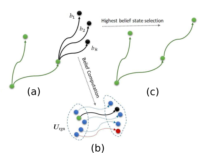
The proposed approach considers the above stated motion planning problem as an open-loop problem, i.e., it tries to develop a robust strategy that absorbs the potential deviations in the objects poses and in the results of the interactions occurring during the planning process. The work presents a physics-based motion planner with an underlying sampling-based kinodynamic planner that incorporates a robust tree growing strategy. This strategy works in two phases. The first one is a control sampling phase, once the state from which the tree will grow is selected, the algorithm applies randomly sampled controls called candidate controls for some randomly sampled time durations to generate valid motions called candidate motions (as depicted in Fig. 1-a). No uncertainty is considered in this phase. The second phase considers the uncertainty in the system, as stated in Sec. III-C, to compute the belief about the robustness and validity of the candidate motions. This is done for each candidate motion by considering the uncertainty and repeatedly applying the candidate control to obtain a set of associated motions, called particle motions (as shown in Fig. 1-b, where $\bm{U}_{\textrm{rgn}}$ represents the uncertainty in the object’s pose as introduced in Sec. IV-C2), and evaluating their validity. This belief is used to select the best candidate motion (Fig. 1-c), thus enhancing the tree exploration process. Additionally, a strategy to handle the uncertainty due to dynamic interaction is included in the approach.

IV-B Kinodynamic Motion Planning

Kinodynamic Motion Planning by Interior and Exterior Cell Exploration (KPIECE) [25, 10] is used to plan the trajectory. It is a sampling-based kinodynamic motion planner, particularly designed for systems with complex dynamics. A recent benchmarking study [26] concluded that KPIECE is a very good choice (to plan efficiently) for physics-based motion planing.

KPIECE grows a tree of motions. A motion is defined as $\nu=(\bm{x},\bm{u},d)$, where $\bm{x}$ is the start state of the motion, $\bm{u}$ is the control vector that is applied at state $\bm{x}$ for a time duration $d$. A key feature of KPIECE is how it estimates coverage during exploration. In order to estimate the coverage, the state space is projected into a low-dimensional space that is partitioned into cells. As a result of the projection, motions are classified into cells (each cell can contain several motions). These cells are divided into interior and exterior, depending on whether neighboring cells are occupied or not. The tree growing procedure is based on first selecting a cell, then selecting a motion of that cell and a state pertaining to it, from where the tree will grow. The cell selection process for the tree growth is based on a parameter called importance (cells with high importance are preferred for expansion), defined for a cell $z$ as:

$$\textrm{Imp($z$)}=\frac{\log(\mathcal{I})\cdot score}{C_{\textrm{cell}}\cdot(1+|Neigh(z)|)\cdot Cov(z)}\textrm{,}$$ (6)

where $\mathcal{I}$ represents the planning iteration when the cell was added to the grid, $C_{\textrm{cell}}$ represents the number of times it has been selected, $Cov(z)$ represents the number of states in the cell, $|Neigh(z)|$ is the number of instantiated neighboring cells, and $score$ represents the exploration progress, a value that is computed by evaluating the increase in the total coverage and the time spent to achieve this increment in coverage (when expanding from the cell). Once the cell is chosen, a motion from that cell is selected using a half normal distribution (over the indices of the motions, ordered starting with the newest). Finally, a state is randomly picked from the selected motion and a new motion is sampled from that selected state. The process continues until the tree of motions reaches the goal state.

The current proposal extends this algorithm with:

1. Strategies to handle the propagation of objects’ pose uncertainty into future states resulting from robot-object or object-object interactions (Sec. IV-C).

2. A motion sampling strategy that samples motions to expand the tree and computes the belief about the robustness of the sampled motions (Sec. IV-D).

3. A tree exploration strategy to modify the cell and motion selection process according to these beliefs (Sec. IV-E).

The algorithm, inspired by the original KPIECE algorithm, is presented in Algorithm 1. As input it takes the initial state of the world $\mathcal{W}_{init}$, the uncertainty in the initial pose of the objects $\bm{U}_{\textrm{init}}$, a goal region $\mathcal{Q}_{goal}$, a time threshold $T_{max}$, the number of candidate motions $k$ to use, the number of particle motions $n_{p}$ to evaluate the robustness, the displacement threshold $d$ for evaluating interactions, and the validity constraints $C$ that are to be used by the state validity checker. It starts with $\nu_{0}$, a motion of zero duration representing the initial state.

Lines 1 to 3, 12 and 14 are the default steps of KPIECE. The contribution of the current proposal is implemented in function UpdatePoseUncertainty (line-13) that updates the object pose uncertainty (Sec. IV-C2), in function MotionSampler (line-8) that samples $k$ motions and select the one that has highest belief (Sec. IV-D), and in functions SelectMotion (line-7) and UpdateCellImportance (line-15) that, respectively, select a motion from the selected cell to grow the tree and update the cell importance (Sec. IV-E).

inputs : Initial State $\mathcal{W}_{init}$, initial pose uncertainty $\bm{U}_{\textrm{init}}$, goal region $\mathcal{Q}_{goal}$, maximum time $T_{max}$, candidate motions $k$, particle motion $n_{p}$, displacement threshold $d$, validity constraints $C$

output : A sequence of motions that move the robot to the goal region

1 $\nu_{0}$ = $\mathcal{W}_{\textrm{init}}$

2 $G$.empty()

3 $G$.AddMotion($\nu_{0}$)

4 $\bm{U}_{\textrm{rgn}}=\bm{U}_{\textrm{init}}$

5 while $T_{max}$  do

6       cell = SelectCell($G$)

7       $\nu$= SelectMotion(cell)

8       $\nu_{new}$=MotionSampler($\nu,k,n_{p},d,C,\bm{U}_{\textrm{rgn}}$)

9       if $\nu_{new}\in Q_{goal}$ then

10             return path to $\nu_{0}$

11            

12      if $\nu_{new}!=$NULL then

13             $G$.AddMotion($\nu_{new}$)

14             $\bm{U}_{\textrm{rgn}}\leftarrow$UpdatePoseUncertainty($\bm{U}_{\textrm{rgn}}$)

15            

16      UpdateParameters()

17       UpdateCellImportance(cell)

return NULL

Algorithm 1 Probabilistic KPIECE

IV-C Handling Uncertainty Propagation

To handle uncertainty, the most robust motion should be chosen, i.e., those with higher chance to reach a valid state. For this purpose, the robustness of the candidate motions is evaluated by generating a set of particle motions. The belief of the candidate motions is computed as a function of the validity of the motion particles. This section explains how the particle motions are generated and used to update the uncertainty pose of the objects when interactions take place.

IV-C1 Particle Motion Generation

Particle motions are generated to evaluate a nominal candidate motion. Each particle motion is generated by sampling the initial state, the dynamic interaction parameters and the control to be applied: a) the initial state is sampled from the PDF function associated to the initial state of the nominal candidate motion (initially represented by Eq. (2)); b) the dynamic parameters are sampled using the PDF function described in Eq. (5); c) the control is determined by randomly adding noise to the nominal candidate control using Eq. (4). Then, a particle motion is obtained by applying the selected control to the chosen initial state and considering the sampled dynamic interaction parameters. Each particle motion will be evaluated using the state validity checker $\mathcal{F}$.

IV-C2 Updating Object Pose Uncertainty

Once interactions take place, the object pose uncertainty of the displaced objects is recomputed (objects may collide several times with the robot and/or with other objects). The poses of the objects as a result of interaction are highly variant depending on the contact regions and interaction force directions. Therefore, the resultant poses of the objects after applying several particle motions, can be modelled using the Gaussian Mixture Model (GMM), which is a convenient way to model the data that comes from different sources [27]:

$$\bm{U}_{\textrm{rgn}}=\sum_{j=1}^{n}\alpha_{j}\cdot\mathcal{N}(c_{j},m_{j})\;\textrm{with}\;\alpha_{j}\geq 0\;\textrm{,}\;\sum_{j=1}^{n}\alpha_{j}=1.$$ (7)

Eq. (7) is computed using Expectation-Maximization (EM) algorithm.

1 $\mathcal{M}\leftarrow$SampleCandidateMotions$(\nu,k)$

2 foreach $\nu_{i}\in\mathcal{M}$ do

3      $\mathcal{W}_{c}\leftarrow\textrm{{\sf\small Propagate}}^{c}$$(\nu_{i})$

4       if StateValidityChecker$(\mathcal{W}_{c},C)$ then

5             $\bm{v}_{\textrm{state}}=\bm{v}_{\textrm{int.}}=0$

6             for $j=1\;to\;n_{p}$ do

7                   $\rho\leftarrow$GetObjectPoses($\mathcal{W}_{c}$)

8                   SampleObjectPose($\rho,\bm{U}_{\textrm{rgn}}$)

9                   SampleDynamicParameters($\bm{U}_{\mathcal{D}}$)

10                   $\mathcal{W}_{p}\leftarrow\textrm{{\sf\small Propagate}}^{p}$($\nu_{i})$

11                   $valid_{S}\leftarrow$StateValidityChecker$(\mathcal{W}_{p},C)$

12                   $valid_{I}\leftarrow$InteractionEvaluator$(\mathcal{W}_{p},disp,d)$

13                   if $valid_{S}$ then

14                        $\bm{v}_{\textrm{state}}=\bm{v}_{\textrm{state}}+1$

15                  if $valid_{I}$ then

16                        $\bm{v}_{\textrm{int.}}=\bm{v}_{\textrm{int.}}+1$

17                  

18            $\bm{P}^{i}_{state}\leftarrow\bm{v}_{\textrm{state}}/n_{p}$

19             $\bm{P}^{i}_{int.}\leftarrow\bm{v}_{\textrm{int.}}/n_{p}$

20             $\bm{b}_{\nu_{i}}\leftarrow$ComputeBelief$(\bm{P}^{i}_{state},\bm{P}^{i}_{int.})$

21             AddMotionBelief$(\nu_{i},\bm{b}_{\nu_{i}})$

22             ExistValidMotion=$true$

23            

24      

25if ExistValidMotion then

26       if $\textrm{GenerateRandom(0,1)}>\textrm{bias}$ then

27             return $\bm{\nu}_{i}\leftarrow$SelectMotion(max($\bm{b}_{\bm{\nu}_{i}}$))

28      return $\bm{\nu}_{i}\leftarrow$SelectRandom($\mathcal{M}$)

return NULL

Algorithm 2 MotionSampler$(\nu,k,n_{p},d,C,\bm{U}_{\textrm{rgn}})$

IV-D Probabilistic Motion Sampler

The function MotionSampler (Line-8, Algorithm 1) is used to select a robust motion to expand the tree. It is a probabilistic motion sampler that samples $k$ candidates, computes the belief abut their validity, and returns the one that has the highest belief to be added to the tree data-structure. The process is summarized in Algorithm 2 and uses the following functions:

• SampleCandidateMotions: Samples a set $\mathcal{M}$ of $k$ candidate motions by first randomly choosing a single state from the input motion, and then by randomly sampling $k$ controls and durations.

• $\textrm{{\sf\small Propagate}}^{c}$: Uses Eq. (1) to compute the state resulting from applying motion $\nu_{i}$ (i.e., sampled control $\bm{u}$ at the selected state $\bm{x}$ for the time duration $d$).

• $\textrm{{\sf\small Propagate}}^{p}$: Uses Eq. (3) to compute the state resulting from applying motion $\nu_{i}$.

• StateValidityChecker: Evaluates the resultant state of the world, $\mathcal{W}_{c}$, using the state validity checker $\mathcal{F}$. If $\mathcal{W}_{c}$ satisfies all the validity constraints, $\mathcal{F}$ will return true, and false otherwise. The validity constraints are explained in Sec. III-B.

• GetObjectPoses: Retrieves the object poses from $\mathcal{W}_{c}$.

• SampleObjectPose: Samples the object poses using Eq.(2) or Eq.(7), depending on whether the object is still at its initial pose or has been moved due to interactions.

• SampleDynamicParameters: Samples the dynamic parameters using the probability distribution function described in Eq.(5).

• InteractionEvaluator: Returns true if $|disp|\leq d$ or false otherwise, where $disp$ is the displacement vector containing the displacement(s) covered by the object(s) in the result of interaction and $d$ a given threshold (experiments showed an increase in success rate if object pose uncertainty was reduced by avoiding very large displacements in highly cluttered scenes).

• ComputeBelief: Compute the belief of a motion as $b^{i}=\bm{\textrm{P}}^{i}_{state}\bm{\textrm{P}}^{i}_{int.}$.

• AddMotionBelief: Add the belief into the corresponding motion data structure in $\mathcal{M}$.

• SelectMotion: Selects the motion from $\mathcal{M}$ that has the highest belief, although with a given small probability, it is replaced by SelectRandom that selects a motion randomly regardless of its belief value.

IV-E Tree Exploration Strategy

The main parameters that control the tree exploration in KPIECE are the cell selection process and the motion selection from the selected cell. In order to enhance the exploration strategy to make the tree to grow through robust regions, our approach modifies these processes as follows.

• The definition of a motion is modified by incorporating the motion belief, i.e., $\bm{\nu}=(\mathcal{W},\bm{u},d,\bm{b}_{\nu})$, where $\mathcal{W}$ is the state of the world and $\bm{b}_{\nu}$ represents the belief about the robustness of $\nu$.

• A belief value is associated with the cells, according to the beliefs of the motions they contain. It is computed as the mean value of the beliefs of the motions normalized for all the cells, i.e.:

  $$\bm{b}_{cell}=\frac{\overline{\bm{b}}_{\nu}}{\sum_{\forall\textrm{cell}j}\overline{\bm{b}}_{\nu}^{j}}\;\;\;\textrm{with}\;\;\;\overline{\bm{b}}_{\nu}=\frac{1}{n}\sum_{\forall\nu_{i}\in\textrm{cell}}\bm{b}_{\nu_{i}}$$ (8)

• The Imp parameter is modified by integrating $\bm{b}_{\textrm{cell}}$ in order to favour those cells with higher belief (the strength of this bias being controlled by a heuristic parameter $f$, set equal to the number of cells):

  $$\textrm{Imp($z$)}=\frac{(1+f\bm{b}_{cell})\cdot\log{(\mathcal{I})}\cdot score}{C\cdot(1+|Neigh(z)|)\cdot Cov(z)}$$ (9)

Then, once a cell is chosen for the exploration, the motion from that cell is selected based on $\bm{b}_{\nu}$. If several motions have the same belief, a random motion will be selected from them. In order to explore the less certain regions, with a fixed small probability, the selection is done as in the standard KPIECE.

V Evaluation

The proposed approach described in the previous section results in a planner that enhances the power of KPIECE by considering uncertainty, object interactions and by favoring the tree exploration towards safer areas, allowing to plan motions in cluttered and uncertain environments. The main parameters of the algorithm are evaluated in this section, where comparisons with other approached are also done.

V-A Simulation Setup

The simulation setup is implemented in The Kautham Project [28], a C++ based open-source tool for motion planning. It provides the flexibility to plan under geometric, kinodynamic and physics-based constraints. It uses Open Motion Planning Library (OMPL) [29] as a core set of sampling-based planning algorithms. OMPL provides the integration with the Open Dynamic Engine that can be used as state propagator to handle the physics-based constraints. A variant of KPIECE has been implemented that includes all the extensions described above. All experiments were run on an Intel Core i7-4500U 1.80GHz CPU with 16 GB memory.

Figure 2: Sequence of the snapshots of the execution with: a) YuMi; b) Kuka-LWR. Videos: https://goo.gl/RzLVi1 and https://goo.gl/socxhb

Figure 3: Sequence of snapshots of the execution on the real YuMi robot. Video: https://goo.gl/bHspjZ

Figure 4: Histogram of average number of states and cells of 60 runs.

Figure 5: Graph of average planning time of 30 runs by varying the clutterness.

Figure 6: Graph of average planning success rate of 30 runs by varying the clutterness.

Figure 7: Graph of average planning time of 60 runs by varying the number of particle motions.

Figure 8: Graph of average planning success rate of 60 runs by varying the number of particle motions.

Figure 9: Histogram of average planning time of 60 runs by varying the cell size.

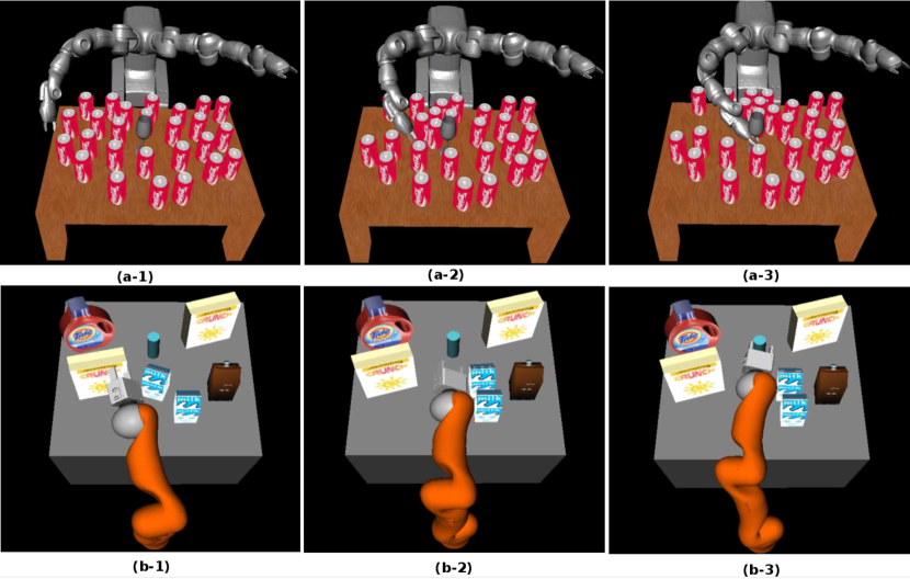
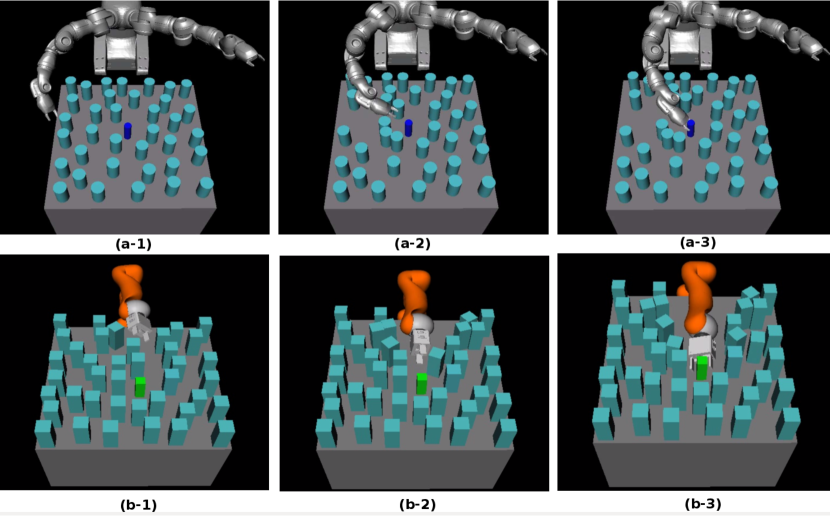
The proposed approach has been tested with two different robots: the 14 degree-of-freedoms (DOF) ABB YuMi and the 7 DOF KUKA-LWR, both of them with 2-finger grippers. The example scenarios are presented in Fig. 2. The scene shown in Fig 2-a consists of movable objects (red cans) and the target object (wine glass). The goal is to move the robot to a pre-grasp configuration to grasp the wine glass, by pushing away those cans obstructing the path. The scene depicted in Fig 2-b consists of movable objects of arbitrary shapes (boxes and bottle) and the target object (cyan cylinder). Moreover, the approach is also validated with the real YuMi robot, and a sequence of snapshots of the execution is depicted in Fig. 3.

V-B Benchmarking

The current approach is benchmarked against two approaches: 1) an ontological physics-based motion planner, introduced in [30], that enhances KPIECE for physics-based motion planning (it will be referred as o-KPIECE); 2) a task and motion planning approach for grasping in clutter proposed in [2, 3]. We run 30 simulation for each scenario.

V-B1 Algorithmic Parameter Evaluation

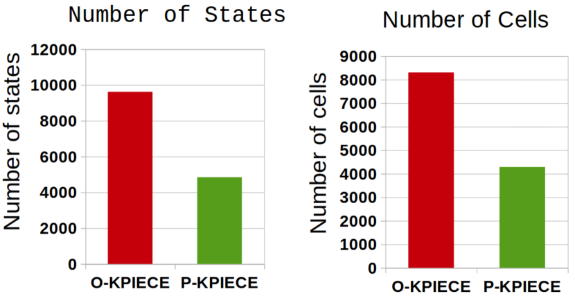
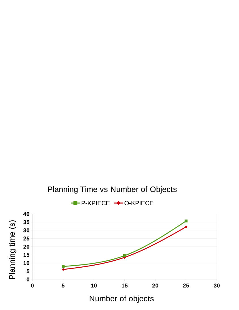
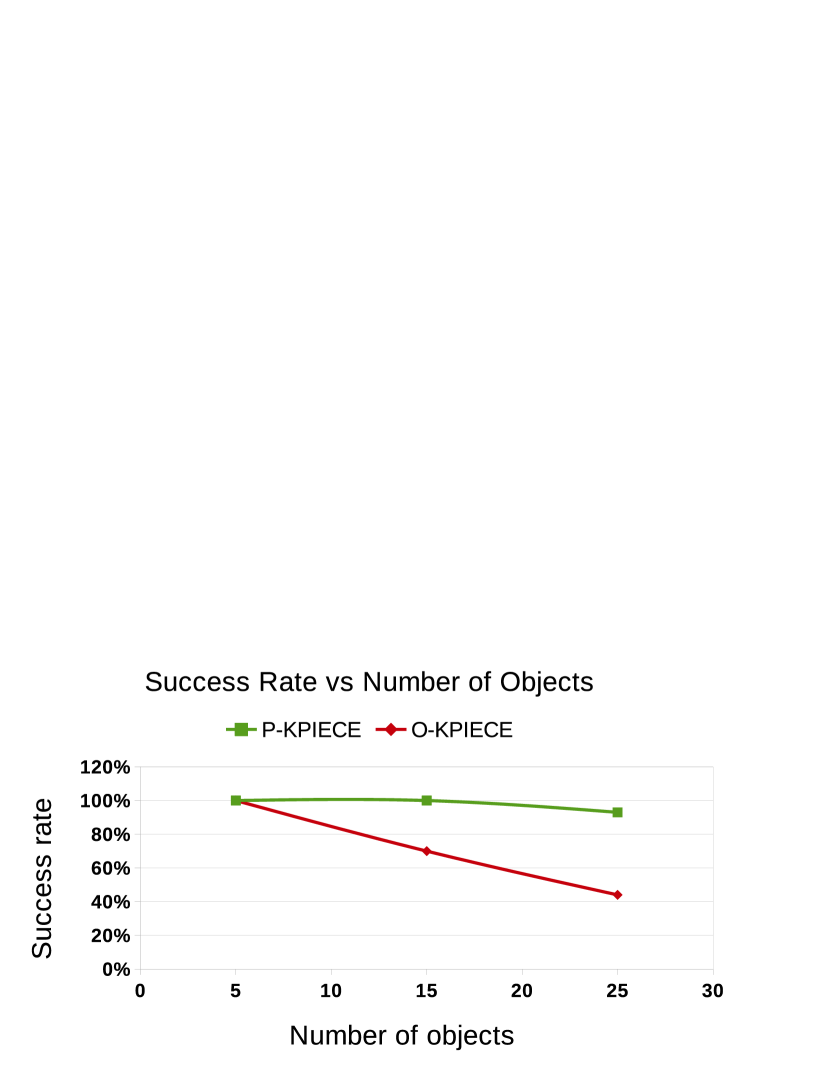
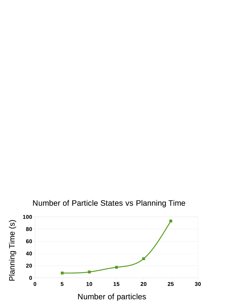
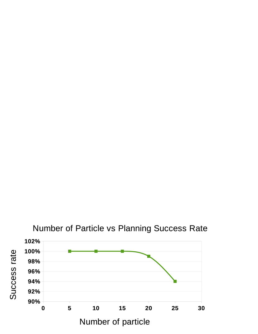
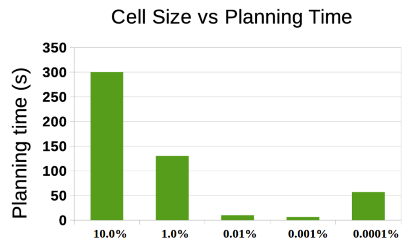
The current approach always generates more efficient solutions in terms of memory. Extensive tests showed that the number of generated states in p-KPIECE is always less than o-KPIECE. This implies that the number of generated cells is also less. Since the cell parameters are updated after each propagation step, p-KPIECE will update them faster, as compared to o-KPIECE. Fig. 9 shows the histograms of the average number of generated states and cells during planning, using o-KPIECE and p-KPIECE. The comparison between planning time of both planners using different levels of clutterness is shown in Fig. 9. Since p-KPIECE considers uncertainty, it performs an additional step that is robustness evaluation of each generated state, which makes it computationally expensive as compared to the o-KPIECE. As a result, for clutter scenes, the planning success rate of p-KPIECE is higher, as shown in Fig. 9. The robustness evaluation depends on the number of particle motions that are used to compute the belief, the larger the number of particle motions the more robust the plan. However, the computational time increases with the number of particle motions, shown in Fig. 9, and this may drop the planning success rate for not being able to find a solution on time, as shown in Fig. 9. Another parameter that may affect the planning process is the cell size used by KPIECE, that must be properly set. Big cell sizes do not ease the identification of the relevant regions of the workspace and fail to guide the tree growth, resulting in long unrealistic paths. On the other hand, smaller cell sizes better guide the search, thus enhancing the planning efficiency. Too small cell sizes, however, may increase the computational time required due to the huge number of cells generated. This effect on the planning time is depicted in Fig. 9, where cell size is represented as a percentage of the side length with respect to the side of the cube that models the workspace. In this work the state space is projected to the workspace, using the end-effector position.

V-B2 Comparison with Task Planning

The current proposal is also compared with the task and motion planning approaches (TMP) for grasping in the clutter without and with uncertainty  [3, 2], respectively. We have generated a qualitatively similar setup as that in those references, as shown in Fig. 10. Since the TMP approach presented in [2] does not consider uncertainty in the environment, in order to be fair with the comparison, we have assumed that the uncertainty in the environment is almost negligible, and then one particle motion is enough to evaluate the robustness, i.e., $k=1$. Whereas, to compare with [3], the value of $k$ is set to 15. The higher the value of $k$ the higher the confidence in the planner exploring safer regions, but the lower the computationally efficiency. The chosen value will depend on the problem; $k=15$ worked well in the example scenarios presented in this paper. Table I summarizes the results of the comparison. The data regarding the TMP approaches has been obtained from [2] and  [3], being generated with an Intel Core i7-4770K machine with 16 GB RAM (i.e., a faster processor than the one used in the current study). The task and motion planning approach requires explicit reasoning to perform each action, i.e. repeatedly selects an object to pick, computes the collision free trajectory to grasp it, finds and appropriate placement location and moves the object to that location. In contrast, the current proposal does not require explicit reasoning about the complex dynamic multi-body interactions for moving in the clutter. At each step, the objects must satisfy the global set of constraints, that are easy to evaluate. This process makes it easy to compute the robust plan efficiently, even in the presence of uncertainty.

Figure 10: Sequence of the snapshot of the executions with the YuMi and the Kuka-LWR, for the comparison with the task and motion planning approach. Videos: https://goo.gl/ZorqCF and https://goo.gl/F4fZVL

Obj.	Success rate %				Av. planning time (s)
	TP	TPU	pKP	pKPU	TP	TPU	pKP	pKPU
5	-	95	100	100	-	89	2.89	9.88
10	-	95	100	100	-	162	5.96	14.52
15	100	83	100	90	32	135	9.15	29.43
20	94	70	100	86	57	229	16.78	47.61
25	90	68	96	73	69	166	26.09	72.28
30	84	48	90	66	77	122	41.21	103.07
35	67	-	73	53	41	-	49.62	134.94
40	63	-	60	40	68	-	71.64	182.19

TABLE I: Comparison of p-KPIECE with task and motion planning approaches. Obj. represents the number of objects used, TP and TPU represent the approaches presented in [2] and [3], respectively. pKP and pKPU represent the p-KPIECE with and without uncertainty, respectively.

V-C Qualitative Analysis

The quality of the solution path computed by p-KPIECE is improved as compared to the o-KPIECE. Since o-KPIECE does not evaluate the post-effect of dynamic interactions and the results of object-object interactions, that leads to the unreasonable results. For cluttered scenes, in most of the cases, it displaces the target object or drops the objects from the table surface, whereas p-KPIECE carefully evaluates the post-effect of dynamic interactions, interaction velocity and displacement covered by the object in the result of interactions, greatly increasing the planning success rate. Moreover, the incorporation of robustness evaluation phase results in the more stable and robust motion plans, i.e. the integration of the results of robustness evaluation within the planning data structure allows the search to be guided towards the regions that are safer, thus increasing the success in the final execution of the planned paths.

The solution computed by p-KPIECE is also qualitatively different from the TMP solution. The TMP solution is generated by integrating several move, pick and place actions. Each motion planning query is set to move the robot to a particular place (for picking or placing an object); these local queries do not consider the final goal. In contrast, p-KPIECE computes the solution in a more natural way, it launches a single query and moves away the objects obstructing the path.

Currently, no smoothing operation over the trajectory is applied, although it can easily be added by using deterministic control sampling strategies or by applying post processing over the computed path as presented in [14].

VI CONCLUSIONS

This study proposes a randomized physics-based motion planner for planning the grasping motions in cluttered and unstructured environments. The developed framework takes into account the uncertainty in the objects’ pose and in the contact dynamics. The KPIECE planner is enhanced by: a) introducing a motion sampler, for the extension of the tree, that samples motions and evaluates the belief about their robustness in the presence of uncertainty; b) biasing the tree exploration strategy based on the computed beliefs. The proposed planner enables single actions to move multiple objects, thereby avoiding the combinatorial explosion in the task planning part of TMP. The work is validated in simulation and in real environment against other approaches, such as ontological physic-based motion planner and task and motion planning approach. The results show significant advantages in terms of planning time, success rate and the quality of the computed solution path.

References

- [1] N. T. Dantam, Z. K. Kingston, S. Chaudhuri, and L. E. Kavraki, “Incremental task and motion planning: A constraint-based approach,” in Robotics: Science and Systems, 2016, pp. 1–6.
- [2] S. Srivastava, E. Fang, L. Riano, R. Chitnis, S. Russell, and P. Abbeel, “Combined task and motion planning through an extensible planner-independent interface layer,” in IEEE International Conference on Robotics and Automation, 2014, pp. 639–646.
- [3] D. Hadfield-Menell, E. Groshev, R. Chitnis, and P. Abbeel, “Modular task and motion planning in belief space,” in IEEE/RSJ International Conference on Intelligent Robots and Systems, 2015, pp. 4991–4998.
- [4] M. Stilman and J. J. Kuffner, “Navigation among movable obstacles: Real-time reasoning in complex environments,” International Journal of Humanoid Robotics, vol. 2, no. 04, pp. 479–503, 2005.
- [5] M. Stilman, J.-U. Schamburek, J. Kuffner, and T. Asfour, “Manipulation planning among movable obstacles,” in IEEE International Conference on Robotics and Automation, 2007, pp. 3327–3332.
- [6] M. Dogar and S. Srinivasa, “Push-grasping with dexterous hands: Mechanics and a method,” in IEEE/RSJ International Conference on Intelligent Robots and Systems, 2010.
- [7] D. Mehmet and S. Siddhartha, “A framework for push-grasping in clutter,” Robotics: Science and systems VII, vol. 1, 2011.
- [8] M. Dogar, K. Hsiao, M. Ciocarlie, and S. Srinivasa, “Physics-based grasp planning through clutter,” in Robotics: Science and Systems, 2012.
- [9] M. Laskey, J. Lee, C. Chuck, D. Gealy, W. Hsieh, F. T. Pokorny, A. D. Dragan, and K. Goldberg, “Robot grasping in clutter: Using a hierarchy of supervisors for learning from demonstrations,” in IEEE International Conference on Automation Science and Engineering, Aug 2016, pp. 827–834.
- [10] I. Sucan and L. E. Kavraki, “A sampling-based tree planner for systems with complex dynamics,” IEEE Transactions on Robotics, vol. 28, no. 1, pp. 116–131, 2012.
- [11] Á. Sánchez-Miralles and M. Á. Sanz-Bobi, “Global path planning in gaussian probabilistic maps,” Journal of Intelligent and Robotic Systems, vol. 40, pp. 89–102, 2004.
- [12] A. Bry and N. Roy, “Rapidly-exploring random belief trees for motion planning under uncertainty,” in IEEE International Conference on Robotics and Automation, 2011, pp. 723–730.
- [13] S. M. LaValle and J. J. Kuffner, “Randomized kinodynamic planning,” The International Journal of Robotics Research, vol. 20, no. 5, pp. 378–400, 2001.
- [14] J. Van Den Berg, P. Abbeel, and K. Goldberg, “LQG-MP: Optimized path planning for robots with motion uncertainty and imperfect state information,” The International Journal of Robotics Research, vol. 30, pp. 895–913, 2011.
- [15] R. Alterovitz, T. Siméon, and K. Y. Goldberg, “The stochastic motion roadmap: A sampling framework for planning with markov motion uncertainty,” in Robotics: Science and systems, 2007, pp. 233–241.
- [16] N. A. Melchior and R. Simmons, “Particle RRT for path planning with uncertainty,” in IEEE International Conference on Robotics and Automation, 2007, pp. 1617–1624.
- [17] A. M. Johnson, J. King, and S. Srinivasa, “Convergent planning,” IEEE Robotics and Automation Letters, vol. 1, no. 2, pp. 1044–1051, July 2016.
- [18] J. E. King, V. Ranganeni, and S. S. Srinivasa, “Unobservable monte carlo planning for nonprehensile rearrangement tasks,” in IEEE International Conference on Robotics and Automation, May 2017, pp. 4681–4688.
- [19] Muhayyuddin, A. Akbari, and J. Rosell, “-PMP: Enhancing physics-based motion planners with knowledge-based reasoning,” Journal of Intelligent & Robotic Systems, Sep 2017. [Online]. Available: https://doi.org/10.1007/s10846-017-0698-z
- [20] J. A. Haustein, J. King, S. S. Srinivasa, and T. Asfour, “Kinodynamic randomized rearrangement planning via dynamic transitions between statically stable states,” in IEEE International Conference on Robotics and Automation, 2015, pp. 3075–3082.
- [21] J. E. King, M. Cognetti, and S. S. Srinivasa, “Rearrangement planning using object-centric and robot-centric action spaces,” in IEEE International Conference on Robotics and Automation, May 2016, pp. 3940–3947.
- [22] A. Cosgun, T. Hermans, V. Emeli, and M. Stilman, “Push planning for object placement on cluttered table surfaces,” in IEEE/RSJ International Conference on Intelligent Robots and Systems, Sept 2011, pp. 4627–4632.
- [23] M. Gupta, J. Müller, and G. S. Sukhatme, “Using manipulation primitives for object sorting in cluttered environments,” IEEE Transactions on Automation Science and Engineering, vol. 12, no. 2, pp. 608–614, April 2015.
- [24] J. Mahler and K. Goldberg, “Learning deep policies for robot bin picking by simulating robust grasping sequences,” in 1st Conference on Robot Learning, 2017.
- [25] I. A. Şucan and L. E. Kavraki, “Kinodynamic motion planning by interior-exterior cell exploration,” in Algorithmic Foundation of Robotics VIII. Springer, 2009, pp. 449–464.
- [26] M. Gillani, A. Akbari, and J. Rosell, “Physics-based motion planning: Evaluation criteria and benchmarking,” in Robot 2015: Second Iberian Robotics Conference. Springer, 2016, pp. 43–55.
- [27] P. Pfaff, C. Plagemann, and W. Burgard, “Gaussian mixture models for probabilistic localization,” in IEEE International Conference on Robotics and Automation, May 2008, pp. 467–472.
- [28] J. Rosell, A. Pérez, A. Aliakbar, Muhayyuddin, L. Palomo, and N. García, “The kautham project: A teaching and research tool for robot motion planning,” in IEEE International Conference on Emerging Technologies and Factory Automation, 2014.
- [29] I. A. Şucan, M. Moll, and L. E. Kavraki, “The Open Motion Planning Library,” IEEE Robotics & Automation Magazine, vol. 19, no. 4, pp. 72–82, December 2012.
- [30] Muhayyuddin, A. Akbari, and J. Rosell, “Ontological physics-based motion planning for manipulation,” in IEEE International Conference on Emerging Technologies Factory Automation, 2015, pp. 1–7.