Review of recent developments in the random–field Ising model

Abstract

A lot of progress has been made recently in our understanding of the random–field Ising model thanks to large–scale numerical simulations. In particular, it has been shown that, contrary to previous statements: the critical exponents for different probability distributions of the random fields and for diluted antiferromagnets in a field are the same. Therefore, critical universality, which is a perturbative renormalization–group prediction, holds beyond the validity regime of perturbation theory. Most notably, dimensional reduction is restored at five dimensions, i.e., the exponents of the random–field Ising model at five dimensions and those of the pure Ising ferromagnet at three dimensions are the same.

I Introduction

The random–field Ising model (RFIM) is the simplest disordered system. Its Hamiltonian is

$$\mathcal{H}=-J\sum_{\langle xy\rangle}\sigma_{x}\sigma_{y}-\sum_{x}h_{x}\sigma_{x},$$ (1)

where $\sigma_{x}=\pm 1$ on a hypercubic lattice in $D$ dimensions with nearest–neighbor ferromagnetic interactions. The $h_{x}$ are independent random magnetic fields obeying different probability distributions. The RFIM has a long history. Let us remind some of the most important results.

The perturbative renormalization group (PRG) can be carried out to all orders of perturbation theory (in fact this is the only known case where PRG can be carried to all orders). It predicts dimensional reduction and supersymmetry Aharony ; Y ; PS1 . This means that the critical exponents of the RFIM in $d$ dimensions are the same as the exponents of the pure Ising model in $d-2$ dimensions. It has been proven that dimensional reduction is not true in three dimensions BK .

There are some other open questions we would like to address in this paper. What about other predictions of PRG? Are some predictions still true? What about higher dimensions? Why PRG breaks down at three dimensions? There have been recently very large–scale simulations which clarify these questions. The main conclusions are: contrary to previous statements universality is true in three, four, and five dimensions. Diluted antiferromagnets in a field are in the same universality class with the RFIM. PRG breaking is a low–dimensional phenomenon. PRG and dimensional reduction are restored at five dimensions. There is a maximum violation of self–averaging in the distribution of low lying excited states near the critical point.

II Universality

The explanation of critical universality is a major success of the renormalization group. In the case of the RFIM, PRG predicts that different random–field Ising models, where the random fields are drawn from different probability distributions, belong to the same universality classes. Also, more surprisingly, diluted antiferromagnets in a field are predicted to belong to the same universality class. These two predictions have been recently shown numerically to be true in three, four, and five dimensions FMMa ; FMMb ; PiS ; FMMPSa ; FMMPSa2 ; FMMPSb , despite the failure of PRG. Previous numerical simulations are incompatible with these predictions for universality.

Because of these older simulations, the prevailing view was that universality is not valid for the RFIM because of the failure of PRG. This view has changed thanks to recent simulations by Fytas and Martín-Mayor FMMa ; FMMb . They considered double Gaussian (considering also the bimodal and Gaussian limits) and Poissonian random–field distributions in three dimensions. They found the same exponents for all distributions of the random fields.

What explains the disagreement with previous work? Subdominant corrections to scaling. For finite sizes there is no simple power–law behavior near the critical point. There are subdominant corrections to single power–law behavior. Large lattice sizes and high–precision data are needed in order to measure the subdominant corrections to scaling. Fytas and Martín-Mayor simulated systems with linear sizes up to $L=196$ and $10^{7}$ samples per size. Furthermore you need the appropriate theoretical framework in order to analyze these corrections.

In field theory, subdominant corrections are controlled by the Callan–Symanzik $\beta(g)$ function. $\omega=\left.\frac{\mathrm{d}\beta}{\mathrm{d}g}\right|_{g=g^{\ast}}$ is a universal exponent and controls the leading corrections to scaling. The same exponent, $\omega$, controls corrections to scaling for all observables. When you have good enough data allowing you to compute those non–leading corrections, you find that all considered probability distributions of the random fields have the same exponents, thus confirming universality.

Subsequently Picco and Sourlas PiS , using the same methods, have shown that the three-dimensional diluted antiferromagnets in a field belong to the same universality class with the RFIM, contrary to previous assertions. Fytas et al., computed critical exponents at four and five dimensions for both the Gaussian and Poissonian distributions. Exponents are the same for both distributions and universality is valid also at four and five dimensions, see Refs. FMMPSa ; FMMPSa2 ; FMMPSb . Universality is of course not only valid in PRG but is a general property of the renormalization group, but it is in general very hard to show that two different physical systems belong to the same universality class except by using the PRG. This is particularly the case of the RFIM.

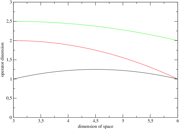
Figure 1: (color online) Pictorial representation of the non–crossing mechanism that protects universality (see relevant discussion in the main text). The figure, which has an illustrative purpose only, depicts the operator dimension of three generic operators as a function of the dimension of space.

Why critical universality, as established by the PRG is valid in three dimensions while PRG is broken? In PRG, universality is established using Wilson’s operator product expansion and the $\epsilon$ expansion, i.e. close to the upper critical dimension, $D_{\rm u}=6$ in the case of the RFIM. One classifies the operators into relevant, marginal, or irrelevant according to their scaling dimensions. The scaling dimensions of the operators $D_{O}$ are functions of the dimension of space $d$. The $D_{O}(d)$’s change when the dimension of space is changed. A necessary and sufficient condition for non changing universality classes as the dimension of space $d$ varies is for the scaling dimensions $D_{O}(d)$ of the leading operators not to cross when the dimension of space is lowered from $d=D_{\rm u}$ down to $d=3$ as this is illustrated in Fig. 1.

If this is the case, the classification of operators into relevant, marginal, and irrelevant remains unchanged when the dimension of space is lowered.

The $\epsilon$ expansion computes the dimension of the operators and their derivatives with respect to $d$ at $d=D_{\rm u}$. Why the classification is it still valid for $\epsilon=3$ when PRG is broken? In fact we do not know of any case of the classification into universality classes using the $\epsilon$ expansion not been valid at lower dimensions. Why is this so?

The reason for the scaling dimensions of operators not to cross when the dimension of space decreases is probably the following Sourlas . Scaling dimensions of operators are eigenvalues of the scaling transformations, i.e. of the group of dilatations of space. It is well known from the early days of quantum mechanics that in the generic case the eigenvalues of operators, that is the eigenvalues of the matrices in their matrix representation, do not cross if one changes a single parameter LL . This phenomenon is called repulsion of eigenvalues. If universality is valid around $d=6$ dimensions there is big chance to be valid at $d=3$ dimensions because of eigenvalue repulsion. Validity of universality at three dimensions does not depend on the validity of PRG at this dimension. The previous argument can be inverted. If it is found by other means, like experiments or numerical simulations, that universality classes in three dimensions coincide with those established by the $\epsilon$ expansion, it means that PRG is valid near the upper critical dimension $D_{\rm u}$, i.e. the epsilon expansion is valid.

III Discussion on the dimensional reduction restoration

Recent numerical simulations computed the critical exponents for the Gaussian and Poissonian probability distributions of the random fields at four FMMPSa ; FMMPSa2 and five dimensions FMMPSb . It was found that PRG and dimensional reduction is violated at four dimensions. On the contrary our simulations are compatible with the validity of PRG and dimensional reduction in five dimensions. In five dimensions we simulated Gaussian and Poissonian random fields, for linear sizes $4\leq L\leq 28$ and $10^{7}$ samples per size. Numerical results for our estimates of critical exponents as a function of the space dimensionality are summarized in Fig. 2. In the main panel we show the cases for $\nu$, $\overline{\eta}$, and the violation of hyperscaling exponent $\theta=2-\overline{\eta}+\eta$ FMMPSa2 . In the corresponding inset we present the anomalous dimension $\eta$ on its own for clarity reasons.

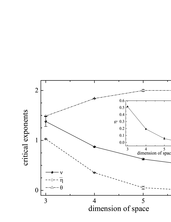
Figure 2: Numerical estimates of critical exponents as a function of the dimension of space for the $3d$ FMMa , $4d$ FMMPSa ; FMMPSa2 , and $5d$ RFIM FMMPSb . The data points corresponding to $d=6$ are the mean–field exponents.

The most compelling evidence comes from fitting the data assuming dimensional reduction, i.e. assuming that the critical exponents of the RFIM in five dimensions are equal to those of the pure Ising model in three dimensions, which are known very precisely. As all the exponents are assumed to be known there are very few parameters to fit. The quality of the fit, $\chi^{2}$ per degree of freedom, is excellent: $3.43/7$ for $\nu$, $13.37/11$ for $\eta$, and $4.15/7$ for the difference $2\eta-\overline{\eta}$. We conclude that PRG and dimensional reduction are restored at five dimensions and that the breaking of PRG is a low–dimensional phenomenon. Tarjus et al. Tar1 ; Tar2 ; Tar3 using functional renormalization group, also argue that dimensional reduction is restored for dimensions larger than $5.1$.

Why PRG is valid at higher dimensions? What is the reason of PRG failure at low dimensions? As PRG is valid at all orders of perturbation theory, the reason of its breaking must be non perturbative. Parisi and Sourlas PS0 proposed that the reason is the formation of bound states, which is a non perturbative phenomenon. The mass of the bound state provides a new length scale which is not taken into account in the traditional PRG analysis.

The argument for the formation of bound states is the following: first Kardar et al. K1 ; K2 observed that interactions among replicas are attractive – this is not the case for branched polymers and dimensional reduction holds in that case. For the random interface problem they computed the spectrum of the effective Hamiltonian with Bethe ansatz and found the lowest states to be bound states. Then Brézin and De Dominicis BDD1 ; BDD2 wrote the Bethe–Salpeter equation for $\langle s^{\alpha}s^{\beta}(0)s^{\alpha}s^{\beta}(x)\rangle$ in the RFIM, where $\alpha$ and $\beta$ are two different replica indices and they found an instability in the Bethe–Salpeter kernel for $d<6$ most probably implying the existence of bound states. As remarked by Parisi Pa83 ,

$$\langle s^{\alpha}(0)s^{\alpha}(x)\rangle=\overline{\langle\sigma(0)\sigma(x)\rangle},$$ (2)

where $\overline{\langle\sigma(0)\sigma(x)\rangle}$ is the average over samples of $\langle\sigma(0)\sigma(x)\rangle$, and

$$\langle s^{\alpha}s^{\beta}(0)s^{\alpha}s^{\beta}(x)\rangle=\overline{(\langle\sigma(0)\sigma(x)\rangle)^{2}},$$ (3)

where the replica indices $\alpha\neq\beta$.

Figure 3: (Color online) Illustration of the probability distribution $P(dm,dj,\delta h,L)$ for $dj=0$. Left panel: $L=60$ and two values of $\delta h$. Right panel: $L=60$, $L=120$ and $\delta h=0.45L^{-\gamma/\nu}$.

Parisi and Sourlas PS0 found that for large $x$ in three dimensions

$$\overline{\langle\sigma(0)\sigma(x)\rangle}\sim\exp{(-mx)}$$ (4)

and

$$\overline{(\langle\sigma(0)\sigma(x)\rangle)^{2}}\sim\exp{(-mx)}$$ (5)

with the same $m$! $m$ is the mass of the intermediate state with the lowest mass. This means that there exists a state in replica field theory that couples to both the $s^{\alpha}(x)$ and $s^{\alpha}s^{\beta}(x)$ operators. Not such state exists in perturbation theory. They concluded to the existence of a new state, not present in perturbation theory, which couples to both $s^{\alpha}(x)$ and $s^{\alpha}s^{\beta}(x)$. This must be a bound state, in agreement with Brézin and De Dominicis. They also pointed out that the space dimension plays a crucial role in the formation of bound states. In the formation of bound states there is a competition between the attractive forces and the size of the available phase space. The size of phase space increases with the dimension of space making the formation of bound states more difficult in higher dimensions. We expect that for high enough dimensions bound states will no longer exist, and PRG predictions should hold. This argument does not predict at which dimension PRG is restored.

Another remarkable fact is the maximum violation of self–averaging in the sample to sample fluctuations, as explained below. In order to compute the magnetic susceptibility, one can add a small translation invariant magnetic field $\delta h$. For each sample compute $m_{0}$, the ground–state magnetization at $J=J_{\rm c}+dj$, where $J_{\rm c}$ denotes the critical point, add $\delta h$ and find the new ground–state magnetization $m^{\prime}$. The resulting change of the ground–state magnetization due to $\delta h$ is $dm=m_{0}-m^{\prime}$.

Figure 4: (Color online) Illustration of the probability distribution $P(dm,dj,\delta h,L)$ for $dj=0.3L^{-1/\nu}$, $\delta h=2.2L^{-\gamma/\nu}$ (left panel) and $dj=0.6L^{-1/\nu}$, $\delta h=1.1L^{-\gamma/\nu}$ (right panel).

Consider the probability distribution $P(dm,dj,\delta h,L)$ of $dm$ over the random–field samples, see Fig. 3. The left panel of the figure shows $P(dm,dj,\delta h,L)$ of $dm$ for $dj=0$, i.e. at $J=J_{\rm c}$, for $L=60$ and two values of $\delta h$. We see it is a bimodal probability distribution. Increasing $\delta h$ only modifies the size of the two peaks. Note the bound $0\leq dm\leq 2$, implying that our bimodal distribution, with one of the peaks at $dm\sim 2$, is a maximum violation of self–averaging. The right panel of Fig. 3 illustrates $P(dm,dj,\delta h,L)$ of $dm$ for $dj=0$, i.e. at $J=J_{\rm c}$ for $L=60$ and $L=120$ and $\delta h=0.45L^{-\gamma/\nu}$. $\gamma$ is the critical exponent of the magnetic susceptibility. Clearly, $P(dm,dj,\delta h,L)$ obeys finite–size scaling.

The next two panels in Fig. 4 present $P(dm,dj,\delta h,L)$ for $dj=0.3L^{-1/\nu}$ and $\delta h=2.2L^{-\gamma/\nu}$, and $dj=0.6L^{-1/\nu}$ and $\delta h=1.1L^{-\gamma/\nu}$, respectively. Results for three different system sizes are shown, namely for $L=30$, $60$, and $L=90$.

We observe again strong violations of self–averaging, obeying finite–size scaling. They are not finite volume artifacts. We have no theoretical explanation of these maximal violations of self–averaging.

The reader might be puzzled by our findings of a bimodal distribution of $dm$ and at the same time the finite–size scaling relation $\frac{\mathrm{d}m}{\delta h}\sim L^{\gamma/\nu}$. This is possible, as it is illustrated by the toy model of the following bimodal probability distribution

$$p_{\rm toy}(dm,\delta h,L)=p_{0}\delta(dm)+p_{1}\delta(dm-c)\,;\quad\ p_{1}\sim\delta hL^{\gamma/\nu}\,;\quad\ p_{0}+p_{1}=1,$$ (6)

where $c$ is a constant and $\delta h$ is small. In this model $\langle(dm)^{k}\rangle\sim\delta hc^{k}L^{\gamma/\nu}$.

IV Conclusions

In summary, numerical simulations have provided a significant step forward in our understanding of the RFIM. The combination of an appropriate fluctuation–dissipation formalism with modern finite-size analysis FMMa ; FMMb has provided strong evidence for universality at space dimensions $d=3$ FMMa ; FMMb ; PiS , $d=4$ FMMPSa ; FMMPSa2 , and $d=5$ FMMPSb . The evidence for violations of basic predictions of the PRG, such as dimensional reduction, is crystal clear at $d=3$ and $d=4$. On the other hand, our rather accurate results at $d=5$ are compatible with dimensional reduction. Although universality is a prediction of the PRG, it is obvious that universality is valid outside of the perturbative regime. An argument based on eigenvalue-repulsion has been proposed to explain why universality is robust against non–perturbative effects Sourlas .

Nevertheless many open questions remain. Our results are based on numerical simulations with their inherent error bars. Even when error bars are very small they do not replace a mathematical proof. In particular we cannot exclude the possibility that PRG is broken for any $d<D_{\rm u}=6$ (a non–analytic dependence in $d-D_{\rm u}$, such as $\exp{[1/(d-D_{\rm u})]}$, cannot be excluded). It could also in theory be possible that such exponentially small contributions violate universality.

If bound states are responsible for the breaking of the PRG, one should introduce the fields representing these bound states and write the effective Hamiltonian in terms of these fields. We do not know what these fields are. This effective Hamiltonian can be very different than the original one. The relation between the fields of this Hamiltonian and the original ones can be very complicated. A well known example in this context is the sine–Gordon model where the effective field theory is the massive Thirring model mandelstam ; coleman ; mandelstam2 . The fermions of the massive Thirring model are exponential functions of the bosons of the sine–Gordon model.

- (1) A. Aharony, Y. Imry, and S.-K. Ma, Phys. Rev. Lett. 37, 1364 (1976).
- (2) A.P. Young, J. Phys. A: Math. Gen. 10, L257 (1977).
- (3) G. Parisi and N. Sourlas, Phys. Rev. Lett.43, 744 (1979).
- (4) J. Bricmont and A. Kupiainen, Phys. Rev. Lett. 59, 1829 (1987).
- (5) N.G. Fytas and V. Martín-Mayor, Phys. Rev. Lett. 110, 227201 (2013).
- (6) N.G. Fytas and V. Martín-Mayor, Phys. Rev. E 93, 063308 (2016).
- (7) M. Picco and N. Sourlas, Europhys. Lett. 109, 37001 (2015).
- (8) N.G. Fytas, V. Martín-Mayor, M. Picco, and N. Sourlas, Phys. Rev. Lett. 116, 227201 (2016).
- (9) N.G. Fytas, V. Martín-Mayor, M. Picco, and N. Sourlas, J. Stat. Mech. (2017) 033302.
- (10) N.G. Fytas, V. Martín-Mayor, M. Picco, and N. Sourlas, Phys. Rev. E 95, 042117 (2017).
- (11) N. Sourlas, arXiv:1706.07176 (2017).
- (12) see for instance: L.D. Landau and E.M. Lifshitz, Quantum Mechanics (Pergamon Press, 1965).
- (13) M. Tissier and G. Tarjus, Phys. Rev. Lett. 107, 041601 (2011).
- (14) M. Tissier and G. Tarjus, Phys. Rev. B 85, 104203 (2012).
- (15) G. Tarjus, I. Balog, and M. Tissier, Europhys. Lett. 103, 61001 (2013).
- (16) G. Parisi and N. Sourlas, Phys. Rev. Lett. 89, 257204 (2002).
- (17) M. Kardar, Nucl. Phys. B 290, 582 (1987).
- (18) E. Medina, M. Kardar, M. Shapir, and X.R. Wang, Phys. Rev. Lett. 62, 941 (1989).
- (19) E. Brézin and C. De Dominicis, Europhys. Lett. 44, 13 (1998).
- (20) E. Brézin and C. De Dominicis, Eur. Phys. J. B 19, 467 (2001).
- (21) G. Parisi, Phys. Rev. Lett. 50, 1946 (1983).
- (22) S. Mandelstam, Phys. Rev. D 11, 3026 (1975).
- (23) S. Coleman, Classical lumps and their quantum descendants, in: Aspects of Symmetry: Selected Erice Lectures, pp. 185-264 (Cambridge University Press, 1985).
- (24) S. Mandelstam, Phys. Rep. 23, 307 (1976).