An Analytic and Numerical Analysis of Weighted Singular Cauchy Integrals with Exponential Weights on $\mathbb{R}$

Abstract.

This paper concerns an analytic and numerical analysis of a class of weighted singular Cauchy integrals with exponential weights $w:=\exp(-Q)$ with finite moments and with smooth external fields $Q:\mathbb{R}\to[0,\infty)$, with varying smooth convex rate of increase for large argument. Our analysis relies in part on weighted polynomial interpolation at the zeros of orthonormal polynomials with respect to $w^{2}$. We also study bounds for the first derivatives of a class of functions of the second kind for $w^{2}$.

Keywords: Cauchy principal value integral; Exponential weight; Erdős weight, Freud weight, Numerical approximation, Orthogonal polynomial, Quadrature, Singular integral, Weighted approximation.

1. Introduction

Let $Q:\mathbb{R}\to[0,\infty)$ belong to a class of continuously differentiable functions with varying smooth convex rate of increase for large argument. For a class of exponential weight functions $w:=\exp(-Q)$ with finite moments, we investigate the weighted Cauchy principal value integral

$$H_{w^{2}}[f;x]:=-\!\!\!\!\!\!\!\!\;\int_{\mathbb{R}}w^{2}(t)\frac{f(t)}{t-x}dt=\!\lim_{\varepsilon\to 0+}\!\left(\int_{-\infty}^{x-\varepsilon}\!w^{2}(t)\frac{f(t)}{t-x}dt+\!\int_{x+\varepsilon}^{\infty}\!w^{2}(t)\frac{f(t)}{t-x}dt\right)$$

with respect to its analytical properties, and we develop and analyze numerical methods for the approximate calculation of such integrals.

Here, we work on the real line, i.e. $x\in\mathbb{R}$ is arbitrary but fixed and $f:\mathbb{R}\to\mathbb{R}$ belongs to a class of functions for which in particular, $H_{w^{2}}[f;x]$ is finite. When we say $w$ has finite moments, we mean that $\int_{\mathbb{R}}x^{n}w^{2}(x)<\infty$, ($n=0,1,2,...$). Notice that the numerator in the integrand of the operator $H_{w^{2}}[f,x]$ is $fw^{2}$.

One reason for our investigation is due to the fact that integral equations with weighted Cauchy principal value integral kernels have shown to be an important tool for the modelling of many physical situations. See for example [4, 6, 7, 8, 9, 15, 16, 18, 25] and the references cited therein. In the case of ordinary integrals (without strong singularities) on unbounded intervals, various interesting results can be found for example in [23, 28].

In a series of papers, [6, 7, 8, 9], the authors studied this problem and some of its applications for a class of weights $w:=\exp(-Q)$ with finite moments and with even external fields $Q:\mathbb{R}\to[0,\infty)$ belonging to a class of continuously differentiable functions with smooth polynomial rate of increase for large argument. An example of such an external field $Q$ studied is $|x|^{\alpha}$ where $\alpha>1$.

In this paper, we extend the results of [6] to a class of exponential weight functions $w=\exp(-Q)$ with finite moments and with external fields $Q:\mathbb{R}\to[0,\infty)$ continuously differentiable with certain convex increase for large argument. In particular, this class of external fields $Q$ studied need not be even (a considerably weaker condition on $Q$) and may allow for considerable varying convex rates of increase for large argument for example smooth polynomial increase and also faster than smooth polynomial increase. Typical examples [19, 22] of admissible external fields $Q$ would be with some $\beta\geq\alpha>1$ and $\ell,k\geq 0$,

$$Q_{1,\alpha,\beta}(x):=\begin{cases}x^{\alpha},&x\in[0,\infty)\\ |x|^{\beta},&x\in(-\infty,0)\end{cases}$$

or

$$Q_{2,\alpha,\beta,\ell,k}(x):=\begin{cases}\exp_{l}(x^{\alpha})-\exp_{l}(0),&x\in[0,\infty)\\ \exp_{k}(|x|^{\beta})-\exp_{k}(0),&x\in(-\infty,0)\end{cases}$$

Here, for $x\in\mathbb{R}$, $\exp_{0}(x):=x$ and for $j\geq 1$, $\exp_{j}(x):=\exp(\exp(\exp...\exp(x)))$, $j$ times is the $j$th iterated exponential. In particular, $\exp_{j}(x)=\exp(\exp_{j-1}(x))$.

1.1. A note on notation and constants

Throughout, $|.|$ is the Euclidean metric on $\mathbb{R}$. $\mathcal{P}_{n}$ will denote the class of polynomials of degree at most $n\geq 1$. $\|\cdot\|_{L_{p}}$, $0<p\leq\infty$, will denote the usual $L_{p}$ function space norm. Sometimes we will write the shorthand form $\|\cdot\|_{p}$ when the context is clear. For $\gamma>0$, we identify the space $\mathrm{Lip}(\gamma)$ as the space of functions $f:\mathbb{R}\to\mathbb{R}$ for which $f$ is Lipschitz of order $\gamma$. $C,C_{1},C_{2},...$ will denote positive constants independent of $n,x$ and may take on different values at different times. The context will be clear. Function and operator notation (for example $f,H$) may also denote different or the same function/operator at different times. The context will be clear. When we write for a function, $f(\cdot)$, constant $C(\cdot)$ or operator $H(\cdot)$, we mean that the function/constant/operator depends on the indicated quantity. Dependence on several quantities follows a similar convention. Finally, for non zero real sequences $\alpha_{n}$ and $\beta_{n}$, we write $\alpha_{n}=O(\beta_{n})$ if there exists a constant $C>0$ so that uniformly in all other parameters that $\alpha_{n}$ and $\beta_{n}$ may depend on, $\frac{\alpha_{n}}{\beta_{n}}\leq C$, $\alpha_{n}=o(\beta_{n})$ if $\frac{\alpha_{n}}{\beta_{n}}\to 0$, $n\to\infty$ and $\alpha_{n}\sim\beta_{n}$ if $\alpha_{n}=O(\beta_{n})$ and $\beta_{n}=O(\alpha_{n})$. Similar notation holds for sequences of functions or operators.

2. The class of weights, $a_{t}$, $a_{-t}$ and some further important quantities

In this section, we introduce our class of weights and introduce some important quantities needed to move forward, including critical functions denoted by $a_{t}$ and $a_{-t}$ which we use throughout.

2.1. The class of admissible weights

Motivated by the external fields $Q_{1,\alpha,\beta}$ and $Q_{2,\alpha,\beta,\ell,k}$ defined above, we define our class of weights [19, 22]. To formulate our definition, we shall say that a function $f:\mathbb{R}\rightarrow[0,\infty)$ is quasi-increasing on $[0,\infty)$ if there exists $C>0$ such that $f(x)\leq Cf(y)$ for all $x,y\in\mathbb{R}$ with $0<x\leq y<\infty$. The concept quasi-decreasing is defined similarly.

Following is now our class of weights:

Definition 2.1.

Let $Q:\mathbb{R}\rightarrow[0,\infty)$ satisfy the following properties:

1. $Q^{\prime}(x)$ exists and is continuous in $\mathbb{R}$, with $Q(0)=0$. Moreover, $Q^{\prime\prime}$ exists in $\mathbb{R}$.

2. $Q^{\prime}(x)$ is non-decreasing in $\mathbb{R}$.

3. $$\lim_{x\rightarrow\infty}Q(x)=\lim_{x\to-\infty}Q(x)=\infty.$$

4. The function

   $$T(x):=\frac{xQ^{\prime}(x)}{Q(x)},\quad x\neq 0$$

   is quasi-increasing in $(0,\infty)$, is quasi-decreasing in $(-\infty,0)$ and satisfies

   $$T(x)\geq C>1,\quad x\in\mathbb{R}\setminus\{0\}.$$

5. For all $x\in\mathbb{R}$,

   $$Q^{\prime\prime}(x)Q(x)\leq C_{1}(Q^{\prime}(x))^{2}$$

   and there exists a compact subinterval $I$ of $\mathbb{R}$ and $C_{2}>0$ so that for a.e    $x\in I\setminus\{0\}$.

   $$Q^{\prime\prime}(x)Q(x)\geq C_{2}(Q^{\prime}(x))^{2}.$$

6. There exists $\varepsilon_{0}\in(0,1)$ such that for $y\in\mathbb{R}\backslash\{0\}$,

   $$T(y)\sim T\left(y\left|1-\frac{\varepsilon_{0}}{T(y)}\right|\right).$$

7. Assume that there exist $C$, $\varepsilon_{1}>0$ such that

   $$\int_{x-\frac{\varepsilon_{1}|x|}{T(x)}}^{x}\frac{|Q^{\prime}(s)-Q^{\prime}(x)|}{|s-x|^{3/2}}ds\leq C|Q^{\prime}(x)|\sqrt{\frac{T(x)}{|x|}},\quad x\in\mathbb{R}\setminus\{0\}.$$

Then we say that $w=\exp(-Q)$ is an admissible weight with external field $Q$.

Let us illustrate Definition 2.1 using the examples of $Q_{1,\alpha,\beta}$ and $Q_{2,\alpha,\beta,\ell,k}$ in Section 1.

2.1.1. The Freud-type weight $Q_{1,\alpha,\beta}$

Here, a straightforward calculation shows that $T\sim 1$ in $\mathbb{R}$. Thus (d) holds. Notice that $T=O(1)$ forces $Q_{1,\alpha,\beta}$ to be of smooth polynomial growth for large argument. Indeed it is straightforward to show that $T(x)=\alpha$ for $x\in(0,\infty)$ and $T(x)=\beta$ for $x\in(-\infty,0)$. The conditions (a,b,c,e,f,g) are straightforward to check.

2.1.2. The Erdős-type weight $Q_{2,\alpha,\beta,\ell,k}$

Here, a straightforward calculation shows that $T$ grows without bound for large argument. Thus (d) holds. Notice that $T$ growing without bound for large argument forces $Q_{2,\alpha,\beta,k,l}$ to be of faster than smooth polynomial growth for large argument. Indeed, it is straightforward to check that if $l\geq 1$ and $x>0$,

$$T(x)=\alpha x^{\alpha}\left[\prod_{j=1}^{l-1}\exp_{j}(x^{\alpha})\right]\frac{\exp_{l}(x^{\alpha})}{\exp_{l}(x^{\alpha})-\exp_{l}(0)}.$$

Indeed, $T(x)\to\alpha,\,x\to 0+$ while

$$T(x)=\alpha x^{\alpha}\left[\prod_{j=1}^{l-1}\exp_{j}(x^{\alpha})\right](1+o(1)),\quad x\to\infty$$

with a similar expression holding for $x<0$. The conditions (a,b,c,e,f,g) are straightforward to check.

2.2. The quantities $a_{t}$ and $a_{-t}$

.

Definition 2.2 (cf. [12, 19, 22, 24]).

Given an admissible weight $w$ and some $t>0$, we define the quantities $a_{t}>0$ and $a_{-t}<0$ as the unique solutions to the equations

(2.1a) $$t = \frac{1}{\pi}\int_{a_{-t}}^{a_{t}}\frac{xQ^{\prime}(x)}{\sqrt{(x-a_{-t})(a_{t}-x)}}dx,$$

(2.1b) $$0 = \frac{1}{\pi}\int_{a_{-t}}^{a_{t}}\frac{Q^{\prime}(x)}{\sqrt{(x-a_{-t})(a_{t}-x)}}dx.$$

Remark 2.3.

In the special case where $Q$ is even, the uniqueness of $a_{\pm t}$ forces $a_{-t}=-a_{t}$ for all $t>0$. In this case, $a_{t}$ is the unique positive solution of the equation

$$t=\frac{2}{\pi}\int_{0}^{1}\frac{a_{t}uQ^{\prime}(a_{t}u)}{\sqrt{1-u^{2}}}du.$$

Following [19], we further use the notations

$$\Delta_{t}=[a_{-t},a_{t}]$$

and

$$\beta_{t}:=\frac{1}{2}(a_{t}+a_{-t});\quad\delta_{t}:=\frac{1}{2}(a_{t}+|a_{-t}|)$$

and define

$$\varphi_{n}(x):=\begin{cases}\displaystyle\frac{|x-a_{-2n}|\cdot|a_{2n}-x|}{\sqrt{(|x-a_{-n}|+|a_{-n}|\eta_{-n})(|x-a_{n}|+|a_{n}|\eta_{n})}},&x\in\Delta_{n},\\ \varphi_{n}(a_{n}),&x>a_{n},\\ \varphi_{n}(a_{-n}),&x<a_{-n}\end{cases}$$

where

(2.2) $$\eta_{\pm n}:=\left(nT(a_{\pm n})\sqrt{\frac{|a_{\pm n}|}{\delta_{n}}}\right)^{-2/3}.$$

Example 2.4.

• Consider the weight $Q_{1,\alpha,\beta}$: Here we have for $n\to\infty$,

  $$T(a_{\pm n})\sim 1$$

  and

  $$a_{n}\sim n^{1/\alpha},\quad|a_{-n}|\sim n^{(2\alpha-1)/(\alpha(2\beta-1))}.$$

• Consider the weight $Q_{2,\alpha,\beta,\ell,k}$: Here we have for $n\to\infty$

  $$T(a_{n})\sim\prod_{j=1}^{\ell}\log_{j}n,\quad T(a_{-n})\sim\prod_{j=1}^{k}\log_{j}n$$

  and

  $$a_{n}=(\log_{\ell}n)^{1/\alpha}(1+o(1));\quad a_{-n}=(\log_{k}n)^{1/\beta}(1+o(1))$$

  where we recall

  $$\exp_{j}(x)=\underbrace{\exp(\exp(\exp\ldots\exp(x)))}_{j\,\,\textrm{times}}$$

  is the $j$th iterated exponential and for $x>0$, $\log_{0}(x)=x$ and for $x>\exp_{j-1}(0)$ and $j\geq 1$,

  $$\log_{j}(x)=\underbrace{\log(\log(\log\ldots\log(x)))}_{j\,\,\textrm{times}},\,$$

  is the $j$th iterated logarithm (and not the logarithm with respect to base $j$).

The precise interpretations of the functions $a_{t}$ and $a_{-t}$, $t>0$ arise from logarithmic potential theory where they are in fact scaled endpoints of the support of a minimizer for a certain weighted variational problem in the complex plane. (Hence the term external field for $Q$). When $Q$ is convex, the support of the minimizer is one interval and when $Q$ is in addition even, $a_{-t}=-a_{t}$ holds for every $t>0$, cf. [12, 19, 22, 24]. We shall use the important identity (and its $L_{p}$ cousins for different $0<p<\infty$)

$$\|P_{n}w\|_{L_{\infty}(\mathbb{R})}=\|P_{n}w\|_{L_{\infty}[a_{-n},a_{n}]}$$

valid for every polynomial $P\in\mathcal{P}_{n}$, $n\geq 1$. In the case when $w$ is even, $a_{n}$, $n\geq 1$, is asymptotically the smallest number for which this identity holds [5, 19, 22, 24]. This identity is useful in the sense that it can be used to get an intuitive idea of the growth of $a_{n}$ and $a_{-n}$ for large $n$ for different admissible weights $w$, for example for the admissible weights $w_{1,\alpha,\beta}$ and $w_{2,\alpha,\beta,\ell,k}$.

3. Main Result and Important Quantities

In this section, we will state one of our main results, Theorem 3.1. Moreover, we will also introduce and define various important quantities. In the remaining sections, we will provide the proof of Theorem 3.1 and state and prove several more main results which are consequences of our machinery.

Let $w$ be admissible. Then we can construct orthonormal polynomials $p_{n}(x)=p_{n}(w^{2},x)$ of degree $n=0,1,2,\ldots$ for $w^{2}(x)$ satisfying

(3.1) $$\int_{\mathbb{R}}p_{n}(x)p_{m}(x)w^{2}(x)dx=\delta_{mn}.$$

Here for $m,n\geq 0$, $\delta_{mn}$ takes the value $1$ when $m=n$ and $0$ otherwise.

The zeros $x_{j,n}$, $j=1,2,\ldots,n$, of $p_{n}$ above will serve as the nodes of certain interpolatory quadrature formulas $Q_{n}$ which are therefore defined by

(3.2) $$Q_{n}[f;x]=\sum_{j=1}^{n}\zeta_{jn}(x)f(x_{j,n})$$

and where the weights $\zeta_{jn}(.)$ are chosen such that the quadrature error $R_{n}$ satisfies

$$R_{n}[f;x]:=H_{w^{2}}[f;x]-Q_{n}[f;x]=0$$

for every $x\in\mathbb{R}$ and every $f\in\mathcal{P}_{n-1}$. In other words,

(3.3) $$Q_{n}[f;x]=H_{w^{2}}[L_{n}[f];x]$$

where $L_{n}[f]$ is the Lagrange interpolation polynomial for the function $f$ with nodes $x_{j,n}$. Let

$$E_{n}\left[f\right]_{w,\infty}:=\inf_{P\in\mathcal{P}_{n}}\left\|\left(f-P\right)w\right\|_{L_{\infty}(\mathbb{R})}$$

be the error of best weighted polynomial approximation of a given $f$.

We shall prove the following error bound for this numerical approximation scheme for the singular integral:

Theorem 3.1.

Let $w$ be admissible and let $\xi\in(0,1)$ be fixed. Consider a sequence $\mu_{n}:=(\mu_{n})_{n=1}^{\infty}$ which converges to $0$ as $n\to\infty$ and satisfies $0<\mu_{n}\leq\min\{a_{n}\eta_{n},|a_{-n}|\eta_{-n}\}$ for each $n\geq 1$. Let $x\in\mathbb{R}$ and let $f\in\mathrm{Lip}(\gamma,w)$ for some $\gamma>0$. Then uniformly for $n$ large enough,

$$|R_{n}[f;x]|\leq C\left[(1+n^{-2}w^{-1}(x))\log n+\gamma_{n}(x)\right]E_{n-1}[f]_{w,\infty},$$

where

$$\gamma_{n}(x) := \mu_{n}^{-1}\delta_{n}^{5/4}\max\left\{\frac{T(a_{n})}{a_{n}},\frac{T(a_{-n})}{|a_{-n}|}\right\}^{1/4}\log n$$

$${}+\mu_{n}\times\begin{cases}A_{n},&a_{n}(1+C\eta_{n})\leq x\leq 2a_{n},\\ B_{n},&a_{\xi n}\leq x\leq a_{n}(1+C\eta_{n}),\\ C_{n},&a_{-\xi n}\leq x\leq a_{\xi n},\\ D_{n},&a_{-n}(1+C\eta_{-n})\leq x\leq a_{-\xi n},\\ E_{n},&2a_{-n}\leq x\leq a_{-n}(1+C\eta_{-n}),\\ 0,&\textrm{otherwise,}\end{cases}$$

and

$$A_{n} := n^{5/6}\delta_{n}^{1/3}a_{n}^{-5/6}T^{5/6}(a_{n})\max\left\{\frac{T(a_{n})}{a_{n}},\frac{T(a_{-n})}{|a_{-n}|}\right\}^{1/2},$$

$$B_{n} := n\delta_{n}^{1/4}a_{n}^{-3/4}T^{3/4}(a_{n})\max\left\{\frac{T(a_{n})}{a_{n}},\frac{T(a_{-n})}{|a_{-n}|}\right\}^{1/2},$$

$$C_{n} := n^{7/6}\delta_{n}^{-1/3}\max\left\{\frac{T(a_{n})}{a_{n}},\frac{T(a_{-n})}{|a_{-n}|}\right\}^{2/3}\log n,$$

$$D_{n} := n\delta_{n}^{1/4}|a_{-n}|^{-3/4}T^{\frac{3}{4}}(a_{-n})\max\left\{\frac{T(a_{n})}{a_{n}},\frac{T(a_{-n})}{|a_{-n}|}\right\}^{1/2},$$

$$E_{n} := n^{\frac{5}{6}}\delta_{n}^{1/3}|a_{-n}|^{-5/6}T^{\frac{5}{6}}(a_{-n})\max\left\{\frac{T(a_{n})}{a_{n}},\frac{T(a_{-n})}{|a_{-n}|}\right\}^{1/2}.$$

3.1. The sequence of functions $\gamma_{n}(\cdot)$

In this section, we look at the sequence of functions $\gamma_{n}(.)$ for the two examples $Q_{1,\alpha,\beta}$ and $Q_{2,\alpha,\beta,\ell,k}$ defined in Section 1, so that the reader may absorb Theorem 3.1. We recall the definitions of $Q_{1,\alpha,\beta}$ and $Q_{2,\alpha,\beta}$ and some information re these.

Let $\beta\geq\alpha>1$ and $\ell,k\geq 0$. Then:

$$Q_{1,\alpha,\beta}(x):=\begin{cases}x^{\alpha},&x\in[0,\infty)\\ |x|^{\beta},&x\in(-\infty,0).\end{cases}$$

and

$$Q_{2,\alpha,\beta,\ell,k}(x):=\begin{cases}\exp_{l}(x^{\alpha})-\exp_{l}(0),&x\in[0,\infty)\\ \exp_{k}(|x|^{\beta})-\exp_{k}(0),&x\in(-\infty,0).\end{cases}$$

Then straightforward calculations yield the following properties uniformly for $n$ large enough.

• $Q_{1,\alpha,\beta}:$

  • $T(a_{n})=\alpha$.

  • $T(a_{-n})=\beta$.

  • $a_{n}\sim n^{\frac{1}{\alpha}}.$

  • $|a_{-n}|\sim n^{\frac{1}{\alpha}.\left(\frac{2\alpha-1}{2\beta-1}\right)}$.

  • $\delta_{n}\sim a_{n}\sim n^{\alpha}$

  • $\eta_{n}\sim n^{-2/3}$.

  • $\eta_{-n}\sim\left[n^{1-\frac{1}{\alpha}.\left(\frac{\beta-\alpha}{2\beta-1}\right)}\right]^{-2/3}$.

• $Q_{2,\alpha,\beta,k,\ell}:$

  • $T(a_{n})\sim\prod_{j=1}^{\ell}\log_{j}(n)$.

  • $T(a_{-n})\sim\prod_{j=1}^{k}\log_{j}(n)$.

  • $a_{n}=(\log_{\ell}(n))^{1/\alpha}(1+o(1))$.

  • $a_{-n}=-(\log_{k}(n)^{1/\beta}(1+o(1)).$

  • $\delta_{n}\sim a_{n}\sim(\log_{\ell}(n))^{1/\alpha}(1+o(1))$

  • $\eta_{n}\sim\left(n\prod_{j=1}^{\ell}\log_{j}(n)\right)^{-2/3}$.

  • $\eta_{-n}\sim\left(n\prod_{j=1}^{k}\log_{j}(n)\left[\frac{\left(\log_{k}(n)\right)^{1/\beta}}{\left(\log_{l}(n)\right)^{1/\alpha}}\right]^{1/2}\right)^{-2/3}.$

Remark 3.2.

In the case when $Q$ is even and $T\sim 1$, that is $Q$ is of smooth polynomial growth with large argument (for example $Q_{1,\alpha,\beta}$), Theorem 3.1 is essentially Theorem 1.3 of [6].

4. Partial Proof of Theorem 3.1 and some other Main Results

In this section, we provide the necessary machinery for the partial proof of Theorem 3.1 and along the way state and prove several other main results. We need the following two lemmas taken from [19].

Lemma 4.1.

Let $w$ be admissible. Set for $n\geq 1$:

$$h_{n}:=\frac{n}{\sqrt{\delta_{n}}}\max\left\{\frac{T(a_{n})}{a_{n}},\frac{T(a_{-n})}{|a_{-n}|}\right\}^{1/2}$$

and

$$k_{n}:=n^{1/6}\delta_{n}^{-1/3}\max\left\{\frac{T(a_{n})}{a_{n}},\frac{T(a_{-n})}{|a_{-n}|}\right\}^{1/6}.$$

Then the following hold:

1. Let $0<p\leq\infty$. Then for $n\geq 1$ and $P\in\mathcal{P}_{n}$,

   $$\|P^{\prime}w\|_{L_{p}(\mathbb{R})}\leq Ch_{n}\|Pw\|_{L_{p}(\mathbb{R})}.$$

2. For $n\geq 1$,

   $$\sup_{x\in\mathbb{R}}|p_{n}(x)w(x)|\cdot|(x-a_{-n})(a_{n}-x)|^{1/4}\sim 1.$$

3. For $n\geq 1$,

   $$\sup_{x\in\mathbb{R}}|p_{n}(x)w(x)|\sim k_{n}.$$

4. For $n\geq 1$,

   $$\|p_{n}w\|_{L_{p}(\mathbb{R})}\sim\begin{cases}\delta_{n}^{\frac{1}{p}-\frac{1}{2}},&0<p<4,\\ \delta_{n}^{-1/4}(\log(n+1))^{1/4},&p=4,\\ \delta_{n}^{\frac{1}{3p}-\frac{1}{3}}\max\left\{\frac{T(a_{n})}{a_{n}},\frac{T(a_{-n})}{|a_{-n}|}\right\}^{\frac{2}{3}(\frac{1}{4}-\frac{1}{p})},&p>4.\end{cases}$$

5. For large enough $t>0$, there exists large enough $L>0$ such that uniformly in $t$,

   $$\left|\delta_{t}\frac{T(a_{\pm t})}{a_{\pm t}}\right|\sim\left(\frac{t}{Q(a_{\pm t})}\right)^{2}\leq Ct^{2(1-\frac{\log 2}{\log L})}$$

   and thus

   $$Q(a_{\pm t})\geq Ct^{\frac{\log 2}{\log L}}\quad\mbox{ and }\quad w(a_{\pm t})=\exp(-Q(a_{\pm t}))\leq\exp\!\left(-Ct^{\frac{\log 2}{\log L}}\right).$$

6. The following hold:

   • For large enough $t>0$,

     $$\left|Q^{\prime}(a_{\pm t})\right|\sim t\sqrt{\frac{T(a_{\pm t})}{\delta_{t}|a_{\pm t}|}}\leq Ct^{2}.$$

   • For fixed $L>0$, $j=0,1$ and uniformly for $t>0$,

     $$Q^{(j)}(a_{Lt})\sim Q^{(j)}(a_{t})$$

     and

     $$T(a_{Lt})\sim T(a_{t})$$

     .

   • For $t\neq 0$ and $\frac{1}{2}\leq\frac{t}{s}\leq 2$,

     $$\left|1-\frac{a_{s}}{a_{u}}\right|\sim\frac{1}{T(a_{t})}\left|1-\frac{s}{t}\right|.$$

   • For fixed $L>1$ and uniformly for $t>0$, $a_{Lt}\sim a_{t}.$

7. For $n\geq 1$,

   $$|p_{n}^{\prime}(x_{j,n})w(x_{j,n})|\sim\varphi_{n}^{-1}(x_{j,n})|(x_{j,n}-a_{-n})(a_{n}-x_{j,n})|^{-1/4}$$

   holds uniformly for all $1\leq j\leq n$.

8. For $n\geq 2$,

   $$x_{j,n}-x_{j+1,n}\sim\varphi_{n}(x_{j,n})$$

   holds uniformly for all $2\leq j\leq n$.

9. For $x\in(x_{j+1,n},x_{j,n})$, $n\geq 1$ and $1\leq j\leq n$,

   $$|p_{n}(x)w(x)| \leq C\min\{|x-x_{j,n}|,|x-x_{j+1,n}|\}$$

   $$\qquad\times\varphi_{n}^{-1}(x_{j,n})|(x_{j,n}-a_{-n})(a_{n}-x_{j,n})|^{-1/4}.$$

10. Let $0<\alpha<1$ and $n\geq 1$. For $x\in(a_{-\alpha n},a_{\alpha n})$,

    $$|(x-a_{-n})(a_{n}-x)|^{-1}\leq C\frac{1}{\delta_{n}}\max\left\{\frac{T(a_{n})}{a_{n}},\frac{T(a_{-n})}{|a_{-n}|}\right\}.$$

Lemma 4.2.

Let $w$ be admissible, $0<p<\infty$, $0<\alpha<1$, and $L>0$. Denote the $p$th power Christoffel functions by $\lambda_{n,p}(w,x):=\inf_{P\in\mathcal{P}_{n}}\left(\frac{\|Pw\|_{L_{p}(\mathbb{R})}}{P(x)}\right)^{p}$ for $n\geq 1$ and $x\in\mathbb{R}$. Then uniformly for $n\geq 1$ and $x\in[a_{-n}(1+L\eta_{-n}),a_{n}(1+L\eta_{n})]$,

$$\lambda_{n,p}(w,x)\sim\varphi_{n}(x)w^{p}(x).$$

Moreover, there exist $C$, $n_{0}>0$ such that uniformly for $n\geq n_{0}$ and $x\in\mathbb{R}$,

$$\lambda_{n,p}(w,x)\geq C\varphi_{n}(x)w^{p}(x).$$

4.1. Functions of the second kind

Let $w$ be admissible and let $p_{n}$ be the $n$th degree orthonormal polynomial for $w^{2}$. We define a sequence of functions of the second kind $q_{n}:\mathbb{R}\to\mathbb{R}$, $n\geq 1$ by (cf. [3, 6, 7, 8, 9])

$$q_{n}(x):=-\!\!\!\!\!\!\!\!\;\int_{\mathbb{R}}w^{2}(t)\frac{p_{n}(t)}{t-x}dx,\qquad n\geq 1.$$

The following holds:

Theorem 4.3.

Let $w$ be admissible and $0<\xi<1$. Then,

(4.1) $$|q_{n}^{\prime}(x)|\leq C\!\times\!\begin{cases}n^{7/6}\delta_{n}^{-5/6}\max\left\{\frac{T(a_{n})}{a_{n}},\frac{T(a_{-n})}{|a_{-n}|}\right\}^{2/3}\log h_{n},&a_{-\xi n}\leq x\leq a_{\xi n},\\ na_{n}^{-1}T(a_{n})\max\left\{\frac{T(a_{n})}{a_{n}},\frac{T(a_{-n})}{|a_{-n}|}\right\}^{1/2},&x\geq a_{\xi n},\\ n|a_{-n}|^{-1}T(a_{-n})\max\left\{\frac{T(a_{n})}{a_{n}},\frac{T(a_{-n})}{|a_{-n}|}\right\}^{1/2},&x\leq a_{-\xi n}.\end{cases}$$

Proof.

Let for $x\in\mathbb{R}$ and $n\geq 1$,

$$\rho_{n}(x):=w^{2}(x)p_{n}(x).$$

Then

$$q_{n}^{\prime}(x)=-\!\!\!\!\!\!\!\!\;\int_{\mathbb{R}}\rho_{n}^{\prime}(t)\frac{1}{t-x}dt.$$

Introducing a positive sequence $\varepsilon_{n}$ that we shall define precisely later, we write for $x\in\mathbb{R}$ and $n\geq 1$

$$q_{n}^{\prime}(x)=A_{1}+A_{2}:=A_{1}(x)+A_{2}(x)$$

with

$$A_{1}=\int_{|t-x|\geq\varepsilon_{n}}\rho_{n}^{\prime}(t)\frac{1}{t-x}dt$$

and

$$A_{2}=-\!\!\!\!\!\!\!\!\;\int_{|t-x|<\varepsilon_{n}}\rho_{n}^{\prime}(t)\frac{1}{t-x}dt=-\!\!\!\!\!\!\!\!\;\int_{x-\varepsilon_{n}}^{x+\varepsilon_{n}}\frac{\rho_{n}^{\prime}(t)-\rho_{n}^{\prime}(x)}{t-x}dt.$$

Let us collect some auxiliary results: Since for $x\in\mathbb{R}$

$$\rho_{n}^{\prime}(x)=p_{n}^{\prime}(x)w^{2}(x)-2Q^{\prime}p_{n}(x)w^{2}(x)$$

and

$$\rho_{n}^{\prime\prime}(x)=p_{n}^{\prime\prime}(x)w^{2}(x)-4Q^{\prime}(x)p_{n}^{\prime}(x)w^{2}(x)+\left(-2Q^{\prime\prime}(x)+4{Q^{\prime}}^{2}(x)\right)p_{n}(x)w^{2}(x),$$

we have for $x\in\mathbb{R}$, in view of Lemma 4.1(a) and the definition of $h_{n}$ given in the preamble of Lemma 4.1,

$$|\rho_{n}^{\prime}(x)w^{-1/2}(x)| \leq |p_{n}^{\prime}(x)w(x)w^{1/2}(x)|+2|Q^{\prime}(x)w^{1/2}(x)|\cdot|p_{n}(x)w(x)|$$

$$\leq C\left(h_{n}w^{1/2}(x)+|Q^{\prime}(x)w^{1/2}(x)|\right)\|wp_{n}\|_{L_{\infty}(\mathbb{R})}$$

Continuing,

$$|\rho_{n}^{\prime}(x)|\leq C\left(h_{n}w(x)+|Q^{\prime}(x)w(x)|\right)\|wp_{n}\|_{L_{\infty}(\mathbb{R})}\leq Ch_{n}\|wp_{n}\|_{L_{\infty}(\mathbb{R})}.$$

Using (d) and (e) of Definition 2.1 and the definition of $h_{n}$, we have for $x\in\mathbb{R}$,

$$|Q^{\prime\prime}(x)w(x)| \leq C\frac{(Q^{\prime}(x))^{2}}{|Q(x)|}w(x)$$

$$= C|Q^{\prime}(x)|\frac{T(x)}{x}w(x)$$

$$\leq C|Q^{\prime}(x)|w(x)\max\left\{\frac{T(a_{n})}{a_{n}},\frac{T(a_{-n})}{|a_{-n}|}\right\}$$

$$\leq C|Q^{\prime}(x)|w(x)h_{n}^{2}\frac{\delta_{n}}{n^{2}}$$

$$\leq C|Q^{\prime}(x)|w(x)h_{n}$$

and hence we see that

$$|\rho_{n}^{\prime\prime}(x)|$$

$$\leq C\left(h_{n}^{2}w(x)+h_{n}|Q^{\prime}(x)w(x)|+|Q^{\prime\prime}(x)w(x)|+|Q^{\prime}(x)w^{1/2}(x)|^{2}\right)\|wp_{n}\|_{L_{\infty}(\mathbb{R})}$$

$$\leq C\left(h_{n}^{2}w(x)+h_{n}|Q^{\prime}(x)w(x)|+|Q^{\prime}(x)w^{1/2}(x)|^{2}\right)\|wp_{n}\|_{L_{\infty}(\mathbb{R})}.$$

Finally, in view of Lemma 4.1(e), Lemma 4.1(f), and the relations $\lim_{t\to\infty}a_{t}=\infty$ and $\lim_{t\to\infty}a_{-t}=-\infty$ (which follow from their definitions) we see that

(4.2) $$|Q^{\prime}(x)w^{1/2}(x)|\leq C,\quad x\in\mathbb{R}.$$

Now we are in a position to deal with the case $a_{-\xi n}\leq x\leq a_{\xi n}$. We apply Hölder’s inequality and derive

$$|A_{1}|=\left|\int_{|t-x|\geq\varepsilon_{n}}\rho_{n}^{\prime}(t)\frac{1}{t-x}dt\right|\leq\left\|\rho_{n}^{\prime}(t)w^{-1/2}\right\|_{L_{\infty}(\mathbb{R})}\left\|(\cdot-x)^{-1}w^{1/2}\right\|_{L_{1}(S_{n})}$$

where $S_{n}=\{t\in\mathbb{R}:|t-x|\geq\varepsilon_{n}\}$. An explicit calculation gives

$$\left\|(\cdot-x)^{-1}w^{1/2}\right\|_{L_{1}(S_{n})}\sim|\log\varepsilon_{n}|$$

uniformly in $n$. Then

$$|A_{1}|\leq Ch_{n}\|wp_{n}\|_{L_{\infty}(\mathbb{R})}|\log\varepsilon_{n}|.$$

For $A_{2}$, we observe that

$$|A_{2}|\leq 2\varepsilon_{n}\|\rho_{n}^{\prime\prime}\|_{L_{\infty}(\mathbb{R})}\leq C\varepsilon_{n}h_{n}^{2}\|wp_{n}\|_{L_{\infty}(\mathbb{R})}.$$

Bearing in mind that by definition, $h_{n}\to\infty$ as $n\to\infty$, we see that $h_{n}^{-1}$ can be made arbitrarily small for sufficiently large $n$. Then

$$|q_{n}^{\prime}(x)|\leq Ch_{n}\|wp_{n}\|_{L_{\infty}(\mathbb{R})}\log h_{n}\sim Ch_{n}k_{n}\log h_{n}$$

because of Lemma 4.1(c).

In view of the definitions of $h_{n}$ and $k_{n}$, this completes the proof in the first case.

Next, we consider the case $x\geq a_{\xi n}$.

We define for $n\geq 1$, the sequence $\varepsilon_{n}:=a_{\xi n}-a_{\xi n/2}$. The behavior of $\varepsilon_{n}$ uniformly for large enough $n$ is determined by Lemma 4.1 (f3) which we recall says the following:

For $t\neq 0$ and $\frac{1}{2}\leq\frac{t}{s}\leq 2$,

$$\left|1-\frac{a_{s}}{a_{u}}\right|\sim\frac{1}{T(a_{t})}\left|1-\frac{s}{t}\right|.$$

In particular, for $Q(1,\alpha,\beta)$, the sequence $\varepsilon_{n}$ grows without bound uniformly for large $n$ and for $Q(2,\alpha,\beta,\ell,k)$, $\varepsilon_{n}$ tends to $0$ uniformly for large $n$. We write

(4.3) $$q_{n}^{\prime}(x)=\left(\int_{|t-x|\geq\varepsilon_{n}}+\int_{n^{-10}<|t-x|<\varepsilon_{n}}+\int_{|t-x|\leq n^{-10}}\right)\frac{\rho^{\prime}(t)}{t-x}dt=A_{3}+A_{4}+A_{5}.$$

Note that this decomposition is possible since we have by definition $a_{\xi n}-a_{\xi n/2}\sim a_{\xi n}/T(a_{\xi n})>n^{-10}$ for sufficiently large $n$. For $A_{5}$, we argue in a similar way as for $A_{2}$ above and find

$$|A_{5}| = \int_{x-n^{-10}}^{x+n^{-10}}\frac{\rho_{n}^{\prime}(t)-\rho_{n}^{\prime}(x)}{t-x}dt\leq Cn^{-10}\|\rho_{n}^{\prime\prime}\|_{L_{\infty}(\mathbb{R})}$$

$$\leq Cn^{-10}h_{n}^{2}\|wp_{n}\|_{L_{\infty}(\mathbb{R})}$$

$$\leq Cn^{-10}h_{n}^{2}k_{n}\leq O(n^{-2})$$

where the last inequality follows from the fact that, in view of Lemma 4.1(f),

$$\max\left\{\frac{T(a_{n})}{a_{n}},\frac{T(a_{-n})}{|a_{-n}|}\right\}\leq Cn^{2}\delta_{n}$$

and hence

$$h_{n}^{2}k_{n}\leq Cn^{9/2}\delta_{n}^{-1/6}\leq Cn^{9/2}$$

since $\delta_{n}$ is an increasing sequence of positive numbers. For $A_{4}$,

$$|A_{4}| = \int_{n^{-10}<|t-x|<\varepsilon_{n}}\frac{1}{|t-x|}\|\rho_{n}^{\prime}\|_{L_{\infty}(n^{-10}<|t-x|<\varepsilon_{n})}dt$$

$$\leq C\|\rho_{n}^{\prime}\|_{L_{\infty}(n^{-10}<|t-x|<\varepsilon_{n})}|\log\varepsilon_{n}|$$

$$\leq Ch_{n}k_{n}w\left(a_{\xi n/2}\right)|\log\varepsilon_{n}|\leq Ch_{n}k_{n}o(\exp(-n^{\alpha_{2}}))\textrm{ for some }\alpha_{2}>0.$$

Here, we used the following properties: For $a_{\xi n/2}<t<2a_{\xi n}-a_{\xi n/2}$ we have

$$\|\rho_{n}^{\prime}\|_{L_{\infty}(n^{-10}<|t-x|<\varepsilon_{n})}$$

$$\leq C\|\rho_{n}^{\prime}\|_{L_{\infty}(x\geq a_{\xi n/2})}$$

$$\leq C\sup_{x\in\mathbb{R},\,x\geq a_{\xi n/2}}\big{|}h_{n}w(x)+|Q^{\prime}(x)w(x)|\,\big{|}\cdot\|wp_{n}\|_{L_{\infty}(\mathbb{R})}$$

$$\leq C\sup_{x\in\mathbb{R},\,x\geq a_{\xi n/2}}\!\!\!\!\!w^{1/2}(x)\cdot\sup_{x\in\mathbb{R},\,x\geq a_{\xi n/2}}\!\!\!\!\!\big{|}h_{n}w^{1/2}(x)+|Q^{\prime}(x)w^{1/2}(x)|\,\big{|}\cdot\|wp_{n}\|_{L_{\infty}(\mathbb{R})}$$

$$\leq Ch_{n}w^{1/2}(a_{\xi n/2})\|wp_{n}\|_{L_{\infty}(\mathbb{R})}\quad(\mbox{because }|Q^{\prime}w^{1/2}|\mbox{ and }w^{1/2}\mbox{ are bounded}$$

$$\mbox{ \hskip 142.26378pt and }h_{n}\to\infty)$$

$$\leq Ch_{n}k_{n}w^{1/2}(a_{\xi n/2})$$

$$\leq Ch_{n}k_{n}o(\exp(-n^{\alpha_{2}}))\mbox{ for some }\alpha_{2}>0,$$

because $w^{1/2}(a_{\xi n/2})=O(\exp(-n^{\alpha_{1}}))$ for some $\alpha_{1}>0$.

Finally, for $|A_{3}|$, since $\varepsilon_{n}\sim a_{n}/T(a_{n})$ and using

$$\left|(p_{n}w^{2})^{\prime}(x)\right|\leq C\left(\left|p_{n}^{\prime}(x)w(x)\right|+\left|p_{n}(x)w(x)\right|\right)\quad\mbox{ because }\|Q^{\prime}w\|_{L_{\infty}(\mathbb{R})}<\infty,$$

we see

$$\|\rho_{n}^{\prime}\|_{L_{1}(\mathbb{R})}=\|(p_{n}w^{2})^{\prime}\|_{L_{1}(\mathbb{R})}\leq Ch_{n}\|p_{n}w\|_{L_{1}(\mathbb{R})}\sim h_{n}\delta_{n}^{1/2},$$

and so we have

$$|A_{3}| \leq \frac{1}{\varepsilon_{n}}\int_{\mathbb{R}}|\rho_{n}^{\prime}(t)|dt\leq C\frac{T(a_{n})}{a_{n}}\|\rho_{n}^{\prime}\|_{L_{1}(\mathbb{R})}\leq C\frac{T(a_{n})}{a_{n}}h_{n}\delta_{n}^{1/2}.$$

Then for $x\geq a_{\xi n}$

$$|q_{n}^{\prime}(x)|\leq C\frac{T(a_{n})}{a_{n}}h_{n}\delta_{n}^{1/2}.$$

Finally, for $x\leq a_{-\xi n}$ we proceed in almost the same way as for $x\geq a_{\xi n}$; the only difference is that we now obtain

$$|q_{n}^{\prime}(x)|\leq C\frac{T(a_{-n})}{|a_{-n}|}h_{n}\delta_{n}^{1/2}.$$

Therefore, we can summarize the results as follows. For $n$ large enough,

$$|q_{n}^{\prime}(x)| \leq C\times\begin{cases}Ch_{n}\|wp_{n}\|_{L_{\infty}(\mathbb{R})}\log n,&a_{-\xi n}\leq x\leq a_{\xi n}\\ \frac{T(a_{n})}{a_{n}}h_{n}\delta_{n}^{1/2},&x\geq a_{\xi n}\\ \frac{T(a_{-n})}{|a_{-n}|}h_{n}\delta_{n}^{1/2},&x\leq a_{-\xi n}.\end{cases}$$

$$\sim \begin{cases}n^{7/6}\delta_{n}^{-5/6}\max\left\{\frac{T(a_{n})}{a_{n}},\frac{T(a_{-n})}{|a_{-n}|}\right\}^{2/3}\log n,&a_{-\xi n}\leq x\leq a_{\xi n}\\ na_{n}^{-1}T(a_{n})\max\left\{\frac{T(a_{n})}{a_{n}},\frac{T(a_{-n})}{|a_{-n}|}\right\}^{1/2},&x\geq a_{\xi n}\\ n|a_{-n}|^{-1}T(a_{-n})\max\left\{\frac{T(a_{n})}{a_{n}},\frac{T(a_{-n})}{|a_{-n}|}\right\}^{1/2},&x\leq a_{-\xi n}.\end{cases}$$

∎

We also need the following result, cf. [6, Lemma 3.1].

Lemma 4.4.

For the weights $\zeta_{jn}(\cdot)$ of the quadrature formula $Q_{n}$ defined in (3.2), we have for $x\in\mathbb{R}$ and $1\leq j\leq n$

$$\zeta_{jn}(x)=\begin{cases}\displaystyle\frac{q_{n}(x_{j,n})-q_{n}(x)}{(x_{j,n}-x)p_{n}^{\prime}(x_{j,n})},&\textrm{ if }x\neq x_{j,n},\\ \displaystyle\frac{q_{n}^{\prime}(x_{j,n})}{p_{n}^{\prime}(x_{j,n})},&\textrm{ if }x=x_{j,n}.\end{cases}$$

Proof.

This result has been shown in [6, Lemma 3.1] for a narrower class of weight functions than the class under consideration here. However, the proof given there only exploits properties that are satisfied in the present situation too, and so it can be carried over directly. ∎

Theorem 4.5.

Let $w$ be admissible. Let $x\in\mathbb{R}$, $n\geq 2$ and let $f\in\mathrm{Lip}(\gamma,w)$ for some $\gamma>0$. Let $P_{n-1}^{*}\in\mathcal{P}_{n-1}$ satisfy

$$\|w(f-P_{n-1}^{*})\|_{L_{\infty}(\mathbb{R})}=\inf_{P\in\mathcal{P}_{n-1}}\|w(f-P)\|_{L_{\infty}(\mathbb{R})}=E_{n-1}[f]_{w,\infty}.$$

Then, for $x\in\mathbb{R}$

$$|H_{w^{2}}[f-P_{n-1}^{*};x]|\leq C(1+n^{-2}w^{-1}(x))E_{n-1}[f]_{w,\infty}\log n,$$

where $C$ is a constant depending on $w$, but independent of $f$, $n$, and $x$.

Proof.

We estimate:

$$|H_{w^{2}}[f-P_{n-1}^{*};x]|.$$

Let $x\in\mathbb{R}$ and $0<\varepsilon<\infty$. Then we have

$$\left|\int_{|t-x|\geq\varepsilon}w^{2}(t)\frac{f(t)-P_{n-1}^{*}(t)}{t-x}dt\right|$$

$$\leq CE_{n-1}[f]_{w,\infty}\left(\|w\|_{L_{\infty}(\mathbb{R})}\log\varepsilon^{-1}\right)$$

and

$$-\!\!\!\!\!\!\!\!\;\int_{x-\varepsilon}^{x+\varepsilon}w^{2}(t)\frac{f(t)-P_{n-1}^{*}(t)}{t-x}dt$$

$$= -\!\!\!\!\!\!\!\!\;\int_{x-\varepsilon}^{x+\varepsilon}w^{2}(t)\frac{(f(t)-P_{n-1}^{*}(t))-(f(x)-P_{n-1}^{*}(x))}{t-x}dt$$

$$\quad+w(x)(f(x)-P_{n-1}^{*}(x))-\!\!\!\!\!\!\!\!\;\int_{x-\varepsilon}^{x+\varepsilon}\frac{w^{2}(t)}{w(x)}\frac{dt}{t-x}.$$

Now, we see that because of the weighted Lipschitz condition on $f$,

$$w(t)\frac{\left|(f(t)-P_{n-1}^{*}(t))-(f(x)-P_{n-1}^{*}(x))\right|}{|t-x|^{\alpha^{*}}}\leq C\varepsilon^{-\gamma^{*}}E_{n-1}[f]_{w,\infty}$$

for some $\gamma^{*}\in(0,\gamma/2)$. Thus,

(4.4) $$\left|-\!\!\!\!\!\!\!\!\;\int_{x-\varepsilon}^{x+\varepsilon}w^{2}(t)\frac{(f(t)-P_{n-1}^{*}(t))-(f(x)-P_{n-1}^{*}(x))}{t-x}dt\right|$$

$$\leq \|w\|_{L_{\infty}(\mathbb{R})}$$

$$\quad\times-\!\!\!\!\!\!\!\!\;\int_{x-\varepsilon}^{x+\varepsilon}w(t)\frac{\left|(f(t)-P_{n-1}^{*}(t))-(f(x)-P_{n-1}^{*}(x))\right|}{|t-x|^{\gamma^{*}}|t-x|^{1-\gamma^{*}}}dt$$

$$\leq C\varepsilon^{-\gamma^{*}}\|w\|_{L_{\infty}(\mathbb{R})}E_{n-1}[f]_{w,\infty}\int_{0}^{\varepsilon}y^{\gamma^{*}-1}dy$$

$$\leq C\varepsilon^{-\gamma^{*}}\|w\|_{L_{\infty}(\mathbb{R})}E_{n-1}[f]_{w,\infty}\varepsilon^{\gamma^{*}}$$

$$\leq C\|w\|_{L_{\infty}(\mathbb{R})}E_{n-1}[f]_{w,\infty}.$$

Now, we estimate

$$\left|-\!\!\!\!\!\!\!\!\;\int_{x-\varepsilon}^{x+\varepsilon}\frac{w^{2}(t)}{w(x)}\frac{dt}{t-x}\right|.$$

Using the mean value theorem, there exists $t_{x}$ between $t$ and $x$ such that

(4.5) $$\left|-\!\!\!\!\!\!\!\!\;\int_{x-\varepsilon}^{x+\varepsilon}\frac{w^{2}(t)}{w(x)}\frac{dt}{t-x}\right| = w^{-1}(x)\left|-\!\!\!\!\!\!\!\!\;\int_{x-\varepsilon}^{x+\varepsilon}\frac{w^{2}(t)-w^{2}(x)}{t-x}dt\right|$$

$$= w^{-1}(x)\left|-\!\!\!\!\!\!\!\!\;\int_{x-\varepsilon}^{x+\varepsilon}-2Q^{\prime}(t_{x})w^{2}(t_{x})dt\right|$$

$$\leq Cw^{-1}(x)\|Q^{\prime}w^{2}\|_{L_{\infty}(\mathbb{R})}\varepsilon\leq Cw^{-1}(x)\varepsilon.$$

Therefore, we have by (4.4) and (4.5)

$$\left|-\!\!\!\!\!\!\!\!\;\int_{x-\varepsilon}^{x+\varepsilon}w^{2}(t)\frac{f(t)-P_{n-1}^{*}(t)}{t-x}dt\right|$$

$$\leq C_{1}\|w\|_{L_{\infty}(\mathbb{R})}E_{n-1}[f]_{w,\infty}+C_{2}w^{-1}(x)\varepsilon E_{n-1}[f]_{w,\infty}$$

$$\leq C\left(\|w\|_{L_{\infty}(\mathbb{R})}+\varepsilon w^{-1}(x)\right)E_{n-1}[f]_{w,\infty}.$$

Consequently, we have taking $\varepsilon=n^{-2}$,

$$|H_{w^{2}}[f-P_{n-1}^{*};x]|$$

$$= \left|-\!\!\!\!\!\!\!\!\;\int_{\mathbb{R}}w^{2}(t)\frac{f(t)-P_{n-1}^{*}(t)}{t-x}dt\right|$$

$$\leq \left|\int_{|t-x|\geq\varepsilon}w^{2}(t)\frac{f(t)-P_{n-1}^{*}(t)}{t-x}dt\right|+\left|-\!\!\!\!\!\!\!\!\;\int_{x-\varepsilon}^{x+\varepsilon}w^{2}(t)\frac{f(t)-P_{n-1}^{*}(t)}{t-x}dt\right|$$

$$\leq CE_{n-1}[f]_{w,\infty}\left(\|w\|_{L_{\infty}(\mathbb{R})}\ln\varepsilon^{-1}\right)$$

$$+C\left(\|w\|_{L_{\infty}(\mathbb{R})}+\varepsilon w^{-1}(x)\right)E_{n-1}[f]_{w,\infty}$$

$$\leq C(1+\varepsilon w^{-1}(x))E_{n-1}[f]_{w,\infty}\ln\varepsilon^{-1}$$

$$\leq C(1+n^{-2}w^{-1}(x))E_{n-1}[f]_{w,\infty}\ln n.$$

∎

Theorem 4.6.

Let $w$ be admissible and assume that $0<\mu_{n}\!\leq\!\min\{a_{n}\eta_{n},|a_{-n}|\eta_{-n}\}$. Let $x\in\mathbb{R}$, $n$ large enough and let $f\in\mathrm{Lip}(\gamma,w)$ for some $\gamma>0$. Then

$$|R_{n}[f;x]|\leq C\left\{(1+n^{-2}w^{-1}(x))\log n+\gamma_{n}(x)\right\}E_{n-1}[f]_{w,\infty},$$

where

$$\gamma_{n}(x):=\|q_{n}\|_{\infty}\mu_{n}^{-1}\delta_{n}^{3/2}+\mu_{n}\begin{cases}A_{n},&a_{n}(1+C\eta_{n})\leq x\leq 2a_{n},\\ B_{n},&a_{\xi n}\leq x\leq a_{n}(1+C\eta_{n}),\\ C_{n},&a_{-\xi n}\leq x\leq a_{\xi n},\\ D_{n},&a_{-n}(1+C\eta_{-n})\leq x\leq a_{-\xi n},\\ E_{n},&2a_{-n}\leq x\leq a_{-n}(1+C\eta_{-n}),\\ 0,&\textrm{otherwise}.\end{cases}$$

Proof.

The proof of Theorem 4.6 is based on the fact that our quadrature formula $Q_{n}$ is of interpolatory type, i.e., it is exact for all polynomials of degree $\leq n-1$. Thus,

$$|R_{n}[f;x]| = |R_{n}[f-P_{n-1}^{*};x]|$$

$$\leq |H_{w^{2}}[f-P_{n-1}^{*};x]|+\sum_{j=1}^{n}\frac{|\zeta_{jn}(x)|}{w(x_{j,n})}[w(x_{j,n})|f(x_{j,n})-P_{n-1}^{*}(x_{j,n})|],$$

where $P_{n-1}^{*}$ is the polynomial of the best uniform approximation for $f$ from $\mathcal{P}_{n-1}$ with respect to the weight function $w$. Hence, we now have to prove that

$$\sum_{j=1}^{n}\frac{|\zeta_{jn}(x)|}{w(x_{j,n})}\leq C\gamma_{n}(x).$$

Let $x>0$. Assume $0<\mu_{n}\leq C\min\{a_{n}\eta_{n},|a_{-n}|\eta_{-n}\}$. Then

$$\sum_{j=1}^{n}\frac{|\zeta_{jn}(x)|}{w(x_{j,n})}=\sum_{\begin{subarray}{c}j=1\\ |x-x_{j,n}|>\mu_{n}\end{subarray}}^{n}\frac{|\zeta_{jn}(x)|}{w(x_{j,n})}+\sum_{\begin{subarray}{c}j=1\\ |x-x_{j,n}|\leq\mu_{n}\end{subarray}}^{n}\frac{|\zeta_{jn}(x)|}{w(x_{j,n})}.$$

For the first part, we have from Lemma 4.1(g), Lemma 4.1(h) and Lemma 4.4

$$\sum_{\begin{subarray}{c}j=1\\ |x-x_{j,n}|>\mu_{n}\end{subarray}}^{n}\frac{|\zeta_{jn}(x)|}{w(x_{j,n})}$$

$$\leq C\sum_{\begin{subarray}{c}j=1\\ |x-x_{j,n}|>\mu_{n}\end{subarray}}^{n}\frac{1}{w(x_{j,n})}\left|\frac{q_{n}(x_{j,n})-q_{n}(x)}{(x_{j,n}-x)p_{n}^{\prime}(x_{j,n})}\right|$$

$$\leq C\|q_{n}\|_{\infty}\mu_{n}^{-1}\sum_{j=1}^{n}(x_{j,n}-x_{j+1,n})|(x_{j,n}-a_{-n})(a_{n}-x_{j,n})|^{1/4}$$

$$\leq C\|q_{n}\|_{\infty}\mu_{n}^{-1}\int_{[a_{-n}(1-C\eta_{-n}),a_{n}(1-C\eta_{n})]}|(t-a_{-n})(a_{n}-t)|^{1/4}dt$$

$$\leq C\|q_{n}\|_{\infty}\mu_{n}^{-1}\delta_{n}^{3/2}\int_{[-1,1]}(1-u^{2})^{1/4}dt$$

$$\leq C\|q_{n}\|_{\infty}\mu_{n}^{-1}\delta_{n}^{3/2}.$$

Now, we consider the second part:

$$\sum_{\begin{subarray}{c}j=1\\ |x-x_{j,n}|\leq\mu_{n}\end{subarray}}^{n}\frac{|\zeta_{jn}(x)|}{w(x_{j,n})}.$$

Case 1. $x\geq 2a_{n}$ : We know that all the zeros of $p_{n}$ are in the interval

$$[a_{-n}(1-C\eta_{-n}),a_{n}(1-C\eta_{n})].$$

Then since

$$\frac{\eta_{n}^{-1}}{T(a_{n})}=\left(n^{2}\frac{a_{n}}{\delta_{n}T(a_{n})}\right)^{1/3}=O(n^{\alpha_{1}}),\quad\textrm{ for some }\alpha_{1}>0,$$

we have for some $\alpha_{2},\alpha_{3}>0$

$$|x-x_{j,n}| \geq a_{n}\geq\min\left\{a_{n},\frac{a_{2n}-a_{n}}{2}\right\}$$

$$\geq C\frac{a_{n}}{T(a_{n})}\geq O(n^{\alpha_{2}})a_{n}\eta_{n}\geq O(n^{\alpha_{3}})\mu_{n}.$$

Therefore, we have shown that the second sum is empty.
For the other cases, by the mean value theorem, there exists $\xi_{j,n}$ between $x$ and $x_{j,n}$ such that

$$\sum_{\begin{subarray}{c}j=1\\ |x-x_{j,n}|<\mu_{n}\end{subarray}}^{n}\frac{|\zeta_{jn}(x)|}{w(x_{j,n})} \leq C\sum_{\begin{subarray}{c}j=1\\ |x-x_{j,n}|<\mu_{n}\end{subarray}}^{n}\frac{1}{w(x_{j,n})}\left|\frac{q_{n}(x_{j,n})-q_{n}(x)}{(x_{j,n}-x)p_{n}^{\prime}(x_{j,n})}\right|$$

$$\leq C\sum_{\begin{subarray}{c}j=1\\ |x-x_{j,n}|<\mu_{n}\end{subarray}}^{n}\left|\frac{q_{n}^{\prime}(\xi_{j,n})}{p_{n}^{\prime}(x_{j,n})w(x_{j,n})}\right|.$$

Case 2. $a_{n}(1-C\eta_{n})\leq x\leq 2a_{n}$ : Since $\mu_{n}\leq Ca_{n}\eta_{n}$, we have

$$|x-x_{j,n}|<\mu_{n} \Rightarrow x-\mu_{n}<x_{j,n}\leq x+\mu_{n}$$

$$\Rightarrow a_{n}(1-C\eta_{n})<x_{j,n}\leq x+\mu_{n}.$$

Then we have

$$|(x_{j,n}-a_{-n})(a_{n}-x_{j,n})|\leq\delta_{n}a_{n}\eta_{n},$$

and from (4.1)

$$|q_{n}^{\prime}(\xi_{j,n})|\leq Cna_{n}^{-1}T(a_{n})\max\left\{\frac{T(a_{n})}{a_{n}},\frac{T(a_{-n})}{|a_{-n}|}\right\}^{\frac{1}{2}}.$$

Using Lemma 4.1(g) and Lemma 4.1(h), we have

$$\sum_{\begin{subarray}{c}j=1\\ |x-x_{j,n}|<\mu_{n}\end{subarray}}^{n}\left|\frac{q_{n}^{\prime}(\xi_{j,n})}{p_{n}^{\prime}(x_{j,n})w(x_{j,n})}\right|$$

$$\leq Cn^{\frac{5}{6}}\delta_{n}^{\frac{1}{3}}a_{n}^{-\frac{5}{6}}T^{\frac{5}{6}}(a_{n})\max\left\{\frac{T(a_{n})}{a_{n}},\frac{T(a_{-n})}{|a_{-n}|}\right\}^{\frac{1}{2}}\sum_{\begin{subarray}{c}j=1\\ |x-x_{j,n}|<\mu_{n}\end{subarray}}^{n}(x_{j,n}-x_{j+1,n})$$

$$\leq C\mu_{n}A_{n}.$$

Case 3. $a_{\xi n}\leq x\leq a_{n}(1-C\eta_{n})$ : Similarly to Case 2, since $\mu_{n}\leq Ca_{n}\eta_{n}$, there exists $0<\eta_{1}<1$ such that

$$|x-x_{j,n}|<\mu_{n} \Rightarrow x-\mu_{n}<x_{j,n}\leq x+\mu_{n}$$

$$\Rightarrow a_{\eta_{1}n}<x_{j,n}\leq x+\mu_{n}\leq a_{n}(1+C\eta_{n}).$$

Then we have

$$|(x_{j,n}-a_{-n})(a_{n}-x_{j,n})|\leq\delta_{n}(a_{n}-a_{\eta_{1}n})\leq C\delta_{n}\frac{a_{n}}{T(a_{n})},$$

and from (4.1)

$$|q_{n}^{\prime}(\xi_{j,n})|\leq Cna_{n}^{-1}T(a_{n})\max\left\{\frac{T(a_{n})}{a_{n}},\frac{T(a_{-n})}{|a_{-n}|}\right\}^{\frac{1}{2}}.$$

Using Lemma 4.1(g) and Lemma 4.1(h), we have

$$\sum_{\begin{subarray}{c}j=1\\ |x-x_{j,n}|<\mu_{n}\end{subarray}}^{n}\left|\frac{q_{n}^{\prime}(\xi_{j,n})}{p_{n}^{\prime}(x_{j,n})w(x_{j,n})}\right|$$

$$\leq Cn\delta_{n}^{\frac{1}{4}}a_{n}^{-\frac{3}{4}}T^{\frac{3}{4}}(a_{n})\max\left\{\frac{T(a_{n})}{a_{n}},\frac{T(a_{-n})}{|a_{-n}|}\right\}^{\frac{1}{2}}\sum_{\begin{subarray}{c}j=1\\ |x-x_{j,n}|<\mu_{n}\end{subarray}}^{n}(x_{j,n}-x_{j+1,n})$$

$$\leq C\mu_{n}B_{n}.$$

Case 4. $0\leq x\leq a_{\xi n}$ : Since $\mu_{n}\leq|a_{-n}|\eta_{-n}$ and $\mu_{n}\leq a_{n}\eta_{n}$, there exist constants $L>0$ and $0<\eta_{1},\eta_{2}<1$ independent of $n$ with

$$|x-x_{j,n}|<\mu_{n} \Rightarrow x-\mu_{n}<x_{j,n}\leq x+\mu_{n}$$

$$\Rightarrow a_{-n}\eta_{-n}<x_{j,n}\leq x+\mu_{n}\leq a_{\xi n}(1+L\eta_{n})\leq a_{\eta_{2}n}$$

$$\Rightarrow a_{-\eta_{1}n}<x_{j,n}\leq x+\mu_{n}\leq a_{\eta_{2}n}.$$

Then we have

$$|(x_{j,n}-a_{-n})(a_{n}-x_{j,n})|\leq\delta_{n}(a_{n}-a_{\eta_{1}n})\leq\delta_{n}^{2},$$

and from (4.1)

$$|q_{n}^{\prime}(\xi_{j,n})|\leq Cn^{\frac{7}{6}}\delta_{n}^{-\frac{5}{6}}\max\left\{\frac{T(a_{n})}{a_{n}},\frac{T(a_{-n})}{|a_{-n}|}\right\}^{\frac{2}{3}}\log n.$$

Using Lemma 4.1(g) and Lemma 4.1(h), we have

$$\sum_{\begin{subarray}{c}j=1\\ |x-x_{j,n}|<\mu_{n}\end{subarray}}^{n}\left|\frac{q_{n}^{\prime}(\xi_{j,n})}{p_{n}^{\prime}(x_{j,n})w(x_{j,n})}\right|$$

$$\leq Cn^{\frac{7}{6}}\delta_{n}^{-\frac{1}{3}}\max\left\{\frac{T(a_{n})}{a_{n}},\frac{T(a_{-n})}{|a_{-n}|}\right\}^{\frac{2}{3}}\log n\sum_{\begin{subarray}{c}j=1\\ |x-x_{j,n}|<\mu_{n}\end{subarray}}^{n}(x_{j,n}-x_{j+1,n})$$

$$\leq C\mu_{n}C_{n}.$$

Thus, we have for $x\geq 0$

$$\sum_{j=1}^{n}\frac{|\zeta_{jn}(x)|}{w(x_{j,n})} \leq C_{1}\|q_{n}\|_{\infty}\mu_{n}^{-1}\delta_{n}^{3/2}$$

$${}+C_{2}\mu_{n}\times\begin{cases}A_{n},&a_{n}(1+C\eta_{n})\leq x\leq\min\{\frac{d+a_{n}}{2},2a_{n}\}\\ B_{n},&a_{\xi n}\leq x\leq a_{n}(1+C\eta_{n})\\ C_{n},&0\leq x\leq a_{\xi n},\\ 0,&\textrm{otherwise }\end{cases}$$

$$\leq C\gamma_{n}(x)$$

Similarly, we have for $x\leq 0$

$$\sum_{j=1}^{n}\frac{|\zeta_{jn}(x)|}{w(x_{j,n})} \leq C\|q_{n}\|_{\infty}\mu_{n}^{-1}\delta_{n}^{3/2}$$

$${}+C\mu_{n}\times\begin{cases}E_{n},&\max\{\frac{c+a_{-n}}{2},2a_{-n}\}\leq x\leq a_{-n}(1+C\eta_{-n})\\ D_{n},&a_{-n}(1+C\eta_{-n})\leq x\leq a_{-\xi n}\\ C_{n},&a_{-\xi n}\leq x\leq 0\\ 0,&\textrm{ otherwise }\end{cases}$$

$$\leq C\gamma_{n}(x).$$

Thus, we have

$$\sum_{j=1}^{n}\frac{|\zeta_{jn}(x)|}{w(x_{j,n})}[w(x_{j,n})|f(x_{j,n})-P_{n-1}^{*}(x_{j,n})|] \leq CE_{n-1}[f]_{w,\infty}\sum_{j=1}^{n}\frac{|\zeta_{jn}(x)|}{w(x_{j,n})}$$

$$\leq CE_{n-1}[f]_{w,\infty}\gamma_{n}(x).$$

Consequently, we obtain using Theorem 4.5

$$|R_{n}[f;x]|$$

$$\leq |H_{w^{2}}[f-P_{n-1}^{*};x]|+\sum_{j=1}^{n}\frac{|\zeta_{jn}(x)|}{w(x_{j,n})}[w(x_{j,n})|f(x_{j,n})-P_{n-1}^{*}(x_{j,n})|]$$

$$\leq |H_{w^{2}}[f-P_{n-1}^{*};x]|+CE_{n-1}[f]_{w,\infty}\sum_{j=1}^{n}\frac{|\zeta_{jn}(x)|}{w(x_{j,n})}$$

$$\leq C_{1}(1+n^{-2}w^{-1}(x))E_{n-1}[f]_{w,\infty}\log n+C_{2}E_{n-1}[f]_{w,\infty}\gamma_{n}(x)$$

$$\leq C\left\{(1+n^{-2}w^{-1}(x))\log n+\gamma_{n}(x)\right\}E_{n-1}[f]_{w,\infty}.$$

∎

5. Estimation of the Functions of the Second Kind and Proof of Theorem 3.1

In this section, we provide the finished proof of Theorem 3.1 and we shall prove upper bounds for the Chebyshev norms of the functions of the second kind

$$q_{n}(x):=-\!\!\!\!\!\!\!\!\;\int_{\mathbb{R}}\frac{p_{n}(t)w^{2}(t)}{t-x}dt,\quad x\in\mathbb{R}.$$

Specifically, Criscuolo et al. [3, Theorem 2.2(a)] have shown that for large enough $n$,

(5.6) $$\|q_{n}\|_{L_{\infty}(\mathbb{R})}\sim a_{n}^{-1/2}$$

if $w^{2}$ is a symmetric weight of smooth polynomial decrease for large argument that satisfies some mild additional smoothness conditions; cf. [3, Definition 2.1] for precise details. Our goal is to extend this result to a much larger class of weight functions.

We start with an alternative representation for $q_{n}$. Here, again we use the notation $\zeta_{jn}(.)$ for the weights of the Gaussian quadrature formula with respect to the weight function $w^{2}$ associated to the node $x_{jn}$.

Lemma 5.1.

We have the following identities for $n\geq 1$.

1. If $x\neq x_{jn}$ for all $j$ then

   $$q_{n}(x)=p_{n}(x)\left(-\!\!\!\!\!\!\!\!\;\int_{\mathbb{R}}\frac{w^{2}(t)}{t-x}dt-\sum_{j=1}^{n}\frac{\zeta_{jn}(x)}{x_{jn}-x}\right).$$

2. For $j=1,2,\ldots,n$ we have

   $$q_{n}(x_{jn})=\zeta_{jn}p_{n}^{\prime}(x_{jn}).$$

3. If $x\in(x_{\ell n},x_{\ell-1,n})$ for some $2\leq\ell\leq n$ then

   $$|q_{n}(x)|\leq|p_{n}(x)|\left(\sum_{j=\ell-1}^{\ell}\frac{\zeta_{jn}(x)}{|x-x_{jn}|}+\left|-\!\!\!\!\!\!\!\!\;\int_{x_{\ell n}}^{x_{\ell-1,n}}\frac{w^{2}(t)}{x-t}dt\right|\right).$$

4. If $x>x_{1n}$ then

   $$|q_{n}(x)|\leq|p_{n}(x)|\left(\frac{\zeta_{1n}}{|x-x_{1n}|}+\left|-\!\!\!\!\!\!\!\!\;\int_{x_{1n}}^{d}\frac{w^{2}(t)}{x-t}dt\right|\right).$$

5. If $x<x_{nn}$ then

   $$|q_{n}(x)|\leq|p_{n}(x)|\left(\frac{\zeta_{nn}}{|x-x_{nn}|}+\left|-\!\!\!\!\!\!\!\!\;\int_{c}^{x_{nn}}\frac{w^{2}(t)}{x-t}dt\right|\right).$$

Proof.

Parts (a), (b), (c), and (d) are shown for a special class of weights in [3, eqs. (5.2), (5.3), (5.4) and (5.5)]. An inspection of the proof immediately reveals that no special properties of the weight functions are ever used in these proofs and thus the exact same methods of proof can be applied in our case. Part (e) can be shown by arguments analog to those of the proof of (d). ∎

Our main result for this section then reads as follows.

Theorem 5.2.

We have uniformly for $n$ large enough,

(5.7) $$\|q_{n}\|_{L_{\infty}(\mathbb{R})}\leq C\frac{1}{\delta_{n}^{1/4}}\max\left\{\frac{T(a_{n})}{a_{n}},\frac{T(a_{-n})}{|a_{-n}|}\right\}^{1/4}\log n.$$

Proof.

We first consider the case that $x\geq a_{n/2}$. Then we write

$$q_{n}(x)=-\!\!\!\!\!\!\!\!\;\int_{\mathbb{R}}\frac{p_{n}(t)w^{2}(t)}{t-x}dt=I_{1}+I_{2}+I_{3}$$

where $\varepsilon_{n}=a_{n/2}-a_{n/4}$ and

$$I_{1} = \int_{|t-x|\geq\varepsilon_{n}}\frac{p_{n}(t)w^{2}(t)}{t-x}dt,$$

$$I_{2} = \int_{n^{-10}<|t-x|<\varepsilon_{n}}\frac{p_{n}(t)w^{2}(t)}{t-x}dt,$$

$$I_{3} = -\!\!\!\!\!\!\!\!\;\int_{x-n^{-10}}^{x+n^{-10}}\frac{p_{n}(t)w^{2}(t)}{t-x}dt.$$

It then follows that

$$|I_{1}| \leq C\frac{1}{\varepsilon_{n}^{1/4}}\int_{|t-x|\geq\varepsilon_{n}}|p_{n}(t)w^{2}(t)|dt$$

$$\leq C\frac{1}{\varepsilon_{n}^{1/4}}\left\|\left(\frac{w(t)}{|t-x|^{3/4}}\right)\right\|_{L_{\frac{4}{3}}(|t-x|\geq\varepsilon_{n})}\|p_{n}w\|_{L_{4}(I)}$$

$$\leq C\left(\frac{T(a_{n})}{a_{n}}\right)^{1/4}(\log n)^{3/4}\delta_{n}^{-\frac{1}{4}}(\log(n+1))^{\frac{1}{4}}$$

$$\leq C\frac{1}{\delta_{n}^{1/4}}\max\left\{\frac{T(a_{n})}{a_{n}},\frac{T(a_{-n})}{|a_{-n}|}\right\}^{1/4}\log n.$$

Here, we proceeded as follows: Since

$$\int_{|t-x|\geq\varepsilon_{n}}\frac{w^{4/3}(t)}{|t-x|}dt \leq \int_{|t-x|\geq 1}\frac{w^{4/3}(t)}{|t-x|}dt+\int_{\min\{\varepsilon_{n},1\}<|t-x|\leq 1}\frac{w^{4/3}(t)}{|t-x|}dt$$

$$\leq C_{1}+\int_{\min\{\varepsilon_{n},1\}<|t-x|\leq 1}\frac{1}{|t-x|}dt$$

$$\leq C\log n,$$

we see

$$\left\|\left(\frac{w(t)}{|t-x|^{3/4}}\right)\right\|_{L_{\frac{4}{3}}(|t-x|\geq\varepsilon_{n})}\leq C(\log n)^{3/4}.$$

Moreover,

$$|I_{2}| \leq \|p_{n}w\|_{L_{\infty}(\mathbb{R})}w(a_{n/4})\int_{n^{-10}<|t-x|<a_{n/4}}\frac{dt}{t-x}$$

$$\leq C\|p_{n}w\|_{L_{\infty}(\mathbb{R})}w(a_{n/4})\log n$$

$$\leq C\frac{1}{\delta_{n}^{1/4}}\max\left\{\frac{T(a_{n})}{a_{n}},\frac{T(a_{-n})}{|a_{-n}|}\right\}^{1/4}\log n.$$

in view of the decay behaviour of $w(a_{n/4})$. Finally,

$$|I_{3}| = \left|-\!\!\!\!\!\!\!\!\;\int_{x-n^{-10}}^{x+n^{-10}}\frac{p_{n}(t)w^{2}(t)-p_{n}(x)w^{2}(x)}{t-x}dt\right|$$

$$\leq 2n^{-10}\|(p_{n}w^{2})^{\prime}\|_{L_{\infty}(I)}$$

$$\leq C\frac{1}{\delta_{n}^{1/4}}\max\left\{\frac{T(a_{n})}{a_{n}},\frac{T(a_{-n})}{|a_{-n}|}\right\}^{1/4}\log n,$$

using $\|Q^{\prime}w\|<\infty$, and $\left|(p_{n}w^{2})^{\prime}\right|\leq C\left(\left|p_{n}^{\prime}(x)w(x)\right|+\left|p_{n}(x)w(x)\right|\right)$.

Thus we conclude that for $x\geq a_{n/2}$

$$|q_{n}(x)|\leq C\frac{1}{\delta_{n}^{1/4}}\max\left\{\frac{T(a_{n})}{a_{n}},\frac{T(a_{-n})}{|a_{-n}|}\right\}^{1/4}\log n.$$

The bound for $x\leq a_{-n/2}$ follows by an analog argument.

It remains to show the required inequality for $a_{-n/2}\leq x\leq a_{n/2}$. We split up this case into a number of sub-cases. First, if $x=x_{jn}$ for some $j$, then we obtain from Lemma 4.1(g) and Lemma 4.2 that

$$q_{n}(x_{jn}) = \zeta_{jn}(x_{jn})p_{n}^{\prime}(x_{jn})$$

$$\sim |(x_{j,n}-a_{-n})(a_{n}-x_{j,n})|^{-1/4}.$$

In the remaining case, $x$ does not coincide with any of the zeros of the orthogonal polynomial $p_{n}$. We only treat the case $x\geq 0$ explicitly; the case $x<0$ can be handled in a similar fashion. In this situation, we have that $x\in(x_{\ell n},x_{\ell-1,n})$ for some $\ell\in\{2,3,\ldots,n\}$, and therefore we may invoke the representation from Lemma 5.1(c). This yields

$$|q_{n}(x)|\leq\sum_{j=\ell-1}^{\ell}\frac{\zeta_{jn}(x)|p_{n}(x)|}{|x-x_{jn}|}+\left|p_{n}(x)-\!\!\!\!\!\!\!\!\;\int_{x_{\ell n}}^{x_{\ell-1,n}}\frac{w^{2}(t)}{x-t}dt\right|$$

Here we first look at the two terms inside the summation operator. From Lemma 4.1 (i), Lemma 4.2 and Lemma 4.1(j) we have for $x\in(x_{j+1,n},x_{j,n})$,

$$\frac{\zeta_{jn}(x)|p_{n}(x)|}{|x-x_{jn}|} \leq Cw^{-1}(x)w^{2}(x_{j,n})|(x_{j,n}-a_{-n})(a_{n}-x_{j,n})|^{-1/4}$$

$$\leq C\frac{1}{\delta_{n}^{1/4}}\max\left\{\frac{T(a_{n})}{a_{n}},\frac{T(a_{-n})}{|a_{-n}|}\right\}^{1/4}.$$

Moreover, the remaining term can be bounded as follows. We define

$$h:=\min\left\{\frac{1}{n}\sqrt{\frac{\delta_{n}a_{n}}{T(a_{n})}},x-x_{\ell n},x_{\ell-1,n}-x\right\}$$

and write

$$-\!\!\!\!\!\!\!\!\;\int_{x_{\ell n}}^{x_{\ell-1,n}}\frac{w^{2}(t)}{x-t}dt=I_{4}+I_{5}+I_{6}$$

where

$$I_{4} = \int_{x_{\ell n}}^{x-h}\frac{w^{2}(t)}{x-t}dt,$$

$$I_{5} = -\!\!\!\!\!\!\!\!\;\int_{x-h}^{x+h}\frac{w^{2}(t)}{x-t}dt,$$

$$I_{6} = \int_{x+h}^{x_{\ell-1,n}}\frac{w^{2}(t)}{x-t}dt.$$

Looking at $I_{5}$ first and using the definition of $h$ and the monotonicity properties of $w$ and $Q^{\prime}$, we obtain

$$|I_{5}| = \left|\int_{x-h}^{x+h}\frac{w^{2}(t)-w^{2}(x)}{x-t}dt\right|\leq 2h\|(w^{2})^{\prime}\|_{L_{\infty}[x-h,x+h]}$$

$$\leq 4hw^{2}(x-h)Q^{\prime}(x+h)\leq Cw^{2}(x_{\ell n}),$$

because

$$|hQ^{\prime}(x+h)|\leq C\frac{1}{n}\sqrt{\frac{\delta_{n}a_{n}}{T(a_{n})}}Q^{\prime}(a_{n})\leq C.$$

Thus, we see by Lemma 4.1(b)

$$|p_{n}(x)|\cdot|I_{5}|\leq Cw^{2}(x_{\ell n})w^{-1}(x)|(x-a_{-n})(a_{n}-x)|^{-1/4}.$$

Moreover, we know that our function $w$ is decreasing in $(0,\infty)$ and satisfies $w(x)\sim 1$ whenever $x$ is confined to a fixed finite interval. Thus,

(5.8) $$|I_{4}| \leq Cw^{2}(x_{\ell n})\int_{x_{\ell n}}^{x-h}\frac{dt}{x-t}=Cw^{2}(x_{\ell n})\log\frac{x-x_{\ell n}}{h}$$

$$\leq Cw^{2}(x_{\ell n})\log\frac{x_{\ell-1,n}-x_{\ell n}}{h}.$$

Another estimate for the quantity $|I_{4}|$ will also be useful later: We can see that

(5.9) $$|I_{4}|\leq\frac{1}{h}\int_{x_{\ell n}}^{d}w^{2}(t)dt\leq\frac{1}{2hQ^{\prime}(x_{\ell n})}\int_{x_{\ell n}}^{d}2Q^{\prime}(t)w^{2}(t)dt=\frac{w^{2}(x_{\ell n})}{2hQ^{\prime}(x_{\ell n})}.$$

Using essentially the same arguments, we can provide corresponding bounds for $|I_{6}|$, viz.

(5.10) $$|I_{6}|\leq Cw^{2}(x_{\ell n})\log\frac{x_{\ell-1,n}-x_{\ell n}}{h}$$

and

(5.11) $$|I_{6}|\leq\frac{w^{2}(x_{\ell n})}{2hQ^{\prime}(x_{\ell n})}.$$

Now we recall that $h$ was defined as the minimum of three quantities and we check with which of these quantities it coincides.

• If $h=\frac{1}{n}\sqrt{\frac{\delta_{n}a_{n}}{T(a_{n})}}$ then we use eqs. (5.8), (5.10), Lemma 4.1 (b) and Lemma 4.1(j) to obtain

  $$(|I_{4}|+|I_{6}|)\cdot|p_{n}(x)| \leq Cw^{2}(x_{\ell n})|p_{n}(x)|\log\left\{(x_{\ell-1,n}-x_{\ell n})n\sqrt{\frac{T(a_{n})}{\delta_{n}a_{n}}}\right\}$$

  $$\leq Cw^{2}(x_{\ell n})|p_{n}(x)|\log(T(a_{n}))$$

  $$\leq Cw^{2}(x_{\ell n})w^{-1}(x)|(x-a_{-n})(a_{n}-x)|^{-1/4}\log(T(a_{n}))$$

  $$\leq Cw^{2}(x_{\ell n})w^{-1}(x)\frac{1}{\delta_{n}^{1/4}}\max\left\{\frac{T(a_{n})}{a_{n}},\frac{T(a_{-n})}{|a_{-n}|}\right\}^{1/4}\log n$$

  because we see from Lemma 4.1(h)

  $$(x_{\ell-1,n}-x_{\ell n})\sim\varphi_{n}(x)\leq C\frac{\sqrt{\delta_{n}a_{n}T(a_{n})}}{n}.$$

• If $h=x-x_{\ell n}$ then we require the known bound

  $$\left|\frac{p_{n}(x)w(x)}{x-x_{jn}}\right|\leq C\varphi_{n}^{-1}(x_{j,n})|(x_{j,n}-a_{-n})(a_{n}-x_{j,n})|^{-1/4}.$$

  that holds uniformly for all $j$ and all $x\in\mathbb{R}$ to derive that

  $$(|I_{4}|+|I_{6}|)\cdot|p_{n}(x)|$$

  $$\leq Cw^{2}(x_{\ell n})(x-x_{\ell n})w^{-1}(x)\varphi_{n}^{-1}(x_{j,n})\log\frac{x_{\ell-1,n}-x_{\ell n}}{x-x_{\ell n}}$$

  $$\quad\times|(x_{j,n}-a_{-n})(a_{n}-x_{j,n})|^{-1/4}$$

  $$\leq Cw^{2}(x_{\ell n})\frac{x-x_{\ell n}}{x_{\ell-1,n}-x_{\ell n}}w^{-1}(x)\log\frac{x_{\ell-1,n}-x_{\ell n}}{x-x_{\ell n}}$$

  $$\quad\times|(x_{j,n}-a_{-n})(a_{n}-x_{j,n})|^{-1/4}$$

  $$\leq Cw^{2}(x_{\ell n})w^{-1}(x)|(x_{j,n}-a_{-n})(a_{n}-x_{j,n})|^{-1/4}$$

  $$\leq Cw^{2}(x_{\ell n})w^{-1}(x)\frac{1}{\delta_{n}^{1/4}}\max\left\{\frac{T(a_{n})}{a_{n}},\frac{T(a_{-n})}{|a_{-n}|}\right\}^{1/4}\log n.$$

  where we used Lemma 4.1(h) about the spacing of the nodes $x_{jn}$ and Lemma 4.1(j).

• The final case $h=x_{\ell-1,n}-x$ is essentially the same as the previous one and leads to the same bounds.

Combining eq. (5) with the estimates for $I_{4}$, $I_{5}$ and $I_{6}$ we thus obtain, for our range of $x$,

$$|q_{n}(x)| \leq Cw^{2}(x_{\ell n})w^{-1}(x)\frac{1}{\delta_{n}^{1/4}}\max\left\{\frac{T(a_{n})}{a_{n}},\frac{T(a_{-n})}{|a_{-n}|}\right\}^{1/4}\log n$$

$$\leq C\frac{1}{\delta_{n}^{1/4}}\max\left\{\frac{T(a_{n})}{a_{n}},\frac{T(a_{-n})}{|a_{-n}|}\right\}^{1/4}\log n.$$

∎

Proof of Theorem 3.1.

Lemma 4.2 and Theorem 4.6 imply the result. ∎

Remark 5.3.

We guess that the factor of $\ln n$ may be made smaller in the upper bound above for large enough $n$ when $T\sim 1$, i.e., when $Q$ is of smooth polynomial growth for large argument. Indeed, the sequence $\varepsilon_{n}$ then grows without bound uniformly for large enough $n$. When $T$ grows without bound for large argument, i.e., when $Q$ is of smooth faster than polynomial growth for large argument, this is not the case. See Lemma 4.1 (f3) and the proof of Theorem 4.3.

6. Numerical examples

In this section, we provide some numerical results to illustrate our theoretical findings. As the algorithmic aspects regarding the concrete implementation are not within the main focus of this paper, we have relegated the discussion of such details to Appendix B.

In all our examples, we have chosen the Freud-type weight function $w=\exp(-Q)$ with the external field $Q(t)=t^{4}$.

Example 6.1.

The first example deals with the function $f(t)=\sin t$. We have computed the values of $H_{w^{2}}[f;x]$ numerically for $x\in\{0.01,0.1,0.5,1,2\}$. The approximation was done with our algorithm with $n$ nodes, where $n\in\{1,2,3,\ldots,30\}.$ In Figures 1–5, we plot the associated absolute errors versus the number of nodes. All plots have a logarithmic scale on the vertical axis. Note that not all values of $n$ are included in all plots. This is due to the fact that, for larger values of $n$, the relative error was smaller than machine accuracy, so the errors were effectively zero in these cases, which precludes their inclusion into a logarithmic plot. The rapid (essentially exponential) decay of the errors as $n$ increases is clearly evident.

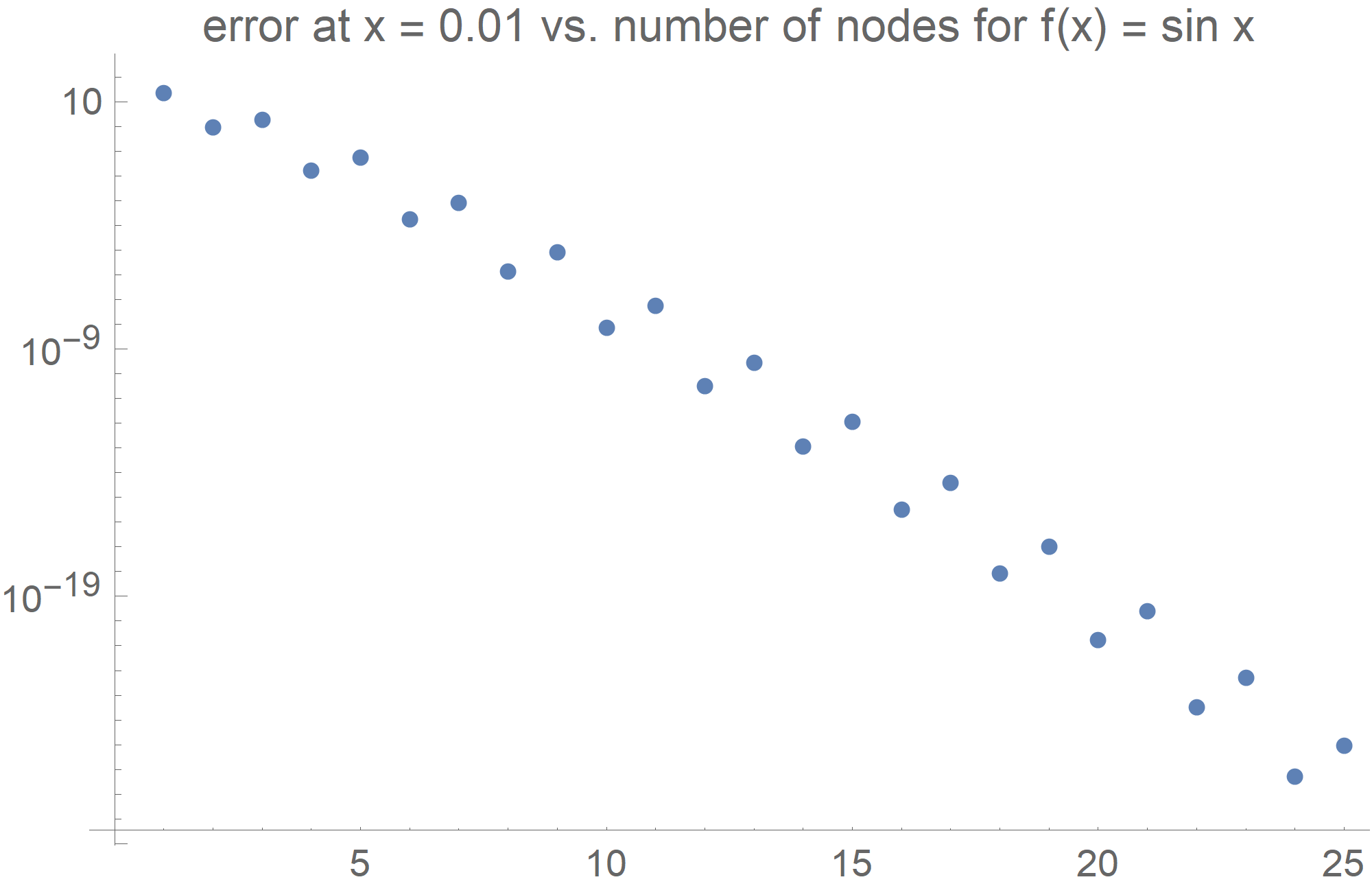
Figure 1. Absolute errors of $H_{w^{2}}[f;x]$ when computed by our algorithm vs. the number $n$ of nodes for $f(t)=\sin t$ and $x=0.01$.

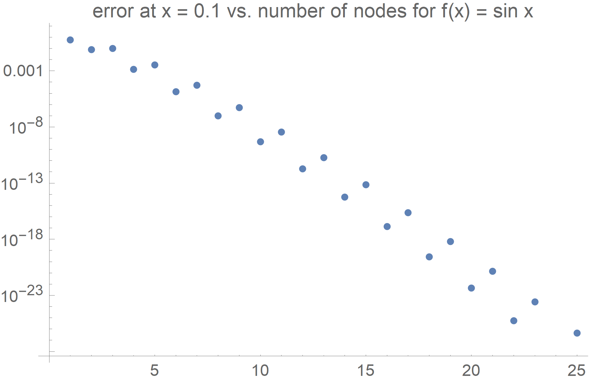
Figure 2. Absolute errors of $H_{w^{2}}[f;x]$ when computed by our algorithm vs. the number $n$ of nodes for $f(t)=\sin t$ and $x=0.1$.

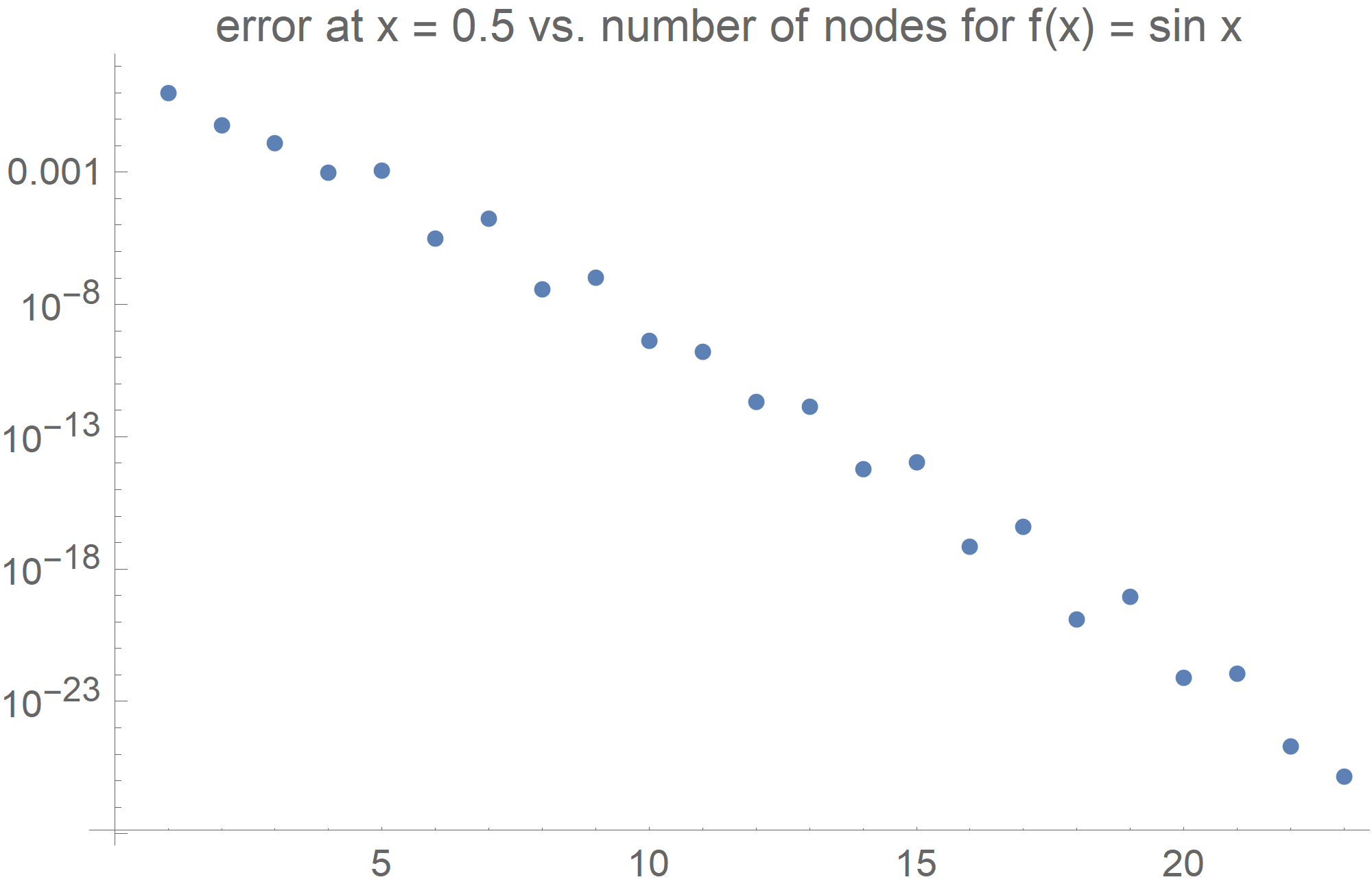
Figure 3. Absolute errors of $H_{w^{2}}[f;x]$ when computed by our algorithm vs. the number $n$ of nodes for $f(t)=\sin t$ and $x=0.5$.

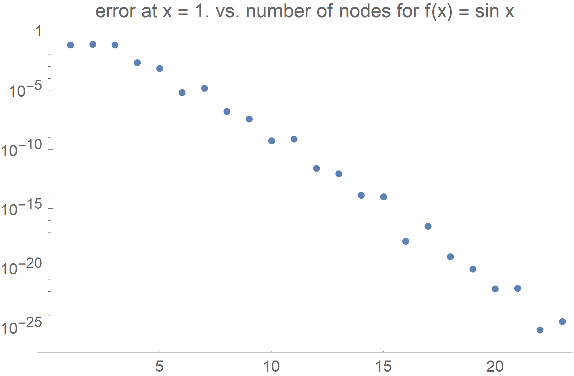
Figure 4. Absolute errors of $H_{w^{2}}[f;x]$ when computed by our algorithm vs. the number $n$ of nodes for $f(t)=\sin t$ and $x=1$.

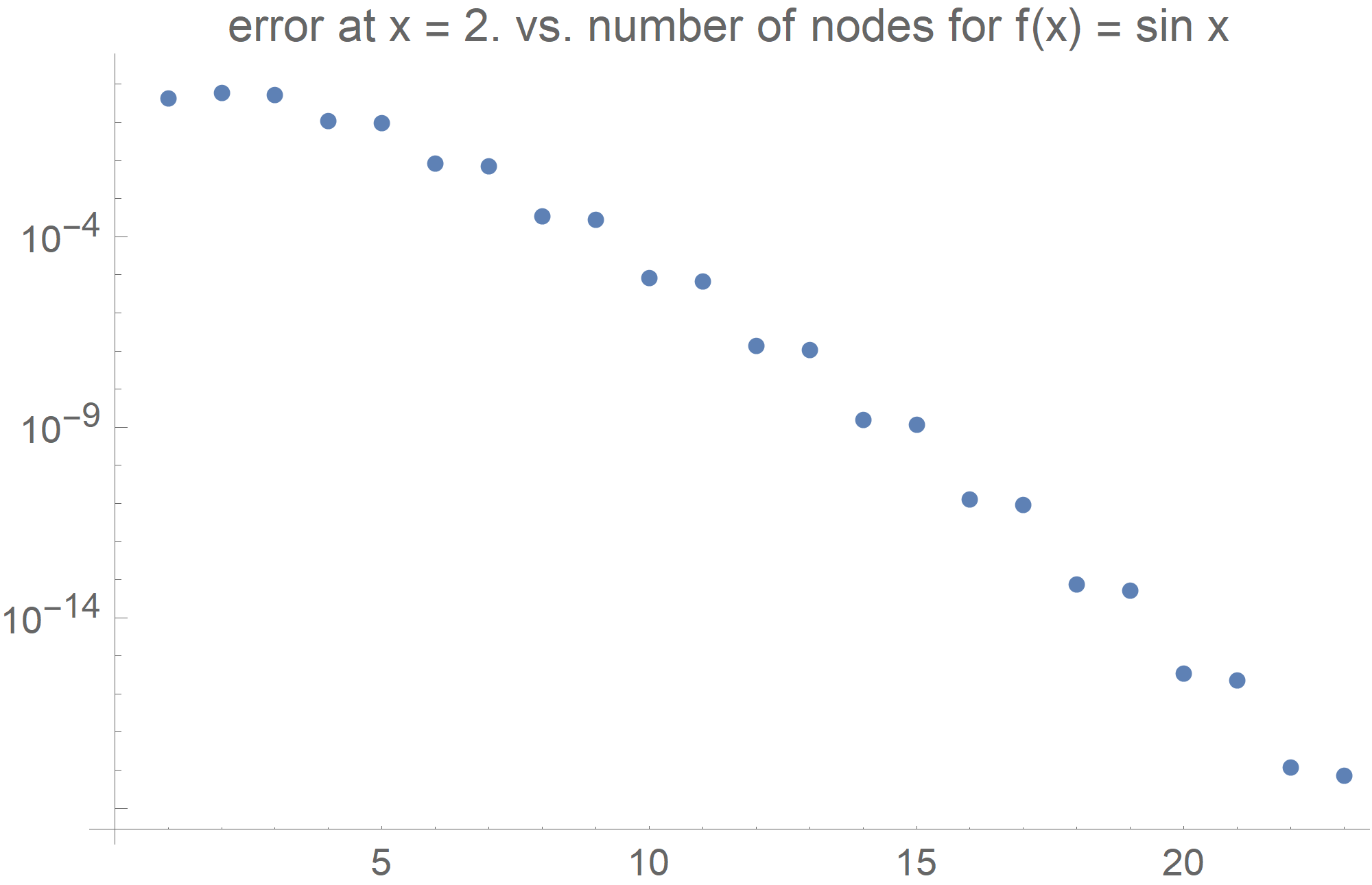
Figure 5. Absolute errors of $H_{w^{2}}[f;x]$ when computed by our algorithm vs. the number $n$ of nodes for $f(t)=\sin t$ and $x=2$.

Example 6.2.

The second example is very similar to the first one, the only change being that we now use the function $f(t)=\log(1+t^{2})$. For this example, we can observe the same very good convergence properties as in Example 6.1, see Figures 6–10.

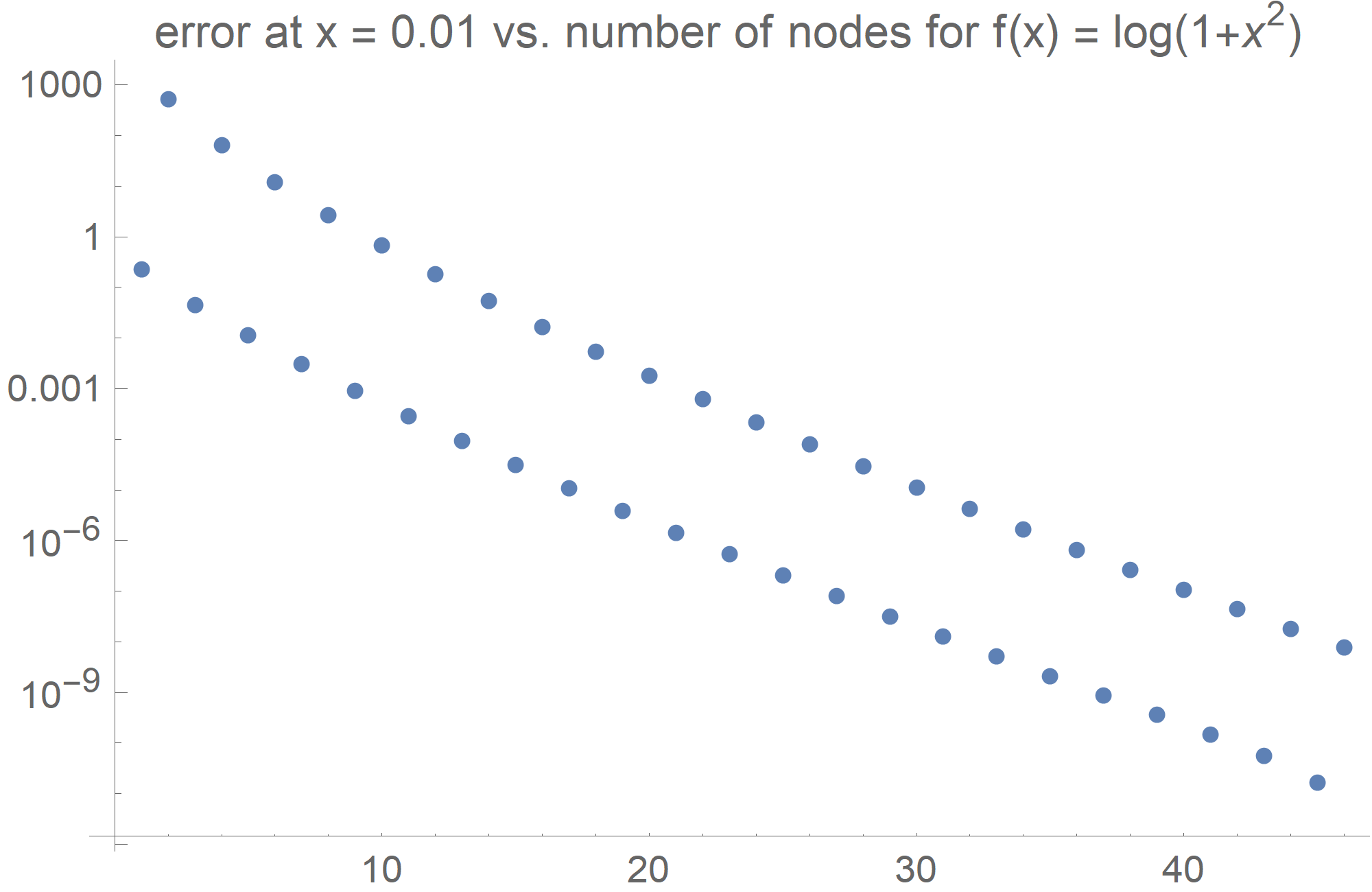
Figure 6. Absolute errors of $H_{w^{2}}[f;x]$ when computed by our algorithm vs. the number $n$ of nodes for $f(t)=\log(1+t^{2})$ and $x=0.01$.

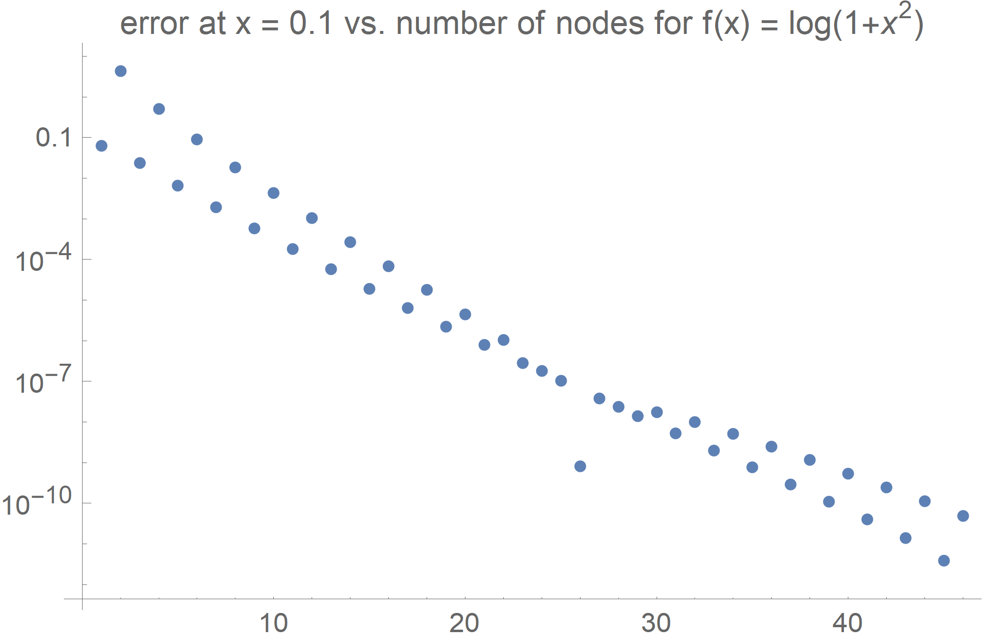
Figure 7. Absolute errors of $H_{w^{2}}[f;x]$ when computed by our algorithm vs. the number $n$ of nodes for $f(t)=\log(1+t^{2})$ and $x=0.1$.

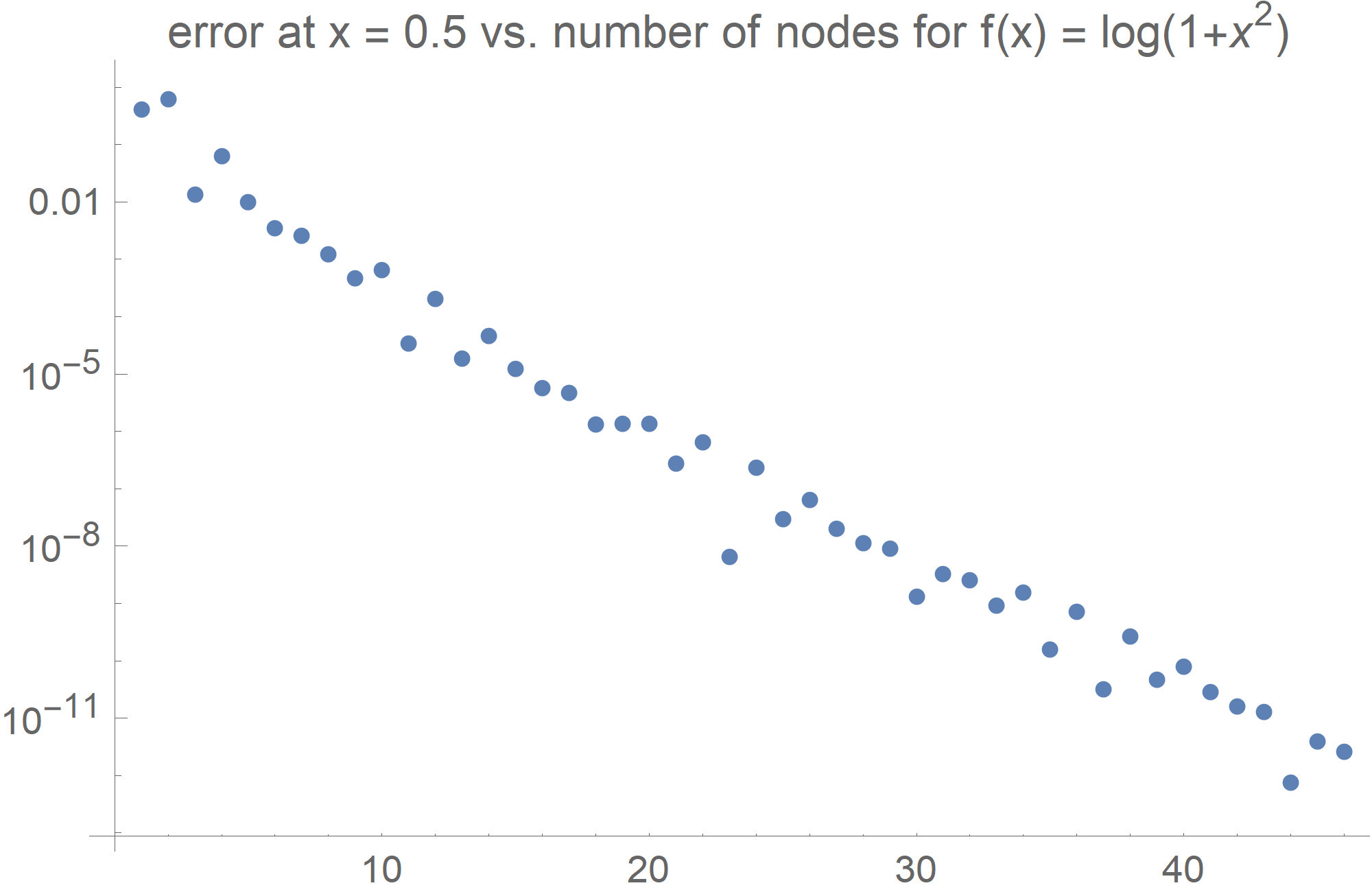
Figure 8. Absolute errors of $H_{w^{2}}[f;x]$ when computed by our algorithm vs. the number $n$ of nodes for $f(t)=\log(1+t^{2})$ and $x=0.5$.

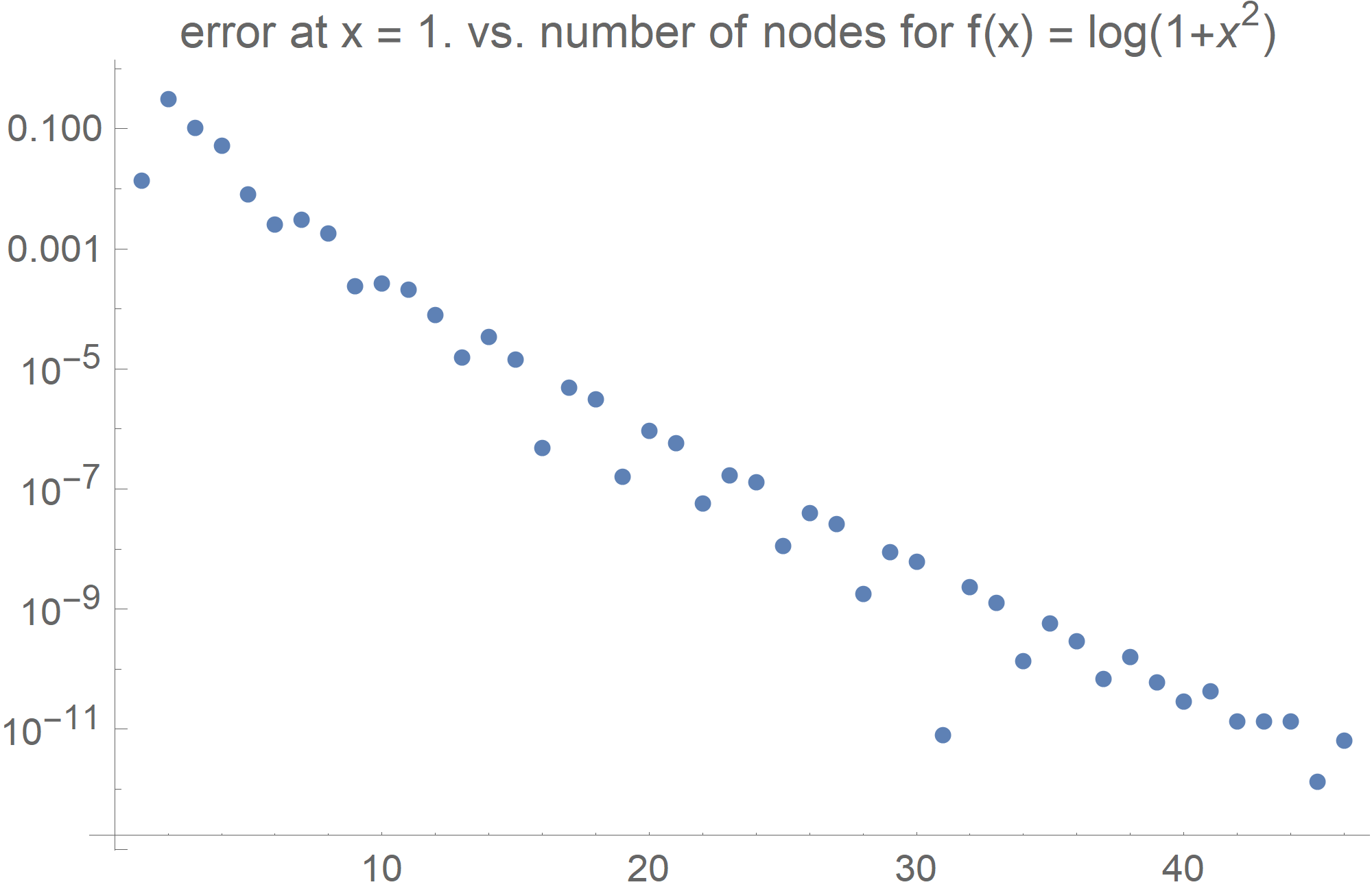
Figure 9. Absolute errors of $H_{w^{2}}[f;x]$ when computed by our algorithm vs. the number $n$ of nodes for $f(t)=\log(1+t^{2})$ and $x=1$.

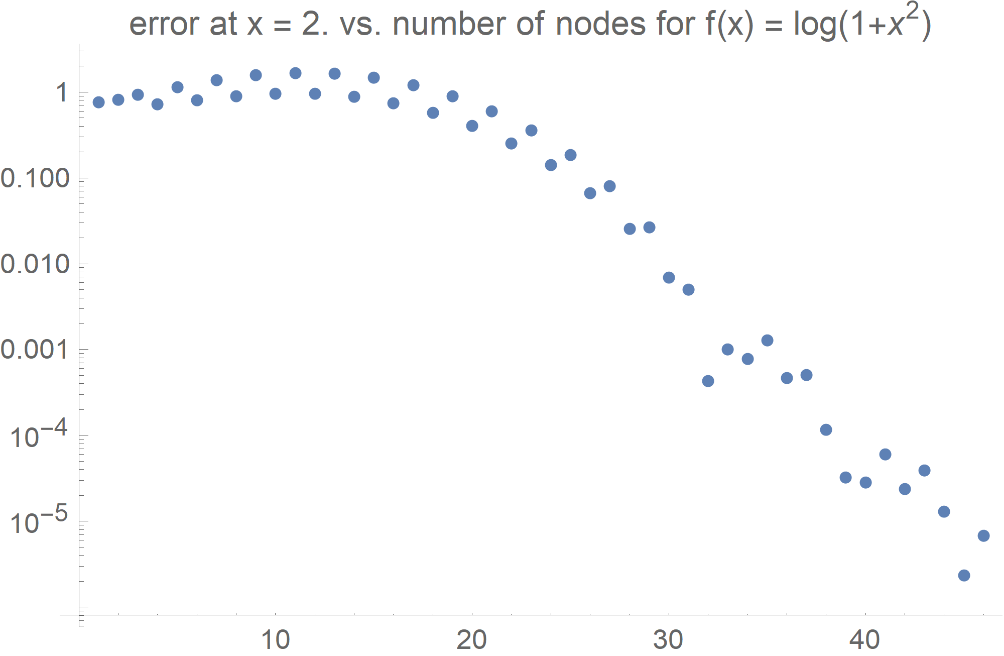
Figure 10. Absolute errors of $H_{w^{2}}[f;x]$ when computed by our algorithm vs. the number $n$ of nodes for $f(t)=\log(1+t^{2})$ and $x=2$.

Appendix A Some needed potential theoretical background

In order to understand the deep differences in the problems we consider in this paper to those studied in our papers [6, 7, 8, 9] and the complexities involved from moving from the results of [6, 7, 8, 9] to those in this paper, we believe it useful to add the following last section as an appendix. The fundamental weighted energy problem on the real line:

Let $\Sigma$ be a closed set on the real line and $w=\exp(-Q):\Sigma\to[0,\infty)$ be an upper semi-continuous weight function on $\Sigma$ with external field $Q$ that is positive on a set of positive linear Lebesgue measure. If $\Sigma$ is unbounded, we assume that

$$\lim_{|x|\to\infty,\,x\in\Sigma}(Q(x)-\log(x))=\infty.$$

Fix $\Sigma$ and $Q$ and consider

$${\rm inf}_{\mu}\left(\int\int\log\frac{1}{|x-t|}d\mu(x)d\mu(t)+2\int Qd\mu\right)$$

where the infimum is taken over all positive Borel measures $\mu$ with the support of $\mu$, ${\rm supp}(\mu)$ in $\Sigma$ and with $\mu(\Sigma)=1$. The infimum is attained by a unique minimizer $\mu_{w}$. Let

$$V^{\mu_{w}}(x)=\int\log\left(\frac{1}{|x-t|}\right)d\mu_{w}(t),\,x\in\mathbb{R}$$

be the logarithmic potential for $\mu_{w}$. Then the following variational inequalities hold:

(A.1) $$\begin{array}[]{ccc}V^{\mu_{w}}(x)+Q(x)\geq F_{w}&{\rm q.e.}&x\in\Sigma\\ V^{\mu_{w}}(x)+Q(x)=F_{w}&{\rm q.e.}&x\in{\rm supp}(\mu_{w})\end{array}$$

Here, $F_{w}$ is a constant and q.e. (quasi everywhere) means, with the exception of a set of logarithmic capacity zero.

The support of $\mu_{w}$ is one of the most important and fundamental quantities to determine the minimizer $\mu_{w}$, an extremely important and challenging problem which appears in diverse areas in mathematics and physics such as orthogonal polynomials, random matrix theory, combinatorics, approximation theory, electron configiurations on conductors, integrable systems, number theory and many more. When $Q$ is identically zero, the support of $\mu_{w}$ typically ”lives” close to the boundary of the set $\Sigma$ but when $Q$ is no longer identically zero, the support of $\mu_{w}$ depends heavily on $Q$ for example, its regularity and smoothness and can be quite arbitrary. The more complicated support of $\mu_{w}$ in the case of the work in this paper compared to the support of $\mu_{w}$ in our papers [6, 7, 8, 9], is one important reason why the research in the current paper differs from our previous work in [6, 7, 8, 9] so substantially.

A.1. The case $\Sigma=\mathbb{R}$ and one interval: $Q$ even.

The research on orthogonal polynomials, their zeroes and associated Christoffel functions, as used as critical tools in our papers [6, 7, 8, 9], was developed by Lubinsky and Levin [19]. In particular, if $Q$ is even, $Q^{\prime}$ exists in $(0,\infty)$ and $xQ^{\prime}$ increasing on $(0,\infty)$ and positive there, the support of $\mu_{w}$ is given in Remark 2.3.

A.2. The case $\Sigma=\mathbb{R}$ and one interval.

Here, Lubinsky and Levin in their classic monograph [19], established remarkable research on orthogonal polynomials, their zeroes and Christoffel functions to allow for the research in this paper. See Sections (2-5). In particular, under hypotheses on $Q$ such as given in Definition 2.1, the support of $\mu_{w}$ is given as in Definition 2.2.

A.3. The case $\Sigma=\mathbb{R}$

Deift and his collaborators in their papers [12, 13, 14] studied the support of $\mu_{w}$ for smooth $Q$, for example polynomials and obtained many term asymptotics for the associated orthogonal polynomials and their zeroes. We did not use their research in this paper and leave that for future work. In this case, the support of $\mu_{w}$ typically need not be one interval; indeed it often splits into a finite number of intervals (sometimes with gaps) with endpoints described often using tools such as Riemann Hilbert problems.

A.4. Some other cases.

Damelin, Benko, Dragnev, Kuijlaars, Deift, Olver [2, 10, 11, 26, 27] and many others have studied cases of $Q$ and $\Sigma$ where the support $\mu_{w}$ splits into a finite number of intervals (often with gaps) and with endpoints not necessarily known. Lubinsky and Levin have in recent years established remarkable results on asymptotics of orthogonal polynomials, their zeroes and Christoffel functions under very mild conditions on $Q$ and on various sets $\Sigma$. We do not use their research in this paper. See [20, 21].

In summary, descriptions of supports of minimizers for logarithmic energy variational problems such as (6.1) (and we do not discuss other kernels!) and associated research on their orthogonal polynomials, zeros and Christoffel functions for different $Q$ is a huge area of research in many areas of mathematics and physics. In particular, and in this regard, our results and methods in this paper, generalize, highly non-trivially our work in [6, 7, 8, 9].

Appendix B Comments on the Numerical Method

In this appendix we collect some information that is helpful in the construction and implementation of the numerical algorithm for the quadrature formula (3.2) required for the numerical examples presented in Section 6. To avoid excessive technical complications, the discussion here will not cover the very general weight functions investigated in the main part of the paper. Rather, we will restrict our attention to the special case discussed in Section 6, i.e. we shall assume throughout this appendix that $w$ is the Freud-type weight given by

(B.1) $$w(t)=\exp(-Q(t))\qquad\mbox{ with }\qquad Q(t)=t^{4}$$

for $t\in\mathbb{R}$. Furthermore, as indicated in Section 6, the algorithmic aspects are not the main point of this more theoretically oriented paper. Therefore, we emphasize here that the description below is also rather theoretical and does not include issues like the numerical stability of the approach. It is well known that this is a highly nontrivial matter that, however, needs to be discussed elsewhere.

The main observation in the present context is that, in view of eq. (3.3), the construction of the formula $Q_{n}[f;x]$ requires the following ingredients:

1. We need to be able to compute the Lagrange interpolation polynomial $L_{n}[f]$ for the given function $f$. In view of the well known general relation

   (B.2) $$L_{n}[f](t)=\sum_{j=1}^{n}f(x_{j,n})\prod_{\stackrel{{\scriptstyle\scriptstyle k=1}}{{k\neq j}}}^{n}\frac{t-x_{k,n}}{x_{j,n}-x_{k,n}},$$

   this means that we need to know the location of the nodes $x_{j,n}$ ($j=1,2,\ldots,n$), i.e. the zeros of the orthonormal polynomials $p_{n}=p_{n}(w^{2},\cdot)$ with respect to the weight function $w^{2}$.

2. In the second step, it is necessary to apply the weighted Hilbert transform operator $H_{w^{2}}$ to this interpolation polynomial. In view of the linearity of the Hilbert transform, this demands the knowledge of the values of $H_{w^{2}}[\pi_{k};x]$ for $k=0,1,2,\ldots,n$ where $\pi_{k}(t)=t^{k}$ is the $k$th monomial.

We shall now describe how this information can be obtained.

B.1. The moments of the weight function $w^{2}$

It turns out that, for both required items, it is necessary to compute the moments

(B.3) $$\mu_{k}:=\int_{-\infty}^{\infty}w^{2}(t)t^{k}dt$$

of the given weight function $w^{2}$ for $k=0,1,2,\ldots,2n$, so this is our first result. Indeed, we can see that

(B.4) $$\mu_{k}=\begin{cases}0&\mbox{ if }k\mbox{ is odd,}\\ 2^{-(k+5)/4}\cdot\Gamma\left(\frac{k+1}{4}\right)&\mbox{ if }k\mbox{ is even,}\end{cases}$$

where $\Gamma$ denotes Euler’s Gamma function. The result for odd values of $k$ immediately follows from a symmetry argument because the weight function $w^{2}$ is even, and the result for even values of $k$ can be obtained by a symbolic integration using a computer algebra package like Mathematica [29].

B.2. The nodes of the interpolation operator $L_{n}$

As indicated above, the nodes of the interpolation operator $L_{n}$ are the zeros of the orthonormal polynomial $p_{n}(w^{2},\cdot)$. To determine these values, we follow a strategy outlined in [17]. Specifically, we consider the orthogonal polynomials $\tilde{p}_{n}(w^{2},\cdot)$ for the weight function $w^{2}$ that, instead of being normalized according to (3.1), are normalized such that their leading coefficient is 1. Clearly, this means that, for each $n$, there exists some real number $C_{n}$ such $p_{n}(w^{2},x)=C_{n}\tilde{p}_{n}(w^{2},x)$ holds for all $x\in\mathbb{R}$, and hence the zeros of $p_{n}(w^{2},\cdot)$ coincide with those of $\tilde{p}_{n}(w^{2},\cdot)$. It is then a well known general property of orthogonal polynomials that there exist real numbers $\alpha_{k},\beta_{k}$ ($k=0,1,2,\ldots$) depending on the weight function $w^{2}$ such that the polynomials $\tilde{p}_{n}(w^{2},\cdot)$ satisfy the three-term recurrence relation

(B.5a) $$\tilde{p}_{k+1}(w^{2},t)=(t-\alpha_{k})\tilde{p}_{k}(w^{2},t)-\beta_{k}\tilde{p}_{k-1}(w^{2},t)\qquad k=0,1,2,\ldots$$

with starting values

(B.5b) $$\tilde{p}_{0}(w^{2},t)=1\qquad\mbox{ and }\qquad\tilde{p}_{-1}(w^{2},t)=0,$$

cf., e.g., [17, eq. (1.3)]. From [17, Section 6.1] we can then conclude that the desired zeros of the polynomial $\tilde{p}_{n}(w^{2},\cdot)$ (and hence also the zeros of $p_{n}(w^{2},\cdot)$, i.e. the required interpolation nodes) are the eigenvalues of the tridiagonal matrix

$$M_{n}=\begin{pmatrix}\alpha_{0}&\sqrt{\beta_{1}}&&&&\\ \sqrt{\beta_{1}}&\alpha_{1}&\sqrt{\beta_{2}}&&&\\ &\ddots&\ddots&\ddots&\\ &&\sqrt{\beta_{n-2}}&\alpha_{n-2}&\sqrt{\beta_{n-1}}\\ &&&\sqrt{\beta_{n-1}}&\alpha_{n-1}\end{pmatrix}.$$

So, to compute the interpolation nodes, we have to find the entries of the matrix $M_{n}$ and then calculate its eigenvalues.

For the former step, we must determine the values $\alpha_{k}$ and $\beta_{k}$. To this end, we first note that, in our case,

$$\alpha_{k}=0\qquad\mbox{ for all }k;$$

this follows because the weight function $w^{2}$ that we have chosen is even. For the $\beta_{k}$, we use the bootstrap method (also known as the Stieltjes procedure) described in [17, Section 4.1] that can be formulated in the following way:

• Set $\beta_{0}=\int_{-\infty}^{\infty}w^{2}(t)dt=\mu_{0}$ (which is known from eq. (B.4)).

• For $k=0,1,2,\ldots,n-1$:

  • Compute $\tilde{p}_{k+1}(w^{2},\cdot)$ by means of eq. (B.5a).

  • Compute

    (B.6) $$\beta_{k+1}=\frac{\int_{-\infty}^{\infty}w^{2}(t)\left(\tilde{p}_{k+1}(w^{2},t)\right)^{2}dt}{\int_{-\infty}^{\infty}w^{2}(t)\left(\tilde{p}_{k}(w^{2},t)\right)^{2}dt}.$$

Note that the computation of the integrals in eq. (B.6) is technically possible because the coefficients of the polynomials $p_{\ell}(w^{2},\cdot)$ ($\ell=k,k+1$) in the integrands have already been computed, so the squares of these polynomials can be computed as well, and therefore these integrals can be expressed as linear combinations of the known moments $\mu_{\ell}$ with known coefficients.

It then remains to compute the eigenvalues of $M_{n}$. In view of the tridiagonal structure of $M_{n}$, this is a straightforward process in numerical linear algebra; the QR method, for example, is a reliable, stable and efficient method to accomplish this goal.

B.3. Evaluation of $H_{w^{2}}[L_{n};x]$

We now have all the components of the right-hand side of eq. (B.2) available, and so we can compute the interpolation polynomial $L_{n}[f]$ and express it in the canonical form

$$L_{n}[f](t)=\sum_{k=0}^{n-1}\lambda_{kn}[f]t^{k}$$

with certain coefficients $\lambda_{kn}[f]$ that depend on the given function $f$. It then follows that

$$H_{w^{2}}[L_{n};x]=-\!\!\!\!\!\!\!\!\;\int_{-\infty}^{\infty}w^{2}(t)\frac{L_{n}[f](t)}{t-x}dt=J_{1}[f](x)+L_{n}[f](x)J_{2}(x)$$

where

$$J_{1}[f](x)=\int_{-\infty}^{\infty}w^{2}(t)\frac{L_{n}[f](t)-L_{n}[f](x)}{t-x}dt$$

and

$$J_{2}(x)=-\!\!\!\!\!\!\!\!\;\int_{-\infty}^{\infty}w^{2}(t)\frac{1}{t-x}dt.$$

For $J_{1}[f](x)$, we see for any $x\in\mathbb{R}$ that

$$J_{1}[f](x) = \int_{-\infty}^{\infty}w^{2}(t)\frac{\sum_{k=0}^{n-1}\lambda_{kn}[f]t^{k}-\sum_{k=0}^{n-1}\lambda_{kn}[f]x^{k}}{t-x}dt$$

$$= \int_{-\infty}^{\infty}w^{2}(t)\sum_{k=1}^{n-1}\lambda_{kn}[f]\frac{t^{k}-x^{k}}{t-x}dt$$

$$= \int_{-\infty}^{\infty}w^{2}(t)\sum_{k=1}^{n-1}\lambda_{kn}[f]\sum_{\ell=0}^{k-1}t^{\ell}x^{k-\ell-1}dt$$

$$= \sum_{k=1}^{n-1}\lambda_{kn}[f]\sum_{\ell=0}^{k-1}x^{k-\ell-1}\mu_{\ell}$$

which can be evaluated with the help of eq. (B.4).

For the integral $J_{2}(x)$, we first note that, owing to the fact that $w^{2}$ is an even function, $J_{2}$ is an odd function. Therefore, $J_{2}(0)=0$ and $J_{2}(x)=-J_{2}(-x)$ for all $x<0$. Hence it suffices to explicitly consider the computation of $J_{2}(x)$ for $x>0$; the remaining cases can be covered by symmetry arguments. In this case we can use the fact that our specific application uses $w^{2}(t)=\exp(-2t^{4})$, cf. eq. (B.1), and argue as follows:

$$J_{2}(x)=\int_{-\infty}^{0}\frac{\exp(-2t^{4})}{t-x}dt+-\!\!\!\!\!\!\!\!\;\int_{0}^{\infty}\frac{\exp(-2t^{4})}{t-x}dt=J_{21}(x)+J_{22}(x),$$

say, where (using the substitution $t=-u^{1/4}$ in the first step and the symbolic integration capabilities of Mathematica [29] in the last one)

$$J_{21}(x) = \int_{-\infty}^{0}\frac{\exp(-2t^{4})}{t-x}dt$$

$$= \frac{1}{4}\int_{0}^{\infty}\frac{\exp(-2u)}{-u-xu^{3/4}}du$$

$$= \frac{1}{4}\int_{0}^{\infty}\exp(-2u)\left[\frac{1}{x^{3}u^{1/4}}-\frac{1}{x^{2}u^{1/2}}+\frac{1}{xu^{3/4}}-\frac{1}{x^{3}(x+u^{1/4})}\right]du$$

$$= \frac{\Gamma(3/4)}{2^{11/4}x^{3}}+\frac{\Gamma(1/4)}{2^{9/4}x}$$

$${}+\exp(-2x^{4})\Bigg{[}\frac{\pi\mathrm{i}}{4}\mathop{\mathrm{erf}}(\mathrm{i}\sqrt{2}x^{2})-\frac{1}{4}\mathop{\mathrm{Ei}}(2x^{4})-\frac{\pi\mathrm{i}}{2}$$

$$\phantom{\exp(-2x^{4})\Bigg{]}abc}{}+\frac{3\sqrt{2}}{128}(-1+\mathrm{i})\Gamma\left(-\frac{1}{4}\right)\Gamma\left(-\frac{3}{4},-2x^{4}\right)$$

$$\phantom{\exp(-2x^{4})\Bigg{]}abc}{}-\frac{\sqrt{2}}{8}(1+\mathrm{i})\Gamma\left(\frac{5}{4}\right)\Gamma\left(-\frac{1}{4},-2x^{4}\right)\Bigg{]}.$$

In this formula, $\mathrm{i}$ is the imaginary unit, $\mathop{\mathrm{erf}}$ denotes the error function, $\mathop{\mathrm{Ei}}$ is the exponential integral, and $\Gamma(\cdot,\cdot)$ is the incomplete Gamma function. Note that, as one may expect since $J_{21}(x)$ is the integral of a real valued function over a real interval, all the imaginary parts of the components of the final expression for $J_{21}(x)$ cancel each other, and so the result is purely real.

Finally, using the substitution $t=u^{1/4}$ in the first step and once again the symbolic integration capabilities of Mathematica in the last one, we find

$$J_{22}(x)\!\!\!\!\! = \!\!\!\!\!-\!\!\!\!\!\!\!\!\;\int_{0}^{\infty}\frac{\exp(-2t^{4})}{t-x}dt$$

$$= \!\!\!\!\!\frac{1}{4}-\!\!\!\!\!\!\!\!\;\int_{0}^{\infty}\frac{\exp(-2u)}{u-xu^{3/4}}du$$

$$= \!\!\!\!\!\frac{1}{4}-\!\!\!\!\!\!\!\!\;\int_{0}^{\infty}\exp(-2u)\left[-\frac{1}{x^{3}u^{1/4}}-\frac{1}{x^{2}u^{1/2}}-\frac{1}{xu^{3/4}}+\frac{1}{x^{3}(u^{1/4}-x)}\right]du$$

$$= \!\!\!\!\!-\frac{\sqrt{2}\pi}{8x^{2}}-\frac{\Gamma(\nicefrac{{3}}{{4}})}{2^{11/4}x^{3}}-\frac{\Gamma(\nicefrac{{1}}{{4}})}{2^{9/4}x}-\frac{\pi}{2x^{4}}G_{8,9}^{5,4}\!\left(\!\begin{matrix}\nicefrac{{1}}{{4}},\nicefrac{{1}}{{2}},\nicefrac{{3}}{{4}},1,\nicefrac{{1}}{{8}},\nicefrac{{3}}{{8}},\nicefrac{{5}}{{8}},\nicefrac{{7}}{{8}}\\ \nicefrac{{1}}{{4}},\nicefrac{{1}}{{2}},\nicefrac{{3}}{{4}},1,1,\nicefrac{{1}}{{8}},\nicefrac{{3}}{{8}},\nicefrac{{5}}{{8}},\nicefrac{{7}}{{8}}\end{matrix}\,\Bigg{|}\,2x^{4}\!\!\right)$$

where $G_{8,9}^{5,4}$ is a member of the class of Meijer’s $G$-functions (see, e.g., [1]).

Combining all the results listed in Appendix B, we can implement the algorithm used for computing the numerical results of Section 6.

Declaration of interest statement

The authors report there are no competing interests to declare.

References

- [1] R. Beals and J. Szmigielski, Meijer –functions: A gentle introduction, Notices Am. Math. Soc., 60 (2013), 866–872.
- [2] D. Benko, S. B. Damelin and P. Dragnev, On the support of the equilibrium measure for arcs of the unit circle and real intervals, Electron. Trans. Numer. Anal., 25 (2006), 27–40.
- [3] G. Criscuolo, B. Della Vecchia, D. S. Lubinsky and G. Mastroianni, Functions of the second kind for Freud weights and series expansions of Hilbert transforms, J. Math. Anal. Appl., 189 (1995), 256–296.
- [4] G. Criscuolo and G. Mastroianni, On the convergence of an interpolatory product rule for evaluating Cauchy principal value integrals, Math. Comput., 48 (1987), 725–735.
- [5] S. B. Damelin, On the maximum modulus of weighted polynomials in the plane, a theorem of Rakhmanov, Mhaskar and Saff revisited, J. Comput. Appl. Math., 155 (2003), 455–459.
- [6] S. B. Damelin and K. Diethelm, Interpolatory product quadratures for Cauchy principal value integrals with Freud weights, Numer. Math., 83 (1999), 87–105.
- [7] S. B. Damelin and K. Diethelm, Boundedness and uniform numerical approximation of the weighted Hilbert transform on the real line, Numer. Funct. Anal. Optim., 22 (2001), 13–54.
- [8] S. B. Damelin and K. Diethelm, Numerical approximation and stability of singular integral equations for Freud exponential weights on the line, J. Integral Equations Appl., 16 (2004), 273–292.
- [9] S. B. Damelin and K. Diethelm, Weighted polynomial approximation and Hilbert transforms: Their connections to the numerical solution of singular integral equations, in Proceedings of the 4th International Conference on Dynamic Systems and Applications. Dynamic Publishers, Atlanta (2004), 20–26.
- [10] S. B. Damelin, P. Dragnev and A. Kuijlaars, The support of the equilibrium measure for a class of external fields on a finite interval, Pac. J. Math., 199 (2001), 303–321.
- [11] S. B. Damelin and A. Kuijlaars, The support of the extremal measure for monomial external fields on , Trans. Amer. Math. Soc., 351 (1999), 4561–4584.
- [12] P. Deift, Orthogonal Polynomials and Random Matrices: A Riemann-Hilbert Approach, Amer. Math. Soc., Providence, 2000.
- [13] P. Deift, T. Kriecherbauer, K. T.-R. McLaughlin, S. Venakides and X. Zhou, Strong asymptotics of orthogonal polynomials with respect to exponential weights, Commun. Pure Appl. Math., 52 (1999), 1491–1552.
- [14] P. Deift, T. Kriecherbauer, K. T.-R. McLaughlin, S. Venakides and X. Zhou, Strong asymptotics of orthogonal polynomials with respect to varying exponential weights and applications to universality questions in random matrix theory, Comm. Pure Appl. Math., 52 (1999), 1335–1425.
- [15] K. Diethelm, Gaussian quadrature formulae of the third kind for Cauchy principal value integrals: Basic properties and error estimates, J. Comput. Appl. Math., 65 (1995), 97–114.
- [16] K. Diethelm, The order of convergence of modified interpolatory quadratures for singular integrals of Cauchy type, Z. Angew. Math. Mech., 75 (1995), S621–S622.
- [17] W. Gautschi, Algorithm 726: ORTHPOL — A package of routines for generating orthogonal polynomials and Gauss-type quadrature rules, ACM Trans. Math. Software, 20 (1994), 21–62.
- [18] A. I. Kalandiya, Mathematical Methods of Two Dimensional Elasticity, 1st english ed., Mir, Moscow, 1975.
- [19] E. Levin and D. S. Lubinsky, Orthogonal Polynomials for Exponential Weights, Springer, New York, 2001.
- [20] E. Levin and D. S. Lubinsky, Bounds and Asymptotics for Orthgonal Polynomials for Varying Weights, Springer, Berlin, 2018.
- [21] E. Levin and D. S. Lubinsky, Asymptotics of orthogonal polynomials and separation of their zeros, to appear in Journal of Approximation Theory.
- [22] D. S. Lubinsky, A survey of weighted polynomial approximation with exponential weights, Surv. Approx. Theory, 3 (2007), 1–105.
- [23] D. S. Lubinsky and D. M. Matjila, Full quadrature sums for th powers of polynomials with Freud weights, J. Comput. Appl. Math., 60 (1995), 285–296.
- [24] H. N. Mhaskar, Introduction to the Theory of Weighted Polynomial Approximation, World Scientific, Singapore, 1996.
- [25] G. Monegato, On the weights of certain quadratures for the numerical evaluation of Cauchy principal value integrals and their derivatives, Numer. Math. 50 (1987), 273–281.
- [26] S. Olver, Computation of equilibrium measures, J. Approx. Theory, 163 (2011), 1185–1207.
- [27] S. Olver, A general framework for solving Riemann–Hilbert problems numerically, Numer. Math., 122 (2012), 305–340.
- [28] W. E. Smith, I. H. Sloan and A. H. Opie, Product integration over infinite intervals I: Rules based on the zeros of Hermite polynomials, Math. Comput. 40 (1983), 519–535.
- [29] Wolfram Research, Mathematica, Version 12.0. https://www.wolfram.com/mathematica/ Champaign, 2019.