Hyperfine structure of ${}^{2}\Sigma$ molecules containing alkaline-earth atoms

Jesus Aldegunde Departamento de Quimica Fisica, Universidad de Salamanca, 37008 Salamanca, Spain Jeremy M. Hutson J.M.Hutson@durham.ac.uk Joint Quantum Centre (JQC) Durham-Newcastle, Department of Chemistry, Durham University, South Road, Durham, DH1 3LE, United Kingdom

Abstract

Ultracold molecules with both electron spin and an electric dipole moment offer new possibilities in quantum science. We use density-functional theory to calculate hyperfine coupling constants for a selection of molecules important in this area, including RbSr, LiYb, RbYb, CaF and SrF. We find substantial hyperfine coupling constants for the fermionic isotopes of the alkaline-earth and Yb atoms. We discuss the hyperfine level patterns and Zeeman splittings expected for these molecules. The results will be important both to experiments aimed at forming ultracold open-shell molecules and to their applications.

pacs:

33.15.Fm,42.62.Eh,37.10.Mn

There have recently been major advances in producing molecules in ultracold gases of alkali-metal atoms. Ultracold molecules have been produced from most combinations of alkali-metal atoms by magnetoassociation, in which pairs of atoms are converted into molecules by tuning a magnetic field adiabatically across a zero-energy Feshbach resonance. These “Feshbach molecules” are typically bound by less than $h\times 10$ MHz, which is less than part in $10^{7}$ of the singlet well depth, and have very large internuclear separations. A few different molecules (⁴⁰K⁸⁷Rb Ni et al. (2008), ⁸⁷Rb¹³³Cs Takekoshi et al. (2014); Molony et al. (2014), ²³Na⁴⁰K Park et al. (2015) and ²³Na⁸⁷Rb Guo et al. (2016)) have recently been transfered from these long-range states to the absolute ground state by Stimulated Raman Adiabatic Passage (STIRAP). These ground-state molecules have significant electric dipole moments, and hold great promise for studying ultracold dipolar matter, for precision measurement, and for applications in quantum science and technology.

The alkali-metal dimers all have singlet ground states, with no net electron spin. This limits their tunability with magnetic fields. There is now great interest in producing ultracold molecules with electron spin as well as an electric dipole. Such molecules could be used to create new types of quantum many-body systems Micheli et al. (2006); Baranov et al. (2012). Promising candidates include molecules formed from an alkali-metal atom and a laser-coolable closed-shell atom such as Yb or Sr. Żuchowski et al. Żuchowski et al. (2010) showed that magnetically tunable Feshbach resonances can exist in such systems, mediated by the dependence of the alkali-metal hyperfine coupling on the internuclear distance. Brue and Hutson Brue and Hutson (2013) carried out a detailed theoretical study of such resonances in alkali metal + Yb systems. Brue and Hutson Brue and Hutson (2012) also identified a different mechanism that can cause additional resonances in systems containing closed-shell atoms with nuclear spin (which are all fermionic for Sr and Yb), mediated in this case by hyperfine coupling involving the Sr or Yb nucleus. The first Feshbach resonances of both these types have recently been observed in RbSr Barbé et al. (2017), along with resonances due to another mechanism involving the tensorial coupling between the electron and nuclear spins. It is likely that ultracold ground-state ${}^{2}\Sigma$ molecules of this type will be produced within the next few years.

In parallel with the work on producing ultracold molecules from atoms, there have been major advances in direct laser-cooling of molecules such as CaF and SrF, which also have ${}^{2}\Sigma$ ground states. Barry et al. Barry et al. (2014) have cooled SrF to about 2.5 mK in a magneto-optical trap (MOT), and Truppe et al. Truppe et al. (2017) have achieved sub-Doppler cooling of CaF in a blue-detuned MOT to about 50 $\mu$ K.

Although the basic spectroscopy of molecules in ${}^{2}\Sigma$ states is well understood Brown and Carrington (2003), little is known quantitatively about the fine and hyperfine coupling constants of molecules formed from alkali-metal atoms and closed-shell atoms, or about isotopologs of CaF and SrF containing metal atoms with non-zero spin. The magnitudes of the coupling constants will have profound effects on the patterns of energy levels for ground-state molecules, and how the levels cross and avoided-cross one another in magnetic, electric and laser fields. This will in turn affect the possibilities for state transfer and quantum control. The coupling constants are also important to understand the strengths of Feshbach resonances Żuchowski et al. (2010); Brue and Hutson (2012, 2013); Barbé et al. (2017). In this paper we present calculations of the fine and hyperfine constants for RbSr, LiYb, RbYb, CaF and SrF, using density-functional theory, which allow these effects to be explored.

I Molecular Hamiltonian

The effective hamiltonian for a ${}^{2}\Sigma$ diatomic molecule can be written

H_{\rm{eff}}=H_{\rm{rfs}}+H_{\rm{hfs}}+H_{\rm{S}}+H_{\rm{Z}},

(1)

where the four contributions correspond to the rotational plus fine-structure, hyperfine, Stark and Zeeman Hamiltonians respectively.

The rotational plus fine-structure Hamiltonian $H_{\rm{rfs}}$ takes the standard form,

H_{\rm{rfs}}=B_{v}{\bm{N}}^{2}-D_{v}{\bm{N}}^{2}{\bm{N}}^{2}+\gamma{\bm{S}}\cdot{\bm{N}},

(2)

where $\bm{N}$ is the angular momentum for rotation of the molecule about its center of mass and $\bm{S}$ is the electron spin. The third term in Eq. 2 represents the electron spin-rotation interaction. The hyperfine hamiltonian $H_{\rm{hfs}}$ may be written

\displaystyle H_{\rm{hfs}}

\displaystyle=

\displaystyle\sum_{i=1}^{2}e{\bm{Q}}_{i}\cdot{\bm{q}}_{i}+\sum_{i=1}^{2}{\bm{S}}\cdot{\bm{A}}_{i}\cdot{\bm{I}}_{i},

(3)

where $\bm{I}_{1}$ and $\bm{I}_{2}$ are the spins of nuclei 1 and 2. The first term here represents the interaction between the quadrupole tensor $e\bm{Q}_{i}$ of nucleus $i$ and the electric field gradient tensor ${\bm{q}}_{i}$ at the nucleus due to the electrons; it is commonly written in terms of a scalar nuclear quadrupole coupling constant $(eQq)_{i}$ . The second term represents the interaction between the electron and nuclear spins. It is usual to separate the isotropic and anisotropic components of the hyperfine tensor ${\bm{A}}_{i}$ Kaupp et al. (2004),

b_{\rm{F}}=A_{\rm{iso}}=\frac{A_{\|}+2A_{\bot}}{3}\mbox{ and }t=A_{\rm{dip}}=\frac{A_{\|}-A_{\bot}}{3},

(4)

so that

{\bm{S}}\cdot{\bm{A}}_{i}\cdot{\bm{I}}_{i}=b_{{\rm F},i}{\bm{S}}\cdot{\bm{I}}_{i}+t_{i}\,\sqrt{6}\,T^{2}(\bm{S},\bm{I}_{i})\cdot T^{2}(C),

(5)

where $T^{2}$ indicates a spherical tensor of rank 2. $T^{2}(C)$ has components $C^{2}_{q}(\theta,\phi)$ , where $C$ is a renormalised spherical harmonic and $\theta,\phi$ are the polar coordinates of the internuclear vector. The isotropic (scalar) component $b_{{\rm F},i}$ arises from the Fermi contact interaction, whereas the anisotropic component $t_{i}$ arises from dipolar interactions. The notation involving $\gamma$ , $(eQq)_{i}$ , $b_{{\rm F},i}$ and $t_{i}$ coincides with that employed by Brown and Carrington Brown and Carrington (2003) (see, for example, page 607), where explicit expressions for the matrix elements in different basis sets can be found. The alternative constants of Frosch and Foley Frosch and Foley (1952) are related to these by $c_{i}=3t_{i}$ and $b_{i}=b_{{\rm F},i}-t_{i}.$

The effect of the external fields is described by $H_{\rm{S}}$ and $H_{\rm{Z}}$ , which represent the Stark and Zeeman Hamiltonians. The Stark Hamiltonian is

H_{\rm{S}}=-\bm{\mu}\cdot\bm{E}-\frac{1}{2}\bm{E}\cdot\bm{\alpha}\cdot\bm{E}.

(6)

It includes both a linear term to describe the interaction of the molecular dipole $\bm{\mu}$ with a static electric field $\bm{E}$ and a quadratic term involving the molecular polarizability tensor $\bm{\alpha}$ . The latter is usually small for static fields, but may be used with a frequency-dependent polarizability $\bm{\alpha}(\omega)$ to account for the ac Stark effect due to a non-resonant laser field Gregory et al. (2017). The Zeeman Hamiltonian is

	$\displaystyle H_{\rm{Z}}$	$\displaystyle=$	$\displaystyle-g_{\parallel}\mu_{\rm B}\bm{S}\cdot\bm{B}+\Delta g_{\bot}\mu_{\mathrm{B}}\left[\bm{S}\cdot\bm{B}-(\bm{S}\cdot\hat{z})(\bm{B}\cdot\hat{z})\right]$		(7)
			$\displaystyle-g_{\rm r}\mu_{\rm B}\bm{N}\cdot\bm{B}-\sum_{i=1}^{2}g_{i}\mu_{\rm N}\,\bm{I}_{i}\cdot\bm{B}(1-\sigma_{i}).$		(7)

The first term describes the isotropic part of the interaction of the electron spin with an external magnetic field $\bm{B}$ ; $g_{\parallel}\approx g_{e}\approx-2.0023$ is the electron g-factor parallel to the molecular axis $\hat{z}$ and $\mu_{\rm B}$ is the Bohr magneton. The second term is an anisotropic correction; $\Delta g_{\bot}=g_{\parallel}-g_{\bot}$ , where $g_{\bot}$ is the electron $g$ -factor perpendicular to the molecular axis (defined to be negative, like $g_{e}$ ). The third and fourth terms describe the interaction of the molecular rotation and the nuclear spins with the magnetic field; $g_{\rm r}$ is the rotational g-factor, and $g_{i}$ and $\sigma_{i}$ are the bare nuclear g-factor and shielding factor for nucleus $i$ . $\mu_{\rm N}$ is the nuclear magneton. The Zeeman Hamiltonian $H_{\rm{Z}}$ is dominated by the first term, but the remaining contributions cause small shifts that may have important consequences for resonance positions Barbé et al. (2017) and for the decoherence of molecules in magnetic traps Blackmore et al. (2018).

The expressions given above neglect various small terms such as the interactions between the two nuclear spins and between the nuclear spins and molecular rotation. These terms can be important for closed-shell molecules Aldegunde et al. (2008); Aldegunde and Hutson (2009); Aldegunde et al. (2009); Aldegunde and Hutson (2017), but for open-shell molecules they are less important because the terms involving electron spin are always present and are two or more orders of magnitude larger. A full description of the Hamiltonian, including the discarded terms, can be found in Ref. Brown and Carrington (2003).

II Calculation of the coupling constants

Molecular fine-structure and hyperfine constants may in principle be calculated using either wavefunction-based methods or density-functional theory (DFT). However, wavefunction-based methods become very complex for hyperfine interactions in molecules containing heavy atoms, where very large basis sets are needed and relativistic effects are important. Calculations of potential curves for such molecules commonly use effective core potentials, but these are of doubtful accuracy for hyperfine interactions. We therefore choose to use DFT in the current work, and obtain values of the coupling constants $(eQq)$ , $b_{\rm{F}}$ , $t$ and $\Delta g_{\bot}$ using the Amsterdam Density Functional (ADF) package te Velde et al. (2001); ADF (2007). The ADF package includes its own all-electron basis sets of Slater functions for all the elements of the periodic table and incorporates relativistic corrections.

In the present calculations, we employ all-electron quadruple- $\zeta$ basis sets with four polarization functions (QZ4P). Relativistic effects are included by means of the two-component zero-order regular approximation (ZORA) van Lenthe et al. (1993, 1994, 1999). The electron spin-rotation coupling constant, $\gamma$ , is obtained from the components of the $\bm{g}$ tensor Kaupp et al. (2004) and the rotational constant using Curl’s approximation Curl Jr. (1965); Bruna and Grein (2003)

\gamma=-2B\,\Delta g_{\bot}

(8)

According to Weltner Weltner Jr. (1983), Curl’s formula is accurate to about $\pm 10\%$ .

We have carried out both spin-restricted and unrestricted DFT calculations using the B3LYP Stephens et al. (1994) and PBE0 Perdew et al. (1996) functionals, for a variety of ${}^{2}\Sigma$ molecules for which experimental values are available. The full results of these tests for the magnetic fine and hyperfine coupling constants are given in the Supplementary Material presented as an appendix to the article. We conclude that spin-restricted B3LYP calculations are the most reliable, and these results are summarized in Table 1. The largest fractional discrepancies are mostly in cases where the constants concerned are small, and thus play a minor role for the molecule in question. For the remaining molecules, the spin-restricted results for $\Delta g_{\bot}$ (or equivalently $\gamma$ ) are accurate to 30% or better, with the exceptions of GaO and InO. The agreement is significantly better for $b_{\rm{F}}$ and $t$ , except for InO. The exceptions probably arise because the ground states of these oxide radicals are mixtures of two electronic configurations with similar energies Knight et al. (1997). Magnetic properties are very sensitive to the balance between the configurations. The accuracy of B3LYP calculations for nuclear quadrupole coupling constants has been established previously Aldegunde et al. (2008); Fis ${\rm\check{e}}$ r and Polák (2013); Pápai and Vankó (2013).

Table 1: Comparison between experimental and theoretical values of

\Delta g_{\bot}

\gamma

b_{\rm F}

and

t

for

{}^{2}\Sigma

molecules computed through restricted DFT calculations using the B3LYP Stephens et al. (1994) functional. An asterisk indicates cases where the signs of the components of the

{\bm{A}}

tensor were not reported in the experimental papers and have been assigned to match the theoretical results Verma and Autschbach (2013). The acronyms GP, NM and AM stand for “Gas Phase”, “Neon Matrix” and “Argon Matrix” respectively and refer to the conditions used to record the spectra. Experimental results labelled “CA” are obtained by applying Curl’s approximation to

\Delta g_{\bot}

\gamma

, depending on the case. Theoretical values of

\gamma

are always obtained from

\Delta g_{\bot}

using Curl’s approximation.

Molecule (MX)	Source	$\Delta g_{\bot}$	$\gamma$ (MHz)	$b_{\rm{F,M}}$ (MHz)	$t_{\rm{M}}$ (MHz)	$b_{\rm{F,X}}$ (MHz)	$t_{\rm{X}}$ (MHz)
¹⁰³Rh¹³C	Exp. Brom Jr. et al. (1972) (NM)	0.0518(6)	—	$-$ 1097(1)	$-$ 8(1)	66(1)	11(1)
	Exp. Kaving and Scullman (1969) (GP)	—	-1861(6)	—	—	—	—
	B3LYP-R	0.0572	-1930	$-$ 1010	$-$ 2.5	59.3	8.5
¹¹B¹⁷O	Exp. Knight et al. (1992) (NM)	$-$ 0.0017(3)	$1.8(3)\times 10^{2}$ (CA)	1033(1)	25(1)	$-$ 19(3)	$-$ 12(3)
	B3LYP-R	$-$ 0.0025	$2.61\times 10^{2}$	873	31.1	$-$ 17.0	$-$ 16.6
¹¹B³³S	Exp. Brom and Weltner (1972) (NM)	$-$ 0.0081(1)	—	795.6(3)	28.9(3)	—	—
	Exp. Brom and Weltner (1972); Zeeman (1951) (GP)	—	$3.8(6)\times 10^{2}$	—	—	—	—
	B3LYP-R	$-$ 0.0116	$5.46\times 10^{2}$	620	35.3	13.8	18.7
²⁷Al¹⁷O	Exp. Knight et al. (1997) (NM)	$-$ 0.0012(2)	—	766(1)	52(1)	2(1)	$-$ 50(1)
	Exp. Yamada et al. (1990) (GP)	—	51.66(4)	738(1)	56.39(8)	—	—
	B3LYP-R	0.0017	$-$ 62.4	714	58.1	$-$ 3.9	$-$ 46.4
⁶⁹Ga¹⁷O	Exp. Knight et al. (1997) (NM)	$-$ 0.0343(2)	854(5) (CA)	1483(1)	127(1)	8(1)	$-$ 77(1)
	B3LYP-R	$-$ 0.0622	1550	1650	139	13.2	$-$ 81.4
¹¹⁵In¹⁷O	Exp. Knight et al. (1997) (NM)	$-$ 0.192(2)	$3.06(3)\times 10^{3}$ (CA)	1368(2)	180(1)	35(1)	$-$ 131(1)
	B3LYP-R	$-$ 0.337	$5.38\times 10^{3}$	2300	170	75.3	$-$ 153
⁴⁵Sc¹⁷O	Exp. Knight et al. (1999) (NM)	$-$ 0.0005(3)	14(9) (CA)	2018(1)	24.7(4)	$-$ 20.3(3)	0.4(2)
	B3LYP-R	$-$ 0.0001	3.0	1850	13.5	$-$ 22.9	$-$ 0.3
⁸⁹Y¹⁷O	Exp. Knight et al. (1999) (NM)	-0.0002(1)	—	-807.5(4)	-9.5(3)	$-$ 16.8(2)	0.0(2)
	Exp. Childs et al. (1988) (GP)	—	$-$ 9.2254(1)	$-$ 762.976(2)	$-$ 9.449(1)	—	—
	B3LYP-R	$-$ 0.0005	11.4	$-$ 750	$-$ 5.2	$-$ 19.2	$-$ 0.3
¹³⁹La¹⁷O	Exp. Knight et al. (1999) (NM)	-0.003(2)	—	3751(5)	29(4)	Abs.val. $<$ 10	—
	Exp. Childs et al. (1986) (GP)	—	66.1972(5)	3631.9(1)	31.472(1)	—	—
	B3LYP-R	$-$ 0.0046	91.3	3460	16.6	$-$ 12.5	$-$ 0.6
⁶⁷Zn¹H	Exp. McKinley et al. (2000) (NM)	$-$ 0.0182(3)	$7.2(1)\times 10^{3}$ (CA)	630(1)	15(1)	503(1)	$-$ 1(1)
	B3LYP-R	$-$ 0.0244	$9.79\times 10^{3}$	616	23.8	382	1.4
⁶⁷Zn¹⁹F	Exp. Knight et al. (1978) (NM)	$-$ 0.006(1)	$1.3(2)\times 10^{2}$ (CA)	—	—	319(2)	177(2)
	B3LYP-R	$-$ 0.0073	$1.59\times 10^{2}$	1160	15.4	266	210
¹¹¹Cd¹⁹F	Exp. Knight et al. (1978) (NM)	$-$ 0.017(2)	$4.8(6)\times 10^{2}$ (CA)	—	—	266(3)	202(2)
	B3LYP-R	$-$ 0.0314	$8.79\times 10^{2}$	$-$ 3600	$-$ 255	567	229
⁶⁷Zn¹⁰⁷Ag	Exp. Kasai and McLeod Jr. (1978) (AM)	$-$ 0.0118(2)	$39(1)$ (CA)	—	—	$-$ 1324(3)^∗	0(1)
	B3LYP-R	$-$ 0.0158	52.0	306	6.9	$-$ 1250	$-$ 0.6
¹⁰⁵Pd¹H	Exp. Knight et al. (1990) (AM)	0.291(1)	$-1.252(4)\times 10^{5}$ (CA)	$-$ 823(4)	$-$ 22(3)	—	—
	Exp. Knight et al. (1990) (NM)	0.291(1)	$-1.252(4)\times 10^{5}$ (CA)	$-$ 857(4)	$-$ 16(3)	—	—
	B3LYP-R	0.266	$-1.14\times 10^{5}$	$-$ 914	$-$ 2.4	117	7.0
¹¹¹Cd¹H	Exp. Tan et al. (1994) (GP)	$-$ 0.0567(2) (CA)	$1.811(6)\times 10^{4}$	$-$ 3764(26)	$-$ 122(6)	558(10)	—
	Exp. Varberg and Roberts (2004) (GP)	—	—	$-$ 3766.3(15)	$-$ 143(1)	549.8(18)	$-$ 2.4(8)
	B3LYP-R	$-$ 0.0735	$2.4\times 10^{4}$	$-$ 3920	$-$ 175	374	0.9
¹¹¹Cd¹⁰⁷Ag	Exp. Kasai and McLeod Jr. (1978) (AM)	$-$ 0.0312(2)	68.9(4)	$-$ 2053(3)^∗	$-$ 63(3)^∗	$-$ 1327(3)^∗	0(1)
	B3LYP-R	$-$ 0.0400	88.4	$-$ 2010	$-$ 55.4	$-$ 1210	$-$ 0.6
⁷Li⁴⁰Ca	Exp. Ivanova et al. (2011) (GP)	$-$ 0.0068(1) (CA)	103(2)	—	—	—	—
	B3LYP-R	$-$ 0.0119	179	218	0.2	$-$ 107	$-$ 4.6
⁷Li¹³⁸Ba	Exp. D’Incan et al. (1994) (GP)	$-$ 0.1205(1) (CA)	1384.5(9)	—	—	—	—
	B3LYP-R	$-$ 0.129	1480	162	0.3	806	28.1
⁴⁰Ca¹⁹F	Exp. Childs et al. (1981a) (GP)	$-$ 0.00193(1) (CA)	39.49793(2)	—	—	122.025(1)	13.549(1)
	B3LYP-R	$-$ 0.00180	37.2	—	—	127	8.0
⁸⁸Sr¹⁹F	Exp. Childs et al. (1981b) (GP)	-0.00495(1) (CA)	74.79485(10)	—	—	107.1724(10)	10.089(10)
	B3LYP-R	$-$ 0.00463	69.9	—	—	112	6.8

The ADF program produces values of the coupling constants for a single isotopolog, usually the one containing the most abundant isotopes. Coupling constants for other isotopologs are obtained using simple scalings involving rotational constants, nuclear $g$ -factors and nuclear quadrupole moments.

III Coupling constants for RbSr, LiYb, RbYb, CaF and SrF

Table 2 gives the coupling constants for all stable isotopologs of RbSr, LiYb, RbYb, CaF and SrF, obtained from spin-restricted calculations at the equilibrium geometries, $R_{\rm{e}}$ =4.67 Å for RbSr Żuchowski et al. (2014), 3.52 Å for LiYb Brue and Hutson (2013), 4.91 Å for RbYb Brue and Hutson (2013), 1.95 Å for CaF Childs et al. (1981a) and 2.07 Å for SrF Colarusso et al. (1996). The spin-restricted results for one isotopolog of each molecule are compared with unrestricted results in Table 3; the differences are mostly within 20%, although for LiYb some of them approach 30%.

Experimental results are available for CaF Childs et al. (1981a) and SrF Childs et al. (1981b), but only for isotopologs containing metal atoms with zero nuclear spin. The agreement between the experimental and theoretical results is good, with errors below 15% for CaF and SrF. The present results also agree with previous calculations of $b_{\rm F}$ as a function of internuclear distance for Rb in RbSr Żuchowski et al. (2010) and Rb in RbYb Brue and Hutson (2013).

In molecular spectroscopy, a ${}^{2}\Sigma$ molecule without nuclear spin is commonly described using Hund’s case (B), in which the electron spin $S$ couples to the molecular rotation $N$ to form a resultant $J$ . However, $J$ is a useful quantum number only if the hyperfine interactions are weak compared to the spin-rotation interaction, which is not the case for most of the molecules considered here. In the present work we couple the electron and nuclear spins before coupling their vector sum to the molecular rotation.

There is some difficulty in choosing a notation for molecular quantum numbers that does not clash with usage in either atomic physics or molecular spectroscopy. In molecular spectroscopy, $F$ is commonly used for the total angular momentum of a molecule, including rotation and all spins. However, in atomic physics, $F$ is often used for the total angular momentum of a single atom. For collision problems and Van der Waals complexes, there is a well-established convention that quantum numbers that apply to individual colliding species (or monomers) are converted to lower-case, reserving the upper-case letter for the corresponding quantum number of the collision complex Dubernet and Hutson (1993). We follow this convention here and retain $s$ , $i$ and $f$ for the electron spin, nuclear spin and total angular momentum of individual atoms, and use $F$ for the resultant of $f_{1}$ and $f_{2}$ . In our notation, $F$ is thus the total angular momentum of the molecule excluding rotation. This accords with usage in systems such as RbCs and Cs₂ Takekoshi et al. (2012); Berninger et al. (2013), although Brown and Carrington Brown and Carrington (2003) use $G$ in this context. We use $N$ for the mechanical rotation of the pair (equivalent to the partial-wave quantum number $L$ in collisions). We designate the total angular momentum of the molecule $\cal F$ , the resultant of $F$ and $N$ . All the quantum numbers can have projections denoted $m_{i}$ , $M_{F}$ , etc., which may be nearly conserved in certain field regimes.

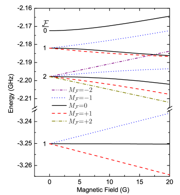
Figure 1 shows the Zeeman splitting of the hyperfine levels for the lowest two rotational levels of ⁸⁷Rb⁸⁸Sr at magnetic fields up to 20 G. The hyperfine coupling constant $b_{\rm F,Rb}$ is 2.60 GHz, which is reduced by about 25% from its atomic value of 3.42 GHz. The resulting splitting is 5.2 GHz, which is considerably larger than the rotational spacing of 1.1 GHz, so levels correlating with $f=2$ are well off the top of Fig. 1. The rotationless $N=0$ state, with $f=1$ and $F=1$ , splits into 3 sublevels with projection $M_{F}$ , just like a free ⁸⁷Rb atom. By contrast, the $N=1$ state with $F=f=1$ is split into three zero-field levels with ${\cal F}=0$ , 1 and 2 by the spin-rotation coupling. When a magnetic field is applied, each of these splits initially into $2{\cal F}+1$ components labeled by the total projection $M_{\cal F}$ . However, states of the same $M_{\cal F}$ originating from different ${\cal F}$ levels mix as the field increases; at higher fields, $\cal F$ is no longer a good quantum number and the magnetic sublevels are better described by $M_{F}$ and $M_{N}$ . In this regime, from 30 to about 1000 G, $F=f$ remains nearly conserved. At even higher fields, levels of different $F$ will mix and eventually the best quantum numbers are $M_{S}=m_{s}$ , $M_{I}=m_{i}$ and $M_{N}$ .

The situation is more complicated when the closed-shell atom has non-zero nuclear spin. We consider briefly the example of ⁸⁷Rb⁸⁷Sr, which is topical because Feshbach resonances have recently been observed for this combination Barbé et al. (2017). The largest coupling is still between $S$ and $i_{\rm Rb}$ to form $f_{\rm Rb}=1$ and 2, but in this case $f_{\rm Rb}=1$ couples to $i_{\rm Sr}=9/2$ to form $F=7/2$ , 9/2 and 11/2. There are thus 3 zero-field states even for $N=0$ , spread over about 160 MHz by the coupling between $i_{\rm Sr}$ and $S$ . For $N=1$ , these are each split into 3 by the spin-rotation coupling: $F=7/2\rightarrow{\cal F}=5/2,7/2,9/2$ , $F=9/2\rightarrow{\cal F}=7/2,9/2,11/2$ , $F=11/2\rightarrow{\cal F}=9/2,11/2,13/2$ . In a magnetic field these split into a total of $(2f_{\rm Rb}+1)(2i_{\rm Sr}+1)(2N+1)=90$ sublevels. The different angular momenta decouple sequentially as the magnetic field increases: first $N$ , then $i_{\rm Sr}$ and finally $i_{\rm Rb}$ . For $N>0$ there are additional hyperfine couplings due to nuclear quadrupole interactions [ $(eQq)_{\rm Rb}$ and $(eQq)_{\rm Sr}$ ] and anisotropic electron-nuclear spin couplings ( $t_{\rm Rb}$ and $t_{\rm Sr}$ ); these shift the resulting levels by a few MHz, but do not produce additional splittings. The resulting Zeeman diagram is very complicated and is beyond the scope of this paper to explore in detail.

The situation is different again for CaF and SrF. Here the chemical interaction is strong enough that an atomic $f$ quantum number for fluorine is not useful. The coupling between the electron and nuclear spins is much smaller than the separation between molecular rotational levels, so the ordering of levels is different. For even-mass Ca or Sr isotopes with $i=0$ the primary coupling is between $S=1/2$ and $i_{\rm F}=1/2$ to form $F=0$ and 1. The resulting levels have been explored in previous work Childs et al. (1981a). For ⁴³Ca and ⁸⁷Sr, however, the primary coupling is between $S=1/2$ and $i_{\rm Ca}=7/2$ or $i_{\rm Sr}=9/2$ . For ⁸⁷SrF these couple to form levels with $f_{\rm Sr}=4$ and $5$ , separated by about 2.6 GHz. These levels are then further split by weaker coupling to $i_{\rm F}=1/2$ to form zero-field $N=0$ states $F=7/2$ , 9/2, 9/2 and 11/2. For $N>0$ these are further split by spin-rotation coupling. ⁴³CaF behaves analogously.

It is noteworthy that both the isotropic and dipolar magnetic hyperfine couplings are a factor of 7 to 10 stronger for ¹⁷¹Yb in RbYb than for ⁸⁷Sr in RbSr. This makes ¹⁷¹Yb a particularly appealing candidate for Feshbach resonances such as those predicted in ref. Brue and Hutson (2012) and observed for ⁸⁷Rb⁸⁷Sr in ref. Barbé et al. (2017).

IV Conclusions

Hyperfine coupling in ${}^{2}\Sigma$ molecules containing alkaline-earth atoms is important both in producing ultracold molecules and in using them for applications in quantum science. We have used density-functional theory to calculate hyperfine coupling constants for several ${}^{2}\Sigma$ molecules that are the targets of current experiments aimed at producing ultracold molecules. We have focused on molecules formed from an alkaline-earth (or Yb) atom and either an alkali-metal atom or fluorine. The resulting hyperfine splitting patterns and Zeeman splittings are illustrated by considering isotopologs of RbSr and SrF.

Refer to caption — Figure 1: Zeeman splitting of the lowest hyperfine energy levels of ${}^{87}{\rm Rb}^{88}{\rm Sr}$ for magnetic fields up to 20 G.

Table 2: Coupling constants for the isotopologs of RbSr, LiYb, RbYb, CaF and SrF.

AX	$I_{\rm{A}}$	$I_{\rm{X}}$	$\gamma$ /MHz	$b_{\rm{F,A}}$ (MHz)	$t_{\rm{A}}$ (MHz)	$b_{\rm{F,X}}$ (MHz)	$t_{\rm{X}}$ (MHz)	$(eQq)_{\rm{A}}$ /MHz	$(eQq)_{\rm{X}}$ /MHz
⁸⁵Rb⁸⁴Sr	5/2	0	33.8	767	0.01	—	—	$-$ 7.5	—
⁸⁵Rb⁸⁶Sr	5/2	0	33.4	767	0.01	—	—	$-$ 7.5	—
⁸⁵Rb⁸⁷Sr	5/2	9/2	33.2	767	0.01	$-$ 65.2	$-$ 3.7	$-$ 7.5	$-$ 23.1
⁸⁵Rb⁸⁸Sr	5/2	0	33.0	767	0.01	—	—	$-$ 7.5	—
⁸⁷Rb⁸⁴Sr	3/2	0	33.4	2600	0.04	—	—	$-$ 3.6	—
⁸⁷Rb⁸⁶Sr	3/2	0	33.0	2600	0.04	—	—	$-$ 3.6	—
⁸⁷Rb⁸⁷Sr	3/2	9/2	32.8	2600	0.04	$-$ 65.2	$-$ 3.7	$-$ 3.6	$-$ 23.1
⁸⁷Rb⁸⁸Sr	3/2	0	32.6	2600	0.04	—	—	$-$ 3.6	—
⁶Li¹⁶⁸Yb	1	0	1880	97.2	0.1	—	—	$\approx$ 0	—
⁶Li¹⁷⁰Yb	1	0	1880	97.2	0.1	—	—	$\approx$ 0	—
⁶Li¹⁷¹Yb	1	1/2	1880	97.2	0.1	1440	83.1	$\approx$ 0	—
⁶Li¹⁷²Yb	1	0	1880	97.2	0.1	—	—	$\approx$ 0	—
⁶Li¹⁷³Yb	1	5/2	1880	97.2	0.1	$-$ 396	$-$ 22.9	$\approx$ 0	$-$ 786
⁶Li¹⁷⁴Yb	1	0	1880	97.2	0.1	—	—	$\approx$ 0	—
⁶Li¹⁷⁶Yb	1	0	1880	97.2	0.1	—	—	$\approx$ 0	—
⁷Li¹⁶⁸Yb	3/2	0	1620	257	0.2	—	—	0.1	—
⁷Li¹⁷⁰Yb	3/2	0	1620	257	0.2	—	—	0.1	—
⁷Li¹⁷¹Yb	3/2	1/2	1620	257	0.2	1440	83.1	0.1	—
⁷Li¹⁷²Yb	3/2	0	1620	257	0.2	—	—	0.1	—
⁷Li¹⁷³Yb	3/2	5/2	1620	257	0.2	$-$ 396	$-$ 22.9	0.1	$-$ 786
⁷Li¹⁷⁴Yb	3/2	0	1620	257	0.2	—	—	0.1	—
⁷Li¹⁷⁶Yb	3/2	0	1620	257	0.2	—	—	0.1	—
⁸⁵Rb¹⁶⁸Yb	5/2	0	54.9	844	0.02	—	—	$-$ 5.1	—
⁸⁵Rb¹⁷⁰Yb	5/2	0	54.7	844	0.02	—	—	$-$ 5.1	—
⁸⁵Rb¹⁷¹Yb	5/2	1/2	54.6	844	0.02	499	36.8	$-$ 5.1	—
⁸⁵Rb¹⁷²Yb	5/2	0	54.5	844	0.02	—	—	$-$ 5.1	—
⁸⁵Rb¹⁷³Yb	5/2	5/2	54.4	844	0.02	$-$ 137	$-$ 10.1	$-$ 5.1	$-$ 303
⁸⁵Rb¹⁷⁴Yb	5/2	0	54.3	844	0.02	—	—	$-$ 5.1	—
⁸⁵Rb¹⁷⁶Yb	5/2	0	54.1	844	0.02	—	—	$-$ 5.1	—
⁸⁷Rb¹⁶⁸Yb	3/2	0	54.1	2860	0.1	—	—	$-$ 2.3	—
⁸⁷Rb¹⁷⁰Yb	3/2	0	53.9	2860	0.1	—	—	$-$ 2.3	—
⁸⁷Rb¹⁷¹Yb	3/2	1/2	53.7	2860	0.1	499	36.8	$-$ 2.3	—
⁸⁷Rb¹⁷²Yb	3/2	0	53.6	2860	0.1	—	—	$-$ 2.3	—
⁸⁷Rb¹⁷³Yb	3/2	5/2	53.5	2860	0.1	$-$ 137	$-$ 10.1	$-$ 2.3	$-$ 303
⁸⁷Rb¹⁷⁴Yb	3/2	0	53.4	2860	0.1	—	—	$-$ 2.3	—
⁸⁷Rb¹⁷⁶Yb	3/2	0	53.2	2860	0.1	—	—	$-$ 2.3	—
⁴⁰Ca¹⁹F	0	1/2	37.2	—	—	127	8.0	—	—
⁴²Ca¹⁹F	0	1/2	36.6	—	—	127	8.0	—	—
⁴³Ca¹⁹F	7/2	1/2	36.3	$-$ 404	$-$ 3.0	127	8.0	9.9	—
⁴⁴Ca¹⁹F	0	1/2	36.1	—	—	127	8.0	—	—
⁴⁶Ca¹⁹F	0	1/2	35.6	—	—	127	8.0	—	—
⁴⁸Ca¹⁹F	0	1/2	35.2	—	—	127	8.0	—	—
⁸⁴Sr¹⁹F	0	1/2	70.5	—	—	112	6.8	—	—
⁸⁶Sr¹⁹F	0	1/2	70.2	—	—	112	6.8	—	—
⁸⁷Sr¹⁹F	9/2	1/2	70.1	$-$ 525	$-$ 3.8	112	6.8	$-$ 150	—
⁸⁸Sr¹⁹F	0	1/2	69.9	—	—	112	6.8	—	—

Table 3: Coupling constants for one isotopolog of RbSr, LiYb, RbYb, CaF and SrF calculated using restricted and unrestricted calculations.

AX	$I_{\rm{A}}$	Source	$I_{\rm{X}}$	$\gamma$ /MHz	$b_{\rm{F,A}}$ (MHz)	$t_{\rm{A}}$ (MHz)	$b_{\rm{F,X}}$ (MHz)	$t_{\rm{X}}$ (MHz)	$(eQq)_{\rm{A}}$ /MHz	$(eQq)_{\rm{X}}$ /MHz
⁸⁵Rb⁸⁷Sr	B3LYP-R	5/2	9/2	33.2	767	0.01	$-$ 65.2	$-$ 3.7	$-$ 7.5	$-$ 23.1
	B3LYP-U	5/2	9/2	26.7	893	$-$ 0.50	$-$ 52.1	$-$ 3.8	$-$ 7.3	$-$ 23.3
⁷Li¹⁷³Yb	B3LYP-R	3/2	5/2	1620	257	0.2	$-$ 396	$-$ 22.9	0.1	$-$ 786
	B3LYP-U	3/2	5/2	1190	364	0.2	$-$ 294	$-$ 20.5	0.1	$-$ 673
⁸⁵Rb¹⁷³Yb	B3LYP-R	5/2	5/2	54.4	844	0.02	$-$ 137	$-$ 10.1	$-$ 5.1	$-$ 303
	B3LYP-U	5/2	5/2	40.9	962	$-$ 0.16	$-$ 105	$-$ 9.0	$-$ 4.8	$-$ 257
⁴³Ca¹⁹F	B3LYP-R	7/2	1/2	36.3	$-$ 404	$-$ 3.0	127	8.0	9.9	—
	B3LYP-U	7/2	1/2	38.9	$-$ 443	$-$ 4.8	126	8.2	10.2	—
⁸⁷Sr¹⁹F	B3LYP-R	9/2	1/2	70.1	$-$ 525	$-$ 3.8	112	6.8	$-$ 150	—
	B3LYP-U	9/2	1/2	65.2	$-$ 570	$-$ 6.0	114	7.0	$-$ 154	—

Appendix A Supplemental Material

Table LABEL:table:table4 gives results for both spin-restricted and spin-unrestricted DFT calculations using the B3LYP Stephens et al. (1994) and PBE0 Perdew et al. (1996) functionals, for a variety of ${}^{2}\Sigma$ molecules for which experimental values are available. Overall, B3LYP is a little more accurate than PBEO and so we use B3LYP in the main paper. The largest fractional discrepancies are mostly in cases where the constants concerned are small, and thus play a minor role for the molecule in question. In these cases the calculations correctly give small values, though sometimes with substantial percentage errors. For the remaining molecules, the spin-restricted results for $\Delta g_{\bot}$ (or equivalently $\gamma$ ) are accurate to 30% or better, with the exceptions of GaO and InO. The agreement is significantly better for $b_{\rm{F}}$ and $t$ , except for InO. The exceptions probably arise because the ground states of these oxide radicals are mixtures of two electronic configurations with similar energies Knight et al. (1997). Molecular properties such as hyperfine coupling constants are very sensitive to the balance between the configurations.

Unrestricted calculations are often slightly more accurate than restricted calculations, especially for $\gamma$ . However, in some cases they give very poor results, even where the fine and hyperfine coupling constants are large: see, for example, the values of $b_{\rm{F}}$ for the metals in AlO, GaO and InO. It appears that unrestricted calculations on these oxides are even more susceptible to mixing of configurations than restricted calculations. The unrestricted B3LYP calculation also give dramatically incorrect results for $\gamma$ in LiBa: in this case we have calculated the effective spin of the molecule, and find that its value is far from 1/2 in the unrestricted case, so it is clear that the solution suffers from spin contamination.

We conclude that spin-restricted B3LYP calculations give the most reliable overall results. It is however valuable carry out unrestricted calculations as well: in cases where the two are similar, the unrestricted result may be better.

Table 4: Comparison between experimental and theoretical values of

\Delta g_{\bot}

\gamma

b_{\rm F}

and

t

for

{}^{2}\Sigma

molecules computed through restricted (R) and unrestricted (U) DFT calculations using the B3LYP Stephens et al. (1994) and PBE0 Perdew et al. (1996) functionals. An asterisk indicates cases where the signs of the components of the

{\bm{A}}

tensor were not reported in the experimental papers and have been assigned to match the theoretical results Verma and Autschbach (2013). The acronyms GP, NM and AM stand for “Gas Phase”, “Neon Matrix” and “Argon Matrix” respectively and refer to the conditions used to record the spectra. Experimental results labelled as “CA” are obtained by applying Curl’s approximation to

\Delta g_{\bot}

\gamma