Coplanar Repeats by Energy Minimization

Abstract

This paper proposes an automated method to detect, group and rectify arbitrarily-arranged coplanar repeated elements via energy minimization. The proposed energy functional combines several features that model how planes with coplanar repeats are projected into images and captures global interactions between different coplanar repeat groups and scene planes. An inference framework based on a recent variant of $\alpha$-expansion is described and fast convergence is demonstrated. We compare the proposed method to two widely-used geometric multi-model fitting methods using a new dataset of annotated images containing multiple scene planes with coplanar repeats in varied arrangements. The evaluation shows a significant improvement in the accuracy of rectifications computed from coplanar repeats detected with the proposed method versus those detected with the baseline methods.

1 Introduction

The importance of detecting and modeling imaged repeated scene elements grows with the increasing usage of scene-understanding systems in urban settings, where man-made objects predominate and coplanar repeated structures are common. Most state-of-the-art repeat detection and modeling methods take a greedy approach that follows appearance-based clustering of extracted keypoints with geometric verification. Greedy methods have a common drawback: Sooner or later the wrong choice will be made in a sequence of threshold tests resulting in an irrevocable error, which makes a pipeline approach too fragile for use on large image databases.

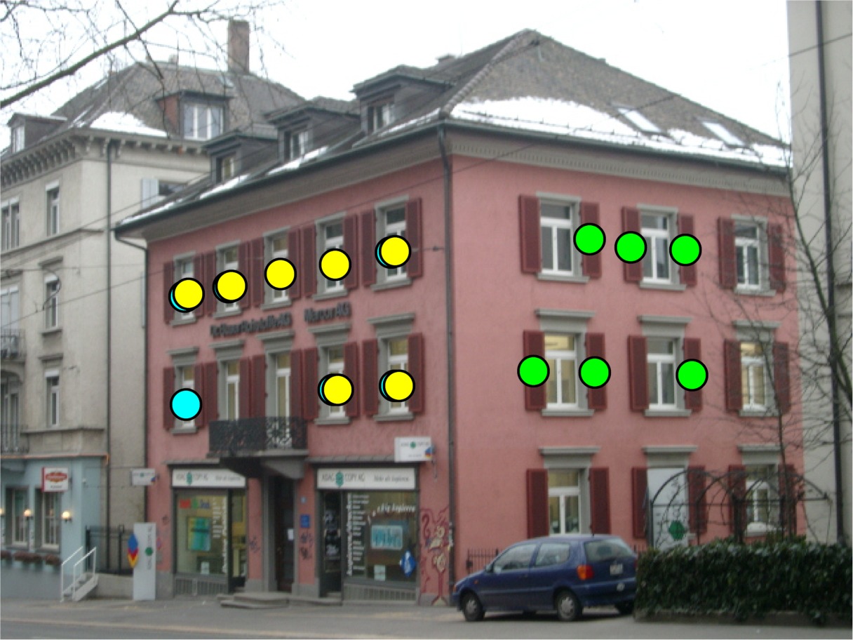
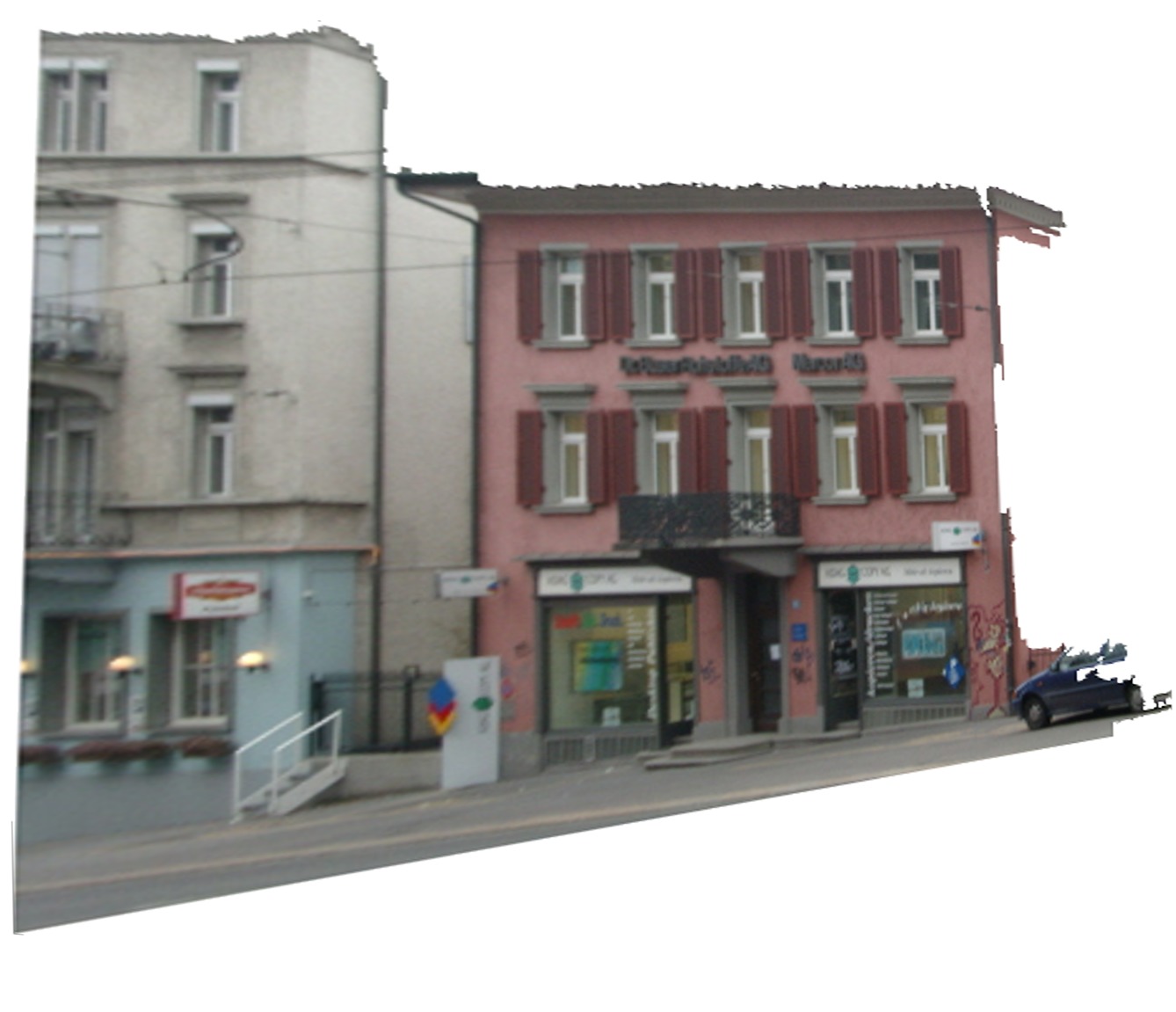
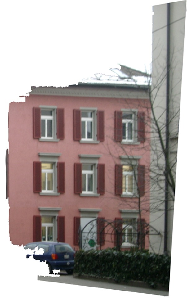
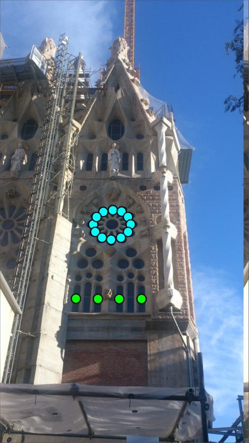
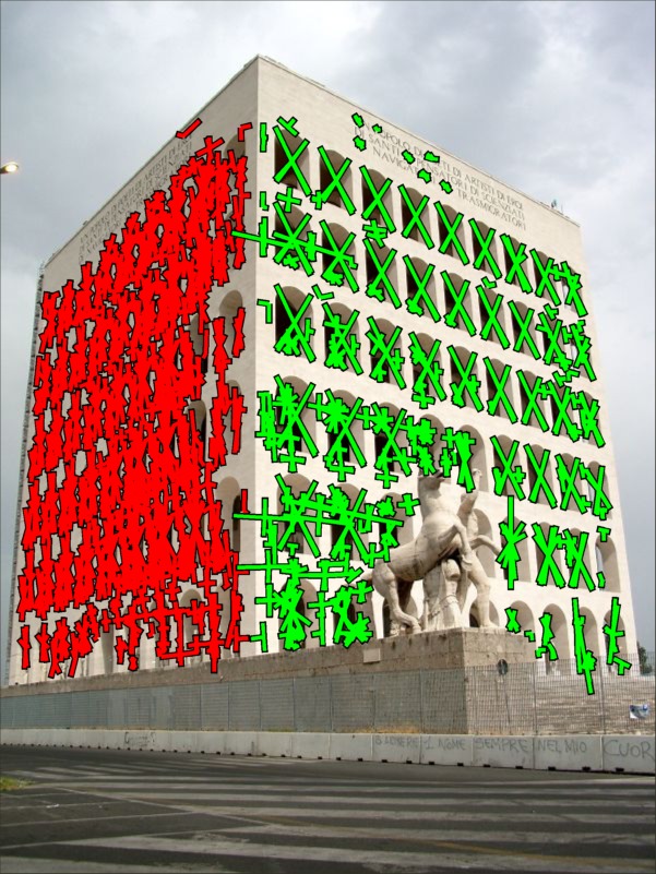
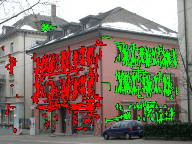
We propose a global energy model for grouping coplanar repeats and scene plane detection. The energy functional combines features encouraging (i) the geometric and appearance consistency of coplanar repeated elements, (ii) the spatial and color cohesion of detected scene planes, (iii) and a parsimonious model description of coplanar repeat groups and scene planes. The energy is minimzed by block-coordinate descent, which alternates between grouping extracted keypoints into coplanar repeats by labeling (see Figs. 1,2) and regresses the continuous parameters that model the geometries and appearances of coplanar repeat groups and their underlying scene planes. Inference is fast even for larger problems (see section 6).

Comparison to state-of-the-art coplanar repeat detection methods is complicated by the fact that many prior methods were either evaluated on small datasets, include only qualitative results, or were restricted to images with repeats having a particular symmetry. We evaluate the proposed method on a new annotated dataset of 113 images. The images have from 1 to 5 scene planes containing translation, reflection, or rotation symmetries that repeat periodically or arbitrarily. Performance is measured by comparing the quality of rectifications computed from detected coplanar repeat groups versus rectifications computed from the annotated coplanar repeat groups of the dataset.

(a)	(b)	(c)	(d)	(e)

Figure 1: Grouping and rectification of coplanar repeats: (a) a subset of the detected coplanar repeats is denoted by colored dots, (b) rectification of the most distant keypoint pairs grouped as coplanar repeats—repeat group membership is encoded by the colored border, (c,d) rectified and segmented scene planes, (e) Translation and rotation symmetric keypoints labeled as distinct coplanar repeats.

2 Related Work

Repeat grouping is a well-studied computer vision task. Many variants of hypothesize-and-verify pipelines were proposed in the prior literature for grouping repeats. Typical distinctions between methods are the variants of used feature types, geometric constraints, and scene geometry estimators. Two closely related early methods by Schaffalitzky et al [Schaffalitzky and Zisserman(1998)] and Tuytelaars et al [Tuytelaars et al.(2003)Tuytelaars, Turina, and Van Gool] estimate homologies that are compatible with detected fixed points and lines induced by periodicities, symmetries and reflections of scene elements. Liebowitz et al [Liebowitz and Zisserman(1998)] use metric invariants to identify repeats in an affine-rectified frame estimated from imaged parallel scene lines.

More recent approaches eliminate the need for any scene structure other than the coplanar repeated scene elements and work for arbitrarily arranged repeats (i.e., rigidly transformed on the scene plane). Chum et al [Chum and Matas(2010)] introduce an algebraic constraint on the local scale change of a planar feature and use it to verify that tentative repeats have equal scale in a rectified frame (this constraint is included in the proposed energy function). Pritts et al [Pritts et al.(2014)Pritts, Chum, and Matas] introduce constraints specific to rotated and reflected repeated elements in an affine rectified frame and generatively build a model of the pattern rectified to within a similarity of the scene.

Two frequently cited approaches use energy minimization frameworks. Park et al [Park et al.(2009)Park, Brocklehurst, Collins, and Liu] minimize an energy that measures the compatibility of a deformable lattice to imaged uniform grids of repetitions. Wu et al [Wu et al.(2010)Wu, Frahm, and Pollefeys] refine vanishing point estimates of an imaged building facade by minimizing the difference between detected symmetries across repetition boundaries of the facade.

None of the reviewed approaches globally model repeats; rather, there is an assumption that a dominant plane is present, or repeat grouping proceeds greedily by detecting scene planes sequentially. A significant subset of the reviewed literature requires the presence of special scene structure like parallel scene lines or lattices, which limits their applicability.

3 Scene Model

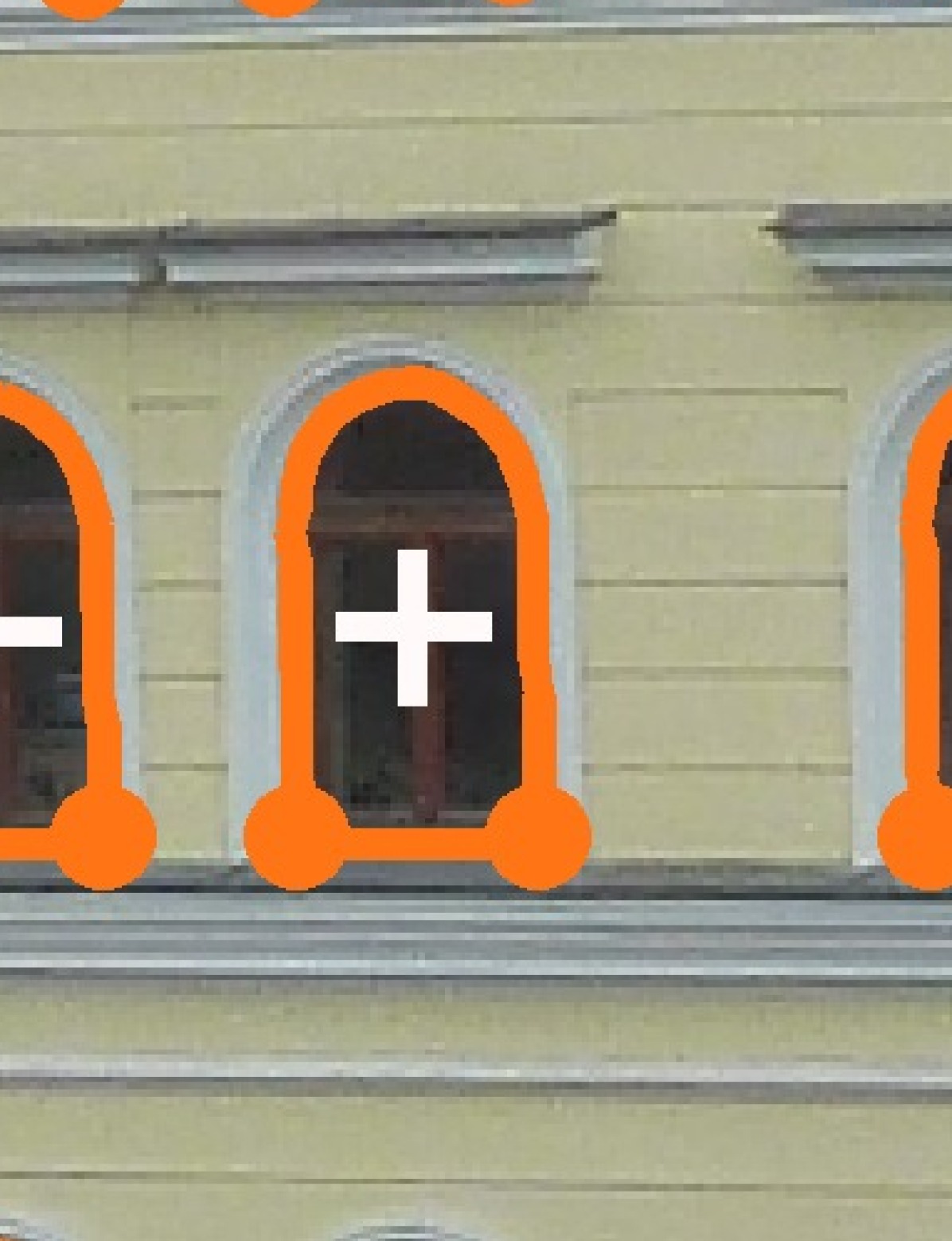
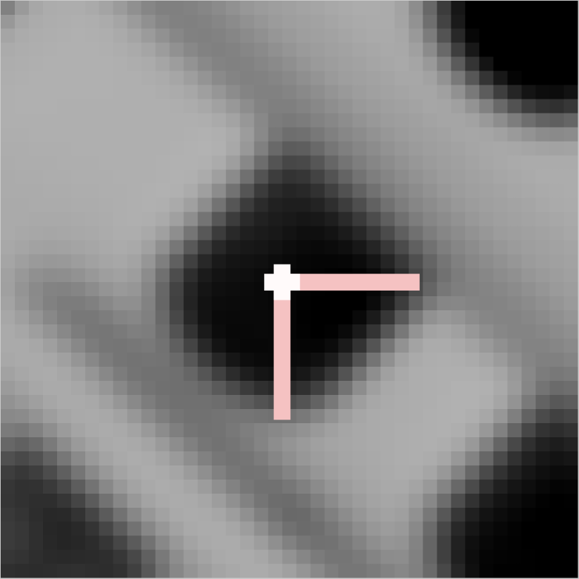
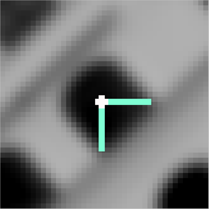
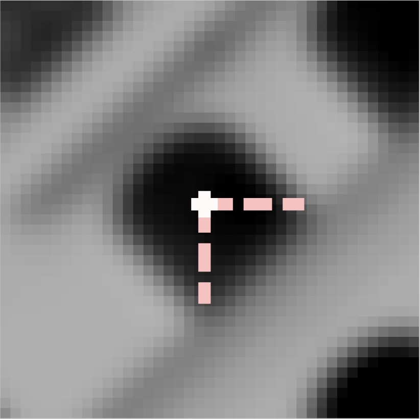
The scene model has three types of outputs: The first output is a grouping of detected keypoints (see Figs. 2a-2d) into coplanar repeats (see Figs. 1a,1e). Random variables $Y^{K}$ jointly assign keypoints to keypoint groups with mutually compatible geometry and appearance and to planar scene surfaces. Each random variable of $Y^{K}$ is from the set $\mathcal{Y}_{K}=\{\,1\ldots N_{G},\,\varnothing\,\}\times\{\,1\dots N_{V},b\,\}$. Here $N_{G}$ is the number of clusters of keypoints that were grouped based on their similarity in appearance, and $N_{V}$ is the estimated number of planar surfaces in the scene. A particular labeling of $Y^{K}$ is denoted $\mathbf{y}^{K}$. The assignment of the $i$-th keypoint to a compatible keypoint cluster is indexed as $\mathbf{y}^{K}_{ig}$, and its assignment to a scene plane is indexed as $\mathbf{y}^{K}_{iv}$. The empty set $\varnothing$ is assigned if keypoint $i$ does not repeat, $\mathbf{y}^{K}_{ig}=\varnothing$, and the token $b$ is assigned to a keypoint if it does not lie on a planar surface. Background keypoints cannot be assigned to a repeat group, so they are assigned the ordered pair $(\,\varnothing,b\,).$ The non-planar surfaces are collectively called the background. The sets of keypoints assigned to the same keypoint cluster and scene plane are the coplanar repeated patterns.

Term	Description	Term	Description
$\mathbf{x}^{K}_{i}$	keypoint, see Fig. 2d	$\varnothing$	keypoint is a singelton
$\mathbf{x}^{K}_{iw}$	point of a keypoint	$N_{G}$	number of keypoint clusters
$\mathbf{x}^{R}_{j}$	image region, see Fig. 2e	$N_{V}$	number of scene planes
$\mathbf{x}$	all measurements	$\beta^{K}(\mathbf{y}^{K})$	geom./app. params. for repeats
$\mathbf{y}^{K}_{ig}$	keypoint $\leftrightarrow$ cluster	$\beta^{R}(\mathbf{y}^{K},\mathbf{y}^{R})$	geom./app. params. for planes
$\mathbf{y}^{K}_{iv}$	keypoint $\leftrightarrow$ scene plane	$\beta(\mathbf{y})$	joint parameter vector
$\mathbf{y}^{K}_{i}$	keypt. label, $(\mathbf{y}^{K}_{ig},\mathbf{y}^{K}_{iv})$, see Fig. 1a	$\psi(\cdot)$	joint feature vector
$\mathbf{y}^{R}_{j}$	region $\leftrightarrow$ scene plane, see Fig. 1d	$\mathbf{w}$	feature weight vector
$\mathbf{y}$	joint labeling	$\mathbf{l}_{n}$	scene plane vanishing line
b	keypt./region is on background	$H_{\mathbf{l}_{n}}(\cdot)$	rectifying transform from $\mathbf{l}_{n}$

Table 1: The most commonly used scene model denotations.

The second output is a labeling of image regions as planar surfaces and background. The image regions are small and connected areas of similar color that are detected as SEEDS superpixels [Van den Bergh et al.(2012)Van den Bergh, Boix, Roig, de Capitani, and Van Gool] (see Fig. 2e). Random variables $Y^{R}$ assign image regions to planar surfaces and the background, where each random variable of $Y^{R}$ is from the set $\mathcal{Y}_{R}=\{\,1\dots N_{V},b\,\}$. As before, $N_{v}$ and $b$ are the estimated number of planar surfaces and the background token, respectively. A particular labeling of $Y^{R}$ is denoted $\mathbf{y}^{R}$, and the labeling partitions the image regions into larger components that correspond to contiguous planar surfaces of the scene or background. The assignment of the $j$-th region to a scene plane or to background is indexed as $\mathbf{y}^{R}_{j}$.

The third output is a set of continuous random variables modeling the geometries and appearances of the sets of coplanar repeats and the scene planes. The geometries and appearances of coplanar repeats are functions of the keypoint assignments and are given by the dependent random variables $B^{K}(Y^{K})$. The corresponding parameter estimates are denoted as $\beta^{K}(\mathbf{y}^{K})$. The geometries and appearances of the scene planes are functions of $Y^{K}$ and $Y^{R}$, and are given by dependent random variables $B^{R}(Y^{K},Y^{R})$. The parameters $\beta^{R}(\mathbf{y}^{K},\mathbf{y}^{R})$ represent the colors of the scene surfaces and the orientations of scene planes.

The joint labeling and parameter vector for the entire model are respectively denoted $\mathbf{y}={\mathbf{y}^{K}}^{\frown}{\mathbf{y}^{R}}$ and $\beta(\mathbf{y})={\beta^{K}}(\mathbf{y}^{K})^{\frown}\beta^{R}(\mathbf{y}^{K},\mathbf{y}^{R})$.

3.1 Energy Function

The joint feature vector $\psi(\cdot)$ encodes potentials that measure (i) coplanar repeats consist of keypoints that have similar appearnace and the same area in the preimage, (ii) the scene planes and background should consist of image regions with the same color distributions, (iii) surfaces should be contiguous and that nearby repeated content should be on the same surface, (iv) and scenes should have a parsimonious description. A minimal energy labeling $\mathbf{y}$ and parameter set $\beta(\mathbf{y})$ are sought by solving the energy minimization task

$$\operatorname*{argmin}_{\mathbf{y},\beta}\,\underbrace{\mathbf{w}^{{\!\top}}\psi(\mathbf{x},\mathbf{y},\beta(\mathbf{y}))}_{E\text{ (energy)}},$$ (1)

where $\mathbf{x}$ are the detected salient image patches and over-segmented regions of the image, and $\mathbf{w}$ is a weight vector. The components of $\mathbf{w}$ take on different meanings depending on their paired features and are discussed in Sections 3.3 to 3.5.

(a)	(b)	(c)	(d)	(e)	(f)

Figure 2: Image measurements. (a) Center of gravity (white cross) and curvature extrema (orange circles) of a detected MSER (orange contour [Matas et al.(2002a)Matas, Chum, Urban, and Pajdla]). (b) Patches are normalized and oriented to define an affine keypoint as in [Matas et al.(2002b)Matas, Obdržálek, and Chum], and their texture is described by RootSIFT [Arandjelović and Zisserman(2012), Lowe(2004)] (c) Bases are reflected for symmetry detection. (d) Affine keypoints mapped back into image. (e) Over-segmentation by superpixels. (f) The contrast feature $\psi^{\text{contrast}}_{T}$, where intensity is proportional to edge response along superpixel boundaries.

3.2 Measurements

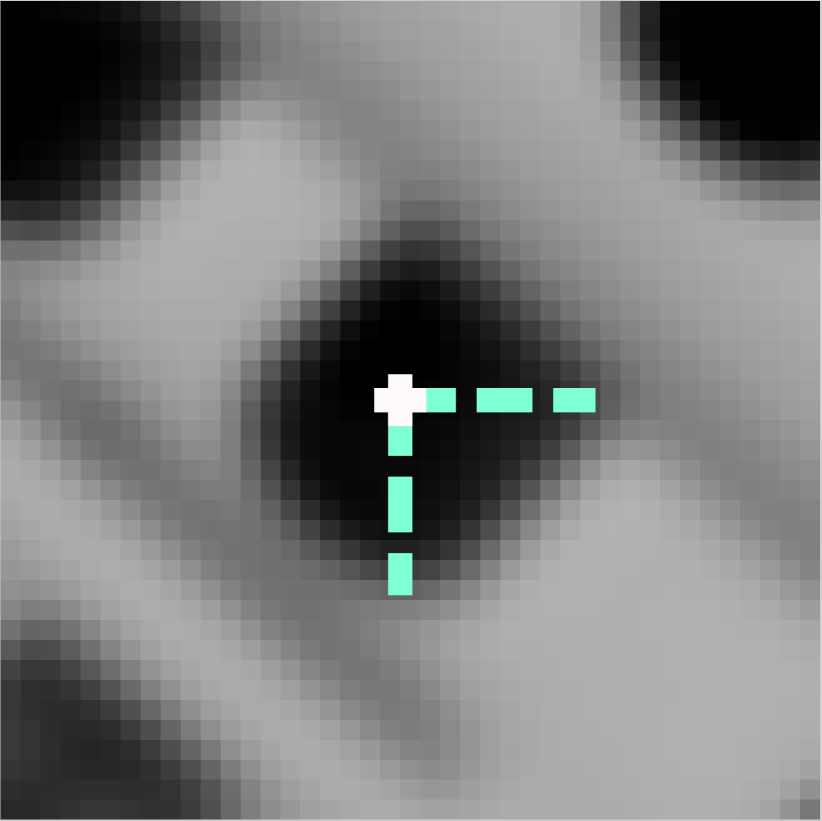
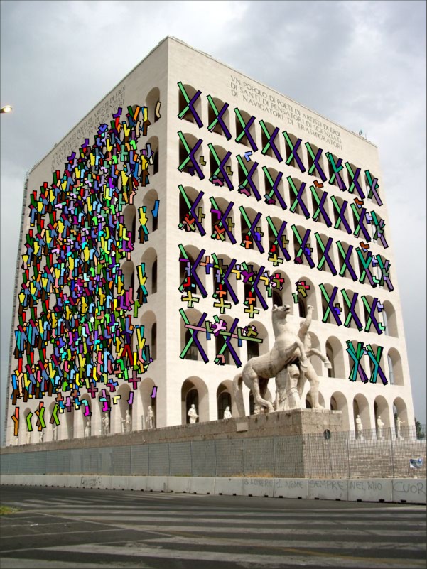
Affine-covariant keypoints [Matas et al.(2002a)Matas, Chum, Urban, and Pajdla, Mikolajczyk and Schmid(2004), Obdržálek and Matas(2002)] are extracted from the image as good candidates for representing repeated content. (see Fig. 2a). The shapes of the detected patches are summarized by keypoints, or, equivalently, 3-tuples of points, and are given by measurements $\mathbf{x}^{K}$. One type of keypoint construction is illustrated in Figs. 2a-d. The image is over-segmented by SEEDS superpixels [Van den Bergh et al.(2012)Van den Bergh, Boix, Roig, de Capitani, and Van Gool] to provide measurements on regions where keypoint detection is unlikely (see Fig. 2e). The segmented regions are denoted by $\mathbf{x}^{R}$. The keypoints and regions are concatenated to give the joint measurement $\mathbf{x}={\mathbf{x}^{K}}^{\frown}\mathbf{x}^{R}$, which is an argument to the energy defined in Eq. 1.

3.3 Unary Features for Repeats and Surfaces

The perspective skew of each scene plane is given by its vanishing line, which is an analog to the horizon line for a scene plane at any orientation. Vanishing lines are encoded in the parameters of the scene planes $\beta^{R}(\mathbf{y}^{K},\mathbf{y}^{R})$. Explicitly they are the set $\{\,\mathbf{l}_{n}\,\mid\,\mathbf{l}_{n}\in\mathcal{P}^{2}\,\}_{n=1}^{N_{V}}$, where $N_{V}$ is the number of scene planes and $\mathcal{P}^{2}$ is the real projective plane.

Scale of coplanar repeats.

A coplanar repeat group $C$ is the set of keypoints from the same pattern that co-occur on a scene plane, namely $C=\{\,\mathbf{x}^{K}_{i}\,\mid\,\mathbf{y}^{K}_{ig}=m\,\wedge\,\mathbf{y}^{K}_{iv}=n\,\}$, where $n\neq b$. The keypoints of $C$ are called coplanar repeats. The coplanar repeats of $C$ are of equal scale (equiareal) if their perspective skew is removed, which is accomplished by transforming the vanishing line of the underlying scene plane $\mathbf{l}_{n}$ so that it is coincident with the principal axis of the camera (see Chum et al[Chum and Matas(2010)]). The scale feature $\psi^{\text{scale}}$ measures the mutual compatibility of coplanar repeats with the scale constraint. Let $H_{\mathbf{l}_{n}}(\cdot)$ be a transformation that removes perspective skew from plane $n$ by orienting $\mathbf{l}_{n}$ to the principal axis and $s(\cdot)$ be the function that computes the scale of a keypoint. Then the scale feature for the scene’s coplanar repeats is

$$\psi^{\text{scale}}=-\sum_{m=1}^{N_{G}}\,\sum_{n=1}^{N_{V}}\,\sum_{i}\,[\mathbf{y}^{K}_{ig}=m]\cdot[\mathbf{y}^{K}_{iv}=n]\cdot\left(\log s(H_{\mathbf{l}_{n}}(\mathbf{x}^{K}_{i}))-\log\,\bar{s}(n,\mathbf{y}^{K}_{ig})\right)^{2},$$ (2)

where $\bar{s}(n,\mathbf{y}^{K}_{ig})$ is the geometric mean of the keypoints in pattern $\mathbf{y}^{K}_{ig}$ rectified by transformation $H_{\mathbf{l}_{n}}(\cdot)$, which is part of the estimated parameters of the repeated scene content encoded in $\beta^{F}(\mathbf{y}^{K})$.

Appearance of patterns.

The appearance of the image patches containing the keypoints $\mathbf{x}^{K}$ are described by RootSIFT [Arandjelović and Zisserman(2012), Lowe(2004)]. The corresponding RootSIFT of a keypoint is given by the function $u(\cdot)$. The appearance affinity of keypoint $\mathbf{x}^{K}_{i}$ to a pattern is given by the normalized Euclidean distance between the RootSIFT descriptor of the keypoint and mean RootSIFT descriptor of the pattern. The appearance feature for patterns is

$${\psi}^{\text{app}}=\sum_{m=1}^{N_{G}}\,\sum_{i}\,[\mathbf{y}^{K}_{ig}=m]\cdot\frac{\|u(\mathbf{x}^{K}_{i})-\bar{u}(\mathbf{y}^{K}_{ig})\|_{2}^{2}}{\sigma_{1}^{2}},\\$$ (3)

where $\bar{u}(\mathbf{y}^{K}_{ig})$ is the mean of the RootSIFTs of keypoints in pattern $\mathbf{y}^{K}_{ig}$, which is part of the estimated parameters of the repeated scene content encoded in $\beta^{F}(\mathbf{y}^{K})$. The variance $\sigma_{1}^{2}$ is set empirically.

Color of scene surfaces.

The color distribution of each scene surface is modeled with a RGB Gaussian mixture model (GMM) with $K$ components, $\gamma=\{\,\mu_{nk},\Sigma_{nk},\pi_{nk},\}$, where $nk\in\{\,1\dots N_{V},\,b\,\}\times\{\,1\ldots K\,\}$ and $\mu_{nk},\Sigma_{nk},\pi_{nk}$ are the mean RGB color, full color covariance and mixing weight for component $k$ of surface $v$. The set of GMM parameters $\gamma$ is part of the estimated parameters of the appearance and geometry for scene planes encoded in $B^{R}(Y^{K},Y^{R})$. The color feature for the scene surfaces is

$$\psi^{\text{color}}=\sum_{n\in\{1\ldots N_{V},b\}}\,\sum_{j}\,\sum_{j^{\prime}}\,\frac{[\mathbf{y}^{R}_{jv}=n]}{|\mathbf{x}^{R}_{j}|}\cdot\underbrace{\min_{k\in\{1,\ldots,K\}}\left\{\,-\log\left(p_{n}(\mathbf{x}^{R}_{jj^{\prime}}|k)\cdot\pi_{nk}\right)\,\right\}}_{\text{approximately $\propto-\log p_{n}(\mathbf{x}^{R}_{jj^{\prime}})$}},$$ (4)

where $\mathbf{x}^{R}_{jj^{\prime}}$ is the $j^{\prime}$-th member pixel of region $\mathbf{x}^{R}_{j}$ with $|\mathbf{x}^{R}_{j}|$ number of pixels and the conditional likelihood of a pixel $\mathbf{x}^{R}_{jj^{\prime}}$ given a mixture component $k$ is normally distributed, $\mathbf{x}^{R}_{jj^{\prime}}|k\sim\mathcal{N}(\mu_{nk},\Sigma_{nk})$. The feature $\psi^{\text{color}}$ uses the same approximation for the log-likelihood as Grabcut [Rother et al.(2004)Rother, Kolmogorov, and Blake] to make the maximum-likelihood estimation of GMM parameters faster. Connected components of regions with the same surface assignment segment the image into contiguous planar and background regions.

Planar and background singletons.

Singletons are keypoints that don’t repeat. A weighted cost for each singleton is assessed, which is the maximum unary energy that can be considered typical for a coplanar repeat. For a complete geometric parsing of the scene, it is necessary to assign each singleton to its underlying scene plane or to the background surface. Singletons induce no single-view geometric constraints nor appearance constraints because they are not part of a repeat group, so their assignments to scene planes are based on their interactions with neighborhood keypoints and regions, which are defined in section 3.4 as assignment regularization functions. An additional weighted cost for each planar singleton is assessed, which is the minimum amount of required evidence obtained through interactions with neighboring keypoints and regions to consider a singleton planar.

3.4 Pairwise

The pairwise features are a set of bivariate Potts functions that serve as regularizers for keypoint and region assignment to scene model components.

Keypoint contrast.

The keypoint contrast feature penalizes models that over-segment similar looking repeats. The keypoint contrast of the scene is

$$\psi^{\text{contrast}}_{F}=\sum_{i\neq i^{\prime}}[\mathbf{y}^{K}_{iv}\neq\mathbf{y}^{K}_{i^{\prime}v}]\cdot\exp\left[-\frac{\|u(\mathbf{x}^{K}_{i})-u(\mathbf{x}^{K}_{i^{\prime}})\|_{2}^{2}}{\sigma_{2}^{2}}\right],$$ (5)

where the variance $\sigma_{2}^{2}$ is set empirically.

Region contrast.

Regions have bounded area, so there may be large areas of low texture on a scene plane or in the background that are over-segmented. Regions that span low-texture areas can be identified by a low cumulative edge response along their boundary. The cumulative edge response between two regions, denoted $\phi(\mathbf{x}^{R}_{j},\mathbf{x}^{R}_{j^{\prime}})$, is robustly calculated so that short but extreme responses along the boundary do not dominate (see Fig. 2f). The region contrast of the image is given by the feature

$$\psi^{\text{contrast}}_{R}=\sum_{j\neq j^{\prime}}[\mathbf{y}^{R}_{jv}\neq\mathbf{y}^{R}_{j^{\prime}v}]\cdot\exp\left[-\frac{\phi(\mathbf{x}^{R}_{j},\mathbf{x}^{R}_{j^{\prime}})^{2}}{\lambda}\right].$$ (6)

A larger constant $\lambda$ increases the amount of smoothing and is set as $\lambda=2\cdot\bar{\phi^{2}}$, which puts the crossover point of smoothing at the mean contrast of regions.

Keypoint overlap.

A keypoint that overlaps a region is coplanar or co-occurs on the background surface with the overlapped region, which is encoded as a pairwise constraint. A penalty for each violation of the coplanarity constraint is assessed.

3.5 Label subset costs

Parsimonious scene models are encouraged by assessing a cost for each scene model part. Equivalence classes of the label set are defined by labels that share a scene model part, e.g, the set of labels that have the same vanishing line. A label subset cost is assessed if at least one label from an equivalence class is used, which is equivalent to accumulating a weighted count of the number of unique scene model components in the scene.

4 Energy Minimization

The energy minimization task of Eq. 1 is solved by alternating between finding the best labeling $\mathbf{y}$ and regressing the scene model components $\beta$ in a block-coordinate descent loop until the energy converges. Alternating between finding the minimal energy labeling and regressing continuous model parameters has notably been used in segmentation and multi-model geometry estimation by Rother et aland Isack et al[Rother et al.(2004)Rother, Kolmogorov, and Blake, Isack and Boykov(2012)].

4.1 Labeling and Regression

The scene model parameters are fixed to the current estimate for the labeling problem, $\hat{\mathbf{y}}=\operatorname*{argmin}_{\mathbf{y}}\,E(\mathbf{x},\mathbf{y},\beta(\mathbf{y})=\hat{\beta})$. Finding the minimal-energy labeling is NP-hard [Boykov et al.(2001)Boykov, Veksler, and Zabih]. An extension to alpha-expansion by Delong et al[Boykov et al.(2001)Boykov, Veksler, and Zabih, Delong et al.(2012)Delong, Osokin, Isack, and Boykov, Kolmogorov and Zabih(2004)] that accommodates label subset costs (defined in section 3.5) is used to find an approximate solution.

The labeling is fixed to the current estimate for the regression subtask $\hat{\beta}=\operatorname*{argmin}_{\beta}\,E(\mathbf{x},\mathbf{y}=\hat{\mathbf{y}},\beta(\hat{\mathbf{y}})).$ Each continuous parametric model must be regressed with respect to its dependent unary potentials so that the energy does not increase during a descent iteration. In particular, the vanishing lines, surface color distributions and the representative appearance for patterns and rectified scale for coplanar repeats are updated as detailed in the following paragraphs. The updated parameters are aggregated in $\hat{\beta}$.

Vanishing lines.

All keypoints assigned to the same planar surface are used to refine the surface’s vanishing line orientation. The objective is the same as the unary defined in eq. 2 and encodes the affine scale invariant defined in Chum et al[Chum and Matas(2010)]. The vanishing line is constrained to the unit sphere and so that all keypoints are on the same side of the oriented vanishing line,

$$\mathbf{l}^{*}_{n}=\operatorname*{argmin}_{\mathbf{l}}\sum_{i\,:\,\mathbf{\hat{y}}^{K}_{iv}=n}\left(\log s(H_{\mathbf{l}}(\mathbf{x}^{K}_{i}))-\frac{1}{\sum_{i^{\prime}}\,[\mathbf{\hat{y}}^{K}_{ig}=\mathbf{\hat{y}}^{K}_{i^{\prime}g}]}\log\sum_{i^{\prime}}\,[\mathbf{\hat{y}}^{K}_{ig}=\mathbf{\hat{y}}^{K}_{i^{\prime}g}]\cdot s(H_{\mathbf{l}}(\mathbf{x}^{K}_{i^{\prime}}))\right)^{2}$$ (7)

$$\begin{aligned} \textup{s.t.}\quad\mathbf{l}^{{\!\top}}\mathbf{x}^{K}_{iw}&>0,\quad w\in\{\,1\dots 3\,\}\\ \mathbf{l}^{{\!\top}}\mathbf{l}&=1,\\ \end{aligned}$$ (8)

for all scene planes $n$ that have patterns assigned, where $s(\cdot)$ is the scale of a keypoint and $H_{\mathbf{l}}(\cdot)$ is the rectifying transform as defined in section 3.3, and $\mathbf{x}^{K}_{iw}$ denotes the individual homogeneous coordinates that define keypoint $\mathbf{x}^{K}_{i}$. The constrained nonlinear program is solved with the MATLAB intrinsic fmincon.

Coplanar repeats and patterns.

For features $\psi^{\text{scale}}$ eq. (2) and $\psi^{\text{app}}$ eq. (3) that are sums of squared differences, the parameters are estimated as a mean of the respective values.

Surface color distribution.

The parameters of the color distribution of a surface are estimated from the member pixels of regions assigned to the surface. The approximate log-likelihood defined for the unary $\psi^{\text{color}}$ in eq. 4 is maximized to estimate the Gaussian mixture for each surface that has region assignments,

$$\{\,\Sigma^{*}_{nk},\mu^{*}_{nk},\pi^{*}_{nk}\,\}_{k=1}^{K}=\operatorname*{argmax}_{\{\Sigma_{nk},\mu_{nk},\pi_{nk}\}_{k=1}^{K}}\,\prod_{j:\mathbf{\hat{y}}^{R}_{j}=n}\,\prod_{j^{\prime}}\max_{k^{\prime}}\,p_{v}(\mathbf{x}^{R}_{jj^{\prime}}\mid k^{\prime};\Sigma_{nk},\mu_{nk},\pi_{nk})\cdot\pi_{nk^{\prime}}.$$ (9)

The objective defined in eq. 9 is maximized by block-coordinate ascent in a manner similar to Lloyd’s algorithm: The mixture component assignments are fixed to estimate the means and covariances and then vice-versa in alternating steps. A fixed number of iterations is performed.

4.2 Proposals

The initial minimal labeling energy requires a guess $\beta^{{0}}$ at the continuous parameters $\beta(\mathbf{y})$. This is provided by a proposal stage in which the keypoints $\mathbf{x}^{K}$ are clustered by their RootSIFT descriptors and sampled to generate vanishing line hypotheses as in Chum et al[Chum and Matas(2010)]. The clustered regions are verified against the hypothesized vanishing lines to create a putative collection of coplanar repeats that are scale-consistent after affine rectification by a compatible sampled vanishing line. The proposed coplanar repeat groups do not partition the keypoints, which is a constraint enforced by the minimal energy labeling $\mathbf{\hat{y}}$. The inital color model for each detected surface (equivalently proposed vanishing lines and background) is estimated from the image patches of keypoints from the proposed coplanar repeat groups.

5 Dataset

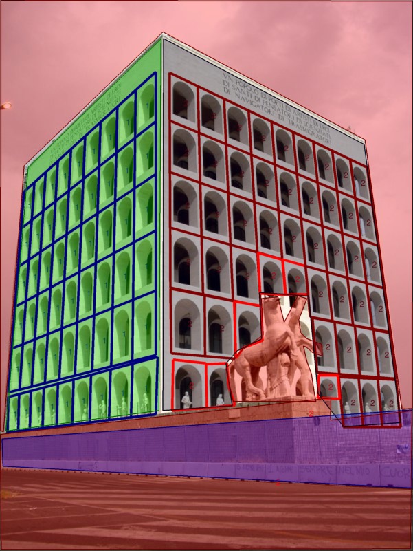
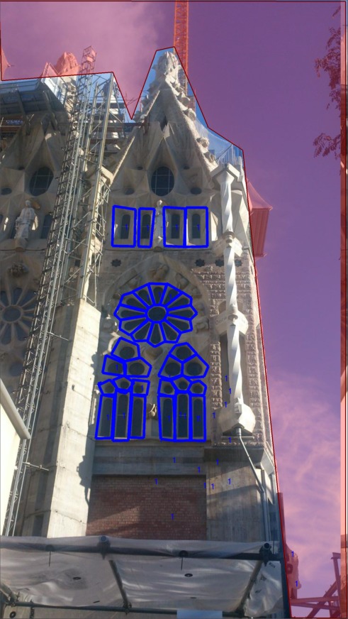
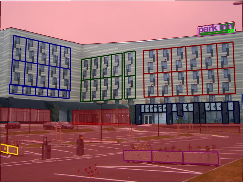
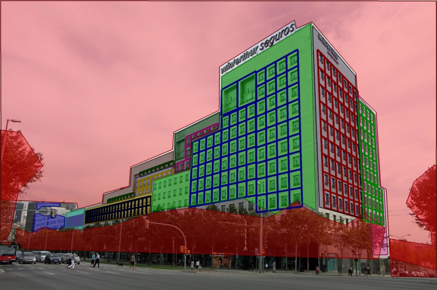
We introduce a dataset of 113 images containing from 1 to 5 scene planes with translated, reflected and rotated coplanar repeats occurring periodically or arbitrarily. The dataset includes some images from the ZuBuD database of Shao et aland the CVPR 2013 symmetry database assembled by Liu et al[Shao et al.(2003)Shao, Svoboda, and Van Gool, Liu et al.(2013)Liu, Slota, Zheng, Wu, Park, Lee, Rauschert, and Liu, Park et al.(2010)Park, Brocklehurst, Collins, and Liu]. The manual assignment of keypoints to coplanar repeat groups is infeasible since a typical image will have thousands of extracted keypoints. Direct annotation is also undesirable since setting changes of the keypoint detectors would invalidate the assignments. Instead, the annotations are designed to constrain the search for coplanar repeated keypoints, making annotations agnostic to the keypoint type. The annotations hierarchically group parallel scene planes, individual scene planes, and areas within a scene plane that cannot mutually have the same coplanar repeats, i.e. denoting distinct patterns. Clutter and non-planar surfaces are also segmented. Keypoint-level assignment to coplanar repeat groups is achieved using a RANSAC-based estimation framework which leverages the annotations to constrain the search for correspondences to choose the correct transformation type.

(a)	(b)	(c)	(d)	(e)

Figure 3: The hierarchical annotations included with the 113 image dataset. (a) translation symmetries are annotated by grids, regions that cannot share coplanar repeats are colored differently, (b) detected keypoints to vanishing line assignment, (c) groups of coplanar repeated keypoints found by annotation-assisted inference, (d) image regions (SEEDS superpixels [Van den Bergh et al.(2012)Van den Bergh, Boix, Roig, de Capitani, and Van Gool]) to vanishing line assignment, (e) and background image regions, which coplanar repeats cannot overlap.

6 Evaluation

We evaluate the proposed method against two state-of-the-art geometric multi-model fitting methods: J-Linkage and MultiRANSAC [Zuliani et al.(2005)Zuliani, Kenney, and B., Toldo and Fusiello(2008)]. Both estimators are hypothesize-and-verify variants. A model hypothesis consists of a vanishing line and tentatively grouped keypoints of similar appearance. Coplanar repeat group assignments are verified by a threshold test on the similarity measure for repeated keypoint detection proposed by Shi et al[Shi et al.(2015)Shi, Avrithis, and Jégou]. However, the rectified scale constraint defined in Eq. 2 is used in lieu of the scale kernel used by [Shi et al.(2015)Shi, Avrithis, and Jégou]. We provide the number of scene planes present in each image to MultiRANSAC.

The accuracy of rectifications constructed from vanishing lines computed from detected coplanar repeat groups are used to compare the methods. Two necessary conditions for accurate rectifications are that (i) no outliers are included in the detected coplanar repeat groups, (ii) and detected coplanar repeat groups densely cover the extents of the scene plane where there are coplanar repeat groups annotated in the dataset . Thus the rectification accuracy of coplanar repeats serves as a proxy measure for the precision and recall of coplanar repeat detection.

Projective distortion is added by rewarping a set of annotated coplanar repeats rectified by the transform computed from detected coplanar repeat groups $\hat{H}(\cdot)$ with the inverse rectification $H^{{-1}}(\cdot)$ computed from the annotated repeats. The amount of distortion is measured as the square pointwise distance between the annotated coplanar repeats and the rewarped coplanar repeats,

$$\Delta^{\hat{H}}_{\text{rms}}=\sqrt{\frac{1}{3\cdot|\mathcal{A}|}\sum_{i\in\mathcal{A}}\sum_{w=1}^{3}d^{2}(\mathbf{x}^{K}_{iw},H^{{-1}}(A^{{-1}}(\hat{H}(\mathbf{x}^{K}_{iw})))},$$ (10)

where $\mathcal{A}$ is the set of keypoint indices of the annotated coplanar repeats used to compute $H$, $A(\cdot)$ resolves the affine ambiguity between the original and rewarped annotated coplanar repeats, and $d(\cdot,\cdot)$ gives the euclidean distance between points. The set of annotated coplanar repeats that is the largest proportion of the detected coplanar repeats is used to match the rectification computed from detected coplanar repeats to a rectification computed from annotated coplanar repeats.

(a) (b) (c)

Figure 4: Evaluation. (a) CDF of rectification distortions ($\Delta_{\text{rms}}$), (b) proportion of planes rectified with less than 2 pixels of distortion in images with 1 to 5 scene planes, (c) cumulative wall time in seconds for the labeling task of energy minimization.

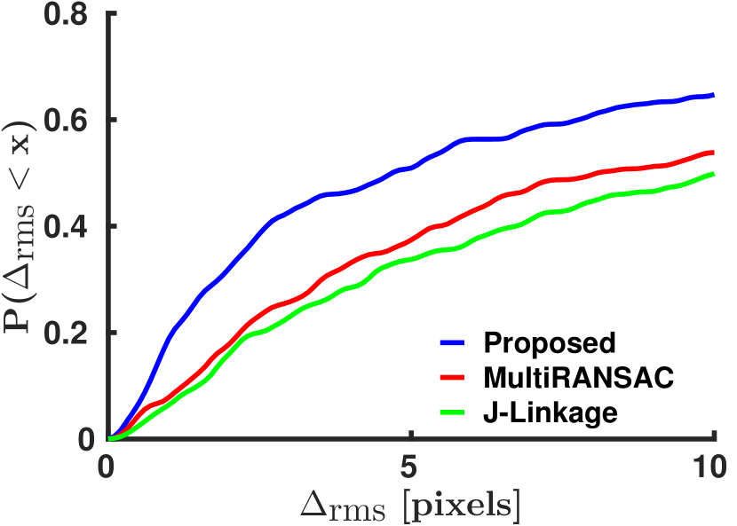
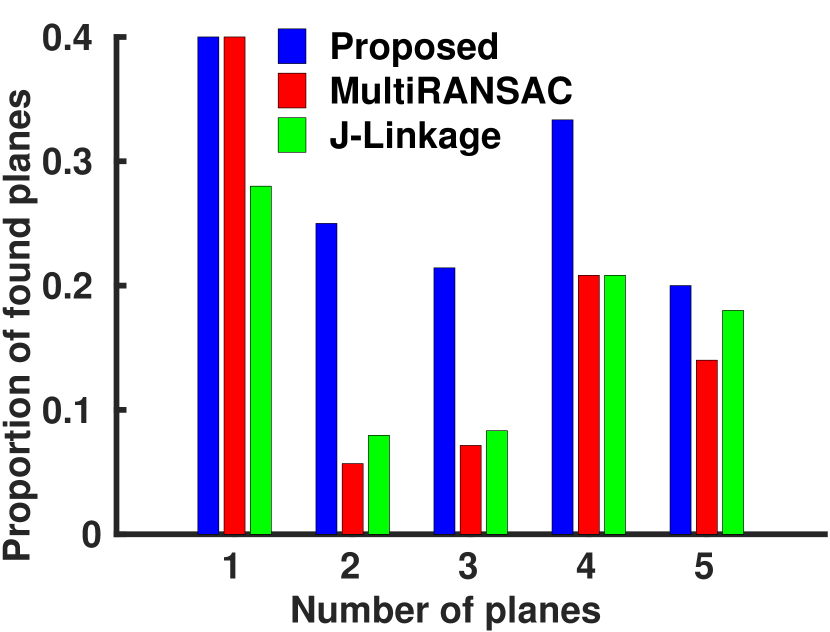
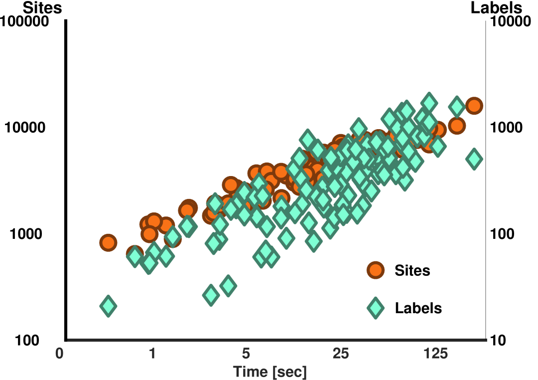
The cumulative distribution of distortions on the dataset (truncated at 10 pixels) is shown in Fig. 4a. At 1 pixel of distortion, the proposed method solves 163% more scene planes than the next best; at 2 pixels, 94% more; and at 5 pixels, which can be considered a threshold for meaningful rectification, 51% more scene planes. Fig. 4b plots the proportion of scene planes rectified with less than 2 pixels of distortion with respect to the number of scene planes in the image. Clearly the proposed method excels when there are multiple scene planes present. Fig. 4c plots the cumulative runtime of the labeling step for images as function of the number of keypoints and image regions, denoted sites, and the number of active model proposals, denoted labels. Inference ranges from under a second to 2 minutes for the largest problems in the dataset.  

7 Discussion

The proposed energy minimization formulation demonstrates a distinct increase in the quality of rectifications estimated from detected coplanar repeat groups on the evaluated dataset with respect to two state-of-the-art geometric multi-model fitting methods. The advantage can be attributed to the global scene context that is incorporated into the energy functional of the proposed method. The evaluation was performed on a new annotated dataset of images with coplanar repeats in diverse arrangements. The dataset is publicly available.

Despite a significant improvement over the baseline, the proposed method failed to solve roughly half of the dataset with less than 5 pixels of distortion. Future work will incorporate constraints specific to reflected and rotated keypoints and parallel scene lines, which would add significant geometric discrimination to the model. Learning the feature weight vector $\mathbf{w}$, which was hand tuned, could also give a significant performance boost. However, the complete annotation of coplanar repeated keypoints in an image is probably infeasible. This means structured output learning must be performed with partial annotations, which complicates the learning task considerably.

Coplanar Repeats by Energy Minimization
(Supplementary Material)

Appendix A Annotation-Assisted Repeat Grouping

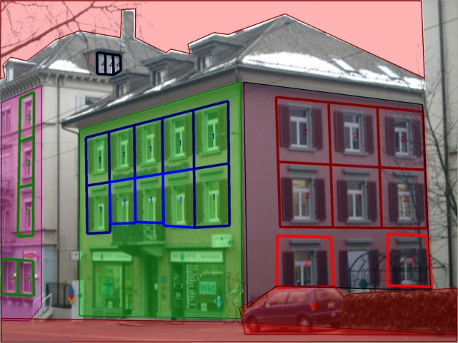
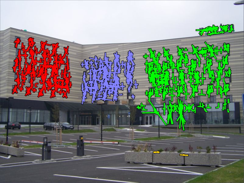
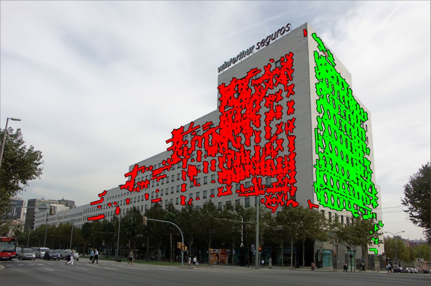
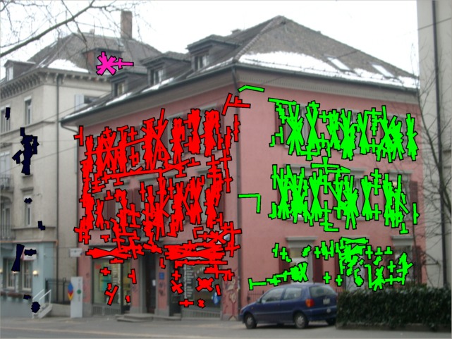
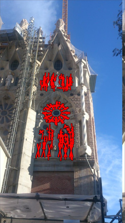
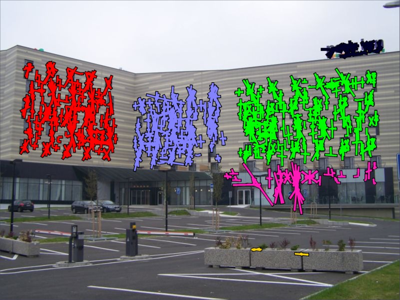
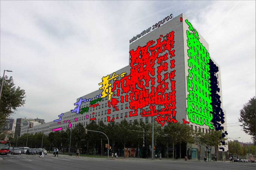
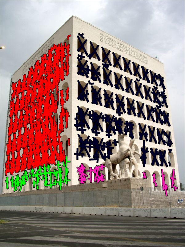
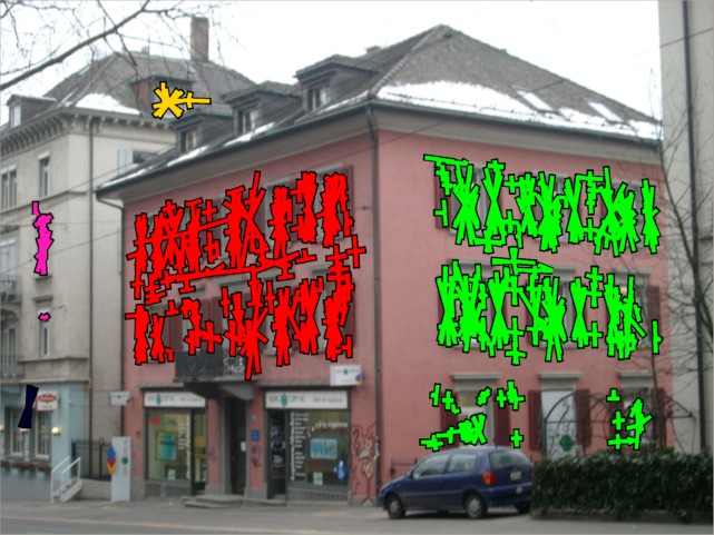
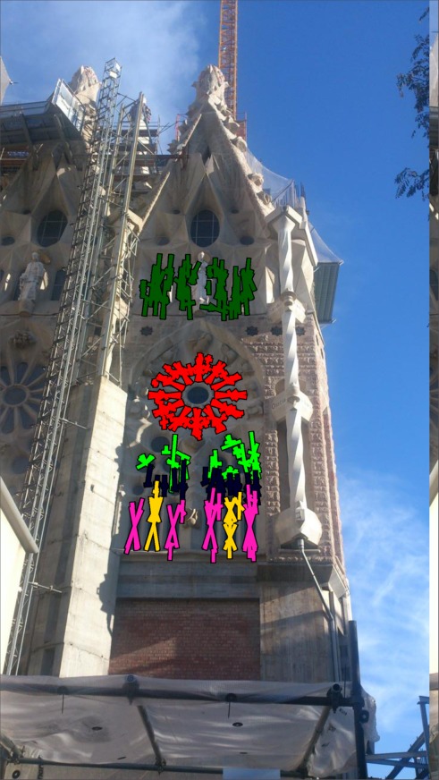
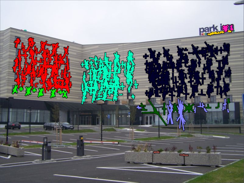
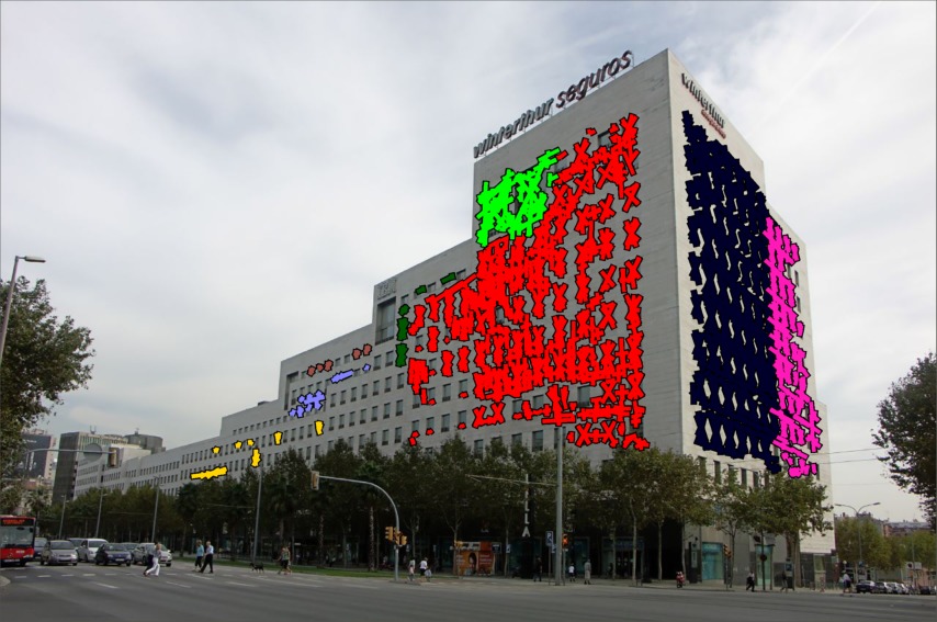
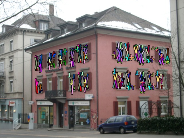
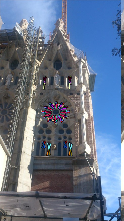
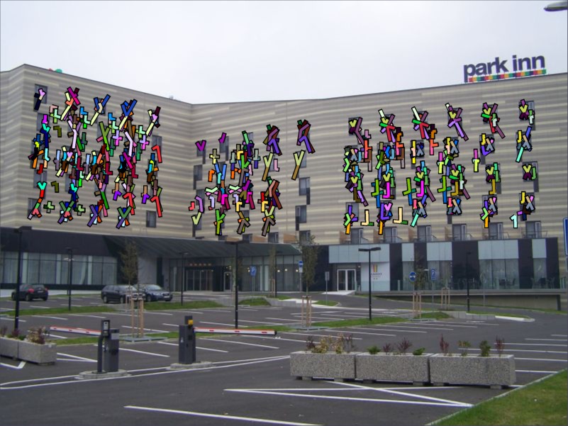
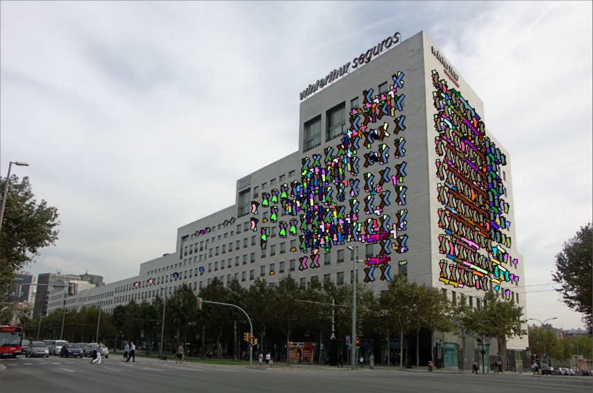
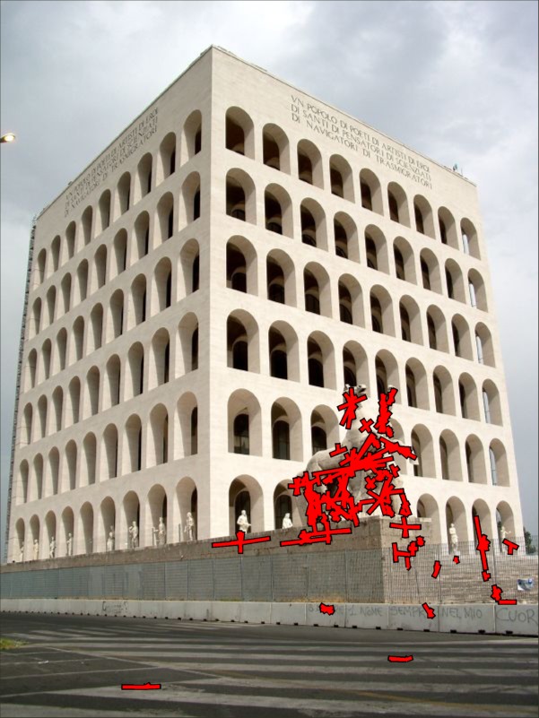
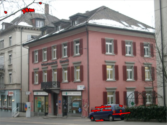
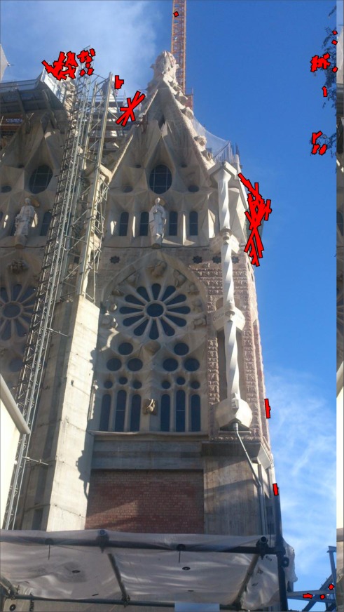
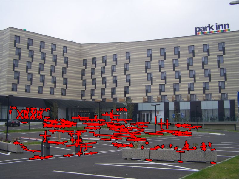
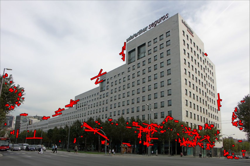
The annotations provided by the 113 image dataset referenced in the paper are discussed in detail (available at http://ptak.felk.cvut.cz/personal/prittjam/bmvc16/coplanar_repeats.tar.gz). The annotations hierarchically segment the image into parts that (i) are scene planes (ii) are the union of scene planes that share the same vanishing line (iii) contain repeated content (iv) are the union of repeated content annotations that are distinctly different from other repeated content in the remainder of the image . In particular the repeated content annotations are specific to the type of symmetry exhibited by the repeat: namely annotations for translational and rotational symmetries are provided. In addition lattices are provided for translationally symmetric periodic repeats.

Individual salient features (e.gHessian Affine Keypoints or MSERs) are not grouped or annotated, so the annotations are feature agnostic, which is preferable since settings adjustments would invalidate such annotations. Rather, the annotations are used to assist a RANSAC-based inference algorithm to establish coplanar repeat groups. The annotations constrain the search for correspondences, which gives a much higher inlier percentage among tentative groupings that are inputted to RANSAC. Since the transform type is known from the annotations, the transform with the fewest required constraints can be used, which improves the probability of proposing a transform estimated from all-inliers. The vanishing line is estimated, and, depending on the annotation tag, either a translation or rotation and translation, which maps repeats onto each pointwise. The annotations are tagged so that the correct transformation can be estimated during annotation-assisted inference.

Even with this relaxed standard of annotation, it is impossible to group repeats at their highest frequency of recurrence. Depending on the features extracted, e.g, corners of facade ornamentation may be detected, where only the windows were marked as repeated. Thus any performance evaluation must not penalize methods that correctly identify repeats that recur at higher frequencies than the annotations. Reflections and rotational symmetries, in particular, exacerbate this problem. Perhaps the most common example in the dataset are window panes, which have axial symmetry, and if square, rotational symmetry. It is not practical to annotate all such occurrences (not just restricted to windows) in a large dataset. The annotations also group oversegmetnations of the image (i.e. superpixels in this context) into contiguous components of planes, sets of parallel planes and background surface. These annotations are not currently used in the evaluation, but would be useful for learning the regularization weights in the energy function.

(a)
(b)
(c)
(d)
(e)
(f)
(g)
(h)

Figure A.1: Annotations: (a) constraints coplanar repeat grouping, (b) vanishing line assignment, (c) plane assignment, (d) mutually distinct repeated content, (e) coplanar repeats found by annotation-assisted inference, (f) features on the background surface, (g) vanishing line assignment for regions, (h) regions on the background surface.

References

- [Arandjelović and Zisserman(2012)] R. Arandjelović and A. Zisserman. Three things everyone should know to improve object retrieval. In CVPR, 2012.
- [Boykov et al.(2001)Boykov, Veksler, and Zabih] Y. Boykov, O. Veksler, and R. Zabih. Fast approximate energy minimization via graph cuts. PAMI, 23(11):1222–1239, 2001.
- [Chum and Matas(2010)] O. Chum and J. Matas. Planar affine rectification from change of scale. In ACCV, 2010.
- [Delong et al.(2012)Delong, Osokin, Isack, and Boykov] A. Delong, A. Osokin, H. N. Isack, and Y. Boykov. Fast approximate energy minimization with label costs. IJCV, 96:1–27, 2012.
- [Isack and Boykov(2012)] H. Isack and Y. Boykov. Energy-based geometric multi-model fitting. IJCV, 97(2):123–147, 2012.
- [Kolmogorov and Zabih(2004)] V. Kolmogorov and R. Zabih. What energy functions can be minimized via graph cuts. PAMI, 26:65–81, 2004.
- [Liebowitz and Zisserman(1998)] D. Liebowitz and A. Zisserman. Metric rectification for perspective images of planes. In CVPR, 1998.
- [Liu et al.(2013)Liu, Slota, Zheng, Wu, Park, Lee, Rauschert, and Liu] J. Liu, G. Slota, G. Zheng, Z. Wu, M. Park, S. Lee, I. Rauschert, and Y. Liu. Symmetry detection from real world images competition 2013: Summary and results. In CVPR Workshop, 2013.
- [Lowe(2004)] D. Lowe. Distinctive image features from scale-invariant keypoints. IJCV, 60(2):91–110, 2004.
- [Matas et al.(2002a)Matas, Chum, Urban, and Pajdla] J. Matas, O. Chum, M. Urban, and T. Pajdla. Robust wide baseline stereo from maximally stable extremal regions. In BMVC, 2002a.
- [Matas et al.(2002b)Matas, Obdržálek, and Chum] J. Matas, S. Obdržálek, and O. Chum. Local affine frames for wide-baseline stereo. In ICPR, 2002b.
- [Mikolajczyk and Schmid(2004)] K. Mikolajczyk and C. Schmid. Scale & affine invariant interest point detectors. IJCV, 1(60):63–86, 2004.
- [Obdržálek and Matas(2002)] Š. Obdržálek and J. Matas. Object recognition using local affine frames on distinguished regions. In BMVC, 2002.
- [Park et al.(2009)Park, Brocklehurst, Collins, and Liu] M. Park, K. Brocklehurst, R. Collins, and Y. Liu. Deformed lattice detection in real-world images using mean-shift belief propagation. PAMI, 2009.
- [Park et al.(2010)Park, Brocklehurst, Collins, and Liu] M. Park, K. Brocklehurst, R. T Collins, and Y. Liu. Translation-symmetry-based perceptual grouping with applications to urban scenes. In ACCV. 2010.
- [Pritts et al.(2014)Pritts, Chum, and Matas] J. Pritts, O. Chum, and J. Matas. Detection, rectification and segmentation of coplanar repeated patterns. In CVPR, 2014.
- [Rother et al.(2004)Rother, Kolmogorov, and Blake] C. Rother, V. Kolmogorov, and A. Blake. Grabcut: Interactive foreground extraction using iterated graph cuts. ACM Trans. Graph., 23(3):309–314, August 2004.
- [Schaffalitzky and Zisserman(1998)] F. Schaffalitzky and A. Zisserman. Geometric grouping of repeated elements within images. In BMVC, 1998.
- [Shao et al.(2003)Shao, Svoboda, and Van Gool] H. Shao, T. Svoboda, and L. Van Gool. Zubud-zurich buildings database for image based recognition. Computer Vision Lab, Swiss Federal Institute of Technology, Switzerland, Tech. Rep, 260, 2003.
- [Shi et al.(2015)Shi, Avrithis, and Jégou] M. Shi, Y. Avrithis, and H. Jégou. Early burst detection for memory-efficient image retrieval. In CVPR, 2015.
- [Toldo and Fusiello(2008)] R. Toldo and A. Fusiello. Robust multiple structures estimation with j-linkage. In ECCV, 2008.
- [Tuytelaars et al.(2003)Tuytelaars, Turina, and Van Gool] T. Tuytelaars, A. Turina, and L. Van Gool. Noncombinatorial detection of regular repetitions under perspective skew. PAMI, 25(4):418–432, April 2003.
- [Van den Bergh et al.(2012)Van den Bergh, Boix, Roig, de Capitani, and Van Gool] M. Van den Bergh, X. Boix, G. Roig, B. de Capitani, and L. Van Gool. Seeds: Superpixels extracted via energy-driven sampling. In ECCV, 2012.
- [Wu et al.(2010)Wu, Frahm, and Pollefeys] C. Wu, J. Frahm, and M. Pollefeys. Detecting large repetitive structures with salient boundaries. In ECCV, 2010.
- [Zuliani et al.(2005)Zuliani, Kenney, and B.] M. Zuliani, C. Kenney, and Manjunath B. The multiransac algorithm and its application to detect planar homographies. In ICIP, 2005.