The C2HDM revisited

Abstract

The complex two-Higgs doublet model is one of the simplest ways to extend the scalar sector of the Standard Model to include a new source of CP-violation. The model has been used as a benchmark model to search for CP-violation at the LHC and as a possible explanation for the matter-antimatter asymmetry of the Universe. In this work, we re-analyse in full detail the softly broken $\mathbb{Z}_{2}$ symmetric complex two-Higgs doublet model (C2HDM). We provide the code C2HDM_HDECAY implementing the C2HDM in the well-known HDECAY program which calculates the decay widths including the state-of-the-art higher order QCD corrections and the relevant off-shell decays. Using C2HDM_HDECAY together with the most relevant theoretical and experimental constraints, including electric dipole moments (EDMs), we review the parameter space of the model and discuss its phenomenology. In particular, we find cases where large CP-odd couplings to fermions are still allowed and provide benchmark points for these scenarios. We examine the prospects of discovering CP-violation at the LHC and show how theoretically motivated measures of CP-violation correlate with observables.

1 Introduction

After the discovery of the Higgs boson by the ATLAS Aad:2012tfa and CMS Chatrchyan:2012ufa collaborations the Large Hadron Collider (LHC) has now entered the Run 2 stage with a 13 TeV centre-of-mass energy. The search for physics beyond the Standard Model (BSM) is now the main goal of the LHC experiments. An important motivation of BSM physics is to provide new sources of CP-violation to fulfil the three Sakharov criteria for baryogenesis Sakharov:1967dj . The simplest extension of the scalar sector that can provide a new source of CP-violation, the two-Higgs doublet model (2HDM) Lee:1973iz , can address this issue. Reviews of the 2HDM can be found in Gunion:1989we ; Branco:2011iw ; Ivanov:2017dad .

One of the simplest ways of extending the SM with a CP-violating scalar sector without the addition of new fermions is to add a scalar doublet to the SM content and build a 2HDM softly broken $\mathbb{Z}_{2}$ symmetric potential with two complex parameters. This model, now known as C2HDM, was first discussed in Ginzburg:2002wt and has only one independent CP-phase and a simple limit leading to its CP-conserving version. The model has been the subject of many studies Khater:2003wq ; ElKaffas:2007rq ; Grzadkowski:2009iz ; Arhrib:2010ju ; Barroso:2012wz ; Inoue:2014nva ; Cheung:2014oaa ; Fontes:2014xva ; Fontes:2015mea ; Chen:2015gaa . More recently a comparison with a number of other extensions of the SM was performed Muhlleitner:2017dkd . The NLO QCD corrections to double Higgs decays were also recently calculated in Grober:2017gut .

One of the primary goals of the LHC Run 2 is to look for new particles but also to probe the CP parity of both the discovered Higgs boson and of any further scalars yet undiscovered. Due to its simplicity, the C2HDM is the ideal benchmark model to test the CP quantum numbers of the scalars at the LHC. The CP-nature of the scalars, in their Yukawa couplings, can be probed directly either in the production or the decays of the Higgs bosons. In this case, it is the relation between the scalar and the pseudoscalar components in the Yukawa couplings that is probed. Some examples of the use of asymmetries to probe the CP-nature of the Higgs boson in the top Yukawa coupling were discussed in Gunion:1996xu ; Boudjema:2015nda ; AmorDosSantos:2017ayi while the decays of the tau leptons were used to probe the tau Yukawa coupling Berge:2008wi ; Berge:2008dr ; Berge:2011ij ; Berge:2014sra ; Berge:2015nua . Correlations in the momentum distributions of leptons produced in the decays of the Higgs boson to gauge bosons were used to probe the CP-nature of the Higgs boson couplings to gauge bosons Choi:2002jk ; Buszello:2002uu ; Godbole:2007cn by the ATLAS Aad:2015mxa and CMS Khachatryan:2016tnr collaborations. The most general CP-violating $HVV$ coupling was used, and limits were set on the anomalous couplings. However, the C2HDM has SM-like couplings to the gauge bosons - it is just the SM coupling multiplied by a number. The anomalous couplings only appear at loop level and are consequently very small. Therefore, in this model, only the Yukawa couplings can lead to direct observations of CP-violation.

There are, however, other ways to probe CP-violation using only inclusive observables. As proposed in Branco:1999fs ; Fontes:2015xva several combinations of three simultaneously observed Higgs decay modes can constitute an undoubtable sign of CP-violation. In a CP-conserving model, a decay of the type $H_{i}\rightarrow H_{j}Z$ would imply opposite CP parities for $H_{i}$ and $H_{j}$. In a renormalisable theory, a Higgs boson decaying to a pair of gauge bosons has to be CP-even.

Hence, the combination of the decays $H_{i}\rightarrow H_{j}Z$, $H_{i}\rightarrow ZZ$ and $H_{j}\rightarrow ZZ$ is a clear sign of CP-violation. In Fontes:2015xva seven classes of decays were defined, some of which signal CP-violation for any extension of the SM, while others are not possible in a CP-conserving 2HDM but can occur in the C2HDM or even in models with 3 CP-even states. An example of the latter is $H_{i}\to ZZ$ (with $i=1,2,3$) that could signal CP-violation but could also happen in a model with at least 3 CP-even states. In some extensions of the SM, even the ones with just two extra scalars, as is the case of the SM plus a complex singlet, all $H_{i}$ are CP-even, and therefore the decays $H_{i}\to ZZ$ all happen at tree-level. From the above classes, we are especially interested in the ones that include the already observed decay of the SM-like Higgs boson, denoted by $h_{125}$, to gauge bosons, $h_{125}\to ZZ$. Furthermore, decays of the type $H_{i}\to ZZ$ and $H_{i}\to H_{j}Z$ were the subject of searches during Run 1 which will proceed during Run 2. Therefore, if a new Higgs boson is observed in the final states with gauge bosons and also in the final state $h_{125}Z$ the scalar sector is immediately established to be CP-violating.

In the C2HDM there is only one independent CP-violating phase. Hence, the only three basis-invariant quantities that signal CP-violation Lavoura:1994fv ; Botella:1994cs are all related and proportional to that phase. In this work, we are interested in finding a relation between the production rates in each of the CP-violating classes and variables that signal CP-violation. Therefore we will test a number of variables in the most interesting classes that include the already observed $h_{125}\to ZZ$. Finally, decays of the type $H_{j}\to H_{i}h_{125}$ can only happen in very specific models and searches for this particular channel are important and should be a priority for Run 2.

The LHC Run 2 will bring increasing precision in the measurement of Higgs production and decay rates. The ATLAS and CMS collaborations have started testing new models such as the singlet extension of the SM and the CP-conserving 2HDM. To probe other extensions of the SM new tools are needed to increase the precision both in the Higgs production rates and also in the Higgs decay widths. Hence, one of the main purposes of this work is the release of the C2HDM_HDECAY code, an implementation of the C2HDM in HDECAY v6.51 Djouadi:1997yw ; Butterworth:2010ym . The code is entirely self-contained, and the widths include the most important state-of-the-art higher order QCD corrections and the relevant off-shell decays.

The paper is organised as follows. In section 2 we describe the model and in section  3 we discuss the parameter space of the model given the most relevant theoretical and up to date experimental constraints. We identify situations where $h_{125}$ could have remarkable properties and give benchmark points for these scenarios. Namely, situations where its couplings to fermions have a large CP-odd component and the possibilities that $h_{125}$ is the heaviest of the three scalars in the C2HDM. In section 4, we discuss the production rates of processes that constitute classes of CP-violating decays and relate them with a number of variables that can probe CP-violation. In section 5 we discuss Higgs-to-Higgs decays in the framework of the C2HDM. Our conclusions are presented in section 6. In appendix A we write the Feynman rules for the C2HDM in the unitary gauge. In appendix B we describe the C2HDM_HDECAY code.

2 The complex two-Higgs doublet model

The version of the complex two-Higgs doublet model we discuss in this work has an explicitly CP-violating scalar potential, with a softly broken $\mathbb{Z}_{2}$ symmetry $\Phi_{1}\rightarrow\Phi_{1},\Phi_{2}\rightarrow-\Phi_{2}$ written as

$$V = m_{11}^{2}|\Phi_{1}|^{2}+m_{22}^{2}|\Phi_{2}|^{2}-\left(m_{12}^{2}\,\Phi_{1}^{\dagger}\Phi_{2}+h.c.\right)+\frac{\lambda_{1}}{2}(\Phi_{1}^{\dagger}\Phi_{1})^{2}+\frac{\lambda_{2}}{2}(\Phi_{2}^{\dagger}\Phi_{2})^{2}$$ (2.1)

$$+\lambda_{3}(\Phi_{1}^{\dagger}\Phi_{1})(\Phi_{2}^{\dagger}\Phi_{2})+\lambda_{4}(\Phi_{1}^{\dagger}\Phi_{2})(\Phi_{2}^{\dagger}\Phi_{1})+\left[\frac{\lambda_{5}}{2}(\Phi_{1}^{\dagger}\Phi_{2})^{2}+h.c.\right]\;.$$

Due to the hermiticity of the Lagrangian, all couplings are real except for $m_{12}^{2}$ and $\lambda_{5}$. We write each of the doublets $\Phi_{i}$ $(i=1,2)$ as an expansion around the real vacuum expectation values (VEVs) $v_{1}$ and $v_{2}$, in terms of the charged complex fields ($\phi_{i}^{+}$) and the real neutral fields ($\rho_{i}$ and $\eta_{i}$). The doublets then read

$$\Phi_{1}=\left(\begin{array}[]{c}\phi_{1}^{+}\\ \frac{v_{1}+\rho_{1}+i\eta_{1}}{\sqrt{2}}\end{array}\right)\qquad\mbox{and}\qquad\Phi_{2}=\left(\begin{array}[]{c}\phi_{2}^{+}\\ \frac{v_{2}+\rho_{2}+i\eta_{2}}{\sqrt{2}}\end{array}\right)\;.$$ (2.6)

The minimum conditions for the potential are

$$m_{11}^{2}v_{1}+\frac{\lambda_{1}}{2}v_{1}^{3}+\frac{\lambda_{345}}{2}v_{1}v_{2}^{2} = \textrm{Re}\left(m_{12}^{2}\right)v_{2}\;,$$ (2.7)

$$m_{22}^{2}v_{2}+\frac{\lambda_{2}}{2}v_{2}^{3}+\frac{\lambda_{345}}{2}v_{1}^{2}v_{2} = \textrm{Re}\left(m_{12}^{2}\right)v_{1}\;,$$ (2.8)

$$2\,\mbox{Im}(m_{12}^{2}) = v_{1}v_{2}\mbox{Im}(\lambda_{5})\;,$$ (2.9)

where we have introduced

$$\lambda_{345}\equiv\lambda_{3}+\lambda_{4}+\mbox{Re}(\lambda_{5})\;.$$ (2.10)

We define two CP-violating phases $\phi(m_{12}^{2})$ and $\phi(\lambda_{5})$ as

$$m_{12}^{2}=|m_{12}^{2}|\,e^{i\,\phi(m_{12}^{2})}\,,\qquad\qquad\lambda_{5}=|\lambda_{5}|\,e^{i\,\phi(\lambda_{5})}\,.$$ (2.11)

Equation (2.9) shows us that these two phases are not independent. We can re-write eq. (2.9) as

$$2\text{Re}\!{\,(m_{12}^{2})}\,\tan\phi(m_{12}^{2})=v_{1}v_{2}\,\text{Re}\!{\,(\lambda_{5})}\,\tan\phi(\lambda_{5})\,.$$ (2.12)

We choose both vacuum expectation values $v_{1}$ and $v_{2}$ to be real which together with the condition $\phi(\lambda_{5})\neq 2\,\phi(m_{12}^{2})$ Ginzburg:2002wt ensures that the two phases cannot be removed simultaneously. Otherwise we are in the CP-conserving limit of the model.

The Higgs basis Lavoura:1994fv ; Botella:1994cs $\{{\cal H}_{1},{\cal H}_{2}\}$ is defined by the rotation

$$\left(\begin{array}[]{c}{\cal H}_{1}\\ {\cal H}_{2}\end{array}\right)=R^{T}_{H}\left(\begin{array}[]{c}\Phi_{1}\\ \Phi_{2}\end{array}\right)\equiv\left(\begin{array}[]{cc}c_{\beta}&s_{\beta}\\ -s_{\beta}&c_{\beta}\end{array}\right)\left(\begin{array}[]{c}\Phi_{1}\\ \Phi_{2}\end{array}\right)\;,$$ (2.21)

with

$$\tan\beta\equiv\frac{v_{2}}{v_{1}}\;,$$ (2.22)

and the doublets in the Higgs basis are written as

$${\cal H}_{1}=\left(\begin{array}[]{c}G^{\pm}\\ \frac{1}{\sqrt{2}}(v+H^{0}+iG^{0})\end{array}\right)\quad\mbox{and}\qquad{\cal H}_{2}=\left(\begin{array}[]{c}H^{\pm}\\ \frac{1}{\sqrt{2}}(R_{2}+iI_{2})\end{array}\right)\;.$$ (2.27)

The SM VEV $v=\sqrt{v_{1}^{2}+v_{2}^{2}}$ along with the Goldstone bosons $G^{\pm}$ and $G^{0}$ is now in ${\cal H}_{1}$, while the charged Higgs mass eigenstates $H^{\pm}$ are in ${\cal H}_{2}$. The neutral Higgs mass eigenstates $H_{i}$ ($i=1,2,3$) are obtained from the neutral components of the C2HDM basis, $\rho_{1}$, $\rho_{2}$ and $\rho_{3}\equiv I_{2}$, via the rotation

$$\left(\begin{array}[]{c}H_{1}\\ H_{2}\\ H_{3}\end{array}\right)=R\left(\begin{array}[]{c}\rho_{1}\\ \rho_{2}\\ \rho_{3}\end{array}\right)\;.$$ (2.34)

The model has three neutral particles with no definite CP quantum numbers, $H_{1}$, $H_{2}$ and $H_{3}$, and two charged scalars $H^{\pm}$. The mass matrix of the neutral scalar states

$$({\cal M}^{2})_{ij}=\left\langle\frac{\partial^{2}V}{\partial\rho_{i}\partial\rho_{j}}\right\rangle\;,$$ (2.35)

is diagonalised via the orthogonal matrix $R$ ElKaffas:2007rq . That is,

$$R{\cal M}^{2}R^{T}=\mbox{diag}(m_{H_{1}}^{2},m_{H_{2}}^{2},m_{H_{3}}^{2})\;,$$ (2.36)

for which we choose the form

$$R=\left(\begin{array}[]{ccc}c_{1}c_{2}&s_{1}c_{2}&s_{2}\\ -(c_{1}s_{2}s_{3}+s_{1}c_{3})&c_{1}c_{3}-s_{1}s_{2}s_{3}&c_{2}s_{3}\\ -c_{1}s_{2}c_{3}+s_{1}s_{3}&-(c_{1}s_{3}+s_{1}s_{2}c_{3})&c_{2}c_{3}\end{array}\right)\,,$$ (2.37)

with $s_{i}=\sin{\alpha_{i}}$, $c_{i}=\cos{\alpha_{i}}$ ($i=1,2,3$), and

$$-\pi/2<\alpha_{1}\leq\pi/2,\hskip 21.52771pt-\pi/2<\alpha_{2}\leq\pi/2,\hskip 21.52771pt-\pi/2<\alpha_{3}\leq\pi/2.$$ (2.38)

The Higgs boson masses are ordered such that $m_{H_{1}}\leq m_{H_{2}}\leq m_{H_{3}}$.

Note that the mass basis and the Higgs basis are related through

$$\left(\begin{array}[]{c}H_{1}\\ H_{2}\\ H_{3}\end{array}\right)=T^{T}\left(\begin{array}[]{c}H^{0}\\ R_{2}\\ I_{2}\end{array}\right)\;,$$ (2.45)

where the matrix $T$ used in ref. Branco:2011iw for the expression of the oblique radiative corrections is defined as

$$T^{T}=R\widetilde{R}_{H}$$ (2.46)

and $\widetilde{R}_{H}$ is given by

$$\widetilde{R}_{H}=\left(\begin{array}[]{cc}R_{H}&0\\ 0&1\end{array}\right)\;.$$ (2.49)

Our choice of the 9 independent parameters of the C2HDM is: $v=\sqrt{v_{1}^{2}+v_{2}^{2}}$, $\tan\beta$, $m_{H^{\pm}}$, $\alpha_{1}$, $\alpha_{2}$, $\alpha_{3}$, $m_{H_{1}}$, $m_{H_{2}}$, and $\textrm{Re}(m_{12}^{2})$. With this choice, the mass of the heaviest neutral scalar is a dependent parameter, given by

$$m_{H_{3}}^{2}=\frac{m_{H_{1}}^{2}\,R_{13}(R_{12}\tan{\beta}-R_{11})+m_{H_{2}}^{2}\ R_{23}(R_{22}\tan{\beta}-R_{21})}{R_{33}(R_{31}-R_{32}\tan{\beta})},$$ (2.50)

and the parameter space points will have to comply with $m_{H_{3}}>m_{H_{2}}$.

We will briefly describe here the couplings of the Higgs bosons with the remaining SM fields. A longer list is provided in appendix A, and the full set is contained in the web page C2HDM_FR . The Higgs couplings to the massive gauge bosons $V=W,Z$ are given by

$$i\,g_{\mu\nu}\,c(H_{i}VV)\,g_{H^{\text{S}M}VV}\;,$$ (2.51)

where $g_{H^{\text{S}M}VV}$ denotes the corresponding SM Higgs coupling, given by

$$g_{H^{\text{S}M}VV}=\left\{\begin{array}[]{c}gM_{W}\qquad\qquad\quad V=W\\ gM_{Z}/\cos\theta_{W}\qquad V=Z\end{array}\right.\qquad$$ (2.54)

where $g$ is the $SU(2)$ gauge coupling and $\theta_{W}$ is the Weinberg angle. The effective couplings can be written as

$$c(H_{i}VV)=T_{1i}=c_{\beta}R_{i1}+s_{\beta}R_{i2}\;.$$ (2.55)

The Yukawa sector is built by extending the $\mathbb{Z}_{2}$ symmetry to the fermion fields such that flavour changing neutral currents (FCNC) are absent at tree-level Glashow:1976nt ; Paschos:1976ay . There are four possible $\mathbb{Z}_{2}$ charge assignments and therefore four different types of 2HDMs described in table 1.

	$u$-type	$d$-type	leptons
Type I	$\Phi_{2}$	$\Phi_{2}$	$\Phi_{2}$
Type II	$\Phi_{2}$	$\Phi_{1}$	$\Phi_{1}$
Lepton-Specific	$\Phi_{2}$	$\Phi_{2}$	$\Phi_{1}$
Flipped	$\Phi_{2}$	$\Phi_{1}$	$\Phi_{2}$

Table 1: The four Yukawa types of the softly broken $\mathbb{Z}_{2}$-symmetric 2HDM.

The Yukawa Lagrangian has the form

$${\cal L}_{Y}=-\sum_{i=1}^{3}\frac{m_{f}}{v}\bar{\psi}_{f}\left[c^{e}(H_{i}ff)+ic^{o}(H_{i}ff)\gamma_{5}\right]\psi_{f}H_{i}\;,$$ (2.56)

where $\psi_{f}$ denote the fermion fields with mass $m_{f}$. The coefficients of the CP-even and of the CP-odd part of the Yukawa coupling, $c^{e}(H_{i}ff)$ and $c^{o}(H_{i}ff)$, are presented in table 2.

	$u$-type	$d$-type	leptons
Type I	$\frac{R_{i2}}{s_{\beta}}-i\frac{R_{i3}}{t_{\beta}}\gamma_{5}$	$\frac{R_{i2}}{s_{\beta}}+i\frac{R_{i3}}{t_{\beta}}\gamma_{5}$	$\frac{R_{i2}}{s_{\beta}}+i\frac{R_{i3}}{t_{\beta}}\gamma_{5}$
Type II	$\frac{R_{i2}}{s_{\beta}}-i\frac{R_{i3}}{t_{\beta}}\gamma_{5}$	$\frac{R_{i1}}{c_{\beta}}-it_{\beta}R_{i3}\gamma_{5}$	$\frac{R_{i1}}{c_{\beta}}-it_{\beta}R_{i3}\gamma_{5}$
Lepton-Specific	$\frac{R_{i2}}{s_{\beta}}-i\frac{R_{i3}}{t_{\beta}}\gamma_{5}$	$\frac{R_{i2}}{s_{\beta}}+i\frac{R_{i3}}{t_{\beta}}\gamma_{5}$	$\frac{R_{i1}}{c_{\beta}}-it_{\beta}R_{i3}\gamma_{5}$
Flipped	$\frac{R_{i2}}{s_{\beta}}-i\frac{R_{i3}}{t_{\beta}}\gamma_{5}$	$\frac{R_{i1}}{c_{\beta}}-it_{\beta}R_{i3}\gamma_{5}$	$\frac{R_{i2}}{s_{\beta}}+i\frac{R_{i3}}{t_{\beta}}\gamma_{5}$

Table 2: Yukawa couplings of the Higgs bosons $H_{i}$ in the C2HDM, divided by the corresponding SM Higgs couplings. The expressions correspond to $[c^{e}(H_{i}ff)+ic^{o}(H_{i}ff)\gamma_{5}]$ from eq. (2.56).

These couplings were implemented in the code HDECAY Djouadi:1997yw ; Butterworth:2010ym which provides all Higgs decay widths and branching ratios including the state-of-the-art higher order QCD corrections and off-shell decays. The description of the new C2HDM_HDECAY code is presented in appendix B.

3 The C2HDM Parameter Space

3.1 Experimental and Theoretical Restrictions

The C2HDM was implemented as a model class in ScannerS Coimbra:2013qq ; ScannerS . The most relevant theoretical and experimental bounds are either built in the code or acessible via interfaces with other codes. We have imposed all available constraints on the model and performed a parameter scan. The resulting viable points are the basis for our phenomenological analyses for the LHC Run 2.

The theoretical bounds included in ScannerS are boundness from below and perturbative unitarity Kanemura:1993hm ; Akeroyd:2000wc ; Ginzburg:2003fe . Contrary to the SM, in the 2HDM coexisting minima can occur at tree-level. Therefore we also force the minimum to be global Ivanov:2015nea , precluding the possibility of vacuum decay. The points generated comply with electroweak precision measurements, making use of the oblique parameters $S$, $T$ and $U$ Branco:2011iw . We ask for a $2\sigma$ compatibility of $S$, $T$ and $U$ with the SM fit presented in Baak:2014ora . The full correlation among these parameters is taken into account.

The charged sector of the C2HDM has exactly the same couplings as in the 2HDM. Therefore, the exclusion bounds on the $m_{H^{\pm}}-t_{\beta}$ plane can be imported from the 2HDM. The most constraining bounds on this plane come from the measurements of $B\to X_{s}\gamma$ Deschamps:2009rh ; Mahmoudi:2009zx ; Hermann:2012fc ; Misiak:2015xwa ; Misiak:2017bgg . The latest $2\sigma$ bounds on this plane were obtained in Misiak:2017bgg and force the charged Higgs mass to be $m_{H^{\pm}}>580\mbox{ GeV}$ for models Type II and Flipped, almost independently of $\tan\beta$. Due to the structure of the charged Higgs couplings to fermions, in models Type I and Lepton-Specific the bound has a strong dependence on $\tan\beta$. In fact, for $\tan\beta\approx 1$ the bound is about $400\mbox{ GeV}$ while the LEP bound derived from $e^{+}e^{-}\to H^{+}H^{-}$ Abbiendi:2013hk (approximately $100\mbox{ GeV}$) is recovered for $\tan\beta\approx 1.8$. We further apply the flavour constraints from $R_{b}$ Haber:1999zh ; Deschamps:2009rh . All the constraints are checked as $2\sigma$ exclusion bounds on the $m_{H^{\pm}}-t_{\beta}$ plane.

The SM-like Higgs boson is denoted by $h_{125}$ and has a mass of $m_{h_{125}}=125.09\;\mbox{GeV}$ Aad:2015zhl . We exclude points of the parameter space with the discovered Higgs signal built by two nearly degenerate Higgs boson states by forcing the non-SM scalar masses to be outside the mass window $m_{h_{125}}\pm 5$ GeV. Compatibility with the exclusion bounds from Higgs searches is checked with the HiggsBounds code Bechtle:2008jh ; Bechtle:2011sb ; Bechtle:2013wla , while the individual signal strengths for the SM-like Higgs boson are forced to be within $2\sigma$ of the fits presented in Khachatryan:2016vau . Branching ratios and decay widths of all Higgs bosons are calculated with the C2HDM_HDECAY code, described in appendix B, which is an implementation of the C2HDM model into HDECAY v6.51. The code has state-of-the-art QCD corrections and off-shell decays, but off-shell decays of one scalar into two are not included. The Higgs boson production cross sections via gluon fusion ($ggF$) and $b$-quark fusion ($bbF$) are calculated with SusHiv1.6.0 Harlander:2012pb ; Harlander:2016hcx , which is interfaced with ScannerS, at next-to-next-to-leading order (NNLO) QCD. As the neutral scalars have no definite CP, we need to combine the CP-odd and the CP-even contributions by summing them incoherently. That is, $\mu_{F}$ is given by

$$\mu_{F}=\frac{\sigma^{\text{even}}_{\text{C2HDM}}(ggF)+\sigma^{\text{even}}_{\text{C2HDM}}(bbF)+\sigma^{\text{odd}}_{\text{C2HDM}}(ggF)+\sigma^{\text{odd}}_{\text{C2HDM}}(bbF)}{\sigma^{\text{even}}_{\text{SM}}(ggF)}\;,$$ (3.57)

where in the denominator we neglected the $bbF$ cross section since in the SM it is much smaller than gluon fusion production. The CP-even Higgs production cross sections in association with a vector boson ($VH$) and in vector boson fusion ($VBF$) give rise to the normalised production strengths

$$\mu_{V}=\frac{\sigma^{\text{even}}_{\text{C2HDM}}(VBF)}{\sigma^{\text{even}}_{\text{SM}}(VBF)}=\frac{\sigma^{\text{even}}_{\text{C2HDM}}(VH)}{\sigma^{\text{even}}_{\text{SM}}(VH)}=c^{2}(H_{i}VV)\;,$$ (3.58)

because QCD corrections cancel at NLO. The effective couplings are defined in eq. (2.51).

Both CP-even and CP-odd components contribute to the cross sections for associated production with fermions. As these have different QCD corrections Hafliger:2005aj , we opted for using leading order production cross sections, and write the strengths as

$$\mu_{\text{assoc}}=\frac{\sigma_{\text{C2HDM}}(ffH_{i})}{\sigma_{\text{SM}}(ffH)}=c^{e}(H_{i}ff)^{2}+c^{o}(H_{i}ff)^{2}\;,$$ (3.59)

with the coupling coefficients defined in eq. (2.56). We then use HiggsBounds via the ScannerS interface to ensure compatibility at $2\sigma$ with all available collider data. Regarding the SM-like Higgs boson, the parameter space is forced to be in agreement with the fit results from Khachatryan:2016vau . That is, the values

$$\frac{\mu_{F}}{\mu_{V}}\;,\quad\mu_{\gamma\gamma}\;,\quad\mu_{ZZ}\;,\quad\mu_{WW}\;,\quad\mu_{\tau\tau}\;,\quad\mu_{bb}\;,$$ (3.60)

given in Khachatryan:2016vau , with $\mu_{xx}$ defined as

$$\mu_{xx}=\mu_{F}\,\frac{\mbox{BR}_{\text{C2HDM}}(H_{i}\to xx)}{\mbox{BR}_{\text{SM}}(H^{SM}\to xx)}$$ (3.61)

for $H_{i}\equiv h_{125}$, are within $2\sigma$ of the fitted experimental values. Here $H^{SM}$ denotes the SM Higgs boson with a mass of 125.09 GeV. As the C2HDM preserves custodial symmetry, $\mu_{ZZ}=\mu_{WW}\equiv\mu_{VV}$, we can combine the lower $2\sigma$ bound from $\mu_{ZZ}$ with the upper bound on $\mu_{WW}$ Khachatryan:2016vau , meaning

$$0.79<\mu_{VV}<1.48\;.$$ (3.62)

We use this method for simplicity. Note that performing a fit to current Higgs data is likely to give a stronger bound than this approach.

The C2HDM is a model with explicit CP-violation in the scalar sector. Therefore, there are a number of experiments that allow us to constrain the amount of CP-violation in the model. The most restrictive bounds on the CP-phase Inoue:2014nva (see also Buras:2010zm ; Cline:2011mm ; Jung:2013hka ; Shu:2013uua ; Brod:2013cka ; Basler:2017uxn ) originate from the ACME Baron:2013eja results on the ThO molecule electric dipole moment (EDM). All points in parameter space have to conform to the ACME experimental results. As we will discuss in detail later, the bounds can only be evaded either in the CP-conserving limit of the model or in scenarios where cancellations between diagrams with different neutral scalar particles occur Jung:2013hka ; Shu:2013uua . The cancellations are related to the orthogonality of the $R$ matrix in the case of almost degenerate scalars Fontes:2014xva . Our results are required to be compatible with the measured EDM values in Baron:2013eja at 90% C.L. We finalise with a word of caution regarding the electron EDM. The authors of ref. Jung:2013hka argue that the EDM could be up to one order of magnitude larger than the bound presented by ACME, due to the large uncertainties in its extraction from the experimental data.

In our scan, one of the Higgs bosons $H_{i}$ is identified with $h_{125}$. One of the other neutral Higgs bosons is varied between $30\mathrm{\;GeV}\leq m_{H_{i}}<1\mathrm{\;TeV}$ while the third neutral Higgs boson is not an independent parameter and is calculated by ScannerS, but its mass is forced to be in the same interval. In Type II and Flipped, the charged Higgs boson mass is forced to be in the range

$$580\mbox{ GeV }\leq m_{H^{\pm}}<1\mbox{ TeV }\;,$$ (3.63)

while in Type I and Lepton-Specific we choose

$$80\mbox{ GeV }\leq m_{H^{\pm}}<1\mbox{ TeV }\;.$$ (3.64)

Taking into account all the constraints, in order to optimise the scan, we have chosen the following regions for the remaining input parameters: $0.8\leq\tan\beta\leq 35$, $-\frac{\pi}{2}\leq\alpha_{1,2,3}<\frac{\pi}{2}$ and $0\mbox{ GeV}^{2}\leq\mbox{Re}(m_{12}^{2})<500000\mbox{ GeV}^{2}$ .

3.2 Constraints on the Parameter Space: $c^{e}$ versus $c^{o}$

In this subsection, we confront the C2HDM parameter space with all the restrictions presented above. Our aim is to see what is the structure of the remaining parameter space and, in particular, to study the CP-nature of the 125 GeV scalar, encoded in the couplings $c_{f}^{e}\equiv c^{e}(h_{125}ff)$ and $c_{f}^{o}\equiv c^{o}(h_{125}ff)$ of eq. (2.56). These test the CP content of $h_{125}$. We know that $h_{125}$ must have some CP-even content because it couples at tree level to $ZZ$. However, in a theory with CP-violation in the scalar sector (such as the C2HDM), $h_{125}$ could have a mixed CP nature. This possibility can be probed in the couplings to fermions in a variety of ways. The simplest case occurs if $c^{e}_{f}c^{o}_{f}\neq 0$, meaning that in the coupling to some fermion there are both CP-even and CP-odd components, thus establishing CP-violation. A more interesting case occurs if $h_{125}$ (or some other mass eigenstate) has a pure scalar component to a given type of fermion ($f$) and a pure pseudoscalar component to a different type of fermion ($g$). This would render $c^{e}_{f}c^{o}_{f}=0=c^{e}_{g}c^{o}_{g}$ in a CP-violating model, where $c^{e}_{f}c^{o}_{g}\neq 0$. We will now show that in the case of the C2HDM this possibility is no longer available for Type I and it is only available in Type II if $h_{125}=H_{2}$. In contrast, the possibility still exists in the Lepton-Specific and Flipped models. We will also give several benchmark points to allow a more detailed study of these scenarios.

Applying all the above constraints on the parameter space, we have obtained the points in parameter space that are still allowed. We call this sample 1. We have also performed a scan with the EDM constraints turned off, which we call sample 2.

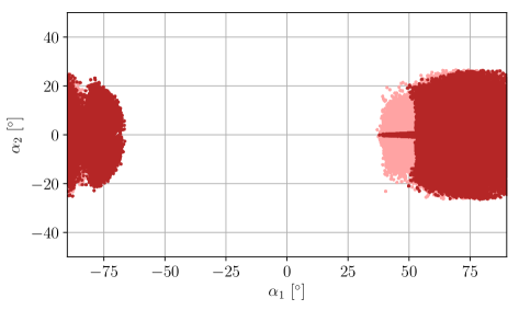
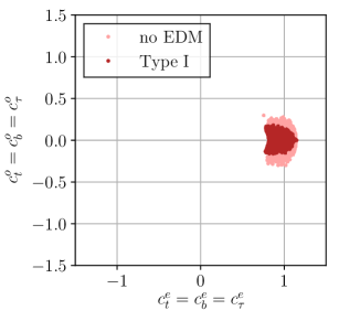
Figure 1: C2HDM Type I: For sample 1 (dark) and sample 2 (light) left: mixing angles $\alpha_{1}$ and $\alpha_{2}$ of the C2HDM mixing matrix $R$ only including scenarios where $H_{1}=h_{125}$; right: Yukawa couplings.

The left plot of figure 1 displays the mixing angles $\alpha_{1}$, which (in the displayed case of $H_{1}=h_{125}$) mixes the CP-even parts of the two Higgs doublets and $\alpha_{2}$, which parametrises the amount of CP-violating pseudoscalar admixture, for Type I. In the right plot we present the CP-odd and the CP-even components of the Yukawa couplings for the Type I model with and without the EDM constraints. Both plots clearly show that the EDM constraints have little effect on the mixing angle $|\alpha_{2}|$, which can go up to 25^∘ when all constraints are taken into account.

The maximum value of this angle can be understood from the bound $0.79<\mu_{VV}<1.48$. In fact, as previously shown in Fontes:2015mea the fact alone that $\mu_{VV}>0.79$ forces the angle $|\alpha_{2}|$ to be below $\approx 27^{o}$. Coming from the bound on $\mu_{VV}$, this constraint will be approximately the same for all types (before imposing EDM constraints), as will become clear in the next plots.

We are also interested in the wrong-sign regime, defined by a relative sign of the Yukawa coupling compared to the Higgs-gauge coupling, realized for $c_{b}^{e}<0$. As shown previously in Ferreira:2014naa ; Ferreira:2014dya , the right plot again demonstrates that the wrong-sign regime is in conflict with the Type I constraints because the Yukawa couplings cannot be varied independently.

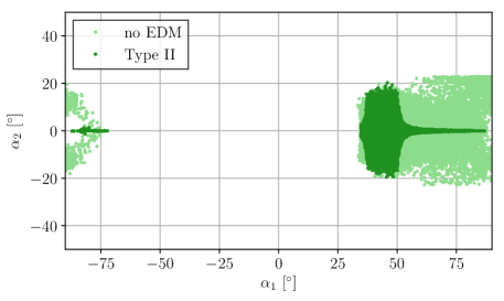
Figure 2: Type II, $H_{1}=h_{125}$: Mixing angles $\alpha_{1}$ and $\alpha_{2}$ of the C2HDM Type II mixing matrix $R$ for sample 1 (dark) and sample 2 (light).

In figure 2 we present the distributions of the angle $\alpha_{1}$ and $\alpha_{2}$ for samples 1 and 2 and for a Type II model. The EDM constraints, applied in our sample 1, strongly reduce $|\alpha_{2}|$ to small values. Only for scenarios around the maximal doublet mixing case with $\alpha_{1}\approx\pi/4$, $\alpha_{2}$ can reach values of up to $\sim\pm 20^{\circ}$.

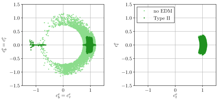
Figure 3: C2HDM Type II, $h_{125}=H_{1}$: Yukawa couplings to bottom quarks and tau leptons (left) and top quarks (right) for sample 1 (dark) and sample 2 (light).

The phenomenological implications of the reduced CP-violating mixing angle in Type II when $h_{125}=H_{1}$ are demonstrated in figure 3. It shows the distribution of the CP-odd component $c^{o}_{f}$ versus the CP-even component $c^{e}_{f}$ of the $h_{125}$ Yukawa coupling as defined in eq. (2.56) to bottom quarks and tau leptons (left) and top quarks (right). As can be inferred from figure 3 (left) the Higgs data alone still allow for vanishing scalar couplings to down-type quarks ($c^{e}_{b}=0$), as discussed in Fontes:2015mea . The inclusion of the EDM constraints, however, clearly rules out this possibility when $h_{125}=H_{1}$. Nevertheless, the wrong-sign regime ($c_{b}^{e}<0$) is still possible in the C2HDM for down-type Yukawa couplings. The electron EDM has no discernable effect on the allowed coupling to up-type quarks, as can be read off from the right plot.

The situation changes when we take Type II with $h_{125}=H_{2}$, as shown in figure 4.

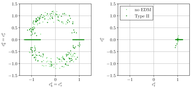
Figure 4: C2HDM Type II, $h_{125}=H_{2}$: Yukawa couplings to bottom quarks (left) and top quarks (right) for sample 1 (dark) and sample 2 (light).

One can still find scenarios where the top coupling is mostly CP-even ($c_{t}^{e}\simeq 1$), while the bottom coupling is mostly CP-odd ($c_{b}^{o}\simeq 1$). It is noteworthy that the electron EDM kills all such points in Type II when $h_{125}=H_{1}$, but that they are still allowed in Type II when $h_{125}=H_{2}$.

In table 3 we present three benchmark scenarios in Type II with large CP-violation in the Yukawa sector. The first scenario, BP2m, has maximal $c^{o}_{b}$ with nearly vanishing $c^{e}_{b}$. Since $c^{e}_{t}$ is always $\simeq 1$ this means that $c^{e}_{t}c^{o}_{b}$ is maximal here. The other two scenarios BP2c and BP2w both have maximal $c^{e}_{b}c^{o}_{b}$ but are in the correct sign and wrong-sign regime, respectively. As discussed above all of the scenarios with large CP-violation in the Yukawa couplings of $h_{125}$ require $H_{2}=h_{125}$ in Type II models.

Type II	BP2m	BP2c	BP2w
$m_{H_{1}}$	94.187	83.37	84.883
$m_{H_{2}}$	125.09	125.09	125.09
$m_{H^{\pm}}$	586.27	591.56	612.87
$\mathrm{Re}(m_{12}^{2})$	24017	7658	46784
$\alpha_{1}$	-0.1468	-0.14658	-0.089676
$\alpha_{2}$	-0.75242	-0.35712	-1.0694
$\alpha_{3}$	-0.2022	-0.10965	-0.21042
$\tan\beta$	7.1503	6.5517	6.88
$m_{H_{3}}$	592.81	604.05	649.7
$c^{e}_{b}=c^{e}_{\tau}$	0.0543	0.7113	-0.6594
$c^{o}_{b}=c^{o}_{\tau}$	1.0483	0.6717	0.6907
$\mu_{V}/\mu_{F}$	0.899	0.959	0.837
$\mu_{VV}$	0.976	1.056	1.122
$\mu_{\gamma\gamma}$	0.852	0.935	0.959
$\mu_{\tau\tau}$	1.108	1.013	1.084
$\mu_{bb}$	1.101	1.012	1.069

Table 3: Benchmark points with large pseudoscalar Yukawa couplings in Type II, $h_{125}=H_{2}$. Lines 1-8 contain the input parameters; lines 9-11 the derived third Higgs boson mass and the relevant Yukawa couplings (multiplied by $\mathrm{sgn}(c(h_{125}VV))$) and the last five lines the signal strengths of $h_{125}$.

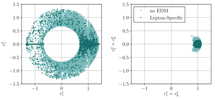
Figure 5: C2HDM Lepton-Specific: Yukawa couplings to charged leptons (left) and bottom and top quarks (right) for sample 1 (dark) and sample 2 (light).

The situation is even more interesting in the other two Yukawa types. Figure 5 displays the Yukawa couplings for the Lepton-Specific model with and without the EDM constraints. The down-type quark couplings are tied to the up-type couplings and, thus, heavily constrained to lie close to the SM (fully CP-even) solution. However, figure 5 (left) shows that the charged lepton couplings can still be mostly (or even fully) CP-odd, despite the current EDM constraints.

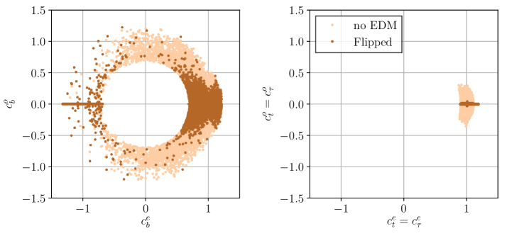
Figure 6: C2HDM Flipped: Yukawa couplings to bottom quarks (left) and charged leptons and top quarks (right) for sample 1 (dark) and sample 2 (light).

Similarly, in the Flipped model the bottom quark can couple to $h_{125}$ in a fully CP-odd fashion, as shown in the left plot of figure 6. In it, we display the Yukawa couplings for the Flipped model with and without the EDM constraints.

As will be discussed below, such large CP-odd components are still viable in both Lepton-Specific and Flipped models due to cancellations between the various diagrams entering the EDM calculation. This is also true for Type II when $H_{2}=h_{125}$. But it is important to stress that they are not due to large $\alpha_{2}$ values, as illustrated in figure 7.

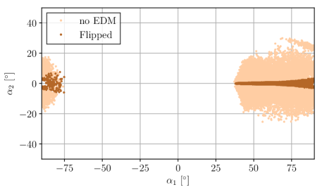
Figure 7: C2HDM Flipped: Mixing angles $\alpha_{1}$ and $\alpha_{2}$ of the mixing matrix $R$ for sample 1 (dark) and sample 2 (light).

The values for $\alpha_{2}$ are small, but $c^{o}(h_{125}b\bar{b})$ grows very fast as $\alpha_{2}$ departs from $\alpha_{2}=0$ for large $\tan{\beta}$. It grows roughly as $c^{o}(h_{125}b\bar{b})\sim s_{2}\tan{\beta}$.

LS	BPLSm	BPLSc	BPLSw		Flipped	BPFm	BPFc	BPFw
$m_{H_{1}}$	125.09	125.09	91.619		$m_{H_{1}}$	125.09	125.09	125.09
$m_{H_{2}}$	138.72	162.89	125.09		$m_{H_{2}}$	154.36	236.35	148.75
$m_{H^{\pm}}$	180.37	163.40	199.29		$m_{H^{\pm}}$	602.76	589.29	585.35
$\mathrm{Re}(m_{12}^{2})$	2638	2311	1651		$\mathrm{Re}(m_{12}^{2})$	10277	8153	42083
$\alpha_{1}$	-1.5665	1.5352	0.0110		$\alpha_{1}$	-1.5708	1.5277	-1.4772
$\alpha_{2}$	0.0652	-0.0380	0.7467		$\alpha_{2}$	-0.0495	-0.0498	0.0842
$\alpha_{3}$	-1.3476	1.2597	0.0893		$\alpha_{3}$	0.7753	0.4790	-1.3981
$\tan\beta$	15.275	17.836	9.870		$\tan\beta$	18.935	14.535	8.475
$m_{H_{3}}$	206.49	210.64	177.52		$m_{H_{3}}$	611.27	595.89	609.82
$c^{e}_{\tau}$	-0.0661	0.6346	-0.7093		$c^{e}_{b}$	-0.0003	0.6269	-0.7946
$c^{o}_{\tau}$	0.9946	0.6780	-0.6460		$c^{o}_{b}$	-0.9369	0.7239	0.7130
$\mu_{V}/\mu_{F}$	0.980	0.986	0.954		$\mu_{V}/\mu_{F}$	0.927	0.964	0.844
$\mu_{VV}$	1.014	1.029	1.000		$\mu_{VV}$	1.154	1.091	0.998
$\mu_{\gamma\gamma}$	0.945	1.018	0.879		$\mu_{\gamma\gamma}$	1.027	0.986	0.874
$\mu_{\tau\tau}$	1.007	0.880	0.943		$\mu_{\tau\tau}$	1.148	1.084	1.039
$\mu_{bb}$	1.013	1.020	1.025		$\mu_{bb}$	1.001	0.992	1.170

Table 4: Benchmark points with large pseudoscalar Yukawa couplings in the Lepton-Specific (LS) and Flipped types. Lines 1-8 contain the input parameters; lines 9-11 the derived third Higgs mass and the relevant Yukawa couplings (multiplied by $\mathrm{sgn}(c(h_{125}VV))$) and the last five lines the signal strengths of $h_{125}$.

In table 4 we present further benchmark scenarios in the Lepton-Specific and Flipped types. The BPLSm scenario has a maximal $c^{o}_{\tau}$ coupling with tiny $c^{e}_{\tau}$, thus here $h_{125}$ appears CP-even in its couplings to quarks and CP-odd in its couplings to leptons. In BPLSc and BPLSw the product $c^{e}_{\tau}c^{o}_{\tau}$ is maximal. In the Flipped model we provide three benchmark points. The first one, BPFm, again having maximal $c^{o}_{b}$ while BPFc and BPFw both have large $c^{o}_{b}c^{e}_{b}$ but with opposite signs and are therefore close to the correct and wrong-sign limit, respectively. Note that, in contrast to the Type II, all benchmark points except BPLSw have $H_{1}=h_{125}$. We chose BPLSw with $H_{2}=h_{125}$ since maximising $c^{e}_{\tau}c^{o}_{\tau}$ close to the wrong-sign limit of the Lepton-Specific model leads to this mass ordering.

3.3 The case $H_{3}=h_{125}$

One interesting possibility in the C2HDM is to have the 125 GeV scalar discovered at LHC ($h_{125}$) coincide with the heaviest Higgs boson ($H_{3}$). This possibility is excluded for Type II and Flipped, as the $B$-physics constraints impose that the charged Higgs boson must be quite heavy, $m_{H^{+}}>580$ GeV. This poses a problem with the electroweak precision tests, specially with the $T$ parameter. Indeed, the way to accommodate the experimental bounds on $T$ is to have a spectrum that has some degree of degeneracy. Requiring $m_{H^{+}}>580$ GeV implies that the other Higgs boson masses cannot all be below 125 GeV. Thus, $m_{H^{+}}>580$ GeV is not compatible with $m_{H_{2}}<125$ GeV.

However, $H_{3}=h_{125}$ is feasible for Type I and Lepton-Specific, as in these cases $B$-physics constraints only impose $m_{H^{+}}>100$ GeV (as explained, for low $\tan\beta$ this bound could be slightly higher). The situation here is quite fascinating, because it highlights an interesting complementarity between LHC and the old LEP results. The relevant Feynman rules are:

$$[H_{k}Z_{\mu}Z_{\nu}]:\ \ ig_{\mu\nu}\frac{g}{c_{W}}m_{Z}\,c(H_{k}ZZ),$$

$$[H_{i}H_{j}Z_{\mu}]:\ \ i\frac{g}{2c_{W}}(p_{i}-p_{j})_{\mu}\,c(H_{i}H_{j}Z),$$ (3.65)

where $p_{i}$ and $p_{j}$ are the incoming momenta of particles $H_{i}$ and $H_{j}$, respectively, $c(H_{k}ZZ)$ is given in eq. (2.55), and

$$c(H_{i}H_{j}Z)=\epsilon_{ijk}\,c(H_{k}ZZ).$$ (3.66)

In the SM, $c(H_{k}ZZ)=1$ and $c(H_{i}H_{j}Z)=0$. Equating $H_{3}=h_{125}$, the LHC $h_{125}\to ZZ$ signal forces $c(H_{3}ZZ)\sim 1$. But this means that $c(H_{1}H_{2}Z)\sim 1$ and, if $m_{H_{3}}>m_{H_{1}}+m_{H_{2}}$, then the decay $Z\to H_{1}H_{2}$ would have been seen at LEP Schael:2006cr . Thus, all points with $H_{3}=h_{125}$ must have $m_{H_{3}}<m_{H_{1}}+m_{H_{2}}\leq 2m_{H_{2}}$. If $m_{H_{3}}>2m_{H_{1}}$ the decay $H_{3}\to H_{1}H_{1}$ is possible. This decay is still possible in Type I and Lepton-Specific, as shown in figure 8. In fact, the rates can go up to about 10 pb and therefore have excellent prospects of being probed at the LHC Run2. If we include the decays of the $H_{1}$ we retain cross sections of up to 1 pb in the $H_{3}\to H_{1}H_{1}\to b\bar{b}\tau^{+}\tau^{-}$ channel in both models and up to 50 fb in the $H_{3}\to H_{1}H_{1}\to b\bar{b}\gamma\gamma$ channel in Type I.

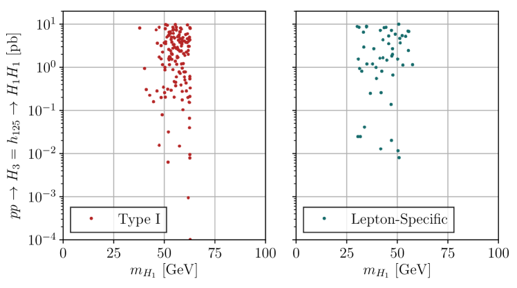
Figure 8: Rate for $pp\to H_{3}(=h_{125})\to H_{1}H_{1}$. There are only allowed points for Type I (left) and for Lepton-Specific (right).

Notably, even within this subset of points, one can still find Lepton-Specific corners of parameter space which obey EDM constraints and still allow for large CP-odd components in $c^{o}(h_{125}\tau\bar{\tau})$.

4 Measures of CP-violation

Throughout this section we will use the notation $H_{\downarrow}$ ($H_{\uparrow}$) to designate the lightest (heaviest) of the non-$h_{125}$ neutral Higgs bosons. Their mass can be below or above 125 GeV. The manifestation of CP-violation in models with two Higgs doublets can be probed with a number of variables even if there is only one independent CP-violating phase in the scalar sector. The most obvious variable is the phase in one of the complex parameters of the potential, that is, either $\lambda_{5}$ or $m_{12}^{2}$. As the two phases are not independent, we have opted to use $\phi(\lambda_{5})$. As discussed in Branco:1999fs ; Fontes:2015xva , there are several combinations of Higgs decays that are a clear signal of CP-violation in any extension of the SM. Others, like the simultaneous observation of the three decays $H_{i}\to ZZ$, $i=1,2,3$, enable us to distinguish the 2HDM from the C2HDM but are not unequivocal signs of CP-violation in general extensions of the SM. The question we are trying to address now is: are there variables that quantify CP-violation from a theoretical point of view and also correlate with the rates of a combination of decays which would establish CP-violation experimentally?

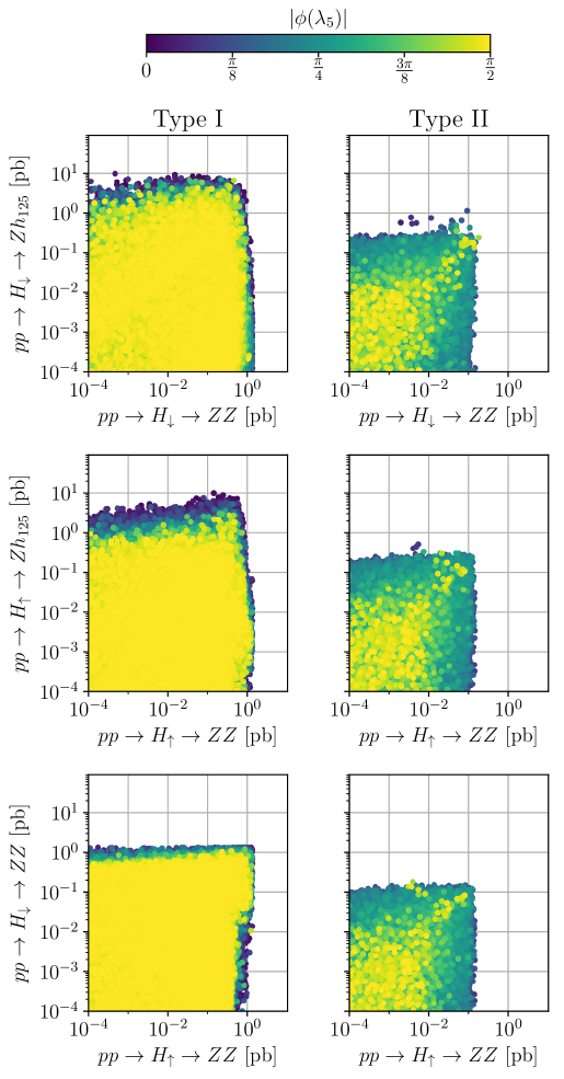
Figure 9: Set of CP-violating processes as a function of the CP-violation phase $|\phi(\lambda_{5})|$ (see colour code) for Type I (left column) and Type II (right column). In the first row we show $pp\to H_{\downarrow}\to Zh_{125}$ against $pp\to H_{\downarrow}\to ZZ$, in the second row we have $pp\to H_{\uparrow}\to Zh_{125}$ against $pp\to H_{\uparrow}\to ZZ$ and in the third row we plot $pp\to H_{\downarrow}\to ZZ$ against $pp\to H_{\uparrow}\to ZZ$. Note that the yellow points are superimposed on the darker points - there are dark points underneath the yellow points.

Starting with $\phi(\lambda_{5})$, we present in figure 9 three classes of CP-violating processes as a function of the CP-violation phase $|\phi(\lambda_{5})|$ for Type I (left column) and Type II (right column). In the first row we show $pp\to H_{\downarrow}\to Zh_{125}$ against $pp\to H_{\downarrow}\to ZZ$, in the second row we have $pp\to H_{\uparrow}\to Zh_{125}$ against $pp\to H_{\uparrow}\to ZZ$ and in the third row we plot $pp\to H_{\downarrow}\to ZZ$ against $pp\to H_{\uparrow}\to ZZ$. These classes of decays were chosen because together with the already observed process $h_{125}\to ZZ$ they can be used to identify CP violation, and also because searches for the other processes were performed for Run 1 and will continue during Run 2. There are two striking features in the plots. First, the production rates in Type I are almost one order of magnitude above the ones for Type II. This is because there are constraints that act more strongly on Type II like $b\to s\gamma$ or the EDM constraints as we will see later. Ultimately, it is due to the different structure of the Yukawa couplings: in Type I all Yukawa couplings are equal, making the model harder to constrain. Second, there is no correlation between the magnitude of $\phi(\lambda_{5})$ and the production rates, because the points with larger $\phi(\lambda_{5})$ are almost evenly spread throughout the plot. It is not that we expected that large values of the CP-violating phase would correspond to large production rates for any of the processes in the plot. In fact, maximal CP-violation is attained for specific sets of values of the angles but the production rates are a complicated combination of all parameters of the model. Still some colour structure could have emerged in the plots, but this was not the case.

In view of the negative result for the complex phase, we have looked for other variables Mendez:1991gp ; Khater:2003ym that could be used as a measure of CPV in the production and decay of the three neutral Higgs bosons Branco:1999fs ; Fontes:2015xva . The sets of variables proposed in the literature are basically of two types: the ones where the CP-violating variables appear in a sum of squares, and the ones where they appear in a product. The important difference between them is that while the former is zero only when there is no CP-violation in the model, the latter can be zero even if the model is CP-violating. However, if CP is conserved, both variables are zero.

We start by defining a multiplicative variable first proposed in Mendez:1991gp that allows us to distinguish a CP-conserving from a CP-violating 2HDM,

$$\xi_{V}=27[g_{h_{1}VV}\,g_{h_{2}VV}\,g_{h_{3}VV}]^{2}=27\prod_{i=1}^{3}[\cos\beta R_{i1}+\sin\beta R_{i2}]^{2}=27\prod_{i=1}^{3}T_{1i}^{2}\,,$$ (4.67)

which, when the couplings $g_{VVH_{i}}$ are normalised to the SM one, satisfies

$$0\leq\xi_{V}\leq 1.$$ (4.68)

With the purpose of finding quantities invariant under a basis transformation that change sign under a CP transformation, it was shown in Lavoura:1994fv that the simplest CP-odd invariant that can be built from the mass matrix is

$$J_{1}=(m_{1}^{2}-m_{2}^{2})(m_{1}^{2}-m_{3}^{2})(m_{2}^{2}-m_{3}^{2})\prod_{i=1}^{3}T_{1i}\,.$$ (4.69)

Furthermore, any other CP-odd invariant built from the mass matrix alone has to be proportional to $J_{1}$ Lavoura:1994fv . There is a relation between $\xi_{V}$ and $J_{1}^{2}$ that can be written as

$$J_{1}^{2}=[(m_{1}^{2}-m_{2}^{2})(m_{1}^{2}-m_{3}^{2})(m_{2}^{2}-m_{3}^{2})]^{2}\frac{\xi_{V}}{27}\,.$$ (4.70)

It should be noted that even if $J_{1}=0$, CP-violation could occur in the scalar sector (see Lavoura:1994fv for details).

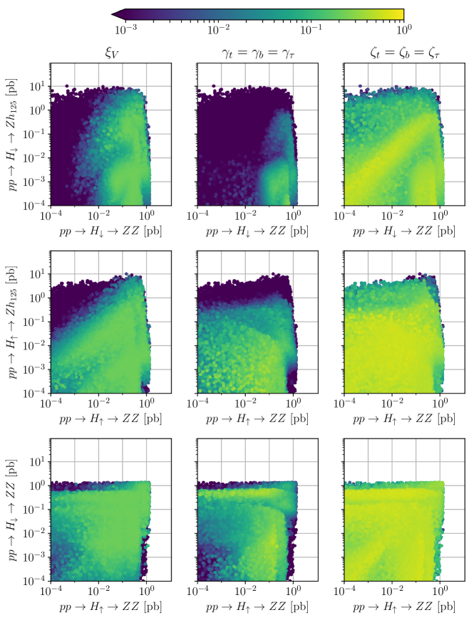
Figure 10: Classes of CP-violating processes as a function of the CP-violating variables (see colour code) for the Type I C2HDM. In the first row we show $pp\to H_{\downarrow}\to Zh_{125}$ against $pp\to H_{\downarrow}\to ZZ$, in the second row we have $pp\to H_{\uparrow}\to Zh_{125}$ against $pp\to H_{\uparrow}\to ZZ$ and in the third row we plot $pp\to H_{\downarrow}\to ZZ$ against $pp\to H_{\uparrow}\to ZZ$. In each column we show the variable that is being probed. The darker points are underneath the lighter ones.

This measure of CP-violation is not applicable to the fermion–Higgs sector, where the invariants of ref. Botella:1994cs apply instead. Variables that are a clear signal of CP-violation can be built with the scalar and pseudoscalar components of the Yukawa couplings. In fact, if a model has CP-violating scalars at tree level its Yukawa couplings have the general form $c^{e}_{f}+ic^{o}_{f}\gamma_{5}$. Thus, as discussed at the beginning of subsection 3.2, variables of the type $c^{e}c^{o}$ clearly signal CP-violation in the model. Therefore, we define the normalised multiplicative variables Khater:2003ym

$$\gamma_{t}=1024\prod_{i=1}^{3}[R_{i2}\,R_{i3}]^{2},\quad\gamma_{b}=1024\prod_{i=1}^{3}[R_{i1}\,R_{i3}]^{2},$$ (4.71)

satisfying

$$0\leq\gamma_{t}\leq 1,\quad 0\leq\gamma_{b}\leq 1,$$ (4.72)

as measures of CP-violation in the up- and down-quark sectors, respectively. The corresponding normalised sum variables Khater:2003ym are defined as

$$\zeta_{t}=2\sum_{i=1}^{3}[R_{i2}\,R_{i3}]^{2},\quad\zeta_{b}=2\sum_{i=1}^{3}[R_{i1}\,R_{i3}]^{2}\,,$$ (4.73)

with

$$\quad 0\leq\zeta_{t}\leq 1,\,\qquad 0\leq\zeta_{b}\leq 1,$$ (4.74)

again for the up- and down-quark sectors, respectively.

We will use the same combinations of decays as in figure 9 to see if any of the variables proposed can provide a relation between the amount of CP-violation and the production rates in case these processes are observed at the LHC. In figure 10 we present the three classes that signal CP-violation as a function of the CP-violation variables for the Type I C2HDM. Since $h_{125}\to ZZ$ (not shown) was already observed, any pair of two processes appearing in the plots combined with the latter form a signal of CP-violation. In the first row we show $pp\to H_{\downarrow}\to Zh_{125}$ against $pp\to H_{\downarrow}\to ZZ$, in the second row we have $pp\to H_{\uparrow}\to Zh_{125}$ against $pp\to H_{\uparrow}\to ZZ$ and in the third row we plot $pp\to H_{\downarrow}\to ZZ$ against $pp\to H_{\uparrow}\to ZZ$. In each column, we show the variable that is being probed. For the case of Type I, the top and bottom Yukawa couplings are the same. The general picture is that there is no striking correlation between the large values for the variables (more yellow points) and the large production cross sections for each process. There is a quite even spread of yellow points for the sum variable, $\zeta_{f}$. This is because even if the product of scalar/pseudoscalar components of the SM-like Higgs boson is very constrained, any of the products of the other two Higgs bosons can be very large, yielding a large value for the sum in $\zeta_{f}$. Therefore, variables of this type can always be large, and we will not show them in the remaining plots. Regarding the variables $\gamma_{f}$, we can see some structure in the plots as there are cases where more yellow points are clustered closer to the maximum values of the production rates. This trend is clearer in the last row where kinematics play a less important role. In fact, the first row is the most constrained regarding the phase space available while the last row is almost symmetric regarding the reduction of the phase space. The difference between the first and second row regarding kinematics is just that the first row deals with the lightest non-125 Higgs boson while the second row deals with the heaviest one.

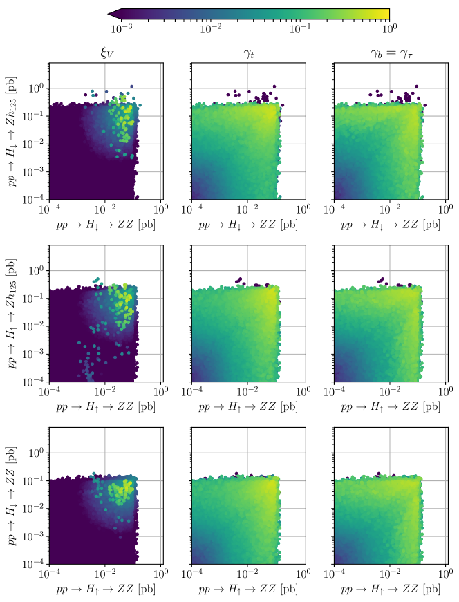
Figure 11: Same as figure 10, but for Type II.

In figure 11 we present the same three classes of CP-violating processes as a function of CP-violating variables for the Type II C2HDM. What we see for this Yukawa type is that the distribution of the yellow points is more structured and more clustered in specific regions. In fact, the yellow points tend to cluster more in the regions where the production rates are larger. This behaviour is more striking in the first column, for the variable $\xi_{V}$, where all yellow points are in the parameter region where the production rates are maximal. For the remaining variables, the distribution of yellow points is again not so structured. Still, all variables are larger when the production rates are both large and are much smaller when both production rates are smaller. However, in all plots, there are always points with small values of the CP-violating variables and large values of the production rates. Hence, although the variables show us a trend, they are not conclusive as a measure of CP-violation in the scalar sector.

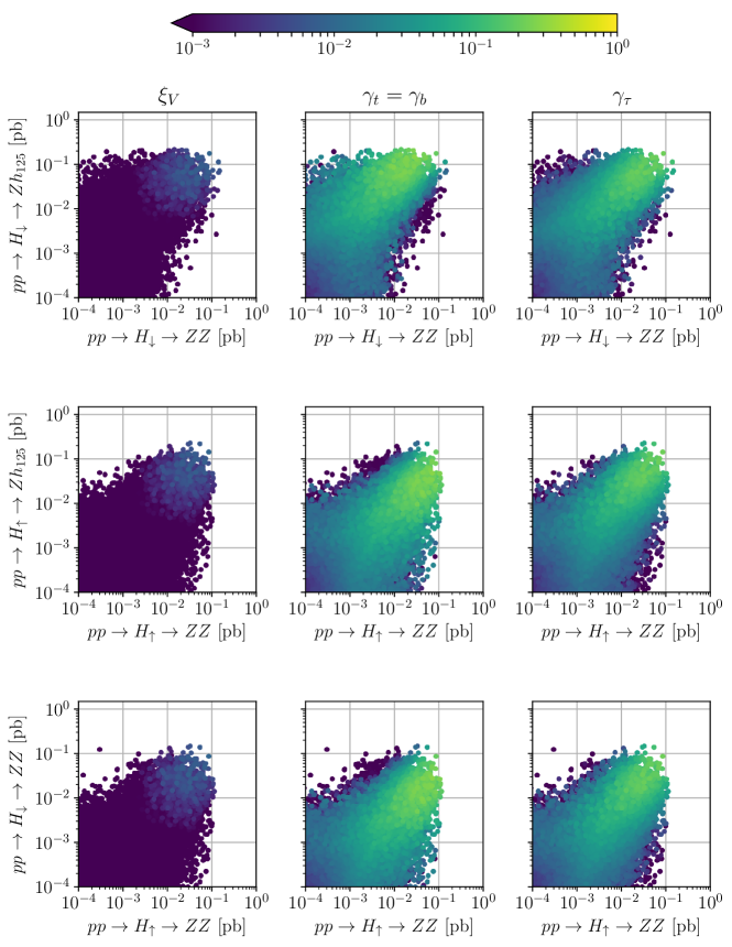
Figure 12: Same as figure 11, but with signal strengths within 5% of the SM values, for Type II.

In figure 12 we present the same classes in the Type II C2HDM as in figure 11, but with signal strengths (see eq. (3.60)) within 5% of the SM values. This gives us a hint on what to expect at the end of the LHC Run2, or at the high luminosity LHC. There is a clear effect in reducing the production rates but not in the distribution of yellow points. The main difference is that now no yellow points appear in the first column which means that the points with very large rates were excluded. The distribution of points in the other columns did not change significantly, but the points with the higher rates were also excluded as for the first row. In conclusion, there seems to be an overall reduction in the parameter space of the model leading to smaller production rates.

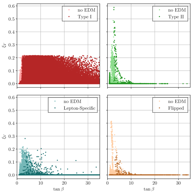
Figure 13: The CP-violating parameter $\xi_{V}$ as a function of $\tan\beta$ for Type I (top left), Type II (top right), Lepton-Specific (bottom left) and Flipped (bottom right). The lighter points have passed all the constraints except for the EDM bounds while the darker points have passed all constraints.

In figure 13 we show the CP-violating parameter $\xi_{V}$ as a function of $\tan\beta$ for Type I (top left), Type II (top right), Lepton-Specific (bottom left) and Flipped (bottom right). The lighter points have passed all the constraints except for the EDM bounds, while the darker points have passed all constraints. In Type I there is not much difference between the two sets of points, and there are no special regions regarding the allowed values of $\tan\beta$. Also, the maximum value for $\xi_{V}$ is around 0.2 almost independently of $\tan\beta$. For Type II, the results are much more striking. After imposing the EDM constraints, we end with two almost straight lines (one for $\tan\beta\approx 1$ and the other for $\xi_{V}\approx 0$), as well as a region around $\tan\beta\approx 3$ permitting values of $\xi_{V}$ up to 0.6. This means that $\tan\beta$ can only be large when we approach the CP-conserving limit except for a few points, which lie in the wrong-sign regime. Hence, in a Type II model, points with significant CP-violation can occur for $\tan\beta\approx 1$ in the alignment limit or for large $\tan\beta$ for the wrong sign limit. The situation in Flipped is similar to Type II, with a lower maximum value of $\xi_{V}\sim 0.2$ after imposing the EDM constraints.

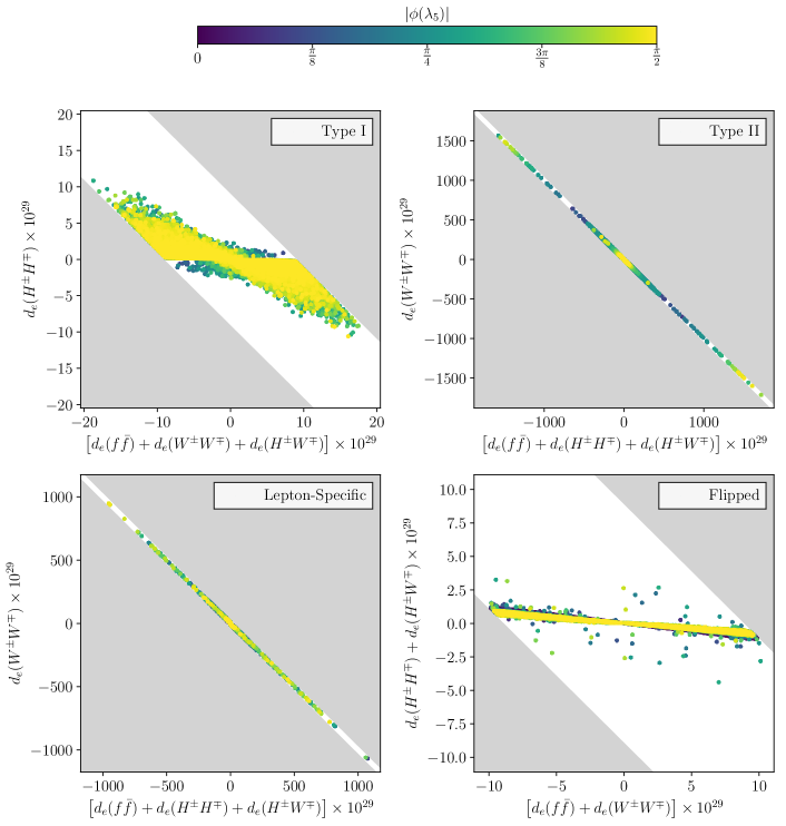
Figure 14: Contributions to the EDM according to their relative sign in Type I (top left), Type II (top right), Lepton-Specific (bottom left) and Flipped (bottom right). The colour code represents the absolute value of the magnitude of $\phi(\lambda_{5})$. The grey shaded regions represent the parameter space excluded by the EDM constraints only. The coloured points are the ones that passed all the constraints, that is, EDMs plus theoretical and all other experimental constraints.

In figure 14 we show the individual contributions to the EDM coming from $W$-loops, fermion-loops, charged Higgs loops and charged Higgs plus $W$-loops. For each C2HDM type, we have grouped the contributions to the EDM according to their relative sign. For example, in Type II the contributions of the $W$-loops (y-axis) and the sum of the contributions of the fermion loops, charged Higgs loops and charged Higgs plus $W$-loops (x-axis) have opposite sign. The grey shaded region represents the parameter space excluded by the EDM constraints only. The colour code represents the absolute value of the magnitude of $\phi(\lambda_{5})$. The first important difference between the models is that the maximum value of the individual contributions is around two orders of magnitude smaller in Type I than in Type II. This implies that Type I is less constrained by the EDM bounds. Therefore the remaining constraints play a much more important role in Type I than in Type II. This also leads to the distribution of values for the CP-violating phase in the figure. In Type II large values of $\phi(\lambda_{5})$ prefer regions where either the EDM contributions are very small, i.e. there are cancellations between loops in the individual contributions, or rely on huge cancellations between different contributions. This is in contrast to Type I, where large values of the CP-violating phase can be found all over the allowed region. The Flipped case behaves roughly like Type I, while the Lepton-Specific case behaves like Type II. This is very different from the usual behaviour of the Yukawa types. The reason is that most observables are dominated by quark effects giving similar behaviour to Type I/Lepton-Specific and Type II/Flipped. Since we are, however, looking at the EDM of the electron the lepton Yukawa couplings are the most important ones and those are equal in Type I/Flipped and Type II/Lepton-Specific.

Finally, it is important to comment on the different impact of the EDM constraints on the different models, regarding the possibility of having large pseudoscalar Yukawa couplings. For simplicity, we focus our discussion on the $H_{1}=h_{125}$ case. In Type I the pseudoscalar Yukawa couplings $c^{o}_{f}$ are proportional to $\sin(\alpha_{2})/\tan\beta$ for any fermion type $f$. Since $\alpha_{2}$ is at most of the order $20^{\circ}$ and $\tan\beta$ is constrained to be above 1, $c^{o}_{f}$ will be below about 0.4. For the other Yukawa types either $c^{o}_{b}$ or $c^{o}_{\tau}$ are proportional to $\sin(\alpha_{2})\tan\beta$. In this case, even if $\alpha_{2}$ is small the pseudoscalar coupling can be substantial for large $\tan\beta$. We have observed that in Type II the values of $\alpha_{2}$ can go up to $20^{\circ}$ while in the Flipped model they barely reach $5^{\circ}$. In both cases, $c_{b}^{o}$ could still be large because large values of $\tan\beta$ are allowed in both models. So what is the reason for having large $c^{o}_{b}$ for the Flipped model but not for Type II when $H_{1}=h_{125}$? The main reason is that the EDM constraints are less stringent in the Flipped model than in Type II due to relative signs between the CP-odd lepton Yukawa couplings and the remaining CP-odd Yukawa couplings. This ends up flipping several signs in one model relative to the other leading to cancellations between loops and much smaller individual EDM contributions. In Type II we found that this leads to the result that we can have large $\tan\beta$ only when $\alpha_{2}$ is very close to zero which is not the case for the Flipped model.

5 Higgs-to-Higgs decays

In the last section we have discussed the relation between some of the classes of decays that probe CP-violation with a number of variables proposed in the literature to measure CP-violation in the scalar sector. These particular classes were chosen not only because they can yield large production rates but also because there are currently searches being performed for these channels at the LHC that have already started during Run 1. There are, however, other classes of decays that can probe CP-violation and were the subject of a study that led to the production of benchmarks for Run 2 Fontes:2015xva ; deFlorian:2016spz . These other classes involve Higgs-to-Higgs decays such as $H_{i}\to h_{125}h_{125}$, $H_{j}\to H_{i}h_{125}$ and $h_{125}\to H_{i}H_{i}$. In this section we will study what is the role of the Higgs-to-Higgs decays in the search of CP-violation in the combination of three decays. The combination of the decays

$$H_{\downarrow\uparrow}\to h_{125}h_{125},\quad H_{\downarrow\uparrow}\to h_{125}Z,\quad h_{125}\to ZZ\,,$$ (5.75)

or also

$$h_{125}\to H_{\downarrow\uparrow}H_{\downarrow\uparrow},\quad h_{125}\to H_{\downarrow\uparrow}Z,\quad H_{\downarrow\uparrow}\to ZZ\,,$$ (5.76)

are a clear sign of CP-violation, and include Higgs-to-Higgs processes. Other classes like for instance

$$H_{\uparrow}\to h_{125}h_{125},\quad H_{\downarrow}\to h_{125}h_{125},\quad h_{125}\to ZZ\,.$$ (5.77)

are not possible in a CP-conserving 2HDM but are possible in the C2HDM. They are not, however, a sign of CP-violation. In fact, any model with three CP-even scalars can have this particular combination of three decays.

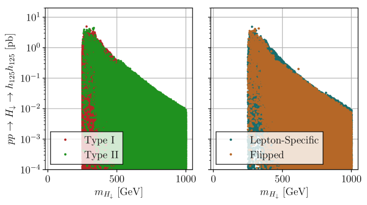
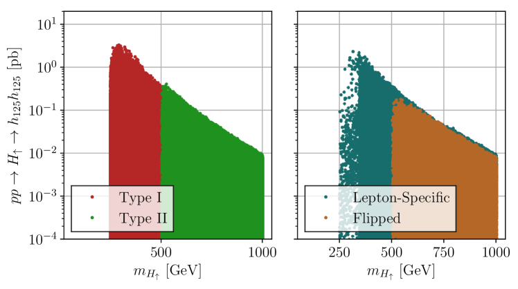
Figure 15: Production rates for the processes $pp\to H_{\downarrow}\to h_{125}h_{125}$ (top row) and $pp\to H_{\uparrow}\to h_{125}h_{125}$ (bottom row) as a function of the respective mass for all C2HDM types.

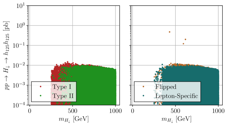
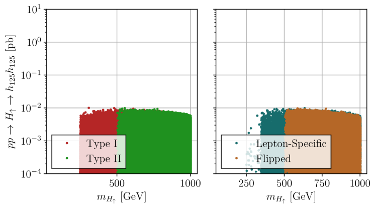
Figure 16: Production rates for the processes $pp\to H_{\downarrow}\to h_{125}h_{125}$ (top row) and $pp\to H_{\uparrow}\to h_{125}h_{125}$ (bottom row) as a function of the respective mass for the four C2HDM types (same as figure 15) but with the extra condition $\sigma(pp\to H_{\downarrow}\to ZZ)<1\,\textrm{fb}$ for the top plots and $\sigma(pp\to H_{\uparrow}\to ZZ)<1\,\textrm{fb}$ for the bottom plots.

In figure 15 we present the production rates for the processes $pp\to H_{\downarrow}\to h_{125}h_{125}$ (top row) and $pp\to H_{\uparrow}\to h_{125}h_{125}$ (bottom row) as a function of the respective mass for all C2HDM types. In all cases, the rates decrease as one increases the decaying scalar mass. In the four types, the $pp\to H_{\downarrow}\to h_{125}h_{125}$ rates can be quite large, reaching about 4 pb in all types. The maximum values are similar in Type I and Lepton-Specific for $pp\to H_{\uparrow}\to h_{125}h_{125}$. In contrast, for Type II and Flipped, the largest rates in $pp\to H_{\uparrow}\to h_{125}h_{125}$ decrease by about an order of magnitude because in these cases the heavier neutral scalar cannot be much lighter than the charged Higgs boson, which is heavy to comply with $B$-physics constraints. In order to understand how relevant the searches for the two scalar final states are we show in figure 16 the same rates as in the previous figure 15 but with the extra condition $\sigma(pp\to H_{\downarrow}\to ZZ)<1\,\textrm{fb}$ for the top plots and $\sigma(pp\to H_{\uparrow}\to ZZ)<1\,\textrm{fb}$ for the lower plots. It is clear from the plots that, with the extra restriction on the $ZZ$ final state, the cross sections now barely reach 10 fb for the two decay scenarios and for all types. Hence, although possible, it will be very hard to detect the new scalars in the $h_{125}h_{125}$ final state if they are not detected in the $ZZ$ final state. One should note that the cross section for di-Higgs production in the SM is about 33 fb. Consequently, a resonant di-Higgs final state such as the one presented in figure 15 would easily be detected because the cross sections can reach the pb level. However, it is also clear that once we force $\sigma(pp\to H_{\uparrow}\to ZZ)<1\,\textrm{fb}$ it is no longer possible to detect these di-Higgs states even at the High Luminosity LHC.

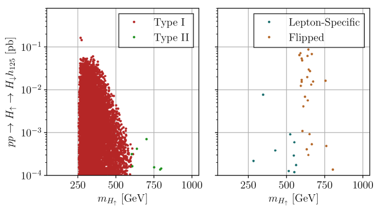
Figure 17: Production rates for the process $pp\to H_{\uparrow}\to H_{\downarrow}h_{125}$ as a function of the heavier Higgs boson mass, for all C2HDM types.

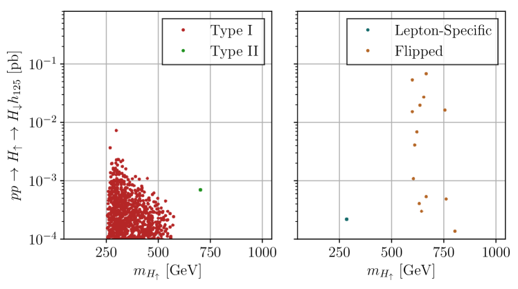
Figure 18: Production rates for the process $pp\to H_{\uparrow}\to H_{\downarrow}h_{125}$ as a function of the heavier Higgs boson mass, for all C2HDM types (same as figure 17) but with the extra condition $\sigma(pp\to H_{\uparrow}\to ZZ)<1\,\textrm{fb}$.

In figure 17 we show the production rates for the process $pp\to H_{\uparrow}\to H_{\downarrow}h_{125}$ as a function of the heavier Higgs mass, for all C2HDM types. For this channel the rates can reach at most about 100 fb, and only for Type I and Flipped. In Type II the rates are at most at the fb level. The rates for the $H_{\downarrow}h_{125}$ final state with the extra condition $\sigma(pp\to H_{\uparrow}\to ZZ)<1\,\textrm{fb}$ are shown in figure 18. The maximum rates (for low masses) are now reduced by about a factor of 5 for Type I. However, the rates do not decrease much for the Flipped C2HDM, and some signal at LHC Run 2 could point to this C2HDM type. Finally, although $H_{\uparrow}\to H_{\downarrow}h_{125}$ appears hard to detect in these models it is nevertheless a clear signal of non-minimal models and should therefore be a priority for the LHC Run 2.

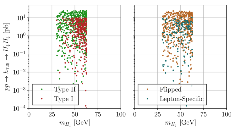
Figure 19: Production rates for the process $pp\to h_{125}\to H_{\downarrow}H_{\downarrow}$ as a function of the lighter Higgs boson mass.

We end this section with the production rate for the process $pp\to h_{125}\to H_{\downarrow}H_{\downarrow}$ as a function of the lighter Higgs mass for the various C2HDM types, which are shown in figure 19. Most points correspond to a mass of the heavier state above 125 GeV. But, as shown in figure 8, in the Type I and Lepton-Specific cases there are still solutions with $H_{3}=h_{125}$. Here the rates can be quite large if the lightest Higgs has a mass below 60 GeV. For this region the production rates can reach 10 pb (30 pb) for Type I and Lepton-Specific (for Type II and Flipped). In order to understand what would be the behaviour when choosing a definite final state, we have checked that the rates $pp\to h_{125}\to H_{\downarrow}H_{\downarrow}\to b\bar{b}\tau^{+}\tau^{-}$ are still above the pb level for all model types.

6 Conclusions

In this work we have analysed in detail a minimal complex version of the 2HDM, known as the C2HDM. The inclusion of all available experimental and theoretical constraints allowed us to present an up to date status of the model. We have shown that large CP-odd Yukawa couplings of $h_{125}$ are still possible in all Yukawa types except Type I. However, in Type II this is only a possibility if $H_{2}=h_{125}$. We provided two different interesting kinds of benchmark points which are in agreement with all current observations: for $h_{125}$ coupling like a scalar to some fermions and like a pseudoscalar to others, and for scenarios where the scalar and pseudoscalar Yukawa couplings of $h_{125}$ to some fermion are of similar size.

The model has only one CP-violating parameter. In previous works we have presented classes of three decays that are a clear sign of CP-violation, when all three are observed. In this work we looked for correlations between the production rates of the processes in each class and the phase $\phi(\lambda_{5})$ that measures CP-violation. We have shown that there is no correlation for the most relevant classes. We have then tested the correlation with other CP-violating variables proposed in the literature. The conclusion is that some correlation can be seen between the production rates and the variables. This is particularly true for the variable $\xi_{V}$ and even more for Type II. However, in most cases there is almost no correlation between the high rates of the CP-violating processes and the proposed CP-violating variables. The results also tell us that measuring small rates should not be interpreted as a sign of a small CP-violating angle.

Finally, we presented in the last section the production rates for the scenarios where the Higgs bosons decay to two other scalars. The search for a scalar decaying into two $h_{125}$ Higgs bosons was already performed during Run 1. However, the search for $H_{i}\to H_{j}h_{125}$ has not started yet. It is clear from the results that it will be much harder to probe CP-violation with classes of decays that involve scalar to scalar decays. However, on one hand it could be that all other decays would be very constrained. On the other hand, the observation of scalar to scalar decays would be a first step to reconstruct the Higgs potential. Hence, these searches should be a priority for Run 2 and especially for the high luminosity LHC.

As part of a common effort to a proper interpretation of the LHC results we release the code C2HDM_HDECAY that calculates the decay widths and branching ratios of all the C2HDM scalars including state-of-the-art QCD corrections.

Appendix

Appendix A Feynman rules for the C2HDM

We collect here the couplings of the neutral and charged Higgs bosons in the C2HDM in the unitary gauge. The conventions are that all particles and momenta are incoming into the vertex. As for the SM subset we use the notation for the covariant derivatives contained in Romao:2012pq , with all $\eta$’s positive. The complete set of Feynman rules for the C2HDM C2HDM_FR may be found at the url:

http://porthos.tecnico.ulisboa.pt/arXiv/C2HDM/

A.1 Couplings of neutral Higgs bosons to fermions

The couplings of neutral Higgs bosons to fermions can be written in general for all the neutral Higgs bosons of the model $H_{i}$ in a compact form

$$\mathcal{L}=-\frac{m_{f}}{v}\ \overline{f}\left[c^{e}(H_{i}ff)+i\gamma_{5}\,c^{o}(H_{i}ff)\right]f\,H_{i},$$ (A.1)

with the coefficients presented in table 2.

A.2 Couplings of charged Higgs bosons to fermions

The couplings of the charged Higgs bosons to fermions can be expressed in the following Lagrangian

$$\mathcal{L}=\frac{\sqrt{2}}{v}\,\overline{\psi}_{d_{i}}\left[\vbox to12.0pt{}m_{\psi_{d_{i}}}\eta_{L}P_{L}+m_{\psi_{u_{i}}}\eta_{R}P_{R}\right]\psi_{u_{i}}H^{-}+\frac{\sqrt{2}}{v}\,\overline{\psi}_{u_{i}}\left[\vbox to12.0pt{}m_{\psi_{d_{i}}}\eta_{L}P_{R}+m_{\psi_{u_{i}}}\eta_{R}P_{L}\right]\psi_{d_{i}}H^{+},$$ (A.2)

where $i$ are generation indices, $(\psi_{u_{i}},\psi_{u_{i}})=(u_{i},d_{i}),(\nu_{i},\ell_{i})$, for quarks and leptons in an obvious notation and $P_{L}=(1-\gamma_{5})/2$ and $P_{R}=(1+\gamma_{5})/2$. The couplings $\eta_{L,R}$ are given in table 5. In these expressions, we neglect the masses of the neutrinos, so in the last line in table 5 the zeros mean that the corresponding mass in eq. (A.2) is zero.

	Type I	Type II	Lepton	Flipped
			Specific
$\eta^{q}_{L}$	$-\cot\beta$	$\tan\beta$	$-\cot\beta$	$\tan\beta$
$\eta^{q}_{R}$	$\cot\beta$	$\cot\beta$	$\cot\beta$	$\cot\beta$
$\eta^{\ell}_{L}$	$-\cot\beta$	$\tan\beta$	$\tan\beta$	$-\cot\beta$
$\eta^{\ell}_{R}$	0	0	0	0

Table 5: Couplings of the charged Higgs bosons to fermions.

A.3 Cubic interactions of neutral Higgs bosons

The cubic interactions of neutral Higgs bosons, $[H_{i},H_{j},H_{k}]$, have long expressions. We do not write them here but we collect them in one web page C2HDM_FR . The expressions there are the Feynman rules without the $i$.

A.4 Cubic interactions of neutral and charged Higgs bosons

These are (on the right-hand side of these expressions we write the Feynman rule including the $i$),

$$[H_{i},H^{+},H^{-}] =-i\,v\left[\text{Im}(\lambda_{5})R_{i3}\cos(\beta)\sin(\beta)\right.$$

$$\hskip 42.67912pt+R_{i1}\cos(\beta)(\lambda_{3}\cos(\beta)^{2}-(\text{Re}(\lambda_{5})-\lambda_{1}+\lambda_{4})\sin(\beta)^{2})$$

$$\hskip 42.67912pt\left.+R_{i2}(-(\text{Re}(\lambda_{5})-\lambda_{2}+\lambda_{4})\cos(\beta)^{2}\sin(\beta)+\lambda_{3}\sin(\beta)^{3})\right]$$

$$\equiv i\,\lambda_{i}\,v\equiv i\,g_{H_{i}H^{+}H^{-}}\,,$$ (A.3)

where the $\lambda_{i}$ or $g_{H_{i}H^{+}H^{-}}$can be read from eq. (A.4). The $\lambda_{i}$ are in the notation used in ref. Fontes:2014xva and should not be confused with the parameters in the potential.

A.5 Cubic interactions with gauge bosons

One gauge boson

$$[H_{i},H^{\mp},W^{\pm\,\mu}] =\pm i\,\frac{g}{2}\left(p_{1}-p_{\mp}\right)^{\mu}\left(R_{i1}\sin(\beta)-R_{i2}\cos(\beta)\mp i\,R_{i3}\right)\,,$$ (A.4)

$$[H_{i},H_{j},Z^{\mu}] =\frac{g}{2c_{W}}\left(p_{i}-p_{j}\right)^{\mu}\epsilon_{ijk}\left[\cos(\beta)R_{k1}+\sin(\beta)R_{k2}\right]\,,$$ (A.5)

$$[A^{\mu},H^{+},H^{-}] =-i\;e\left(p_{+}-p_{-}\right)^{\mu}\,,$$ (A.6)

$$[H^{+},H^{-},Z^{\mu}] =-i\;\frac{g}{2c_{W}}(c_{W}^{2}-s_{W}^{2})\left(p_{+}-p_{-}\right)^{\mu}\,.$$ (A.7)

Two gauge bosons

$$[H_{i},W^{+}_{\mu},W^{-}_{\nu}] =i\,gM_{W}\,g_{\mu\nu}\left[R_{i1}\cos(\beta)+R_{i2}\sin(\beta)\right]\equiv i\,gM_{W}\,g_{\mu\nu}\ C_{i}\,,$$ (A.8)

$$[H_{i},Z_{\mu},Z_{\nu}] =i\,\frac{gM_{Z}}{c_{W}}\,g_{\mu\nu}\left[R_{i1}\cos(\beta)+R_{i2}\sin(\beta)\right]\equiv i\,\frac{gM_{Z}}{c_{W}}\,g_{\mu\nu}\ C_{i}\,,$$ (A.9)

where in eq. (A.8) and eq. (A.9) we used a notation to make contact with our previous conventions Fontes:2014xva .

A.6 Quartic interactions with Higgs bosons

Again these interactions involve quite long expressions and they are given in our web page C2HDM_FR . These include, $[H_{i},H_{j},H_{k},H_{l}]$ where $i,j,k,l=1,2,3$ and $[H_{i},H_{j},H^{-},H^{+}]$.

A.7 Quartic interactions with Gauge bosons

$$[A_{\mu},A_{\nu},H^{+},H^{-}] =2\,i\,e^{2}\,g_{\mu\nu}\,,$$ (A.10)

$$[A_{\mu},H_{i},H^{\mp},W^{\pm}_{\nu}] =-i\,\frac{eg}{2}\left[R_{i1}\sin(\beta)-R_{i2}\cos(\beta)\mp i\,R_{i3}\right]\,g_{\mu\nu}\,,$$ (A.11)

$$[H^{+},H^{-},W^{+}_{\mu},W^{-}_{\nu}] =i\,\frac{g^{2}}{2}\,g_{\mu\nu}\,,$$ (A.12)

$$[H_{i},H_{j},W^{+}_{\mu},W^{-}_{\nu}] =i\,\frac{g^{2}}{2}\,g_{\mu\nu}\,\delta_{ij}\,,$$ (A.13)

$$[A_{\mu},H^{+},H^{-},Z_{\nu}] =i\,\frac{eg}{c_{W}}(c_{W}^{2}-s_{W}^{2})g_{\mu\nu}\,,$$ (A.14)

$$[H_{i},H^{\mp},W^{\pm}_{\mu},Z_{\nu}] =i\,\frac{e^{2}}{2c_{W}}\left[R_{i1}\sin(\beta)-R_{i2}\cos(\beta)\mp i\,R_{i3}\right]\,g_{\mu\nu}\,,$$ (A.15)

$$[H^{+},H^{-},Z_{\mu},Z_{\nu}] =i\,\frac{g^{2}}{2c_{W}^{2}}(c_{W}^{2}-s_{W}^{2})^{2}g_{\mu\nu}\,,$$ (A.16)

$$[H_{i},H_{j},Z_{\mu},Z_{\nu}] =i\,\frac{g^{2}}{2c_{W}^{2}}g_{\mu\nu}\,\delta_{ij}\,.$$ (A.17)

Appendix B The Fortran Code C2HDM_HDECAY

The code C2HDM_HDECAY is the implementation of the CP-violating 2HDM in the program HDECAY v6.51 Djouadi:1997yw ; Butterworth:2010ym , which is written in Fortran77. All changes with respect to the C2HDM have been included in the main file hdecay.f, which is now called chdecay.f. Further linked routines have been taken over from the original HDECAY program, so that the code is completely self-contained. The decay widths are computed including the most important state-of-the-art higher order QCD corrections and the relevant off-shell decays. Note, that it does not include off-shell Higgs-to-Higgs decays, but only on-shell decays into a lighter Higgs pair. The QCD corrections can be taken over from the SM and the minimal supersymmetric extension (MSSM), respectively, for which HDECAY was originally designed. The electroweak corrections on the other hand cannot be adapted from the available corrections in the SM and/or MSSM so that they have been consistently turned off.

The C2HDM input parameters are specified in the input file c2hdecay.in which has been obtained by extending the original HDECAY input file hdecay.in. The C2HDM branching ratios and total widths are calculated after setting the input value C2HDM$=1$ in c2hdecay.in. The required input parameters are set in the block ’complex 2 Higgs Doublet Model’. Here the user specifies the values of two of the neutral Higgs boson masses, the third one is computed from the input values, and the charged Higgs boson mass. Furthermore, the mixing angles $\alpha_{1,2,3}$ and $\tan\beta$ have to be set as well as the real part of the mass parameter $M_{12}^{2}$. The type of the fermion sector is chosen via the input variable TYPE_cp. The values 1, 2, 3 and 4 correspond to the I, II, Lepton-Specific and Flipped types, respectively. For illustration, we display part of an example input file for the C2HDM case.

C2HDM    = 1...*********************** complex 2 Higgs Doublet Model *********************M1_2HDM  = 125.D0M2_2HDM  = 4.96226790D2MCH_2HDM = 4.9242445D2alp1_2HDM= 0.88941955D0alp2_2HDM= -0.096916989D0alp3_2HDM= 1.05235430D0tbetc2HDM= 1.19671762D0R_M12_H2 = 1.51744100D3TYPE_cp  = 2**************************************************************************...

The code is compiled with the file makefile. By typing make an executable file called run is produced. The program is executed with the command run. It calculates the branching ratios and total widths which are written out together with the mass of the decaying Higgs boson. The names of the output files are br.Xy_C2HDM. Here X=H1, H2, H3, c denotes the decaying Higgs particle, where ’$c$’ refers to the charged Higgs boson. Files with the suffix y=a contain the branching ratios into fermions, with y=b the ones into gauge bosons and the ones with y=c, d the branching ratios into lighter Higgs pairs or a Higgs-gauge boson final state. For illustration, we present the example of an output that has been obtained from the above input file. The produced output in the four output files br.H3y_C2HDM for the heaviest neutral Higgs boson is given by

   MH3         BB       TAU TAU     MU MU         SS         CC         TT
_______________________________________________________________________________

 506.461     0.1122E-02 0.1600E-03 0.5658E-06 0.4094E-06 0.2180E-04 0.9505
   MH3           GG     GAM GAM     Z GAM         WW         ZZ
_______________________________________________________________________________

 506.461     0.3149E-02 0.1046E-04 0.3603E-05 0.1324E-01 0.6341E-02
     MH3       Z H1       Z H2     W+- H-+
_______________________________________________________________________________

 506.461     0.1807E-01 0.5732E-08 0.1366E-06
      MH3      H1H1       H1H2       H2H2      H+ H-      WIDTH
_______________________________________________________________________________

 506.461     0.7417E-02  0.000      0.000      0.000      10.21

The program files can be downloaded at the url:

http://www.itp.kit.edu/$\sim$maggie/C2HDM

There one can find a short explanation of the program and information on updates and modifications of the program. Furthermore, sample output files are given for a sample input file.

References

- (1) ATLAS Collaboration collaboration, G. Aad et al., Observation of a new particle in the search for the Standard Model Higgs boson with the ATLAS detector at the LHC, Phys.Lett. B716 (2012) 1–29, [1207.7214].
- (2) CMS Collaboration collaboration, S. Chatrchyan et al., Observation of a new boson at a mass of 125 GeV with the CMS experiment at the LHC, Phys.Lett. B716 (2012) 30–61, [1207.7235].
- (3) A. D. Sakharov, Violation of CP Invariance, c Asymmetry, and Baryon Asymmetry of the Universe, Pisma Zh. Eksp. Teor. Fiz. 5 (1967) 32–35.
- (4) T. D. Lee, A Theory of Spontaneous T Violation, Phys. Rev. D8 (1973) 1226–1239.
- (5) J. F. Gunion, H. E. Haber, G. L. Kane and S. Dawson, The Higgs Hunter’s Guide, Front. Phys. 80 (2000) 1–404.
- (6) G. C. Branco, P. M. Ferreira, L. Lavoura, M. N. Rebelo, M. Sher and J. P. Silva, Theory and phenomenology of two-Higgs-doublet models, Phys. Rept. 516 (2012) 1–102, [1106.0034].
- (7) I. P. Ivanov, Building and testing models with extended Higgs sectors, Prog. Part. Nucl. Phys. 95 (2017) 160–208, [1702.03776].
- (8) I. F. Ginzburg, M. Krawczyk and P. Osland, Two Higgs doublet models with CP violation, in Linear colliders. Proceedings, International Workshop on physics and experiments with future electron-positron linear colliders, LCWS 2002, Seogwipo, Jeju Island, Korea, August 26-30, 2002, pp. 703–706, 2002, hep-ph/0211371, http://weblib.cern.ch/abstract?CERN-TH-2002-330.
- (9) W. Khater and P. Osland, CP violation in top quark production at the LHC and two Higgs doublet models, Nucl. Phys. B661 (2003) 209–234, [hep-ph/0302004].
- (10) A. W. El Kaffas, P. Osland and O. M. Ogreid, CP violation, stability and unitarity of the two Higgs doublet model, Nonlin. Phenom. Complex Syst. 10 (2007) 347–357, [hep-ph/0702097].
- (11) B. Grzadkowski and P. Osland, Tempered Two-Higgs-Doublet Model, Phys. Rev. D82 (2010) 125026, [0910.4068].
- (12) A. Arhrib, E. Christova, H. Eberl and E. Ginina, CP violation in charged Higgs production and decays in the Complex Two Higgs Doublet Model, JHEP 04 (2011) 089, [1011.6560].
- (13) A. Barroso, P. M. Ferreira, R. Santos and J. P. Silva, Probing the scalar-pseudoscalar mixing in the 125 GeV Higgs particle with current data, Phys. Rev. D86 (2012) 015022, [1205.4247].
- (14) S. Inoue, M. J. Ramsey-Musolf and Y. Zhang, CP-violating phenomenology of flavor conserving two Higgs doublet models, Phys. Rev. D89 (2014) 115023, [1403.4257].
- (15) K. Cheung, J. S. Lee, E. Senaha and P.-Y. Tseng, Confronting Higgcision with Electric Dipole Moments, JHEP 06 (2014) 149, [1403.4775].
- (16) D. Fontes, J. C. Romão and J. P. Silva, in the complex two Higgs doublet model, JHEP 12 (2014) 043, [1408.2534].
- (17) D. Fontes, J. C. Romão, R. Santos and J. P. Silva, Large pseudoscalar Yukawa couplings in the complex 2HDM, JHEP 06 (2015) 060, [1502.01720].
- (18) C.-Y. Chen, S. Dawson and Y. Zhang, Complementarity of LHC and EDMs for Exploring Higgs CP Violation, JHEP 06 (2015) 056, [1503.01114].
- (19) M. Muhlleitner, M. O. P. Sampaio, R. Santos and J. Wittbrodt, Phenomenological Comparison of Models with Extended Higgs Sectors, 1703.07750.
- (20) R. Grober, M. Muhlleitner and M. Spira, Higgs Pair Production at NLO QCD for CP-violating Higgs Sectors, 1705.05314.
- (21) J. F. Gunion and X.-G. He, Determining the CP nature of a neutral Higgs boson at the LHC, Phys. Rev. Lett. 76 (1996) 4468–4471, [hep-ph/9602226].
- (22) F. Boudjema, R. M. Godbole, D. Guadagnoli and K. A. Mohan, Lab-frame observables for probing the top-Higgs interaction, Phys. Rev. D92 (2015) 015019, [1501.03157].
- (23) S. Amor Dos Santos et al., Probing the CP nature of the Higgs coupling in events at the LHC, 1704.03565.
- (24) S. Berge, W. Bernreuther and J. Ziethe, Determining the CP parity of Higgs bosons at the LHC in their tau decay channels, Phys. Rev. Lett. 100 (2008) 171605, [0801.2297].
- (25) S. Berge and W. Bernreuther, Determining the CP parity of Higgs bosons at the LHC in the tau to 1-prong decay channels, Phys. Lett. B671 (2009) 470–476, [0812.1910].
- (26) S. Berge, W. Bernreuther, B. Niepelt and H. Spiesberger, How to pin down the CP quantum numbers of a Higgs boson in its tau decays at the LHC, Phys. Rev. D84 (2011) 116003, [1108.0670].
- (27) S. Berge, W. Bernreuther and S. Kirchner, Determination of the Higgs CP-mixing angle in the tau decay channels at the LHC including the Drell–Yan background, Eur. Phys. J. C74 (2014) 3164, [1408.0798].
- (28) S. Berge, W. Bernreuther and S. Kirchner, Prospects of constraining the Higgs boson’s CP nature in the tau decay channel at the LHC, Phys. Rev. D92 (2015) 096012, [1510.03850].
- (29) S. Y. Choi, D. J. Miller, M. M. Muhlleitner and P. M. Zerwas, Identifying the Higgs spin and parity in decays to Z pairs, Phys. Lett. B553 (2003) 61–71, [hep-ph/0210077].
- (30) C. P. Buszello, I. Fleck, P. Marquard and J. J. van der Bij, Prospective analysis of spin- and CP-sensitive variables in H —> Z Z —> l(1)+ l(1)- l(2)+ l(2)- at the LHC, Eur. Phys. J. C32 (2004) 209–219, [hep-ph/0212396].
- (31) R. M. Godbole, D. J. Miller and M. M. Muhlleitner, Aspects of CP violation in the H ZZ coupling at the LHC, JHEP 12 (2007) 031, [0708.0458].
- (32) ATLAS collaboration, G. Aad et al., Study of the spin and parity of the Higgs boson in diboson decays with the ATLAS detector, Eur. Phys. J. C75 (2015) 476, [1506.05669].
- (33) CMS collaboration, V. Khachatryan et al., Combined search for anomalous pseudoscalar HVV couplings in VH(H ) production and H VV decay, Phys. Lett. B759 (2016) 672–696, [1602.04305].
- (34) G. C. Branco, L. Lavoura and J. P. Silva, CP Violation, Int. Ser. Monogr. Phys. 103 (1999) 1–536.
- (35) D. Fontes, J. C. Romão, R. Santos and J. P. Silva, Undoubtable signs of -violation in Higgs boson decays at the LHC run 2, Phys. Rev. D92 (2015) 055014, [1506.06755].
- (36) A. Arhrib and R. Benbrik, Searching for a CP-odd Higgs via a pair of gauge bosons at the LHC, hep-ph/0610184.
- (37) W. Bernreuther, P. Gonzalez and M. Wiebusch, Pseudoscalar Higgs Bosons at the LHC: Production and Decays into Electroweak Gauge Bosons Revisited, Eur. Phys. J. C69 (2010) 31–43, [1003.5585].
- (38) L. Lavoura and J. P. Silva, Fundamental CP violating quantities in a SU(2) x U(1) model with many Higgs doublets, Phys. Rev. D50 (1994) 4619–4624, [hep-ph/9404276].
- (39) F. J. Botella and J. P. Silva, Jarlskog - like invariants for theories with scalars and fermions, Phys. Rev. D51 (1995) 3870–3875, [hep-ph/9411288].
- (40) A. Djouadi, J. Kalinowski and M. Spira, HDECAY: A Program for Higgs boson decays in the standard model and its supersymmetric extension, Comput. Phys. Commun. 108 (1998) 56–74, [hep-ph/9704448].
- (41) J. M. Butterworth et al., THE TOOLS AND MONTE CARLO WORKING GROUP Summary Report from the Les Houches 2009 Workshop on TeV Colliders, in Physics at TeV colliders. Proceedings, 6th Workshop, dedicated to Thomas Binoth, Les Houches, France, June 8-26, 2009, 2010, 1003.1643, http://inspirehep.net/record/848006/files/arXiv:1003.1643.pdf.
- (42) D. Fontes, M. Muhlleitner, J. C. Romão, R. Santos, J. P. Silva and J. Wittbrodt, Couplings of the C2HDM: http://porthos.tecnico.ulisboa.pt/arXiv/C2HDM/, October, 2017.
- (43) S. L. Glashow and S. Weinberg, Natural Conservation Laws for Neutral Currents, Phys. Rev. D15 (1977) 1958.
- (44) E. A. Paschos, Diagonal Neutral Currents, Phys. Rev. D15 (1977) 1966.
- (45) R. Coimbra, M. O. P. Sampaio and R. Santos, ScannerS: Constraining the phase diagram of a complex scalar singlet at the LHC, Eur. Phys. J. C73 (2013) 2428, [1301.2599].
- (46) R. Costa, M. Muhlleitner, M. O. P. Sampaio, R. Santos and J. Wittbrodt, ScannerS project, http://scanners.hepforge.org, October, 2016.
- (47) S. Kanemura, T. Kubota and E. Takasugi, Lee-Quigg-Thacker bounds for Higgs boson masses in a two doublet model, Phys. Lett. B313 (1993) 155–160, [hep-ph/9303263].
- (48) A. G. Akeroyd, A. Arhrib and E.-M. Naimi, Note on tree level unitarity in the general two Higgs doublet model, Phys. Lett. B490 (2000) 119–124, [hep-ph/0006035].
- (49) I. F. Ginzburg and I. P. Ivanov, Tree level unitarity constraints in the 2HDM with CP violation, hep-ph/0312374.
- (50) I. P. Ivanov and J. P. Silva, Tree-level metastability bounds for the most general two Higgs doublet model, Phys. Rev. D92 (2015) 055017, [1507.05100].
- (51) Gfitter Group collaboration, M. Baak, J. Cuth, J. Haller, A. Hoecker, R. Kogler, K. Monig et al., The global electroweak fit at NNLO and prospects for the LHC and ILC, Eur. Phys. J. C74 (2014) 3046, [1407.3792].
- (52) O. Deschamps, S. Descotes-Genon, S. Monteil, V. Niess, S. T’Jampens and V. Tisserand, The Two Higgs Doublet of Type II facing flavour physics data, Phys. Rev. D82 (2010) 073012, [0907.5135].
- (53) F. Mahmoudi and O. Stal, Flavor constraints on the two-Higgs-doublet model with general Yukawa couplings, Phys. Rev. D81 (2010) 035016, [0907.1791].
- (54) T. Hermann, M. Misiak and M. Steinhauser, in the Two Higgs Doublet Model up to Next-to-Next-to-Leading Order in QCD, JHEP 11 (2012) 036, [1208.2788].
- (55) M. Misiak et al., Updated NNLO QCD predictions for the weak radiative B-meson decays, Phys. Rev. Lett. 114 (2015) 221801, [1503.01789].
- (56) M. Misiak and M. Steinhauser, Weak Radiative Decays of the B Meson and Bounds on in the Two-Higgs-Doublet Model, Eur. Phys. J. C77 (2017) 201, [1702.04571].
- (57) LEP, DELPHI, OPAL, ALEPH, L3 collaboration, G. Abbiendi et al., Search for Charged Higgs bosons: Combined Results Using LEP Data, Eur. Phys. J. C73 (2013) 2463, [1301.6065].
- (58) H. E. Haber and H. E. Logan, Radiative corrections to the Z b anti-b vertex and constraints on extended Higgs sectors, Phys. Rev. D62 (2000) 015011, [hep-ph/9909335].
- (59) ATLAS, CMS collaboration, G. Aad et al., Combined Measurement of the Higgs Boson Mass in Collisions at and 8 TeV with the ATLAS and CMS Experiments, Phys. Rev. Lett. 114 (2015) 191803, [1503.07589].
- (60) P. Bechtle, O. Brein, S. Heinemeyer, G. Weiglein and K. E. Williams, HiggsBounds: Confronting Arbitrary Higgs Sectors with Exclusion Bounds from LEP and the Tevatron, Comput. Phys. Commun. 181 (2010) 138–167, [0811.4169].
- (61) P. Bechtle, O. Brein, S. Heinemeyer, G. Weiglein and K. E. Williams, HiggsBounds 2.0.0: Confronting Neutral and Charged Higgs Sector Predictions with Exclusion Bounds from LEP and the Tevatron, Comput. Phys. Commun. 182 (2011) 2605–2631, [1102.1898].
- (62) P. Bechtle, O. Brein, S. Heinemeyer, O. Stal, T. Stefaniak, G. Weiglein et al., : Improved Tests of Extended Higgs Sectors against Exclusion Bounds from LEP, the Tevatron and the LHC, Eur. Phys. J. C74 (2014) 2693, [1311.0055].
- (63) ATLAS, CMS collaboration, G. Aad et al., Measurements of the Higgs boson production and decay rates and constraints on its couplings from a combined ATLAS and CMS analysis of the LHC pp collision data at and 8 TeV, JHEP 08 (2016) 045, [1606.02266].
- (64) R. V. Harlander, S. Liebler and H. Mantler, SusHi: A program for the calculation of Higgs production in gluon fusion and bottom-quark annihilation in the Standard Model and the MSSM, Comput. Phys. Commun. 184 (2013) 1605–1617, [1212.3249].
- (65) R. V. Harlander, S. Liebler and H. Mantler, SusHi Bento: Beyond NNLO and the heavy-top limit, Comput. Phys. Commun. 212 (2017) 239–257, [1605.03190].
- (66) P. Hafliger and M. Spira, Associated Higgs boson production with heavy quarks in e+ e- collisions: SUSY-QCD corrections, Nucl. Phys. B719 (2005) 35–52, [hep-ph/0501164].
- (67) A. J. Buras, G. Isidori and P. Paradisi, EDMs vs. CPV in Bs,d mixing in two Higgs doublet models with MFV, Phys. Lett. B694 (2011) 402–409, [1007.5291].
- (68) J. M. Cline, K. Kainulainen and M. Trott, Electroweak Baryogenesis in Two Higgs Doublet Models and B meson anomalies, JHEP 11 (2011) 089, [1107.3559].
- (69) M. Jung and A. Pich, Electric Dipole Moments in Two-Higgs-Doublet Models, JHEP 04 (2014) 076, [1308.6283].
- (70) J. Shu and Y. Zhang, Impact of a CP Violating Higgs Sector: From LHC to Baryogenesis, Phys. Rev. Lett. 111 (2013) 091801, [1304.0773].
- (71) J. Brod, U. Haisch and J. Zupan, Constraints on CP-violating Higgs couplings to the third generation, JHEP 11 (2013) 180, [1310.1385].
- (72) P. Basler, M. Mühlleitner and J. Wittbrodt, The CP-Violating 2HDM in Light of a Strong First Order Electroweak Phase Transition and Implications for Higgs Pair Production, 1711.04097.
- (73) ACME collaboration, J. Baron et al., Order of Magnitude Smaller Limit on the Electric Dipole Moment of the Electron, Science 343 (2014) 269–272, [1310.7534].
- (74) P. M. Ferreira, J. F. Gunion, H. E. Haber and R. Santos, Probing wrong-sign Yukawa couplings at the LHC and a future linear collider, Phys. Rev. D89 (2014) 115003, [1403.4736].
- (75) P. M. Ferreira, R. Guedes, M. O. P. Sampaio and R. Santos, Wrong sign and symmetric limits and non-decoupling in 2HDMs, JHEP 12 (2014) 067, [1409.6723].
- (76) DELPHI, OPAL, ALEPH, LEP Working Group for Higgs Boson Searches, L3 collaboration, S. Schael et al., Search for neutral MSSM Higgs bosons at LEP, Eur. Phys. J. C47 (2006) 547–587, [hep-ex/0602042].
- (77) A. Mendez and A. Pomarol, Signals of CP violation in the Higgs sector, Phys. Lett. B272 (1991) 313–318.
- (78) W. Khater and P. Osland, Maximal CP nonconservation in the two Higgs doublet model, Acta Phys. Polon. B34 (2003) 4531–4548, [hep-ph/0305308].
- (79) LHC Higgs Cross Section Working Group collaboration, D. de Florian et al., Handbook of LHC Higgs Cross Sections: 4. Deciphering the Nature of the Higgs Sector, 1610.07922.
- (80) J. C. Romão and J. P. Silva, A resource for signs and Feynman diagrams of the Standard Model, Int. J. Mod. Phys. A27 (2012) 1230025, [1209.6213].