Thick branes with inner structure in mimetic gravity

Abstract

In this paper, thick branes generated by mimetic scalar field are investigated. Three typical thick brane models are constructed and the linear tensor and scalar perturbations are analyzed. These branes have different inner structures, some of which are absent in general relativity. For each brane model, the solution is stable under both tensor and scalar perturbations. The tensor zero modes are localized on the branes, while the scalar perturbations do not propagate and they are not localized on the brane. As the branes split into multi sub-branes for specific parameters, the potentials of the tensor perturbations also split into multi-wells, and this may lead to new phenomenon in the resonance of the tensor perturbation and the localization of matter fields.

1 Introduction

Though the standard model of cosmology is in good agreement with observation data and has made a number of successful predictions, it still faces severe problems. In this model, dark matter constitutes $84.5\%$ of total mass of matter. However, dark matter has never been directly observed and its nature remains unknown. One possible explanation for dark matter is that Einstein’s gravity is modified at large scale. Among the modified theories of gravity, mimetic gravity is a particularly interesting one and has been investigated widely. In mimetic gravity, the physical metric $g_{\mu\nu}$ is defined in terms of an auxiliary metric $\hat{g}_{\mu\nu}$ and a scalar field $\phi$ by $g_{\mu\nu}=-\hat{g}_{\mu\nu}\hat{g}^{\alpha\beta}\partial_{\alpha}\phi\partial_{\beta}\phi$ [1]. By this means, the conformal degree of freedom is separated in a covariant way, and this extra degree of freedom becomes dynamic and can mimic cold dark matter [1, 2]. Furthermore, it is possible to unify the late-time acceleration and inflation within this framework [3, 4, 5, 6]. To obtain a viable theory confronted with the cosmic evolution, this theory is transformed to Lagrange multiplier formulation and the potential of the mimetic scalar field is considered. For more recent works of mimetic gravity see Refs. [4, 7, 6, 8, 9, 10, 11, 12, 13] or Ref. [14] for a review.

On the other hand, the brane world scenario has been an attractive topic in the last two decades, since the Randall-Sundrum (RS) model being proposed [15, 16]. It is shown that the gauge hierarchy problem and the cosmological constant problem can be explained in this model [15, 16, 17]. Various extensions of the RS model have been investigated in Refs. [18, 19, 20, 21, 22, 23]. In these models, the brane is considered to be geometrically thin. However, we cannot consider a geometrically thin brane, as it is believed that there exists a minimum length scale. For this reason, thick brane models were proposed [24, 25, 26] and investigated thoroughly [27].

Recently, Sadeghnezhad and Nozari investigated the late time cosmic expansion and inflation on a thin brane in mimetic gravity [28]. It is necessary to investigate thick brane in this theory. In the thick brane world scenario, the brane can be a domain wall generated by a background scalar field [24, 25, 26, 29, 30, 31, 32, 33, 34] or by pure geometry in a co-dimension one space-time [35, 36, 37, 38, 39]. Thus, it is natural to generate domain wall by the mimetic scalar field, and the new degree of freedoms allows us to construct new type of thick branes. For this reason, we will investigate several thick branes in mimetic gravity and examine stability under tensor and scalar perturbations. We will find that some of the thick branes have very different inner structures from the case of general relativity.

The organization of this paper is as follows. In Sec. 2, we construct three flat thick brane models. In Sec. 3 we consider the behavior of the tensor perturbations in each of the brane models. In Sec. 4 we analyze the scalar perturbations. Finally, the conclusion and discussion are given in Sec. 5.

2 Construction of the thick brane models

In the natural unit, the action of the mimetic gravity is

$$S\!=\!\int d^{4}xdy\sqrt{-g}\left(\frac{R}{2}+L_{\phi}\right),$$ (1)

where the lagrangian of the mimetic scalar field is

$$L_{\phi}=\lambda\left[g^{MN}\partial_{M}\phi\partial_{N}\phi-U(\phi)\right]-V(\phi),$$ (2)

and the $\lambda$ is a Lagrange multiplier. In the original mimetic gravity, $U(\phi)=-1$ [1], and then it is extended into to the case with $U(\phi)<0$ [40]. In thick brane models, a brane will be generated by the mimetic scalar field $\phi=\phi(y)$. Therefore, we assume that $U(\phi)=g^{MN}\partial_{M}\phi\partial_{N}\phi>0$. The equations of motion (EoM) are obtained by varying the above action with respect to $g_{MN}$, $\phi$ and $\lambda$ respectively:

$$G_{MN}+2\lambda\partial_{M}\phi\partial_{N}\phi-L_{\phi}g_{MN}=0,$$ (3)

$$2\lambda\Box^{(5)}\phi+2\nabla_{M}\lambda\nabla^{M}\phi+\lambda\frac{\partial U}{\partial\phi}+\frac{\partial V}{\partial\phi}=0,$$ (4)

$$g^{MN}\partial_{M}\phi\partial_{N}\phi-U(\phi)=0.$$ (5)

Here the five-dimensional d’Alembert operator is defined as $\Box^{(5)}=g^{MN}\nabla_{M}\nabla_{N}$. The indices $M,N\cdots=0,1,2,3,5$ denote the bulk coordinates and $\mu,\nu\cdots$ denote the ones on the brane.

In this paper we consider the following brane world metric which preserves $4$-dimensional Poincare invariance

$$ds^{2}=a^{2}(y)\eta_{\mu\nu}dx^{\mu}dx^{\nu}+dy^{2}.$$ (6)

With this metric assumption, Eqs. (3)-(5) read

$$\frac{3a^{\prime 2}}{a^{2}}+\frac{3a^{\prime\prime}}{a}+V(\phi)+\lambda\left(U(\phi)-\phi^{\prime 2}\right)=0,$$ (7)

$$\frac{6a^{\prime 2}}{a^{2}}+V(\phi)+2\lambda\left(U(\phi)+\phi^{\prime 2}\right)=0,$$ (8)

$$\lambda\left(\frac{8a^{\prime}\phi^{\prime}}{a}+2\phi^{\prime\prime}+\frac{\partial U}{\partial\phi}\right)+2\lambda^{\prime}\phi^{\prime}+\frac{\partial V}{\partial\phi}=0,$$ (9)

$$\phi^{\prime 2}=U(\phi).$$ (10)

Here, the primes denote the derivatives with respect to the extra dimension coordinate $y$. Substituting Eqs. (7) and (10) into Eq. (8) we can solve the Lagrange multiplier $\lambda(y)$

$$\lambda=\frac{3(-a^{\prime 2}+aa^{\prime\prime})}{2a^{2}\phi^{\prime 2}}.$$ (11)

Note that there are only three independent equations in Eqs. (7)-(10). Once $A(y)$ and $\phi(y)$ are given, we can get $\lambda(y)$, $V(\phi)$ and $U(\phi)$ from Eqs. (11), (7) and (10) respectively. Next, we will investigate three kinds of thick brane models.

2.1 Model 1

In the first model, we consider the solution of the warp factor $a(y)$ and the scalar field that has similar property as the case of general relativity. The solution of such model is given by

$$a(y)\!\! =\!\! \text{sech}^{n}(ky),$$ (12)

$$\phi(y)\!\! =\!\! v\,\text{tanh}^{n}(ky),$$ (13)

$$\lambda(y)\!\! =\!\! -\frac{3}{2nv^{2}}\text{sinh}^{2}(ky)\text{tanh}^{-2n}(ky),$$ (14)

$$V(\phi)\!\! =\!\! 3k^{2}\left[n-n(1+2n)\Big{(}\frac{\phi}{v}\Big{)}^{\frac{2}{n}}\right],$$ (15)

$$U(\phi)\!\! =\!\! k^{2}n^{2}v^{2}\left(\frac{\phi}{v}\right)^{\frac{2(n-1)}{n}}\left[\left(\frac{\phi}{v}\right)^{\frac{2}{n}}-1\right]^{2},$$ (16)

where $n$ is a positive odd integer. The shapes of the warp factor $a(y)$ and the scalar field $\phi(y)$ are plotted in Fig. 1, from which we can see that the double-kink scalar field $\phi$ generates a single brane.

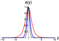
(a) The warp factor

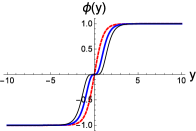
(b) The scalar field

Figure 1: The shapes of the warp factor $a(y)$ and the scalar field $\phi(y)$ of the first brane model. The parameters are set as $k=1$, $v=1$ and $n=1$ for the dashed red lines, $n=3$ for the thick blue lines, and $n=7$ for the thin black lines.

2.2 Model 2

Next we would like to construct a model with multi sub-branes, for which the warp factor has many maxima while the scalar field is still a single kink. One typical solution of such model is given by

$$\!\!\!\!a(y)\!\! =\!\! \text{sech}(k(y-b))$$ (17)

$$+\text{sech}(ky)+\text{sech}(k(y-b)),$$

$$\!\!\!\!\phi(y)\!\! =\!\! v~{}\text{tanh}(ky),$$ (18)

$$\!\!\!\!U(\phi)\!\! =\!\! \frac{k^{2}}{v^{2}}(\phi^{2}-v^{2})^{2}.$$ (19)

Here we do not show the complicate expressions of $\lambda(y)$ and $V(\phi)$. Note that $\lambda(y)$ can be solved from Eq. (11), and $V(\phi)$ is given by $V(\phi(y))=-\frac{6a^{\prime 2}}{a^{2}}-4\lambda U(\phi)$ with the replacement $y\rightarrow\frac{1}{k}{\tanh^{-1}\left({\phi}/{v}\right)}$. The shape of the warp factor of this model is shown in Fig. 2(a), from which it can be seen that small parameter $b$ corresponds to a single brane and the brane will split into three sub-branes as the parameter $b$ increases. The distance between two sub-branes is $b$.

Furthermore, this model can be extended to a brane array described by the following warp factor

$$a(y)\!\!\!\! =\!\!\!\! \sum_{n=-N}^{N}\text{sech}(k(y+nb)),$$ (20)

where $N$ is an arbitrary positive integer. Note that the above solution corresponds to the case of odd number of sub-branes. It is not difficult to construct solution for the case of even number. In addition, we only consider the simple solution for which each part of the warp factor has the same maximum.

2.3 Model 3

Finally we try to construct another kind of brane solution that will result in different effective potential for the tensor perturbation from the previous model (see the next section). In such model, there is an inner structure in the effective potential for each sub-brane. One typical solution of such brane model with double kink scalar is given by

$$a(y)\!\! =\!\! \text{tanh}[k(y+3b)]-\text{tanh}[k(y-3b)]$$ (21)

$$-\text{tanh}[k(y+b)]+\text{tanh}[k(y-b)],$$

$$\phi(y)\!\! =\!\! v\,\text{tanh}^{n}(ky),$$ (22)

$$U(\phi)\!\! =\!\! k^{2}n^{2}v^{2}\left(\frac{\phi}{v}\right)^{\frac{2(n-1)}{n}}\left[\left(\frac{\phi}{v}\right)^{\frac{2}{n}}-1\right]^{2}.$$ (23)

Here we do not show the complicate expressions of $\lambda(y)$ and $V(\phi)$. The shape of the warp factor of this model is shown in Fig. 2(b). The distance of the two sub-branes (for large $b$) is about $6b$ and the width of each sub-brane is $b$. Note that the sub-brane here is fatter than the one in the second model, which results in different structures of the effective potential for each sub-brane in the two models.

Furthermore, this model can be extended into a brane array described by the warp factor

$$a(y)\!\!\!\! = \!\!\!\!\sum_{n=-N-1}^{N}\text{tanh}\left[k(y+(2n+1)b)\right],$$ (24)

where $N$ is an arbitrary integer.

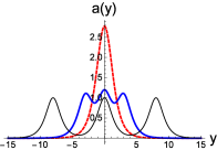
(a) model 2

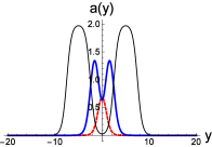
(b) model 3

Figure 2: The shape of the warp factor $a(y)$ of the brane models 2 and 3. In Fig. (a), the parameters are set as $k=1$, and $b=0.5$ for the dashed red line, $b=3$ for the thick blue line, $b=8$ for the thin black line. In Fig. (b), the parameters are set as $k=1$, and $b=0.2$ for the dashed red line, $b=0.8$ for the thick blue line, $b=2.5$ for the thin black line.

3 Tensor perturbation

In this section, we consider the linear tensor perturbation. Because of the similarity of the field equations between the mimetic gravity and general relativity, it is easy to see that the tensor perturbation is decoupled from the vector and scalar perturbations. For the tensor perturbation, the perturbed metric is given by

$$\tilde{g}_{MN}=a(y)^{2}(\eta_{\mu\nu}+h_{\mu\nu})dx^{\mu}dx^{\nu}+dy^{2},$$ (25)

where $h_{\mu\nu}=h_{\mu\nu}(x^{\mu},y)$ depends on all the coordinates and satisfies the transverse-traceless (TT) condition $\eta^{\mu\nu}\partial_{\mu}h_{\lambda\nu}=0$ and $\eta^{\mu\nu}h_{\mu\nu}=0$. The perturbation of Eq. (3) gives

$$\frac{1}{2\kappa^{2}}\delta G_{MN}+\delta\left(\lambda\partial_{M}\phi\partial_{N}\phi-\frac{1}{2}L_{\phi}g_{MN}\right)=0.$$ (26)

Using this TT condition, the perturbation of the $\mu\nu$ components of the Einstein tensor $\delta G_{\mu\nu}$ reads

$$\delta G_{\mu\nu}\!\!\!\! =\!\!\!\! -\frac{1}{2}\Box^{(4)}h_{\mu\nu}+(3a^{\prime 2}+3aa^{\prime\prime})h_{\mu\nu}$$ (27)

$$-2aa^{\prime}h^{\prime}_{\mu\nu}-\frac{1}{2}a^{2}h^{\prime\prime}_{\mu\nu},$$

where the four-dimensional d’Alembertian is defined as $\Box^{(4)}\equiv\eta_{\mu\nu}\partial_{\mu}\partial_{\nu}$. Using Eqs. (7) and (27), the above equation reads

$$-\frac{1}{2}\Box^{(4)}h_{\mu\nu}-2aa^{\prime}h^{\prime}_{\mu\nu}-\frac{1}{2}a^{2}h^{\prime\prime}_{\mu\nu}=0.$$ (28)

After redefining the extra dimension coordinate $dz=\frac{1}{a(z)}dy$ and the pertubation $h_{\mu\nu}=a(z)^{-\frac{3}{2}}\tilde{h}_{\mu\nu}$, we get the equation of $\tilde{h}_{\mu\nu}$:

$$\Box^{(4)}\tilde{h}_{\mu\nu}+\partial^{2}_{z}\tilde{h}_{\mu\nu}-\frac{\partial^{2}_{z}a^{\frac{3}{2}}}{a^{\frac{3}{2}}}\tilde{h}_{\mu\nu}=0.$$ (29)

Considering the decomposition $\tilde{h}_{\mu\nu}=\epsilon_{\mu\nu}(x^{\gamma})\text{e}^{ip_{\lambda}x^{\lambda}}t(z)$, where the polarization tensor $\epsilon_{\mu\nu}$ satisfies the TT condition $\eta^{\mu\nu}\partial_{\mu}\epsilon_{\lambda\nu}=0$ and $\eta^{\mu\nu}\epsilon_{\mu\nu}=0$, we obtain the Schrödinger-like equation for $t(z)$:

$$-\partial^{2}_{z}t(z)+V_{t}(z)t(z)=m_{t}^{2}t(z),$$ (30)

with the potential $V_{t}(z)$ given by

$$V_{t}(z)=\frac{\partial^{2}_{z}a^{\frac{3}{2}}}{a^{\frac{3}{2}}}.$$ (31)

Now we can see that the equation of the tensor perturbation in mimetic gravity is the same as that in general relativity. Nevertheless, the mimetic scalar field generates more types of thick brane, which could lead to new type of potential of the tensor perturbation. We present the potentials of the tensor perturbations for three models in Figs. 3 - 5, respectively. In model 1, the potential is a volcano-like potential. As the parameter $n$ increases, the potential well become narrower and deeper. In model 2, as the parameter $b$ increases, the single brane splits into three sub-branes, and the volcano-like potential changes to a tri-well potential, and at last splits into three independent volcano-like potentials. In model 3, as the parameter $b$ increases, the single potential well splits into a double-well, and then becomes two volcano-like potentials with inner structure. For both cases, the distance of the those wells increases with $b$.

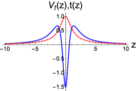
(a)  $n=1$

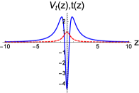
(b)  $n=3$

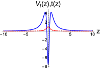
(c)  $n=5$

Figure 3: The effective potential $V_{t}(z)$ (blue solid lines) and the zero mode $t_{0}(z)$ (red dashed lines) of the tensor perturbation for brane model 1. The parameters are set as $k=1$, and $n=1$ in Fig. (a), $n=3$ in Fig. (b), $n=5$ in Fig. (c).

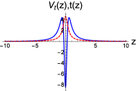
(a)  $b=0.5$

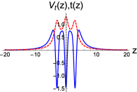
(b)  $b=3$

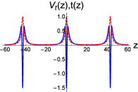
(c)  $b=8$

Figure 4: The effective potential $V_{t}(z)$ (blue solid lines) and the zero mode $t_{0}(z)$ (red dashed lines) of the tensor perturbation for brane model 2. The parameters are set as $k=1$, and $b=0.5$ in Fig. (a), $b=3$ in Fig. (b), $b=8$ in Fig. (c).

The zero mode of the tensor perturbation is

$$t_{0}(z)\propto a^{\frac{3}{2}}(z).$$ (32)

It is easy to verify that the zero modes for the above brane models are square-integrable and hence are localized around the brane. Thus the four-dimensional Newtonian potential can be realized on the brane. Also Eq. (30) can be factorized as

$$\left(-\partial_{z}+\frac{\partial_{z}a^{\frac{3}{2}}}{a^{\frac{3}{2}}}\right)\left(\partial_{z}+\frac{\partial_{z}a^{\frac{3}{2}}}{a^{\frac{3}{2}}}\right)t(z)=m_{t}^{2}t(z).$$ (33)

It is clear that there is no tensor tachyon mode, thus the brane is stable against the tensor perturbation.

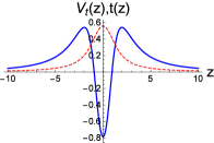
(a)  $a=0.2$

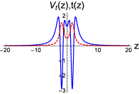
(b)  $b=0.8$

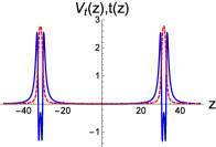
(c)  $b=2.5$

Figure 5: The effective potential $V_{t}(z)$ (blue solid lines) and the zero mode $t_{0}(z)$ (red dashed lines) of the tensor perturbation for brane model 3. The parameters are set as $k=1$, and $a=0.2$ in Fig. (a), $b=0.8$ in Fig. (b), $b=2.5$ in Fig. (c).

4 Scalar perturbation

In this section, we study the scalar pertubation. The perturbed metric is

$$ds^{2}=a^{2}(z)\left[(1+2\psi)\eta_{\mu\nu}dx^{\mu}dx^{\nu}+(1+2\Phi)dz^{2}\right].$$ (34)

From Eq. (3) we have

$$R_{MN}+2\lambda\partial_{M}\phi\partial_{N}\phi-\frac{2}{3}g_{MN}(\lambda U+V)=0.$$ (35)

The perturbation of Eq. (35) reads

$$\delta R_{\mu\nu}-\frac{4}{3}(\partial_{z}a)^{2}\psi(\lambda U+V)\eta_{\mu\nu}$$

$$-\frac{2}{3}a^{2}\eta_{\mu\nu}\left(\lambda\frac{\partial U}{\partial\phi}\delta\phi+\frac{\partial V}{\partial\phi}\delta\phi\right)=0,$$ (36)

$$\delta R_{\mu 5}+2\lambda\partial_{z}\phi\partial_{\mu}\delta\phi=0,$$ (37)

$$\delta R_{55}+4\lambda\partial_{z}\phi\delta\partial_{z}\phi-\frac{2}{3}a^{2}\left(\lambda\frac{\partial U}{\partial\phi}\delta\phi+\frac{\partial V}{\partial\phi}\delta\phi\right)$$

$$-\frac{4}{3}a^{2}(\lambda U+V)\Phi=0,$$ (38)

where the components of $\delta R_{MN}$ are given by

$$\delta R_{\mu\nu}\!\!\! = \!\!\!-2\partial_{\mu}\partial_{\nu}\psi-\partial_{\mu}\partial_{\nu}\Phi-\eta_{\mu\nu}\Box^{(4)}\psi-\eta_{\mu\nu}\partial^{2}_{z}\psi,$$ (39)

$$\!\!\!\!\!\!+\left(\frac{4(\partial_{z}a)^{2}}{a^{2}}+\frac{2\partial^{2}_{z}a}{a}\right)(\Phi-\psi)\eta_{\mu\nu}$$

$$+\frac{\partial_{z}a}{a}(\partial_{z}\phi-7\partial_{z}\psi)\eta_{\mu\nu},$$

$$\delta R_{\mu 5}\!\!\! = \!\!\!\partial_{\mu}\left(\frac{3\partial_{z}a}{a}\Phi-3\partial_{z}\psi\right),$$ (40)

$$\delta R_{55}\!\!\! = \!\!\!-\Box^{(4)}\Phi-4\partial^{2}_{z}\psi+\frac{4\partial_{z}a}{a}(\partial_{z}\phi-\partial_{z}\psi).$$ (41)

On the other hand, the perturbation of Eq. (5) gives

$$\frac{2}{a^{2}}\partial_{z}\phi\partial_{z}\delta\phi-\frac{2}{a^{2}}(\partial_{z}\phi)^{2}\Phi=\frac{\partial U}{\partial\phi}\delta\phi,$$ (42)

which follows that

$$\Phi=\frac{\partial_{z}\delta\phi}{\partial_{z}\phi}-\frac{a^{2}}{2(\partial_{z}\phi)^{2}}\frac{\partial U}{\partial\phi}\delta\phi.$$ (43)

From the off-diagonal part of Eq. (39) we get the simple relation between the scalar modes $\Phi$ and $\psi$ in the perturbation of the metric:

$$\Phi=-2\psi.$$ (44)

Substituting Eqs. (43) and (44) into Eq. (37) and integrating with respect to the four-dimensional coordinates $x^{\mu}$, we get the master equation of the scalar perturbation $\delta\phi$

$$\!\!\!\!\!\!\!\!\!\!\!\!\!\!\!\!\!\!\!\!\!\!\!\!-\frac{3}{2}\partial^{2}_{z}\delta\phi+\frac{3}{4}\left(\frac{a^{2}}{\partial_{z}\phi}\frac{\partial U}{\partial\phi}+\frac{2\partial^{2}_{z}\phi}{\partial_{z}\phi}-\frac{4\partial_{z}a}{a}\right)\partial_{z}\delta\phi$$

$$\!\!\!\!\!\!\!\!\!\!\!\!\!\!\!\!\!\!\!\!\!\!\!\!\!\!\!\!\!\!\!\!\!\!+\!\left[\frac{3a\partial_{z}a}{\partial_{z}\phi}\frac{\partial U}{\partial\phi}\!\!+\!\!2\lambda(\partial_{z}\phi)^{2}\!\!+\!\!\frac{3}{4}a^{2}\left(\frac{\partial^{2}U}{\partial\phi^{2}}\!-\!2\frac{\partial U}{\partial\phi}\frac{\partial^{2}_{z}\phi}{(\partial_{z}\phi)^{2}}\right)\right]\!\delta\phi\!\!=\!\!0.$$ (45)

To simplify this equation, we have to use the background equations (3)-(5) in the coordinate system ($x^{\mu},z$),

$$\!\!\!\!\!\!\!\!\!\!\!\!\frac{3a^{\prime\prime}}{a^{3}}=-V(\phi),$$ (46)

$$\!\!\!\!\!\!\!\!\!\!\!\!\frac{6a^{\prime 2}}{a^{2}}+a^{2}V(\phi)+2a^{2}\lambda U(\phi)=0,$$ (47)

$$a^{2}(\lambda U^{\prime}(\phi)+\frac{\partial V}{\partial\phi})+6\lambda\partial_{z}\phi\frac{a^{\prime}}{a}+2\lambda^{\prime}\partial_{z}\phi$$

$$+2\lambda\partial^{2}_{z}\phi=0,$$ (48)

$$\!\!\!\!\!\!\!\!\!\!\!\!\frac{1}{a^{2}}(\partial_{z}\phi)^{2}=U(\phi),$$ (49)

and redefine $\delta\phi(x^{\mu},z)=\frac{(\partial_{z}\phi)^{\frac{3}{2}}}{a^{2}}s(z)\overline{\delta\phi}(x^{\mu})$. Then Eq. (4) turns to

$$-\partial^{2}_{z}s(z)+V_{s}(z)s(z)=0,$$ (50)

with the effective potential $V_{s}(z)$ given by

$$V_{s}(z)=\frac{2(\partial_{z}a)^{2}-a\partial^{2}_{z}a}{a^{2}}+\frac{-(\partial^{2}_{z}\phi)^{2}+2\partial_{z}\phi\partial^{3}_{z}\phi}{4(\partial_{z}\phi)^{2}}.$$ (51)

The corresponding scalar perturbation mode in the metric is given by Eqs. (43) and (44).

Note that there is no term of the form $\Box^{4}\delta\phi$ in Eq. (4), and hence there is no term of the form $m_{s}^{2}s(z)$ in Eq. (50), which is consistent with the cosmological scalar perturbation in mimetic gravity [2]. This implies that the scalar perturbations do not propagate on the brane. Thus there is no tachyon scalar mode, and the brane is stable under the linear scalar perturbations.

The effective potential $V_{s}(z)$ for the three models are shown in Figs. 6 - 8, respectively. From these figures, it can be seen that, for model 1, there are two wells for the parameter $n=1$ and $n=3$, while when $n=5$ there are three, and the potential is divergent at the origin; for model 2, the potential turns from a double-well into four sub-wells as the parameter $b$ increases; for model 3, the potential remains a double-well as the parameter $b$ increases. Furthermore, for all the three brane models, the potential approaches $0^{-}$ at infinity, hence the scalar perturbations are not localized on the brane and would not lead to the “fifth force”.

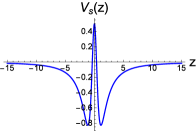
(a)  $n=1$

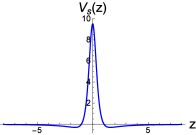
(b)  $n=3$

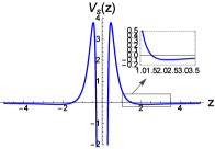
(c)  $n=5$

Figure 6: The effective potential $V_{s}(z)$ for model 1. The parameters are set as $k=1$, $v=1$ and $n=1$ in Fig. (a), $n=3$ in Fig. (b), $n=5$ in Fig. (c).

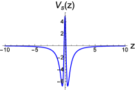
(a)  $b=0.5$

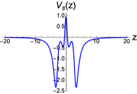
(b)  $b=3$

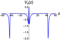
(c)  $b=8$

Figure 7: The effective potential $V_{s}(z)$ for model 2. The parameters are set as $k=1$, $v=1$ and $b=0.5$ in Fig. (a), $b=3$ in Fig. (b), $b=8$ in Fig. (c).

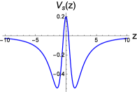
(a)  $a=0.2$

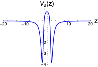
(b)  $b=0.8$

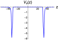
(c)  $b=2.5$

Figure 8: The effective potential $V_{s}(z)$ of the model 3. The parameters are set as $k=1$, $v=1$, $n=1$, and $a=0.2$ in Fig. (a), $b=0.8$ in Fig. (b), $b=2.5$ in Fig. (c).

5 Conclusion

In this work, we investigated three kinds of thick branes generated by the mimetic scalar field, which represents the isolated conformal degree of freedom. Since we are free to choose arbitrary potentials $V(\phi)$ and $U(\phi)$, it is possible to construct abundant kinds of thick brane models in mimetic gravity. In the first brane model, we get a single brane with a double-kink scalar field. In the last two brane models, the branes split into many sub-branes as the parameter $b$ increases, and the potentials $V_{t}(z)$ and $V_{s}(z)$ of the extra parts $t(z)$ and $s(z)$ of the tensor and scalar perturbations also split into multi-wells. We also showed that the branes are stable under the tensor perturbations and the Newtonian potentials can be realized on the branes. The scalar perturbations do not propagate on the brane, which is quite different from other brane models. By analyzing the potential $V_{s}(z)$ we conclude that the scalar perturbations $s(z)$ for the three models are not localized on the brane.

Furthermore, models 2 and 3 can be extended into the case of brane array. The inner structure of the brane may lead to new phenomenon in the resonance of the tensor perturbation and the localization of matter fields. We will consider this issue in the future work.

References

- [1] A. H. Chamseddine and V. Mukhanov, Mimetic Dark Matter, JHEP 11 (2013) 135, [arXiv:1308.5410].
- [2] A. H. Chamseddine, V. Mukhanov and A. Vikman, Cosmology with Mimetic Matter, JCAP 1406 (2014) 017, [arXiv:1403.3961].
- [3] S. Nojiri and S. D. Odintsov, Mimetic f(R) gravity: Inflation, dark energy and bounce, Modern Physics Letters A 29 (dec, 2014) 1450211, [arXiv:1408.3561].
- [4] D. Momeni, R. Myrzakulov and E. Güdekli, Cosmological viable mimetic and theories via Noether symmetry, Int. J. Geom. Meth. Mod. Phys. 12 (2015) 1550101, [arXiv:1502.00977].
- [5] S. D. Odintsov and V. K. Oikonomou, Viable Mimetic Gravity Compatible with Planck Observations, Annals Phys. 363 (2015) 503–514, [arXiv:1508.07488].
- [6] S. D. Odintsov and V. K. Oikonomou, Mimetic inflation confronted with Planck and BICEP2/Keck Array data, Astrophys. Space Sci. 361 (2016) 174, [arXiv:1512.09275].
- [7] J. Matsumoto, S. D. Odintsov and S. V. Sushkov, Cosmological perturbations in a mimetic matter model, Phys. Rev. D91 (2015) 064062, [arXiv:1501.02149].
- [8] S. Nojiri, S. D. Odintsov and V. K. Oikonomou, Unimodular-Mimetic Cosmology, Class. Quant. Grav. 33 (2016) 125017, [arXiv:1601.07057].
- [9] S. D. Odintsov and V. K. Oikonomou, Accelerating cosmologies and the phase structure of F(R) gravity with Lagrange multiplier constraints: A mimetic approach, Phys. Rev. D93 (2016) 023517, [arXiv:1511.04559].
- [10] V. K. Oikonomou, Reissner-Nordström Anti-de Sitter Black Holes in Mimetic Gravity, Universe 2 (2016) 10, [arXiv:1511.09117].
- [11] G. Cognola, R. Myrzakulov, L. Sebastiani, S. Vagnozzi and S. Zerbini, Covariant renormalizable gravity model as a mimetic Horndeski model: cosmological solutions and perturbations, arXiv:1601.00102.
- [12] Y. Rabochaya and S. Zerbini, A note on a mimetic scalar–tensor cosmological model, Eur. Phys. J. C76 (feb, 2016) .
- [13] S. D. Odintsov and V. K. Oikonomou, Unimodular Mimetic Inflation, Astrophys. Space Sci. 361 (2016) 236, [arXiv:1602.05645].
- [14] L. Sebastiani, S. Vagnozzi and R. Myrzakulov, Mimetic gravity: a review of recent developments and applications to cosmology and astrophysics, Adv. High Energy Phys. 2017 (2017) 3156915, [arXiv:1612.08661].
- [15] L. Randall and R. Sundrum, A Large mass hierarchy from a small extra dimension, Phys. Rev. Lett. 83 (1999) 3370–3373, [arXiv:hep-ph/9905221].
- [16] L. Randall and R. Sundrum, An Alternative to compactification, Phys. Rev. Lett. 83 (1999) 4690–4693, [arXiv:hep-th/9906064].
- [17] J. E. Kim, B. Kyae and H. M. Lee, Randall-Sundrum model for selftuning the cosmological constant, Phys. Rev. Lett. 86 (2001) 4223–4226, [arXiv:hep-th/0011118].
- [18] H. Davoudiasl, J. L. Hewett and T. G. Rizzo, Bulk gauge fields in the Randall-Sundrum model, Phys. Lett. B473 (2000) 43–49, [arXiv:hep-ph/9911262].
- [19] T. Shiromizu, K.-i. Maeda and M. Sasaki, The Einstein equation on the 3-brane world, Phys. Rev. D62 (2000) 024012, [arXiv:gr-qc/9910076].
- [20] T. Gherghetta and A. Pomarol, Bulk fields and supersymmetry in a slice of AdS, Nucl. Phys. B586 (2000) 141–162, [arXiv:hep-ph/0003129].
- [21] T. G. Rizzo, Introduction to Extra Dimensions, AIP Conf. Proc. 1256 (2010) 27–50, [arXiv:1003.1698].
- [22] K. Yang, Y.-X. Liu, Y. Zhong, X.-L. Du and S.-W. Wei, Gravity localization and mass hierarchy in scalar-tensor branes, Phys. Rev. D86 (2012) 127502, [arXiv:1212.2735].
- [23] K. Agashe, A. Azatov, Y. Cui, L. Randall and M. Son, Warped Dipole Completed, with a Tower of Higgs Bosons, JHEP 06 (2015) 196, [arXiv:1412.6468].
- [24] C. Csaki, J. Erlich, T. J. Hollowood and Y. Shirman, Universal aspects of gravity localized on thick branes, Nucl. Phys. B581 (2000) 309–338, [arXiv:hep-th/0001033].
- [25] O. DeWolfe, D. Z. Freedman, S. S. Gubser and A. Karch, Modeling the fifth-dimension with scalars and gravity, Phys. Rev. D62 (2000) 046008, [arXiv:hep-th/9909134].
- [26] M. Gremm, Four-dimensional gravity on a thick domain wall, Phys. Lett. B478 (2000) 434–438, [arXiv:hep-th/9912060].
- [27] Y.-X. Liu, Introduction to Extra Dimensions and Thick Braneworlds, arXiv:1707.08541.
- [28] N. Sadeghnezhad and K. Nozari, Braneworld Mimetic Cosmology, Phys. Lett. B769 (2017) 134–140, [arXiv:1703.06269].
- [29] V. I. Afonso, D. Bazeia and L. Losano, First-order formalism for bent brane, Phys. Lett. B634 (2006) 526–530, [arXiv:hep-th/0601069].
- [30] V. Afonso, D. Bazeia, R. Menezes and A. Y. Petrov, f(R)-Brane, Phys.Lett. B658 (2007) 71–76, [arXiv:0710.3790].
- [31] B. Guo, Y.-X. Liu and K. Yang, Brane worlds in gravity with auxiliary fields, Eur. Phys. J. C75 (2015) 63, [arXiv:1405.0074].
- [32] G. German, A. Herrera-Aguilar, D. Malagon-Morejon, I. Quiros and R. da Rocha, Study of field fluctuations and their localization in a thick braneworld generated by gravity non-minimally coupled to a scalar field with a Gauss-Bonnet term, Phys. Rev. D89 (2014) 026004, [arXiv:1301.6444].
- [33] Y.-X. Liu, Y. Zhong and K. Yang, Scalar-Kinetic Branes, EPL 90 (2010) 51001, [arXiv:0907.1952].
- [34] V. Dzhunushaliev, V. Folomeev and M. Minamitsuji, Thick brane solutions, Rept. Prog. Phys. 73 (2010) 066901, [arXiv:0904.1775].
- [35] O. Arias, R. Cardenas and I. Quiros, Thick brane worlds arising from pure geometry, Nucl. Phys. B643 (2002) 187–200, [arXiv:hep-th/0202130].
- [36] N. Barbosa-Cendejas and A. Herrera-Aguilar, Localization of 4-D gravity on pure geometrical thick branes, Phys. Rev. D73 (2006) 084022, [arXiv:hep-th/0603184].
- [37] H. Liu, H. Lu and Z.-L. Wang, f(R) Gravities, Killing Spinor Equations, ’BPS’ Domain Walls and Cosmology, JHEP 02 (2012) 083, [arXiv:1111.6602].
- [38] V. Dzhunushaliev, V. Folomeev, B. Kleihaus and J. Kunz, Some thick brane solutions in f(R)-gravity, JHEP 04 (2010) 130, [arXiv:0912.2812].
- [39] Y. Zhong and Y.-X. Liu, Pure geometric thick -branes: stability and localization of gravity, Eur. Phys. J. C76 (2016) 321, [arXiv:1507.00630].
- [40] A. V. Astashenok, S. D. Odintsov and V. K. Oikonomou, Modified Gauss-Bonnet gravity with the Lagrange multiplier constraint as mimetic theory, Class. Quant. Grav. 32 (2015) 185007, [arXiv:1504.04861].