Hypostatic jammed packings of frictionless nonspherical particles

Abstract

We perform computational studies of static packings of a variety of nonspherical particles including circulo-lines, circulo-polygons, ellipses, asymmetric dimers, dumbbells, and others to determine which shapes form packings with fewer contacts than degrees of freedom (hypostatic packings) and which have equal numbers of contacts and degrees of freedom (isostatic packings), and to understand why hypostatic packings of nonspherical particles can be mechanically stable despite having fewer contacts than that predicted from naïve constraint counting. To generate highly accurate force- and torque-balanced packings of circulo-lines and -polygons, we developed an interparticle potential that gives continuous forces and torques as a function of the particle coordinates. We show that the packing fraction and coordination number at jamming onset obey a master-like form for all of the nonspherical particle packings we studied when plotted versus the particle asphericity ${\cal A}$, which is proportional to the ratio of the squared perimeter to the area of the particle. Further, the eigenvalue spectra of the dynamical matrix for packings of different particle shapes collapse when plotted at the same ${\cal A}$. For hypostatic packings of nonspherical particles, we verify that the number of “quartic” modes along which the potential energy increases as the fourth power of the perturbation amplitude matches the number of missing contacts relative to the isostatic value. We show that the fourth derivatives of the total potential energy in the directions of the quartic modes remain nonzero as the pressure of the packings is decreased to zero. In addition, we calculate the principal curvatures of the inequality constraints for each contact in circulo-line packings and identify specific types of contacts with inequality constraints that possess convex curvature. These contacts can constrain multiple degrees of freedom and allow hypostatic packings of nonspherical particles to be mechanically stable.

I Introduction

There have been a significant number of computational studies aimed at elucidating the jamming transition in static packings of frictionless spherical particles O’Hern et al. (2003); Liu and Nagel (2010); van Hecke (2009). Key findings from these studies include: i) sphere packings at jamming onset at packing fraction $\phi_{J}$ are isostatic (where the number of contacts matches the number of degrees of freedom, as shown in Fig. 1), ii) the coordination number, shear modulus, and other structural and mechanical quantities display power-law scaling as a function of the system’s pressure $P$ as packings are compressed above jamming onset at $P=0$, and iii) the density of vibrational modes develops a plateau at low frequencies $\omega$ that extends toward $\omega\rightarrow 0$ as the system approaches jamming onset. Many of these results are robust with respect to changes in the particle size polydispersity and different forms for the purely repulsive interparticle potential.

Most studies of jamming to date have been performed on packings of disks in 2D or spheres in 3D. More recently, both computational and experimental studies have begun focusing on packings of nonspherical shapes, such as ellipsoids Donev et al. (2007); Mailman et al. (2009); Schreck et al. (2012); Zeravcic et al. (2009); Basavaraj et al. (2006); Schaller et al. (2015); Donev et al. (2004); Man et al. (2005), spherocylinders Zhao et al. (2012); Blouwolff and Fraden (2006); Williams and Philipse (2003); Meng et al. (2016); Wouterse et al. (2007, 2009), polyhedra Jiao and Torquato (2011); Chen et al. (2014), and composite particles Schreck et al. (2010); Gaines et al. (2017); Miskin and Jaeger (2013); Baule et al. (2013). In particular, there is a well-established set of results on packings of frictionless ellipses (or ellipsoids in 3D). In general, static packings of frictionless ellipses are hypostatic with fewer contacts than the number of degrees of freedom using naïve contact counting. For amorphous mechanically stable (MS) packings of disks, the coordination number in the large-system limit is $z=2d_{f}$ (where $d_{f}=2$ is the number of degrees of freedom per particle) Tkachenko and Witten (1999). Thus, one might expect that the coordination number for ellipses in 2D would jump from $z=4$ to $z=6$ (with $d_{f}=3$) for any aspect ratio $\alpha>1$. However, $z(\alpha)$ increases continuously from $4$ at $\alpha=1$ and remains less than $6$ for all $\alpha$. We have shown that the number of missing contacts exactly matches the number of “quartic” eigenmodes from the dynamical matrix for which the potential energy increases as the fourth power of the displacement for perturbations along the corresponding eigenmode Schreck et al. (2012). In addition, the packing fraction at jamming onset $\phi_{J}(\alpha)$ possesses a peak near $\alpha\approx 1.5$, and then decreases for increasing $\alpha$.

Are these results for ellipses similar to those for all other nonspherical or elongated particle shapes? Prior results for packings of spherocylinders have shown that they are hypostatic Wouterse et al. (2007). However, packings of composite particles formed from collections of disks (2D) Schreck et al. (2010); Papanikolaou et al. (2013) or spheres (3D) Gaines et al. (2017) are isostatic at jamming onset. Unfortunately, very few studies explicitly check whether hypostatic packings are mechanically stable. The goal of this article is to determine which particle shapes can form mechanically stable (i.e. jammed), hypostatic packings, identify a key shape parameter that controls the forms of the coordination number $z$ and packing fraction $\phi_{J}$, and gain a fundamental understanding for why hypostatic packings are mechanically stable, even at jamming onset $P=0$.

To address these questions, we generate static packings using a compression and decompression scheme coupled with energy minimization for nine different convex particle shapes (ellipses, circulo-lines, circulo-triangles, circulo-pentagons, circulo-octogons, circulo-decagons Wang et al. (2015), dimers Schreck et al. (2010), dumbbells Han and Kim (2012), and Reuleaux triangles Atkinson et al. (2012)) in 2D. To study such a wide range of particle shapes, we developed a fully continuous and differentiable interparticle potential for circulo-lines and circulo-polygons, which allows us to generate packings with extremely accurate force and torque balance at very low pressure. We find several important results. First, we show that the jammed packing fraction for the nine particle shapes collapses onto a master-like curve when plotted versus the asphericity parameter ${\cal A}=p^{2}/4\pi a$, where $p$ is the perimeter and $a$ is the area of the particle. We also show that the coordination number $z({\cal A})$ follows a master-like curve when contacts between nearly parallel circulo-lines or nearly parallel sides of circulo-polygons are treated properly. In addition, for packings of circulo-lines, we calculate the fourth derivatives of the total potential energy along the quartic modes of the dynamical matrix Schreck et al. (2012) and show that the fourth derivatives are nonzero as $P\rightarrow 0$, which proves that these hypostatic packings are mechanically stable. Finally, we calculate the principal curvatures of the constraint surfaces in configuration space defined by each contact to identify which types of contacts in packings of circulo-lines allow them to be mechanically stable, while hypostatic.

Figure 1: An isostatic packing of $N=18$ bidisperse disks ($9$ large and $9$ small with diameter ratio $r=1.4$) in a square box with periodic boundary conditions at jamming onset $\phi_{J}=0.835$. Blue disks form the force-bearing backbone, and red disks are “rattler” disks that possess fewer than $3$ contacts. This isostatic packing possesses $N_{c}=N_{c}^{0}=2(N-N_{r})-1=31$ contacts, where $N_{c}^{0}$ is the isostatic number of contacts.

This article is organized as follows. In Sec. II, we describe the compression and decompression plus minimization method we use to generate static packings of convex, nonspherical particles. In Sec. III.1, we present examples of static packings of several different convex, nonspherical particle shapes to put forward a conjecture concerning which nonspherical particle shapes form hypostatic packings and which always form isostatic packings. In Sec. III.2, we show that the packing fraction at jamming onset $\phi({\cal A})$ and coordination number $z({\cal A})$ display master-like forms when plotted versus the particle asphericity ${\cal A}$, for nine different nonspherical particle shapes. In this section, we also show results for the calculations of the fourth derivatives of the total potential of the static packings in the directions of dynamical matrix eigenmodes. Finally, in Sec. III.3, we calculate and analyze the principal curvatures of the constraint surfaces given by the interparticle contacts to understand the grain-scale mechanisms that enable hypostatic packings to be mechanically stable. We also include three Appendices. Appendix A describes the development of a continuous interparticle repulsive potential between circulo-lines and circulo-polygons, which allows us to generate extremely accurate force- and torque-balanced jammed packings near zero pressure. Appendix B describes how we generate different circulo-polygon shapes at constant asphericity ${\cal A}$. Finally, in Appendix C, we provide expressions for the elements of the dynamical matrix for packings of circulo-polygons.

II Methods

Table 1: A list of the nine convex, nonspherical particle shapes studied in this article, along with the ranges of aspect ratio $\alpha$ and asphericity ${\cal A}$ that we considered.

Particle Shape	$\alpha-1$	${\cal A}-1$
Circulo-Line	$10^{-3}$ – $4$	$4.05\times 10^{-7}$ – $1.06$
Circulo-Triangle	–	$10^{-6.5}$ – $0.4$
Circulo-Pentagon	–	$10^{-6.5}$ – $0.4$
Circulo-Octagon	–	$10^{-6.5}$ – $0.4$
Circulo-Decagon	–	$10^{-6.5}$ – $0.1$
Dimer	$0.571$	$0.349$
Dumbbell	$2$ – $4$	$0.514$ – $2.405$
Reuleaux Triangle	–	$0.114$
Ellipse	$10^{-4}$ – $0.9$	$3.75\times 10^{-9}$ – $0.161$

Using computer simulations, we generate static packings of frictionless, nonspherical, convex particles in 2D. The particles are nearly hard in the sense that we consider mechanically stable packings in the zero-pressure limit. We study nine different particle shapes: circulo-lines, circulo-triangles, circulo-pentagons, circulo-octagons, circulo-decagons, Reuleaux triangles, ellipses, dumbbells, and dimers. (See Table 1.) We focus on bidisperse mixtures in which half of the particles are large and half are small to prevent crystallization Speedy (1998); O’Hern et al. (2003). The large particles have areas that satisfy $a_{L}=1.4^{2}a_{S}$, where $a_{L,S}$ is the area of the large and small particles, respectively. Both particles have the same mass, $m$. We generated static packings at fixed asphericity ${\cal A}$ for the large and small particles over a wide range of ${\cal A}$. We employ periodic boundary conditions in square domains with edge length $L=1$ and system sizes that vary from $N=24$ to $480$ particles. Note that the term “convex particle shapes” stands for “shapes whose accessible contact surface is nowhere locally concave.” Our studies include dimers (which possess two points on the surface that are concave), circulo-lines (which contain regions of zero curvature), ellipses, and other explicitly convex particles.

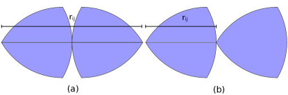
Figure 2: Definition of the separation $r_{ij}$ between two Reuleaux triangles when (a) the two circular arcs are overlapping and (b) a vertex is overlapping one of the circular arcs. In case (a), $r_{ij}$ is the distance between the vertices at the centers of the corresponding arcs. In case (b), $r_{ij}$ is the distance between the arc’s central vertex and the vertex overlapping the arc.

We assume that particles $i$ and $j$ interact via the purely repulsive, pairwise linear spring potential,

$$U(r_{ij})=\frac{k}{2}\left(\sigma_{ij}-r_{ij}\right)^{2}\Theta\left(\sigma_{ij}-r_{ij}\right),$$ (1)

where $k$ is the spring constant of the interaction and $\Theta(x)$ is the Heaviside step function. Below, lengths, energies, and pressures will be expressed in units of $L$, $kL^{2}$, and $k$, respectively. For disks, $r_{ij}$ is the separation between the centers of disks $i$ and $j$, and $\sigma_{ij}=R_{i}+R_{j}$ is the sum of the radii of disks $i$ and $j$.

For dimers, i.e. composite particles formed from two circular monomers, $r_{ij}$ is the center-to-center separation between each pair of interacting monomers, and $\sigma_{ij}$ is the sum of the radii of those monomers. A Reuleaux triangle is a shape that is constructed by joining three circular arcs of equal radius such that their intersection points (vertices of the Reuleaux triangle) are the centers of each circle. For this shape, we first identify whether two arcs are overlapping or whether a vertex is overlapping an arc. We then set $r_{ij}$ in Eq. 1 to be the distance between the center points of the overlapping arcs (in the case of two overlapping arcs) or the distance between the center point of the arc and the vertex (in the case of a vertex overlapping an arc). We set $\sigma_{ij}$ to be the sum of the radii of the two overlapping arcs, or the radius of the single arc when a vertex is overlapping an arc. (See Fig. 2.)

For ellipses, we take $r_{ij}$ to be the distance between the centers of the particles, and $\sigma_{ij}$ to be the center-center distance that would bring the particles exactly into contact at their current orientations Schreck et al. (2012). For dumbbell-shaped particles, we have multiple possible cases for $r_{ij}$, depending on their orientations. We calculate $r_{ij}$ either as the distance between each pair of circular ends, or between each circular end and the other particle’s shaft, with $\sigma_{ij}$ chosen to be the sum of the relevant radii in each case. The repulsive contact interactions between circulo-lines and -polygons are calculated in a similar fashion to dumbbells. However, because the regions of changing curvature in the case of circulo-lines and -polygons are accessible, unlike in the dumbbell case, additional constraints in the potential are necessary to prevent discontinuities in the pairwise torques and forces. For a thorough explanation of how we define a continuous, repulsive linear spring potential between circulo-lines and polygons, see Appendix A.

To generate static packings, we successively compress and decompress the system with each compression or decompression step followed by the conjugate gradient method to minimize the total potential energy $U=\sum_{i>j}U(r_{ij})$. We use a binary search algorithm to push the system to a target pressure $P=P_{0}$. If $P>P_{0}$, the system is decompressed isotropically, and if $P<P_{0}$, the system is compressed isotropically. Subsequently, we perform minimization of the enthalpy Smith et al. (2014) $H=U+P_{0}A$, where $A$ is the area of the system, the pressure $P=-dU/dA$, and $P_{0}=10^{-9}$ is the target pressure, with the particle positions and the box edge length as the degrees of freedom. Using this algorithm, we achieve accurate force and torque balance such that the squared forces $f^{2}_{i}$ and torques $\tau_{i}^{2}$ on a given particle $i$ do not exceed $10^{-25}$.

After generating each static packing, we calculate its dynamical matrix $M$, which is the Hessian matrix of second derivatives of the total potential energy $U$ with respect to the particle coordinates:

$$M_{ij}=\frac{\partial^{2}U}{\partial\xi_{i}\partial\xi_{j}},$$ (2)

where $\xi_{i}=x_{i}$, $y_{i}$, and $\theta_{i}$, $x_{i}$ and $y_{i}$ are the coordinates of the geometric center of particle $i$, and $\theta_{i}$ characterizes the rotation angle of particle $i$. We then calculate the $3N$ eigenvalues $\lambda_{i}$ of $M$, and the corresponding eigenvectors ${\vec{\lambda}}_{i}$ with ${\vec{\lambda}}^{2}_{i}=1$. For more details on the calculation of the dynamical matrix elements, see Appendix C.

III Results

Our results are organized into three subsections. In Sec. III.1, we discuss which nonspherical particle shapes give rise to hypostatic packings, and then propose specific criteria that nonspherical particle shapes must satisfy to yield hypostatic packings. In Sec. III.2, we show the variation of the packing fraction $\phi$ and coordination number $z$ at jamming onset with particle asphericity ${\cal A}$ for packings of circulo-lines, circulo-polygons, and ellipses. Finally, in Sec. III.3, we calculate the principal curvatures of the inequality constraints in configuration space arising from interparticle contacts for hypostatic packings of circulo-lines to identify the specific types of contacts that allow static packings to be hypostatic, yet mechanically stable.

III.1 Nonspherical Particle Shapes that Give Rise to Hypostatic Packings

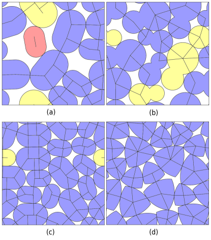
Figure 3: Two isostatic ((a) and (b)) and two hypostatic packings ((c) and (d)) of nonspherical particles. (a) This packing with $\phi=0.782$ consists of $10$ non-rotating circulo-lines with asphericity ${\cal A}=1.06$. The red particle is a rattler with two unconstrained degrees of freedom, and the yellow particle is a slider with one unconstrained degree of freedom. The blue and yellow particles form an isostatic contact network with $N_{c}=2N-4=16$ contacts, where we have subtracted off $3$ additional contacts due to the rattler and slider particles. (b) This packing with $\phi=0.828$ consists of $10$ asymmetric dimers. The two monomers on a given dimer have a diameter ratio $r=1.4$ and the ratio of the lengths of large and small dimer axes is $d=1.4$. The three yellow ‘rotator’ particles each have one unconstrained rotational degree of freedom. The particles form an isostatic contact network with $N_{c}=3N-4=26$, where we have subtracted off $3$ additional contacts due to the rotator particles. (c) This packing with $\phi=0.892$ consists of $18$ rotating circulo-lines with asphericity ${\cal A}=1.06$. The yellow particle is a slider with $1$ unconstrained degree of freedom. If the particles formed an isostatic contact network, it would possess $N_{c}=3N-2=52$ contacts. However, we find $N_{c}=46$. (d) This packing with $\phi=0.874$ consists of $18$ Reuleaux triangles. If the system were isostatic, $N_{c}=3N-1=53$, however, we find $N_{c}=43$.

In this section, we discuss results for the contact number of static packings containing a variety of nonspherical particle shapes. Based on these results, we propose that frictionless convex particles will form hypostatic packings if both of the following two criteria are satisfied: (i) the particle has one or more nontrivial rotational degrees of freedom, and (ii) the particle cannot be defined as a union of a finite number of disks without changing its accessible contact surface. Below, we show several examples of systems that satisfy and do not satisfy these criteria.

First, disks do not satisfy (i) or (ii), and hence our conjecture predicts that disks will form isostatic, not hypostatic, packings. Next, we consider packings of circulo-lines that are prevented from rotating, and thus the particle’s orientation remains the same over the course of the packing simulations. (See Fig. 3 (a).) These particles obey criterion (ii), as a circulo-line can only be expressed as an infinite union of disks, but fail to meet criterion (i). Hence, the above conjecture predicts that these particles will form isostatic, not hypostatic packings. We also generated packings of bidisperse asymmetric dimers (Fig. 3 (b)). These particles meet criterion (i), since we allow them to rotate, but fail to meet criterion (ii), since dimers are made up of a union of two disks. Thus, our conjecture predicts that these particles will form isostatic, not hypostatic packings, as shown in Fig. 3 (b).

Finally, we generated packings of rotating circulo-lines, as well as Reuleaux triangles, examples of which are pictured in Fig. 3 (c) and (d), respectively. Both particles meet criterion (i), since they are allowed to rotate. Circulo-lines meet criterion (ii) as stated earlier. Reuleaux triangles also meet criterion (ii). Despite being comprised of a finite number of circular arcs, it is impossible to define them as a finite number of complete disks. Therefore, since both particle shapes meet both criteria, our conjecture predicts that they will form hypostatic, not isostatic packings. Ellipses also meet criteria (i) and (ii) and form hypostatic packings Schreck et al. (2012).

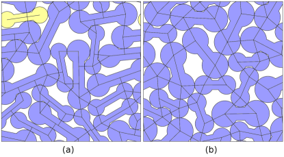
Figure 4: (a) A hypostatic and (b) an isostatic packing of $18$ dumbbells, with packing fractions $\phi=0.769$ and $0.806$, respectively. In (a) and (b), the shaft half-width is equal to half of the radius of the end disks. In (a) the length of the shaft is $4$ times the disk radius, whereas in (b), the shaft length is $2.4$ times the disk radius. In (a), the yellow particle has one unconstrained degree of freedom. Thus, if the particles formed an isostatic contact network, $N_{c}=3N-2=52$. The packing is hypostatic with $N_{c}=51$. In (b), the packing has no particles with unconstrained degrees of freedom. This packing is isostatic with $N_{c}=3N-1=53$.

The importance of specifying “accessible contact surface” in criterion (ii) can be demonstrated by the two packings of dumbbells in Fig. 4. In both cases, the particles are allowed to rotate, so criterion (i) is satisfied. The packing in (a) also satisfies criterion (ii) because the shaft is part of the accessible contact surface of the constituent particles, and the shaft cannot be defined as a finite union of disks. Thus, we expect hypostatic packings for the dumbbells in Fig. 4 (a). In contrast, in Fig. 4 (b), the shaft is not part of the accessible contact surface, because it is too short to allow the end disks of other particles to come into contact with it. Thus, the particles in Fig. 4 (b) do not satisfy criterion (ii), because the accessible contact surface is a union of two disks. We expect packings generated using the dumbbells in Fig. 4 (b) to be isostatic.

III.2 Packing Fraction, Coordination Number, and Eigenvalues of the Dynamical Matrix

In this section, we describe studies of the packing fraction and coordination number of packings of nonspherical particles at jamming onset as a function of the particle asphericity ${\cal A}$. We also calculate the eigenvalues of the dynamical matrix for packings of circulo-lines and circulo-polygons and show the eigenvalue spectrum as a function of decreasing pressure. We find that hypostatic packings possess a band of eigenvalues, i.e. the ‘quartic modes’, for which the energy increases as the fourth power in amplitude when we perturb the system along their eigendirections. These quartic modes are not observed in isostatic packings. We further show that the fourth derivative of the total potential energy in the direction of these quartic modes does not vanish at zero pressure, proving that packings possessing quartic modes are mechanically stable, despite being hypostatic.

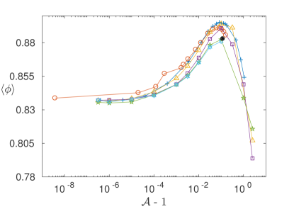
Figure 5: Packing fraction at jamming onset $\langle\phi\rangle$ (averaged over $50$ packings with random initial conditions) plotted versus asphericity ${\cal A}$ for a variety of nonspherical shapes: ellipses (circles), circulo-lines (plus signs), circulo-triangles (triangles), circulo-pentagons (squares), circulo-octagons (five-pointed stars), circulo-decagons (six-pointed stars), and Reuleaux triangles (filled black circle). The packings include $N=100$ particles, except for the ellipse packings, which contain $N=480$ particles.

In Fig. 5, we plot the average packing fraction at jamming onset versus ${\cal A}$ for all of the nonspherical particles we considered. The data for $\langle\phi\rangle$ nearly collapses onto a master curve, which tends to $\langle\phi\rangle\approx 0.84$ for small ${\cal A}-1$, as found for packings of bidisperse disks Xu et al. (2005), forms a peak near ${\cal A}-1\approx 10^{-1}$, and decreases strongly for ${\cal A}-1>10^{-1}$. This result suggests that the asphericity can serve as common descriptor of the structural and mechanical properties of packings of nonspherical particles, i.e. jammed packings with similar ${\cal A}$ will possess similar properties.

In Fig. 6, we plot the average coordination number

$$\langle z\rangle=\frac{2(N_{c}+1)}{N-N_{r}-N_{s}/3},$$ (3)

where $N_{c}$ is the number of contacts in the packing. The $+1$ in the factor of $N_{c}+1$ is included to account for the $-1$ in the expression for the number of contacts $N_{c}=N_{c}^{0}=3N-1$ in isostatic packings of nonspherical particles in 2D, where $N_{c}^{0}$ is the isostatic number of contacts. $N_{r}$ is the number of rattler particles that have unconstrained translational and rotational degrees of freedom. $N_{s}$ is the number of ‘slider’ particles with a single unconstrained translational degree of freedom. An example of a slider particle is the yellow particle in the packing of circulo-lines in Fig. 3 (c), which can translate along its long axis without energy cost. Defining the coordination number as in Eq. 3 ensures that an isostatic packing of circulo-lines, circulo-polygons, or other nonspherical particles will have $\langle z\rangle=6$. If $\langle z\rangle<6$, the packing is hypostatic.

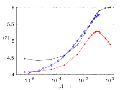
Figure 6: Coordination number $\langle z\rangle$ (defined in Eq. 3) as a function of asphericity ${\cal A}-1$ for ellipses (circles) and circulo-lines, counting a contact between nearly parallel circulo-lines as one contact (asterisks) or two contacts (plus signs).

In Fig. 6, we show the coordination number $\langle z\rangle$ in Eq. 3 versus ${\cal A}-1$ for packings of ellipses and circulo-lines for two ways of defining a contact between two nearly parallel circulo-lines. At low asphericities, where the particle shape approaches a disk, a nearly parallel contact is only able to apply a small torque to the two contacting particles, making it unlikely to constrain a rotational degree of freedom in addition to a translational degree of freedom. Thus, at low asphericities, nearly parallel contacts should only be counted as a single constraint. In Fig. 6, we show that $\langle z\rangle$ for ellipses and circulo-lines (counting nearly parallel contacts once) both approach $4$ in the limit ${\cal A}-1$ tends to zero.

In contrast, at large asphericities, nearly parallel contacts between two circulo-lines prevent the particles from rotating and translating (in a direction perpendicular to their shafts). Thus, for large ${\cal A}-1$, nearly parallel contacts should be counted as two constraints. In Fig. 6, we show that the coordination number $\langle z\rangle$ for packings of circulo-lines approaches $6$ in the large ${\cal A}-1$ limit when nearly parallel contacts are counted twice. These results suggest that we must interpolate between counting parallel contacts once at low asphericities, and counting them twice as the asphericity increases.

One way to resolve the question of whether to count a nearly parallel contact between nonspherical particles as one or two constraints is to calculate the dynamical matrix (all second derivatives of the total potential energy with respect to the particle coordinates) of the static packings, and examine the spectrum of the dynamical matrix eigenvalues, which in the harmonic approximation give the vibrational frequencies of the packing Tanguy et al. (2002). For details on the calculation of the entries of the dynamical matrix for circulo-lines and -polygons, see Appendix C.

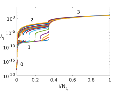
Figure 7: The eigenvalues $\lambda_{i}$ of the dynamical matrix sorted from smallest to largest for static packings of $N=100$ circulo-lines at the $17$ different asphericities ${\cal A}-1$ shown in Fig. 6 ranging from $\approx 10^{-6}$ to $1$ and decreasing from top to bottom. $N_{\lambda}=15000$ is the total number of eigenvalues in all of the packings at a given asphericity. For each asphericity (different colors), we show spectra for $50$ separate packings. We label four distinct regions of the eigenvalue spectra, $0$-$3$. Region $0$ ($\lambda_{i}\lesssim 10^{-14}$) corresponds to unconstrained degrees of freedom (such as overall translations due to periodic boundary conditions, rattler and slider particles), region $1$ ($10^{-14}\lesssim\lambda_{i}\lesssim 4\times 10^{-8}$) corresponds to “quartic modes,” whose number is determined by the number of missing contacts relative to the isostatic contact number, region $2$ corresponds to eigenmodes with predominantly rotational motion, and region $3$ corresponds to eigenmodes with predominantly translational motion.

In Fig. 7, we show the eigenvalue spectrum (sorted from smallest to largest) for static packings of circulo-lines over a wide range of aspect ratios ${\cal A}-1$ from $\approx 10^{-6}$ to $1$ (decreasing from top to bottom). As found in Ref. Mailman et al. (2009) for ellipse packings, the eigenvalue spectra for packings of circulo-lines possess several distinct regions. Region $0$ ($\lambda_{i}\lesssim 10^{-14}$, which is set by numerical precision) corresponds to unconstrained degrees of freedom, such as overall translations from periodic boundary conditions, and rattler and slider particles. Region $1$ ($10^{-14}\lesssim\lambda_{i}\lesssim 4\times 10^{-8}$) corresponds to “quartic modes,” whose number is determined by the number of missing contacts relative to the isostatic contact number. For the asphericities we consider, regions $2$ and $3$ correspond to eigenmodes with predominantly rotational and translational motion, respectively.

If we focus on all but the three smallest asphericities (i.e. the three rightmost curves in Fig. 7), we can define a cutoff value $\lambda_{c}$ that clearly separates regions $1$ and $2$. For packings of $N=100$ circulo-lines at pressure $P_{0}=10^{-9}$, $\lambda_{c}\approx 4\times 10^{-8}$. For asphericities where $\lambda_{c}$ distinguishes regions $1$ and $2$, the number of contacts in packings of circulo-lines satisfies $N_{c}=N^{0}_{c}-N_{1}$, where $N_{1}$ is the number of eigenvalues in region $1$. A key observation is that defining the number of contacts in this way for intermediate and high asphericities is the same as if $N_{c}$ is determined by the number of particle contacts, with nearly parallel contacts counted twice. For asphericities where the difference between regions $1$ and $2$ is more ambiguous, we still use $\lambda_{c}$ to determine whether a given eigenvalue belongs to region $1$ or $2$. For the lowest asphericities, we find that defining $N_{c}=N^{0}_{c}-N_{1}$ corresponds to counting one constraint for each nearly parallel contact.

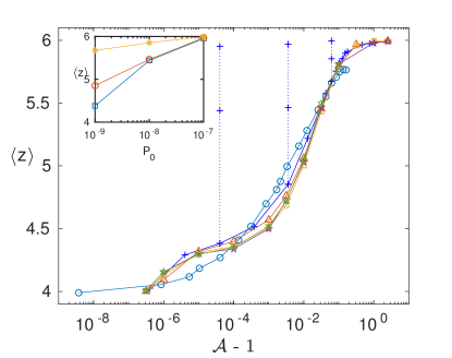
Figure 8: The average coordination number $\langle z\rangle$ (Eq. 3) is plotted versus asphericity ${\cal A}-1$ for packings of $N=100$ circulo-lines (plus signs), -triangles (triangles), -pentagons (squares), -octagons (five-pointed stars), and -decagons (six-pointed stars). This data is compared to $\langle z\rangle$ for packings of $N=480$ ellipses (circles). For packings of circulo-lines and -polygons, we define $\langle z\rangle$ using $N_{c}=N^{0}_{c}-N_{1}$. In the inset, we show $\langle z\rangle$ as a function of pressure $P_{0}$ for packings of circulo-lines for ${\cal A}-1=4\times 10^{-5}$ (squares), $3.6\times 10^{-3}$ (circles), and $6.2\times 10^{-2}$ (asterisks). $\langle z\rangle$ decreases more rapidly with $P$ at lower asphericities. All data points in the inset are also plotted in the main figure (plus signs connected by dotted lines).

In Fig. 8, we plot the average coordination number $\langle z\rangle$ from Eq. 3 using $N_{c}=N^{0}_{c}-N_{1}$ versus ${\cal A}-1$ for $N=100$ packings of circulo-lines and circulo-polygons. At low asphericities ${\cal A}-1$, the coordination number for packings of circulo-lines and circulo-polygons, as well as ellipses, approaches $\langle z\rangle=4$, which is expected for bidisperse disk packings. At large asphericities, $\langle z\rangle=6$ for packings of circulo-lines and circulo-polygons as expected for isostatic packings with $2$ translational and $1$ rotational degree of freedom per particle. $\langle z\rangle$ for ellipse packings plateaus for large ${\cal A}-1$. However, the current data suggests that the plateau value is less than $6$, indicating that ellipse packings are hypostatic for all ${\cal A}-1$.

An interesting feature in $\langle z\rangle({\cal A})$ for static packings of circulo-lines and -polygons is the plateau in $\langle z\rangle$ that occurs near ${\cal A}-1\approx 10^{-5}$ in Fig. 8. Our results suggest that the plateau is likely an artifact of the small, but nonzero pressure of the static packings. If the particles are overcompressed, even slightly, nearly parallel contacts will be able to exert larger torques than they would at zero pressure, which causes more eigenvalues to be above the eigenvalue threshold $\lambda_{c}$, and contacts to be counted as two constraints instead of one. Thus, as we decrease the pressure to zero, we expect to count fewer of these nearly parallel contacts as two constraints and the plateau in $\langle z\rangle$ near ${\cal A}-1\approx 10^{-5}$ will decrease. As ${\cal A}-1$ decreases below $10^{-5}$, the effects from overcompression are less important, and the nearly parallel contacts are only counted once.

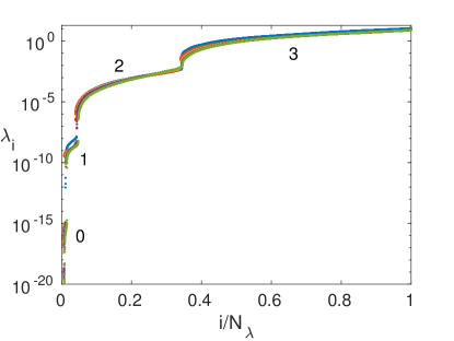
Figure 9: The eigenvalues $i$ of the dynamical matrix sorted from smallest to largest for static packings of $N=100$ circulo-lines (blue), -triangles (red), -pentagons (yellow), -octagons (purple), and -decagons (green) at asphericity ${\cal A}=1.1$. $N_{\lambda}=15000$ is the total number of eigenvalues in all of the packings of a given shape. For each particle shape, we show spectra for $50$ separate packings. Regions $0$-$3$ are defined the same way as in Fig. 7.

In Fig. 9, we plot the eigenvalues $\lambda_{i}$ sorted from smallest to largest for static packings of five different particle shapes (circulo-lines, -triangles, -pentagons, -octagons, and decagons) at the same asphericity, ${\cal A}=1.1$. We find that the eigenvalue spectra for all of these shapes are nearly identical. This behavior differs markedly from that in Fig. 7, where we show the eigenvalue spectra for packings with the same particle shape (circulo-lines), but at different values of the asphericity. Circulo-polygons with $n$ sides possess $2n-3$ parameters that specify their shape (not counting uniform scaling of lengths). Our results suggest that asphericity is a key parameter in determining the structure, geometry, and physical properties of hypostatic packings.

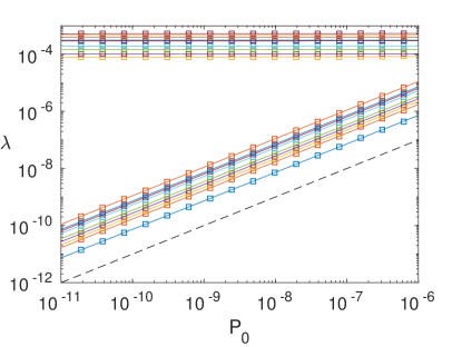
Figure 10: Nine eigenvalues $\lambda$ of the dynamical matrix from regions $1$ (bottom) and $2$ (top) plotted versus pressure $P_{0}$ for a static packing of $N=32$ circulo-lines with asphericity ${\cal A}=1.03$. The dashed line has slope $1$.

The reason why the eigenvalues in region $1$ (c.f. Fig. 7) are referred to as “quartic modes” is that, for perturbations along the corresponding eigenvectors, the total potential energy scales quartically with the amplitude of the perturbation, rather than quadratically, as one would expect for mechanically stable packings Mailman et al. (2009); Schreck et al. (2012). In Fig. 10, we plot eigenvalues from regions $1$ and $2$ as a function of pressure $P_{0}$ for a static packing of $N=32$ circulo-lines at asphericity ${\cal A}=1.03$. The eigenvalues from region $2$ are independent of pressure, whereas the eigenvalues from region $1$ scale linearly with pressure. Thus, for packings of circulo-lines and other particle shapes that yield hypostatic packings, the eigenvalues corresponding to the quartic modes are zero at jamming onset ($P_{0}=0$). This result agrees with prior studies of hypostatic packings of ellipses and ellipsoids Schreck et al. (2012).

Perturbations along the quartic modes are constrained to fourth order. In Fig. 11, we show the fourth derivatives of the total potential energy $d^{4}U/d{{\vec{\lambda}}}^{4}$ in the directions of the nine eigenmodes in region $1$ (that are depicted near the bottom of Fig. 10). We find that the fourth derivatives along eigenmodes in region $1$ do not depend on pressure, and thus remain nonzero at zero pressure. These findings demonstrate that hypostatic packings are fully constrained at zero pressure—in some directions by quadratic potentials and in other directions by quartic potentials.

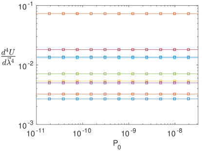
Figure 11: For the same packing as in Fig. 10, we plot the fourth derivative of the total potential energy $d^{4}U/d{\vec{\lambda}}^{4}$ in the direction of the nine eigenmodes in region $1$ in the bottom of Fig. 10 as a function of pressure $P_{0}$. All of the fourth derivatives for the region $1$ eigenmodes are independent of pressure.

III.3 Convex versus concave constraints

Why are hypostatic packings of circulo-lines and other nonspherical particles mechanically stable when they possess fewer contacts than the isostatic number, $N_{c}<N_{c}^{0}$? We have already shown that the number of missing contacts $N_{c}^{0}-N_{c}$ matches the number of quartic modes along which the energy increases quartically, not quadratically, with the perturbation amplitude. In the other $N_{c}$ eigendirections of the dynamical matrix, the energy increases quadratically with the perturbation amplitude. As a result, there are no directions in configuration space for which these hypostatic packings can be perturbed without energy cost, and thus they are mechanically stable.

To more fully address the question of how hypostatic packings of nonspherical particles can be mechanically stable, we consider the so-called “feasible region” of configuration space near each static packing for packing fractions slightly below jamming onset Donev et al. (2007). The feasible region near a given static packing includes all configurations for which there are no particle overlaps. The boundaries of this region are determined by all of the interparticle contacts, each of which corresponds to an inequality among the particle coordinates specifying when pairs of particles do not overlap. Points in configuration space that satisfy all of the inequalities are inside the feasible region. For mechanically stable packings, as the packing fraction is increased, the feasible region shrinks and becomes bounded and compact, preventing particle rearrangements that would allow the system to transition to a different packing. A static packing is mechanically stable if the feasible region of accessible configurations shrinks to a single point at jamming onset.

The number of constraints required to bound the feasible region depends on the curvature of the inequality constraints in configuration space, i.e. whether the constraints are concave or convex Donev et al. (2007). The inequality constraints that arise in disk packings are always concave. In particular, in disk packings, the curvature of each constraint is equal to minus the reciprocal of the sum of the radii of the two disks in contact. As a result, the number of contacts required to bound the feasible region for a mechanically stable packing of $N$ disks is $2N+1$ (minus $2$ from overall translations in periodic boundary conditions). Thus, hypostatic packings of nonspherical particles must possess contacts that give rise to bounding surfaces with convex curvature, which allows packings to be mechanically stable with fewer than the isostatic number of contacts.

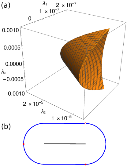
Figure 12: (a) Depiction of the feasible region of configurations that do not possess interparticle overlaps for a single circulo-line surrounded by three fixed points as shown in panel (b). This system is generated by fixing three points in space, initializing a circulo-line between the three points, and growing the interior circulo-line until it reaches force and torque balance while in contact with the three points. After finding the stable configuration, we decrease the diameter of the interior circulo-line by $10^{-7}$. The extent of the feasible region is shown using coordinates along the the three eigendirections (${\vec{\lambda}}_{1}$, ${\vec{\lambda}}_{2}$, and ${\vec{\lambda}}_{3}$) of the dynamical matrix for the interior circulo-line. The top contact (open circle) in (b), which is positioned along the shaft of the circulo-line, provides the constraint with convex curvature.

In Fig. 12, we show a simple configuration involving a circulo-line that gives rise to a convex constraint. We consider three points at fixed positions. These points represent less strict constraints than contacts with other circulo-lines, and thus, if these three points can constrain a circulo-line, three contacting circulo-lines will constrain an interior circulo-line as well. We initialize a circulo-line at several locations between the three points, and then increase the size of the interior circulo-line until it is constrained by the three points. After the circulo-line is constrained, we shrink its diameter by $10^{-7}$ so that it no longer overlaps the bounding points. The feasible region of the slightly undercompressed circulo-line is shown in Fig. 12 (a).

For an isostatic system, four contacts are required to constrain a circulo-line. However, we find configurations in which a circulo-line is constrained by only three contacts. Fig. 12 (a) illustrates the reason that only three contacts are necessary: one of the contacts (open circle on the top shaft) gives rise to a constraint with convex curvature in configuration space. In contrast, the other two contacts (filled circles), which are on the end caps of the circulo-line, give rise to constraints with concave curvature. This example suggests that only certain types of contacts between circulo-lines generate constraints with convex curvature, and thus the number of contacts required for mechanical stability is less than the isostatic number when these types of contacts are present.

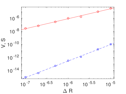
Figure 13: The volume $V$ (squares) and surface area $S$ (circles) of the feasible region in Fig. 12 (a) plotted as a function of the decrease in radius $\Delta R=R_{j}-R$, where $R_{j}$ is the radius at which the system is fully constrained. The solid and dashed lines have slopes $2.5$ and $1.5$, respectively.

To verify that the circulo-line “packing” in Fig. 12 (b) is mechanically stable, we numerically calculated the volume $V$ and surface area $S$ of the feasible region as a function of the degree of undercompression, $\Delta R=R_{j}-R$, where $R_{j}$ is the radius of the interior circulo-line at which the system is jammed. In Fig. 13, we show that both $V$ and $S$ display power-law scaling with $\Delta R$, emphasizing that the feasible region for hypostatic packings shrinks to a point, and thus these packings are mechanically stable.

Table 2: The principal curvatures ($\langle\kappa_{1}\rangle$ and $\langle\kappa_{2}\rangle$) for the different types of contacts that can occur between two circulo-lines in a $N=24$ packing of bidisperse circulo-lines with asphericity ${\cal A}=1.04$, averaged over all contacts in the packing of that type. Note that for $\kappa_{2}$ for an end particle in a parallel contact, the magnitude of the curvature was averaged, rather than the signed curvature, because, unlike any of the other curvatures, this one fluctuated between positive and negative. This type of averaging is denoted using the $\pm$ symbol.

Contact Type	$\langle\kappa_{1}\rangle$	$\langle\kappa_{2}\rangle$
Parallel (End Particle)	$0$	$(\pm)7.93\times 10^{-9}$
Parallel (Middle Particle)	$-1.29$	$0.774$
End-Middle (End Particle)	$-0.0261$	$0$
End-Middle (Middle Particle)	$-1.29$	$0.774$
End-End	$-5.69$	$-0.0246$

To further investigate the effect of convex and concave constraints on a hypostatic jammed packing, we measured the curvatures of the inequality constraints for each contact in a static packing with $N=24$ bidisperse circulo-lines with asphericity ${\cal A}=1.04$. We classified the contacts into five types as defined in Appendix A. Parallel contacts can involve the shaft of one circulo-line (middle) and the end cap of another (end). This arrangement gives rise to two types of contacts, one for the circulo-line with a contact on its end and another for the circulo-line with a contact on its middle. Similarly, the shaft (middle) of one circulo-line can be in contact with the end cap (end) of another, but the long axes are not parallel. This arrangement again gives rise to two types of contacts, one for the circulo-line with a contact on its end and another for the circulo-line with a contact on its middle. In addition, the ends of two circulo-lines can be in contact.

The average curvatures of the bounding surfaces for each contact type in a static packing of $N=24$ bidisperse circulo-lines are compiled in Table 2. (We find similar average values for other $N=24$ packings of bidisperse circulo-lines.) From this data, we can draw several conclusions about the contribution of each type of contact to the stability of circulo-line packings. First, end-end contacts yield concave constraints in configuration space, and thus on their own do not give rise to mechanically stable hypostatic packings. In contrast, end-middle contacts have a positive principal curvature for the circulo-line whose middle is in contact, and thus serve to stabilize hypostatic packings. Parallel contacts also possess a positive curvature associated with the circulo-line whose middle is in contact. However, note that the concave curvature for circulo-lines whose end is in parallel contact is much smaller than the concave curvature of the end circulo-line for end-middle contacts. This means that for circulo-lines with end contacts, the parallel contacts are more “stabilizing” than the end-middle contacts, and therefore they are more frequent in mechanically stable hypostatic circulo-line packings than other end-middle contacts.

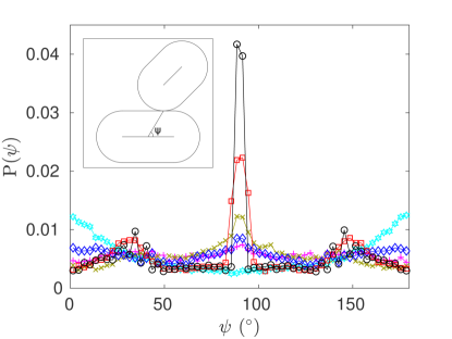
Figure 14: Probability distribution $P(\psi)$ of the contact angles $\psi$ in bidisperse ellipse ($N=480$) and circulo-line ($N=100$) packings at several asphericities: ellipses at ${\cal A}-1=0.19$ (six-pointed stars), $5\times 10^{-3}$ (plus signs), and $4\times 10^{-5}$ (exes), and circulo-lines at ${\cal A}-1=0.18$ (diamonds), $4\times 10^{-3}$ (squares), and $4\times 10^{-5}$ (circles). In the inset, we define the contact angle $\psi$ as the angle between the shaft of a circulo-line and the vector pointing from its center to the point of contact with another circulo-line. We use a similar definition for the contact angle for ellipses. Packings of circulo-lines, as well ellipses, favor parallel contacts, even at small asphericities.

The above observations about the curvatures of the inequality constraints in configuration space can help explain the distribution of contact angles $P(\psi)$ in static packings of elongated particles Tian et al. (2015); Marschall and Teitel shown in Fig. 14. This figure shows that, even for packings of circulo-lines at very small asphericities, parallel contacts are highly probable, despite the fact that the range of angles for parallel contacts at low asphericities is small. This behavior for $P(\psi)$ can be explained by the fact that end-middle and parallel contacts can contribute to making a hypostatic packing mechanically stable, whereas end-end contacts cannot. (See Table 2.) Thus, end-middle and parallel contacts (whose contact angles are close to $90^{\circ}$ at low asphericities) must be present to stabilize hypostatic packings of low-asphericity circulo-lines. As shown in Fig. 14, $P(\psi)$ is similar for both ellipse and circulo-line packings.

IV Conclusions and Future Directions

In this article, we carried out computational studies of static packings of frictionless nonspherical particles in 2D. We developed an interparticle potential for circulo-lines and -polygons that generates continuous pair forces and torques as a function of the particle coordinates. As a result, we are able to compare the structural and mechanical properties of mechanically stable packings of nine different nonspherical particle shapes: circulo-lines, -triangles, -pentagons, -octagons, -decagons, asymmetric dimers, dumbbells, Reuleaux triangles, and ellipses. Our studies place a particular emphasis on the question of which particle shapes give rise to hypostatic mechanically stable packings with fewer contacts than the isostatic number.

We conjecture that to form hypostatic mechanically stable packings, frictionless, convex particles must satisfy the following two criteria: (i) the particle has one or more nontrivial rotational degrees of freedom, and (ii) the particle cannot be defined as a union of a finite number of complete disks without changing its accessible contact surface. If the particle does not satisfy both criteria, we expect it to form isostatic packings. Packings of the nine particle shapes we considered are consistent with this conjecture. Future research can investigate methods to analytically prove this conjecture Roux (2000).

We then studied the packing fraction $\phi$ and coordination number $z$ at jamming onset for packings of a number of different types of nonspherical shapes in 2D as a function of asphericity ${\cal A}$. To do this, we resolved the ambiguity in the constraint counting of nearly parallel contacts of circulo-lines and -polygons using the branched structure of the eigenvalue spectra of the dynamical matrix. In future research, we will study the coordination number of packings of sphero-cylinders and -polygons in 3D, and compare the results to those in 2D, since it is extremely unlikely for sphero-cylinders and -polygons to form nearly parallel contacts.

We find that the packing fraction and coordination number obey approximate master curves when plotted versus the asphericity. Further, the eigenvalue spectra for different particle shapes, at the same ${\cal A}$, collapse. These results suggest that asphericity is a key parameter in determining the structure, geometry, and mechanical properties of hypostatic packings. For $n$-sided circulo-polygons, there are $2n-3$ parameters that specify their shape. In future studies, we will investigate additional shape parameters, such as the ratios of the area moments and others Schröder-Turk et al. (2013), to better understand the coupling between the shape parameter space and the properties of hypostatic packings of nonspherical particles.

We also demonstrated that hypostatic packings of circulo-lines (and by analogy circulo-polygons) are mechanically stable by showing that even though the eigenvalues of the dynamical matrix for the quartic modes tend to zero at zero pressure, the fourth derivatives of the total potential energy in the directions of the quartic modes do not. Thus, hypostatic packings of nonspherical particles are stable to perturbations in all directions in configuration space. Perturbations in some directions give rise to quadratic potentials, whereas other directions give rise to quartic potentials. In the directions with quartic potentials, we expect large anharmonic contributions to the vibrational and mechanical response Schreck et al. (2014).

In addition, we measured the curvatures of the inequality constraints that arise from interparticle contacts in hypostatic packings of circulo-lines to better understand the grain-scale mechanisms that allow hypostatic packings to be mechanically stable. The contacts in isostatic disk packings give rise to inequality constraints with only concave (negative) curvatures. In contrast, hypostatic packings of circulo-lines (and other nonspherical particles) possess different types of contacts (e.g. end-end and end-middle). Some types yield inequality constraints with concave curvatures and others yield inequality constraints with convex curvatures. We find that contacts with convex inequality constraints are present even at small asphericities. The contacts with convex inequality constraints allow the feasible region of slightly undercompressed hypostatic packings to be compact, bounded, and shrink to zero in the limit that the free volume tends to zero.

Appendix A Continuous Potential between Circulo-lines and -Polygons

The repulsive potential between two circulo-lines is given by Eq. (1), where $r_{ij}$ is the magnitude of ${\vec{r}}_{ij}$, which points from the location where the force is applied on circulo-line $j$ to the location where the force is applied on circulo-line $i$. These points of contact can be located on the ends or the shaft (middle) of a circulo-line. In this Appendix, we define the overlap distance $\delta=\sigma_{ij}-r_{ij}$, which will depend on the type of contact that occurs between two circulo-lines.

A.1 Types of Contacts

There are three types of interparticle contacts that occur in packings of circulo-lines: 1) the end of one circulo-line is in contact with the middle of another (Fig. 15), 2) the shafts of two circulo-lines are in contact and the circulo-lines are nearly parallel (Figs. 16 and 17), and 3) the ends of two circulo-lines are in contact (Fig. 18). Below, we define the overlap distance $\delta$ in the circulo-line potential (Eq. 1) for each type of contact.

A.1.1 End-middle Contacts

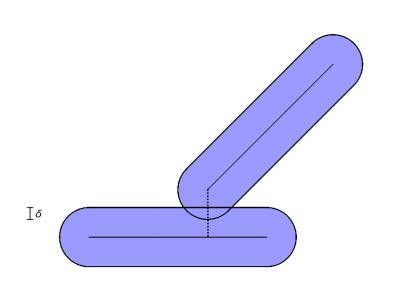
Figure 15: A contact between the endcap of one circulo-line and the middle of another. The separation between the circulo-lines $r_{ij}$ is indicated by the dotted line between the circulo-line shafts. The separation vector ${\vec{r}}_{ij}$ connects the end of the shaft of one circulo-line to the shaft of the other and is perpendicular to shaft of the circulo-line with the middle contact. The overlap is defined as $\delta=\sigma_{ij}-r_{ij}$, where $\sigma_{ij}$ is the sum of the endcap radius and the half-width of the shaft it overlaps.

End-middle contacts occur when the endcap of one circulo-line makes contact with the middle of another circulo-line, but does not overlap with either of the other circulo-line’s endcaps. (See Fig. 15.) In this case, we assume that the separation vector ${\vec{r}}_{ij}$ between circulo-lines points from the end of the shaft of the circulo-line with the end contact to the shaft of the other circulo-line. ${\vec{r}}_{ij}$ is perpendicular to the shaft of the circulo-line with the middle contact. The overlap between circulo-lines with an end-middle contact is $\delta=\sigma_{ij}-r_{ij}$, as shown in Fig. 15.

A.1.2 Parallel and Nearly Parallel Contacts

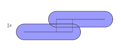
Figure 16: When two circulo-lines possess a parallel contact, it is counted twice, as two end-middle contacts. The separations $r_{ij}$ are depicted by the vertical dotted lines between the circulo-line shafts, and ${\vec{r}}_{ij}$ points from the end of one of the shafts to the other and is perpendicular to the shafts. The overlap is given by $\delta=\sigma_{ij}-r_{ij}$ for both contacts, where $\sigma_{ij}$ is the sum of the endcap radius and the half-width of the shaft it overlaps.

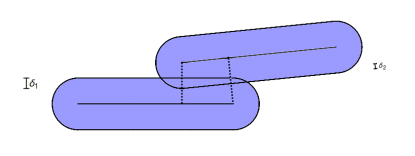
Figure 17: When the shafts of two contacting circulo-lines are close to parallel, such that both endcaps overlap the shaft of the other circulo-line, the contact is counted twice as for parallel contacts. Each separation vector ${\vec{r}}_{ij}$ (depicted by dotted lines between circulo-line shafts) points from the end of the shaft of the circulo-line with an end contact to the shaft of the circulo-line with the middle contact, and is perpendicular to the shaft of the circulo-line with the middle contact. The overlaps are given by $\delta_{1,2}=\sigma_{ij}-r_{ij}$ for the two contacts with different separations, where $\sigma_{ij}$ is the sum of the endcap radius and the half-width of the shaft it overlaps.

For parallel and nearly parallel contacts, an endcap of both circulo-lines overlaps the shaft of the other circulo-line. In this case, the spring potential in Eq. 1 for both overlaps is calculated as for end-middle contacts. If the circulo-lines are parallel, as in Fig. 16, $\delta=\sigma_{ij}-r_{ij}$ is the same for both overlaps. However, for nearly parallel contacts, as in Fig. 17, the separations are different for the two end-middle overlaps. This method for treating end-middle, parallel, and nearly parallel contacts ensures continuity of the potential as a function of the particle coordinates. If the circulo-lines in Fig. 17 rotate until their orientations match Fig. 15, the potential, force, and torque must all change continuously. Using our method, $\delta_{2}$ decreases continuously to zero as the contact evolves from that in Fig. 17 to that in Fig. 15. In addition, $\delta_{1}$ decreases continuously to zero as the circulo-lines in Fig. 17 rotate until $\delta_{2}$ is the only overlap.

A.1.3 End-End Contact

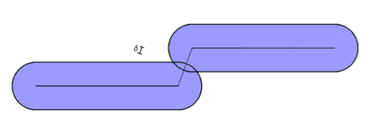
Figure 18: An end-end contact between the endcaps of two circulo-lines. The separation ${\vec{r}}_{ij}$ between circulo-lines (dotted line) gives the distances between the ends of the shafts of the two circulo-lines. The overlap is given by $\delta=\sigma_{ij}-r_{ij}$, where $\sigma_{ij}$ is the sum of the radii of the endcaps.

Also, suppose that we slide the two circulo-lines in Fig. 16 away from each other until they are similar to the configuration in Fig. 18 and form an end-end contact. In this case, we assume that the two overlap potentials add together as soon as the two relevant ends of the circulo-line shafts slide past each other. Therefore, to ensure continuity, the interaction potential for an end-end contact must be twice as large as that for an end-middle contact. Hence, we use $U=k\delta^{2}$ for end-end contacts.

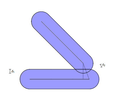
Figure 19: When a contact between circulo-lines is close to the boundary between the end of one and middle of another circulo-line, we include both the end-end and end-middle overlaps to ensure continuity as the contact crosses the boundary. The separation vector ${\vec{r}}_{ij}$ associated with the end-middle overlap, $\delta_{1}$ (vertical dotted line), points from the end of the shaft of one circulo-line to the shaft of the other, such that it is perpendicular to the shaft. The separation vector associated with the end-end overlap, $\delta_{2}$ (diagonal dotted line), points from the end of the shaft of one of the circulo-lines to the end of the shaft of the other overlapping circulo-line.

However, this treatment of end-end contacts creates a discontinuity for the configuration in Fig. 19. If we imagine sliding the circulo-lines past each other until the overlap $\delta_{1}$ is associated with an end-end contact, the potential will suffer a discontinuous jump from $\tfrac{1}{2}k\delta_{1}^{2}$ to $k\delta_{1}^{2}$ since the end-end contact potential is twice as large as an end-middle potential. To remedy this discontinuity, we add the end-end contact potential between the two relevant endpoints as soon as they become close enough to overlap. However, we do not make the end-end potential twice as large in this case. Hence, the potential in this case is given by $U=\tfrac{1}{2}k\left(\delta_{1}^{2}+\delta_{2}^{2}\right)$. Thus, when we perform that same sliding transformation, the potential will grow continuously from $\tfrac{1}{2}k\delta_{1}^{2}$ to $k\delta_{1}^{2}$ as $\delta_{2}$ grows continuously from 0 to $\delta_{1}$. Note that we do not add this end-end overlap potential if two end-middle contacts are present, as in Fig. 20, because in that case, the potential will already change continuously as described in the previous subsection, and hence there is no discontinuity to remedy.

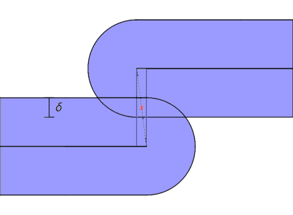
Figure 20: We do not calculate the end-end overlap potential for parallel and nearly parallel circulo-lines since this would lead to a discontinuity if the configuration transitions to an end-end contact by sliding. Instead, we choose the circulo-line separations for parallel and nearly parallel contacts as shown in Fig. 16. The separation associated with an end-end contact is indicated by the dashed line with an $x$ in the middle.

A.2 Generalizing the Circulo-line Potential to Circulo-Polygons

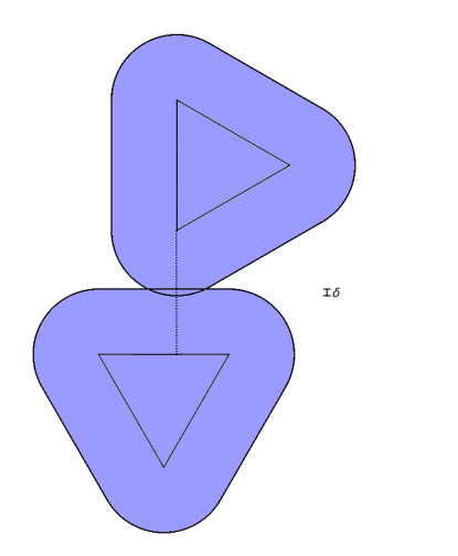
Figure 21: A schematic of an end-middle contact between two circulo-triangles. The separation $r_{ij}$ between circulo-triangles (dotted line) is given by the perpendicular distance between the vertex of the circulo-triangle with the end contact and the side of the closest side of the triangle in the circulo-triangle with the middle contact. The overlap $\delta=\sigma_{ij}-r_{ij}$, where $\sigma_{ij}$ is the sum of the endcap radius and half-width of the shaft it overlaps.

Generalizing our continuous circulo-line potential to circulo-polygons, such as those pictured in Fig. 21, is straightforward. We simply calculate the potential between all pairs of circulo-lines that comprise each circulo-polygon. For example, in Fig. 21, since the vertex of the top circulo-triangle is shared by two circulo-lines, we count the end-middle contact twice, and hence the overlap potential is $U=k\delta^{2}$.

Appendix B Generation of Circulo-Polygons

A circulo-polygon is formed through a Minkowski sum of a polygon and a disk with a radius $r$ Oks and Sharir (2006), which is equivalent to the sweeping of the disk around the profile of the polygon as in Fig. 22 (a). The shape of a circulo-polygon with $n$ edges is fully specified by $2n-3$ independent parameters. In this work, we focus on the asphericity shape parameter ${\cal A}$, which measures the deviation of a given shape from a circle in 2D.

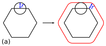
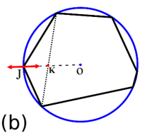
Figure 22: (a) A circulo-polygon is the Minkowski sum of a polygon (e.g. the regular hexagon on the left) and a disk with radius $r$, which is “swept” along the edges of the polygon to form the circulo-polygon (the red shape on right). (b) Schematic of the generation of a circulo-polygon at a given asphericity ${\cal A}$. First, we select $n$ random points on a unit circle (blue curve) with origin $O$ (where $n$ is the desired number of edges). We then randomly choose vertex $J$ and either stretch or shorten the distance between $J$ and $O$ (dashed line) by an amount randomly chosen between 0 and the distance $JK$ to adjust ${\cal A}$ to match the target asphericity.

We study bidisperse packings of circulo-polygons with asphericity ${\cal A}$ for which half of the circulo-polygons are large and half are small. The large circulo-polygons have areas that satisfy $a_{L}=1.4^{2}a_{S}$, where $a_{L,S}$ is the area of the large and small circulo-polygons, respectively. The large circulo-polygons (and small ones) have different shapes at the same ${\cal A}$. We generate different circulo-polygons at the same ${\cal A}$ using the following two-step approach: 1) We first randomly select $n$ points on a unit disk as the vertices of an $n$-sided polygon. The radius $r$ of the circulo-polygon is set to be $n$ percent of the perimeter of the polygon. 2) If the asphericity of the current circulo-polygon is smaller than the target $\cal A$, a vertex $J$ is randomly chosen and then stretched or shortened along the direction between the vertex $J$ and the center $O$ of the unit disk, by a distance randomly chosen between 0 and the distance between $J$ and the intersection of $JO$ with the line segment connecting the two neighboring vertices, as shown in Fig. 22 (b). This deformation is accepted only if the asphericity of the new shape is closer to $\cal A$ than the original and the new shape is still convex. If the asphericity of the current circulo-polygon exceeds ${\cal A}$, the radius $r$ is increased to match the target $\cal A$. We repeat step $2$ until a circulo-polygon with ${\cal A}$ is obtained.

Appendix C Dynamical Matrix Elements of Circulo-Polygon Packings

In this Appendix, we provide explicit expressions for the dynamical matrix elements for static packings of circulo-polygons that interact via the purely repulsive linear spring potential in Eq. 1. In this expression, $R_{i}$ is radius that forms the edge of circulo-polygon $i$ and ${\vec{r}}_{ji}$ is the separation vector from circulo-polygon $i$ to $j$, which is is given by

$$\vec{r}_{ji}=\vec{c}_{ji}+{\cal R}_{j}\vec{v}_{n}-{\cal R}_{i}\vec{v}_{m}+{\cal R}_{j}\hat{u}_{n}l_{n}-{\cal R}_{i}\hat{u}_{m}l_{m},$$ (4)

where $\vec{c}_{ji}=(x_{j}-x_{i},y_{j}-y_{i})\equiv(p,q)$ is the center-to-center separation between circulo-polygons, ${\cal R}_{i}=\left[\begin{array}[]{cccc}\cos\theta_{i}&-\sin\theta_{i}\\ \sin\theta_{i}&\cos\theta_{i}\end{array}\right]$ is the rotation matrix in 2D, $\theta_{i}$ is the orientation of particle $i$ relative to the $x$-axis, $\vec{v}_{m}$ is the vector from the center of particle $i$ to the center of its corresponding edge $m$ when particle $i$ at zero rotation, ${\hat{u}}_{m}$ is the unit vector along edge $m$ at zero rotation, and $l_{m}$ indicates the distance between the contact point and the center of edge $m$.

The dynamical matrix requires the calculation of the second derivatives of the total potential energy $U$, and can be expressed in terms of the first and second derivatives of the contact distance $r_{ji}$ with respect to the particle coordinates:

$$\frac{\partial^{2}U}{\partial\xi_{i}\partial\xi_{j}}=\frac{\partial{r_{ji}}}{\partial\xi_{i}}\frac{\partial{r_{ji}}}{\partial\xi_{j}}-\left(\sigma_{ji}-r_{ji}\right)\frac{\partial^{2}{r_{ji}}}{\partial\xi_{i}\partial\xi_{j}},$$ (5)

where $\xi_{i}=x_{i}$, $y_{i}$, or $\theta_{i}$,

$$\frac{\partial{r_{ji}}}{\partial\xi_{i}}=\frac{\vec{r}_{ji}}{r_{ji}}\cdot\frac{\partial\vec{r}_{ji}}{\partial\xi_{i}},$$ (6)

and

$$\frac{\partial^{2}{r_{ji}}}{\partial\xi_{i}\partial\xi_{j}}=\frac{1}{r_{ji}}\left(\frac{\partial\vec{r}_{ji}}{\partial\xi_{i}}\cdot\frac{\partial\vec{r}_{ji}}{\partial\xi_{j}}+\vec{r}_{ji}\cdot\frac{\partial^{2}\vec{r}_{ji}}{\partial\xi_{i}\partial\xi_{j}}-\frac{\partial{r_{ji}}}{\partial\xi_{i}}\frac{\partial{r_{ji}}}{\partial\xi_{j}}\right).$$ (7)

There are two types of contacts among circulo-polygons. The first type is a vertex-to-edge contact. Assuming the end point of edge $n$ on particle $j$ is in contact with edge $m$ on particle $i$, $l_{n}$ is half of the length of edge $n$, and $l_{m}$ can be written as

$$l_{m}=\left(\vec{c}_{ji}+{\cal R}_{j}\vec{v}_{n}-{\cal R}_{i}\vec{v}_{m}+{\cal R}_{j}\hat{u}_{n}l_{n}\right)\cdot{\cal R}_{i}\vec{u}_{m}.$$ (8)

In Eq. 8, $\vec{v}_{m}$, $\vec{v}_{n}$, $\hat{u}_{m}$, and $\hat{u}_{n}$ are defined as

$$\vec{v}_{m}=\left(m\cos a,m\sin a\right),$$ (9)

$$\vec{v}_{n}=\left(n\cos b,n\sin b\right),$$ (10)

$$\hat{u}_{m}=\left(\cos d,\sin d\right),$$ (11)

and

$$\hat{u}_{n}=\left(\cos e,\sin e\right),$$ (12)

where $m$ and $n$ are the magnitudes of $\vec{v}_{m}$ and $\vec{v}_{n}$, respectively, and the angles $a$, $b$, $d$, and $e$ are the orientations of $\vec{v}_{m}$, $\vec{v}_{n}$, $\hat{u}_{m}$, and $\hat{u}_{n}$, respectively. The contact distance $r_{ji}$ is

$$r_{ji}=|q\cos(d+\theta_{i})-m\sin(a-d)+n\sin\beta+\\ l_{n}\sin\Delta-p\sin(d+\theta_{i})|,$$ (13)

where

$$\beta=b-d+\theta_{j}-\theta_{i}$$ (14)

and

$$\Delta=e-d+\theta_{j}-\theta_{i}.$$ (15)

The nonzero first and second derivatives can be expressed as:

$$\frac{\partial{r_{ji}}}{\partial x_{i}}=\Xi\,\sin(d+\theta_{i}),$$ (16)

$$\frac{\partial{r_{ji}}}{\partial y_{i}}=-\Xi\,\cos(d+\theta_{i}),$$ (17)

$$\frac{\partial{r_{ji}}}{\partial\theta_{i}}=-\Xi\,\bigl{[}n\cos\beta+l_{n}\cos\Delta+\\ p\cos(d+\theta_{i})+q\sin(d+\theta_{i})\bigr{]},$$ (18)

$$\frac{\partial{r_{ji}}}{\partial x_{j}}=-\frac{\partial{r_{ji}}}{\partial x_{i}},$$ (19)

$$\frac{\partial{r_{ji}}}{\partial y_{j}}=-\frac{\partial{r_{ji}}}{\partial y_{i}},$$ (20)

$$\frac{\partial{r_{ji}}}{\partial\theta_{j}}=-\Xi\,\left[n\cos\beta+l_{n}\cos\Delta\right],$$ (21)

$$\frac{\partial^{2}{r_{ji}}}{\partial x_{i}\partial\theta_{i}}=-\frac{\partial{r_{ji}}}{\partial y_{i}},$$ (22)

$$\frac{\partial^{2}{r_{ji}}}{\partial y_{i}\partial\theta_{i}}=\frac{\partial{r_{ji}}}{\partial x_{i}},$$ (23)

$$\frac{\partial^{2}{r_{ji}}}{\partial\theta_{i}\partial\theta_{i}}=-\Xi\,\bigl{[}n\sin\beta+l_{n}\sin\Delta-\\ p\sin(d+\theta_{i})+q\cos(d+\theta_{i})\bigr{]},$$ (24)

$$\frac{\partial^{2}{r_{ji}}}{\partial x_{j}\partial\theta_{i}}=\frac{\partial{r_{ji}}}{\partial y_{i}},$$ (25)

$$\frac{\partial^{2}{r_{ji}}}{\partial y_{j}\partial\theta_{i}}=-\frac{\partial{r_{ji}}}{\partial x_{i}},$$ (26)

$$\frac{\partial^{2}{r_{ji}}}{\partial\theta_{j}\partial\theta_{i}}=\Xi\,\left[n\sin\beta+l_{n}\sin\Delta\right],$$ (27)

and

$$\frac{\partial^{2}{r_{ji}}}{\partial\theta_{j}\partial\theta_{j}}=-\frac{\partial^{2}{r_{ji}}}{\partial\theta_{j}\partial\theta_{i}}.$$ (28)

In the expressions in Eqs. 16-28, $\Xi$ is defined as:

$$\Xi=\textrm{Sgn}\bigl{(}q\cos(d+\theta_{i})-m\sin(a-d)+n\sin\beta+\\ l_{n}\sin\Delta-p\sin(d+\theta_{i})\bigr{)},$$ (29)

where

$$\textrm{Sgn}\left(z\right)=\begin{cases}1,\quad&z>0\\ 0,\quad&z=0\\ -1,\quad&z<0.\end{cases}$$ (30)

All of the other first and second derivatives are zero.

The second type of contact between circulo-polygons is a a contact between two vertices. In this case, $l_{m}$ and $l_{n}$ are each half the lengths of edges $m$ and $n$, respectively. The $x$- and $y$-components of separation vector $\vec{r}_{ji}$ are

$$x_{ji}=p+n\cos(b+\theta_{j})+l_{n}\cos(e+\theta_{j})-\\ m\cos(a+\theta_{i})-l_{m}\cos(d+\theta_{i})$$ (31)

and

$$y_{ji}=q+n\sin(b+\theta_{j})+l_{n}\sin(e+\theta_{j})-\\ m\sin(a+\theta_{i})-l_{m}\sin(d+\theta_{i}).$$ (32)

For vertex-vertex contacts, the nonzero first and second derivatives are:

$$\frac{\partial{r_{ji}}}{\partial x_{i}}=-\frac{x_{ji}}{r_{ji}},$$ (33)

$$\frac{\partial{r_{ji}}}{\partial y_{i}}=-\frac{y_{ji}}{r_{ji}},$$ (34)

$$\frac{\partial{r_{ji}}}{\partial\theta_{i}}=\frac{1}{r_{ji}}(-l_{m}\bigl{[}q\cos(d+\theta_{i})-p\sin(d+\theta_{i})+\\ n\sin\beta+l_{n}\sin\Delta\bigr{]}+m\bigl{[}p\sin(a+\theta_{i})-q\cos(a+\theta_{i})-\\ n\sin\omega+l_{n}\sin\mu\bigr{]}),$$ (35)

$$\frac{\partial{r_{ji}}}{\partial x_{j}}=-\frac{\partial{r_{ji}}}{\partial x_{i}},$$ (36)

$$\frac{\partial{r_{ji}}}{\partial y_{j}}=-\frac{\partial{r_{ji}}}{\partial y_{i}},$$ (37)

$$\frac{\partial{r_{ji}}}{\partial\theta_{j}}=\frac{1}{r_{ji}}(l_{n}\bigl{[}q\cos(e+\theta_{j})-p\sin(e+\theta_{j})-\\ m\sin\mu+l_{m}\sin\Delta\bigr{]}+n\bigl{[}q\cos(b+\theta_{j})-p\sin(b+\theta_{j})+\\ m\sin\omega+l_{m}\sin\beta\bigr{]}),$$ (38)

$$\frac{\partial\vec{r}_{ji}}{\partial x_{i}}\cdot\frac{\partial\vec{r}_{ji}}{\partial x_{i}}=\frac{\partial\vec{r}_{ji}}{\partial y_{i}}\cdot\frac{\partial\vec{r}_{ji}}{\partial y_{i}}=\frac{\partial\vec{r}_{ji}}{\partial x_{j}}\cdot\frac{\partial\vec{r}_{ji}}{\partial x_{j}}=\frac{\partial\vec{r}_{ji}}{\partial y_{j}}\cdot\frac{\partial\vec{r}_{ji}}{\partial y_{j}}=1,$$ (39)

$$\frac{\partial\vec{r}_{ji}}{\partial x_{i}}\cdot\frac{\partial\vec{r}_{ji}}{\partial x_{j}}=\frac{\partial\vec{r}_{ji}}{\partial y_{i}}\cdot\frac{\partial\vec{r}_{ji}}{\partial y_{j}}=-1,$$ (40)

$$\frac{\partial\vec{r}_{ji}}{\partial x_{i}}\cdot\frac{\partial\vec{r}_{ji}}{\partial\theta_{i}}=-m\sin(a+\theta_{i})-l_{m}\sin(d+\theta_{i}),$$ (41)

$$\frac{\partial\vec{r}_{ji}}{\partial x_{i}}\cdot\frac{\partial\vec{r}_{ji}}{\partial\theta_{j}}=n\sin(b+\theta_{i})+l_{n}\sin(e+\theta_{j}),$$ (42)

$$\frac{\partial\vec{r}_{ji}}{\partial y_{i}}\cdot\frac{\partial\vec{r}_{ji}}{\partial\theta_{i}}=m\cos(a+\theta_{i})+l_{m}\cos(d+\theta_{i}),$$ (43)

$$\\ \frac{\partial\vec{r}_{ji}}{\partial y_{i}}\cdot\frac{\partial\vec{r}_{ji}}{\partial\theta_{j}}=-n\cos(b+\theta_{i})-l_{n}\cos(e+\theta_{j}),$$ (44)

$$\frac{\partial\vec{r}_{ji}}{\partial\theta_{i}}\cdot\frac{\partial\vec{r}_{ji}}{\partial\theta_{i}}=l_{m}^{2}+m^{2}+2l_{m}m\cos(a-d),$$ (45)

$$\frac{\partial\vec{r}_{ji}}{\partial\theta_{i}}\cdot\frac{\partial\vec{r}_{ji}}{\partial x_{j}}=-\frac{\partial\vec{r}_{ji}}{\partial x_{i}}\cdot\frac{\partial\vec{r}_{ji}}{\partial\theta_{i}},$$ (46)

$$\frac{\partial\vec{r}_{ji}}{\partial\theta_{i}}\cdot\frac{\partial\vec{r}_{ji}}{\partial y_{j}}=-\frac{\partial\vec{r}_{ji}}{\partial y_{i}}\cdot\frac{\partial\vec{r}_{ji}}{\partial\theta_{i}},$$ (47)

$$\frac{\partial\vec{r}_{ji}}{\partial\theta_{i}}\cdot\frac{\partial\vec{r}_{ji}}{\partial\theta_{j}}=-n(l_{m}\cos\beta+m\cos\omega)-\\ l_{n}(l_{m}\cos\Delta+m\cos\mu),$$ (48)

$$\frac{\partial\vec{r}_{ji}}{\partial x_{j}}\cdot\frac{\partial\vec{r}_{ji}}{\partial\theta_{j}}=-\frac{\partial\vec{r}_{ji}}{\partial x_{i}}\cdot\frac{\partial\vec{r}_{ji}}{\partial\theta_{j}},$$ (49)

$$\frac{\partial\vec{r}_{ji}}{\partial y_{j}}\cdot\frac{\partial\vec{r}_{ji}}{\partial\theta_{j}}=-\frac{\partial\vec{r}_{ji}}{\partial y_{i}}\cdot\frac{\partial\vec{r}_{ji}}{\partial\theta_{j}},$$ (50)

$$\frac{\partial\vec{r}_{ji}}{\partial\theta_{j}}\cdot\frac{\partial\vec{r}_{ji}}{\partial\theta_{j}}=l_{n}^{2}+n^{2}+2l_{n}n\cos(b-e),$$ (51)

and

$$\vec{r}_{ji}\cdot\frac{\partial^{2}\vec{r}_{ji}}{\partial\theta_{i}\partial\theta_{i}}=-\frac{\partial\vec{r}_{ji}}{\partial\theta_{i}}\cdot\frac{\partial\vec{r}_{ji}}{\partial\theta_{i}}-\frac{\partial\vec{r}_{ji}}{\partial\theta_{i}}\cdot\frac{\partial\vec{r}_{ji}}{\partial\theta_{j}}+\\ p\frac{\partial\vec{r}_{ji}}{\partial y_{i}}\cdot\frac{\partial\vec{r}_{ji}}{\partial\theta_{i}}-q\frac{\partial\vec{r}_{ji}}{\partial x_{i}}\cdot\frac{\partial\vec{r}_{ji}}{\partial\theta_{i}}.$$ (52)

$$\vec{r}_{ji}\cdot\frac{\partial^{2}\vec{r}_{ji}}{\partial\theta_{j}\partial\theta_{j}}=-\frac{\partial\vec{r}_{ji}}{\partial\theta_{j}}\cdot\frac{\partial\vec{r}_{ji}}{\partial\theta_{j}}-\frac{\partial\vec{r}_{ji}}{\partial\theta_{i}}\cdot\frac{\partial\vec{r}_{ji}}{\partial\theta_{j}}+\\ p\frac{\partial\vec{r}_{ji}}{\partial y_{i}}\cdot\frac{\partial\vec{r}_{ji}}{\partial\theta_{j}}-q\frac{\partial\vec{r}_{ji}}{\partial x_{i}}\cdot\frac{\partial\vec{r}_{ji}}{\partial\theta_{j}},$$ (53)

where

$$\omega=b-a+\theta_{j}-\theta_{i}$$ (54)

and

$$\mu=a-e-\theta_{j}+\theta_{i}.$$ (55)

The other derivatives, $\frac{\partial\vec{r}_{ji}}{\partial\xi_{i}}\cdot\frac{\partial\vec{r}_{ji}}{\partial\xi_{j}}$ and $\vec{r}_{ji}\cdot\frac{\partial^{2}\vec{r}_{ji}}{\partial\xi_{i}\partial\xi_{j}}$, that are not listed above are zero.

References

- O’Hern et al. (2003) C. S. O’Hern, L. E. Silbert, A. J. Liu, and S. R. Nagel, Phys. Rev. E 68, 011306 (2003).
- Liu and Nagel (2010) A. J. Liu and S. R. Nagel, Annual Review of Condensed Matter Physics 1, 347 (2010).
- van Hecke (2009) M. van Hecke, J. Phys.: Condens. Matter 22, 033101 (2009).
- Donev et al. (2007) A. Donev, R. Connelly, F. H. Stillinger, and S. Torquato, Phys. Rev. E 75, 051304 (2007).
- Mailman et al. (2009) M. Mailman, C. F. Schreck, C. S. O’Hern, and B. Chakraborty, Phys. Rev. Lett. 102, 255501 (2009).
- Schreck et al. (2012) C. F. Schreck, M. Mailman, B. Chakraborty, and C. S. O’Hern, Phys. Rev. E 85, 061305 (2012).
- Zeravcic et al. (2009) Z. Zeravcic, N. Xu, A. J. Liu, S. R. Nagel, and W. van Saarloos, Europhys. Lett. 87, 26001 (2009).
- Basavaraj et al. (2006) M. G. Basavaraj, G. G. Fuller, J. Fransaer, and J. Vermant, Langmuir 22, 6605 (2006).
- Schaller et al. (2015) F. M. Schaller, M. Neudecker, M. Saadatfar, G. W. Delaney, G. E. Schröder-Turk, and M. Schröter, Phys. Rev. Lett. 114, 158001 (2015).
- Donev et al. (2004) A. Donev, I. Cisse, D. Sachs, E. A. Variano, F. H. Stillinger, R. Connelly, S. Torquato, and P. M. Chaikin, Science 303, 990 (2004).
- Man et al. (2005) W. Man, A. Donev, F. H. Stillinger, M. T. Sullivan, W. B. Russel, D. Heeger, S. Inati, S. Torquato, and P. M. Chaikin, Phys. Rev. Lett. 94, 198001 (2005).
- Zhao et al. (2012) J. Zhao, S. Li, R. Zou, and A. Yu, Soft Matter 8, 1003 (2012).
- Blouwolff and Fraden (2006) J. Blouwolff and S. Fraden, Europhys. Lett. 76, 1095 (2006).
- Williams and Philipse (2003) S. R. Williams and A. P. Philipse, Phys. Rev. E 67, 051301 (2003).
- Meng et al. (2016) L. Meng, Y. Jiao, and S. Li, Powder Technology 292, 176 (2016).
- Wouterse et al. (2007) A. Wouterse, S. R. Williams, and A. P. Philipse, J. Phys.: Condens. Matter 19, 406215 (2007).
- Wouterse et al. (2009) A. Wouterse, S. Luding, and A. P. Philipse, Granular Matter 11, 169 (2009).
- Jiao and Torquato (2011) Y. Jiao and S. Torquato, Phys. Rev. E 84, 041309 (2011).
- Chen et al. (2014) E. R. Chen, D. Klotsa, M. Engel, P. F. Damasceno, and S. C. Glotzer, Phys. Rev. X 4, 011024 (2014).
- Schreck et al. (2010) C. F. Schreck, N. Xu, and C. S. O’Hern, Soft Matter 6, 2960 (2010).
- Gaines et al. (2017) J. C. Gaines, A. H. Clark, L. Regan, and C. S. O’Hern, J. Phys.: Condens. Matter 29, 293001 (2017).
- Miskin and Jaeger (2013) M. Z. Miskin and H. M. Jaeger, Nature Materials 12, 326 (2013).
- Baule et al. (2013) A. Baule, R. Mari, L. Bo, L. Portal, and H. A. Makse, Nature Communications 4, 2194 (2013).
- Tkachenko and Witten (1999) A. V. Tkachenko and T. A. Witten, Phys. Rev. E 60, 687 (1999).
- Papanikolaou et al. (2013) S. Papanikolaou, C. S. O’Hern, and M. D. Shattuck, Phys. Rev. Lett. 110, 198002 (2013).
- Wang et al. (2015) C. Wang, K. Dong, and A. Yu, Phys. Rev. E 92, 062203 (2015).
- Han and Kim (2012) Y. Han and M. W. Kim, Soft Matter 8, 9015 (2012).
- Atkinson et al. (2012) S. Atkinson, Y. Jiao, and S. Torquato, Phys. Rev. E 86, 031302 (2012).
- Speedy (1998) R. J. Speedy, J. Phys.: Condens. Matter 10, 4185 (1998).
- Smith et al. (2014) K. C. Smith, I. Srivastava, T. S. Fisher, and M. Alam, Phys. Rev. E 89, 042203 (2014).
- Xu et al. (2005) N. Xu, J. Blawzdziewicz, and C. S. O’Hern, Phys. Rev. E 71, 061306 (2005).
- Tanguy et al. (2002) A. Tanguy, J. P. Wittmer, F. Leonforte, and J.-L. Barrat, Physical Review B 66, 174205 (2002).
- Tian et al. (2015) J. Tian, Y. Xu, Y. Jiao, and S. Torquato, Scientific Reports 5, 16722 (2015).
- (34) T. Marschall and S. Teitel, unpublished .
- Roux (2000) J. N. Roux, Phys. Rev. E 61, 6802 (2000).
- Schröder-Turk et al. (2013) G. E. Schröder-Turk, W. Mickel, S. C. Kapfer, F. M. Shaller, B. Breidenbach, D. Hug, and K. Mecke, New Journal of Physics 15, 083028 (2013).
- Schreck et al. (2014) C. F. Schreck, C. S. O’Hern, and M. D. Shattuck, Granular Matter 16, 209 (2014).
- Oks and Sharir (2006) E. Oks and M. Sharir, Discrete Comput. Geom. 35, 223 (2006).